Comparison between Space Mapping and Direct FEA Optimizations for the Design of Halbach Array PM Motor

Abstract

Effective methods for the design of high-performance electrical machines must use optimization techniques and precise and fast physical models. Convergence, precision and speed of execution are important issues, in addition to the ability to explore the entire domain of solutions. The finite element method (FEM) presents a high accuracy in the results but with high computational costs. Analytical models, on the other hand, solve the problem quickly but compromise the accuracy of the results. This work shows a comparison between an optimization made with an analytical electromagnetic model and a direct optimization with finite element field calculation for the optimal design of a Halbach array permanent magnet synchronous motor (PMSM). In the case of the analytical model, it is necessary to use an iterative method of correcting the model to obtain a valid solution. This method is known as Space Mapping (SM) and the analytical model can be improved with a reduced number of iterations with the FEM. The results show a rapid convergence towards an optimal solution for the SM, with more than 78% reduction in computational cost compared to a Direct FEM optimization. Both solutions have only a difference of 3% on the power density, which indicates that FEM does not improve the results obtained by SM. This represents a great advantage that allows for the consideration of a large amount of designs to analyze the domain of solutions in more detail. This study also shows that SM is a powerful method to optimize the power density or torque density of electrical machines.

1. Introduction

Environmental needs demand a reduction in greenhouse gases and push for a rapid energy transition [1]. That is why electric propulsion is gaining popularity in all transport applications. However, this technological breakthrough requires an ambitious roadmap, particularly in the aeronautics sector [2]. These requirements aim to improve the performance of existing electrical equipment and find solutions to increase power density, efficiency, facilitate manufacturing or reduce volume and cost [3].

The search for the best configurations remains an important issue to identify the most efficient solutions. It must be based on optimization methods with multiple objectives and dimensioning tools to assess the behaviour of the entire propulsion system during a typical mission [4,5,6]. In this case, it is necessary to take into account various physical phenomena and to make compromises on the granularity of certain models to carry out the design analyses in a reasonable time. Electric motor sizing models are usually of an analytical type to quickly calculate the main dimensions of a generic structure and estimate mass and losses [7].

Ref. [8] have made detailed reviews of the design methods of electrical machines and future trends about optimization methods. In the past, machine design was limited to the study of electromagnetic performance. Currently, many phenomena are taken into account during the design process such as thermal, rotor dynamics, power electronics and the control method [9]. The assembly of separately optimized components (battery, inverter, motor, gearbox) does not necessarily guarantee optimal performance of the propulsion system. The design of a complete propulsion system is a multidisciplinary, multi-objective, high-dimensional, and non-linear design problem. The challenges are still enormous to carry out this kind of study with very high resolution and high precision models. The most common approach is still to optimize the whole system with simpler topologies and simpler models to establish the specifications of each component. We can then do further optimization of each component using a precise model.

In the case of the electrical motor, effective design methodologies must combine the search for the best topology with an iterative process for the optimization of geometry and dimensions [10]. The optimization process can be computationally intensive and time consuming, and it is necessary to make certain trade-offs between accuracy and computation time for the modelling method. One way is to use coarse models with important simplifying hypotheses, but the optimal solution is often not valid when analyzed with high resolution models such as Finite Elements (FE).

Reference [11] presents an analytical dimensioning procedure for the preliminary electromagnetic design of a three-phase surface mounted PMSM with an internal or external rotor structure. The proposed approach consists of an iterative sizing procedure using analytical electromagnetic, thermal and mechanical models. The analysis of the solutions by FEM simulations and thermal analysis shows that the errors can be higher than 20%. The main advantage of this approach is the speed of execution which quickly generates many candidate designs in a large search space. The solutions found can be used as starting points before a depth analysis.

Another analytical sizing procedure for surface mounted PMSM is presented in [12]. Starting from the rated requirements and some design specifications, the proposed approach is based on self-consistent equations for analytical electromagnetic and electric models. The validation of the final result with a high-resolution model shows that the error is less than 5% for the flux densities in the stator but the accuracy of the analytical inductance model is not discussed.

Ref. [13] proposes a very fast sizing method that only uses magnetic flux maps and thermal maps that have been previously calculated with FEA and analytical models. The execution time is less than 1 min and the accuracy of results between calculated performance and experimental measurements is about 5%. However, identifying the flux map with FEA is a very time-consuming step. The calculation of 10,000 points may require five days of calculation but this identification process must only be carried out once.

Ref. [14] shows a comparison of two optimization methods to improve the geometry of a given PM motor topology. This is an interior permanent magnet synchronous machine (IPMSM) with eight poles. The first method uses a fine model and the sequential simplex optimization algorithm. The second is based on the Space Mapping (SM) method using the manifold-mapping algorithm and two-level models (coarse and fine). The main difference between the coarse and the fine electromagnetic model is the size of the mesh used for the Finite Elements Analysis (FEA). This optimization is made with the coarse model and results are periodically corrected by evaluating the fine model. These two optimization approaches have reached two different results, but both results are in good agreement with the objectives. The SM optimization approach allows a reduction of the calculation time by a factor of 2.5 because the number of evaluations with the fine model is substantially reduced. However, the authors point out that the use of a more simplified coarse model would have to call into question the convergence of the SM algorithm.

Ref. [15] shows an optimization process for Halbach array PM motors which is based mainly on no-linear, magneto dynamic, time stepping 2D FEA with external electric circuit coupling and rotor movement. This direct FEA optimization method was used to analyze the trade-offs between power density and efficiency and determine the number of poles and electrical frequency most suitable for a 150 kW motor at different rated speeds. More than 90 machines were optimized for four different power densities (30 kW/kg, 20 kW/kg, 10 kW/kg, 5 kW/kg) to later be compared to identify some optimal design rules. This represents approximately 800 h of computing time with a single personal computer. Although the computation time is long, the authors demonstrated that an eight-variable optimization problem to size a PM motor with an accurate magnetic model can be solved in less than 9 h with a typical personal computer and it is easy to repeat the optimizations to compare several machine topologies. Despite its performance related to the accuracy of the FEM models and the nature of the physical quantities that can be estimated (magnetic losses, magnetic saturation, torque ripples, eddy currents), this type of procedure makes it possible to explore a very limited space of solutions. The computation time also makes this approach difficult to apply for the optimization of a more complex system using a motor.

In this work, we compare two optimization methods for the design of Halbach array PMSM for the parallel-hybrid powertrain of a regional aircraft [6]. First, an analytical sizing Halbach array PMSM model is presented and used in a Space Mapping (SM) optimization process. A generic 3-phase machine geometry using a fixed number of slots per pole and per phase is selected in order to compare performance of the SM optimization with a direct FEM optimization approach. The use of SM with its respective correction factors for the coarse analytical model ensures that the final solution of the optimization process will be valid, but the solution is not necessarily the optimum of the design problem. Finally, a discussion is made of the main advantages of SM compared to the FEA optimization process, mainly in terms of convergence, complexity and computation time.

2. CAD of PMSM

The electrical machine design process begins with the formulation of the design problem according to the expected performance and the model’s selection to calculate the relevant dimensions of the machine and the equivalent electrical circuit parameters.

Figure 1 shows a typical flowchart for PMSM design in a CAD environment. Specifications such as nominal values of output torque, mechanical speed, voltage and frequency, thermal limits, power density and characteristics of the power supply source are taken as input data for the design of the machine [16,17]. It is also necessary to select the motor geometry, the winding configuration and the different materials. This adds several constant parameters set by the physical properties of the materials and the chosen geometry. This data is used to determine the main dimensions of the motor with an analytical sizing model.

As shown in Figure 2, there are many couplings between physical phenomena that must be modelled to take them into account during the design process. The non-linearity of the magnetic materials and the thermal limitations are the most important constraints.

The simplest approach consists in multiplying the types of coarse analytical models (magnetic, electrical, mechanical and thermal). To check whether the dimensions found are acceptable, it is necessary to check whether there are deviations between the performance values obtained and those specified. If necessary, modifications should be made to the dimensions found to reduce the error to an acceptable value. The analysis of the solution by finer models such as modelling by finite elements method often shows that the solution does not respect the specifications. Consequently, the lack of precision of the analytical models reduces the performance of an optimization procedure if it only uses this kind of model. The result can be calibrated with the response of a fine model such as FEA by means of a limited number of simulations to improve the precision of the analytical model, using correction factors [18]. The design can be considered complete when the result is less than a specified tolerance in error. This combination allows the use of approximate analytical models which decrease computational efforts and execution time, which is the main problem of the FEA [19].

3. Analytical Sizing Models

Due to its accuracy, FEA is the preferred method for simulating the performance of electrical machines. However, this method requires an initial set of geometric dimensions and it can be time consuming to perform the analysis. This means that designers must often use analytical sizing models to identify a solution that can meet the specification with minimal computation time. These models have a low numerical cost and are generally easy to implement but less accurate than other modelling techniques [15].

The use of an iterative optimization process is now the basis of efficient CAD tools using an analytical modelling approach. The main equations that make up the PMSM analytical sizing model are shown below.

3.1. Electromagnetic Torque

The electromagnetic torque $\left(T_{em}\right)$ of a PMSM fed by a sinusoidal source can be calculated as (1) [20].

$$T_{em}=\frac{K_{w}LD{B}_{f}J{S}_{cu}}{2\sqrt{2}}$$

(1)

where $K_w$ is the winding factor, $L$ is the motor axial length, $D$ is the stator inner diameter, $B_f$ is the crest value of fundamental magnetic induction in airgap, $J$ is the stator rms current density and $S_{cu}$ is the total copper area in stator slots. Once the main, mechanical, and additional losses are determined, it is possible to calculate the shaft torque that represents the specification to be met.

3.2. Full Analytical Sizing Motor Model

An analytical method for the calculation of the induction in the air gap of a Halbach permanent magnet rotor is detailed in [21] and the same approach was used in this study to develop a complete analytical model of the motor. Reference [21] shows an analytical model to predict the field distribution of a segmented Halbach cylinder, obtained from the magnetic scalar potential function. This model is valid for machines with an internal and external rotor. The authors validated the airgap flux density waveforms using FEA.

Table 1. Equations that complete the analytical model.

Variable	Name	Units	Formula
Magnetic structural calculations
Peak fundamental no load airgap induction	$B_f$	T	Determined according to [21]
Peak no load airgap induction	$B$	T	Determined according to [21]
Average airgap induction value	$B_{moy}$	T	$\frac{2B}{\pi }$
Teeth flux density	$B_d$	T	$\frac{B_{moy}}{1-k_e}$
Yoke flux density	$B_c$	T	$\frac{B_{moy}{k}_{yoke}}{2}$
Linear specific load	$A$	A/m	$\frac{S_{cu}J}{\pi \left(D+2e_{cbec}\right)}$
Electrical frequency	$f_{elec}$	Hz	$\frac{N_{rpm}\times p}{60}$
Slot number	$N_{enc}$	-	$S_{pp}\times m_{ph}\times 2p$
Motor dimensional values
Magnet outer diameter	$D_a$	m	$D-2\left(e_{var}+e_{fret}\right)$
Magnet inner diameter	$D_{la}$	m	$D_a-2l_a$
Stator bottom slot diameter	$D_{es}$	m	$\sqrt{{\left(D+2e_{bec}\right)}^2+\frac{4A\left(D+2e_{bec}\right)}{\alpha J{k}_e}}$
Stator outer diameter	$D_{ext}$	m	$D_{es}+2e_{culs}$
Rotor inner diameter	$D_{int}$	m	$D_{la}-2e_{culr}$
Slot depth	$H_{es}$	m	$\frac{\left(D_{es}-D\right)}{2}$
Stator yoke thickness	$e_{culs}$	m	$\frac{\pi D}{4p\times k_{yoke}}$
Stator slot opening factor	$k_e$	-	$1-\frac{1}{k_{teeth}}$
Minimal stator length with end coil winding	$L_s$	m	$L+\frac{\pi k_e\left(D_{es}+D+2e_{bec}\right)}{4p}$
One turn length per coil	$L_{spire}$	m	$2\left(L+2\times 0.005\right)+\frac{{\pi }^{2}D}{2p}$
Number of coils per phase	$N_{coil}$	-	$\frac{N_{enc}\times N_{couch}}{2m_{ph}}$
Coil section	$S_{cu}bob$	m2	$\frac{S_{cur}}{N_{couch}*N_{enc}}$
Motor form factor	$Formf$	-	$\frac{L}{D}$
Teeth form factor	$Formft$	-	$\frac{H_{es}}{\left(2\pi /N_{enc}\right)\left(1-k_e\right)\left(\raisebox{1ex}{$D_{es}$}\!\left/ \!\raisebox{-1ex}{$2$}\right.\right)}$
Total copper section	$S_{cur}$	m2	$\left(\frac{\pi \left({\left(D_{es}\right)}^2-{\left(D+2e_{cbec}\right)}^2\right)}{4}\right)k_e\alpha$
Material volumes
Magnet volume	$V_{mag}$	m3	$\frac{\pi L\left({\left(D_a\right)}^2-{\left(D_{la}\right)}^2\right)}{4}$
Rotor iron volume	$V_{ferr}$	m3	$\frac{\pi L\left({\left(D_{la}\right)}^2-{\left(D_{int}\right)}^2\right)}{4}$
Stator teeth iron volume	$V_{fersd}$	m3	$\pi L\left(D\left(1-k_e\right)H_{es}\right)$
Stator yoke iron volume	$V_{fersc}$	m3	$\frac{\pi L\left({\left(D_{ext}\right)}^2-{\left(D_{es}\right)}^2\right)}{4}$
Stator iron volume	$V_{fers}$	m3	$V_{fersd}+V_{ferc}$
Total copper volume	$V_{cu}$	m3	$\frac{L_{spire}{S}_{cur}}{2}$
Losses and Shaft torque
Joule losses in stator winding	$P_j$	W	$r_{oT}{J}^2{V}_{cu}$
Magnetic losses in the yoke	$P_{fery}$	W	$k_{fois}{V}_{fersc}\left(x_{hys}{f}_{elec}{B}_c^2+\left(\frac{{\pi }^2\sigma d^2}{6}\right)f_{elec}^2{B}_c^2+8.67x_{exce}{\left(f_{elec}{B}_c\right)}^{\frac{3}{2}}\right)$
Magnetic losses in the teeth	$P_{fert}$	W	$k_{fois}{V}_{fersd}\left(x_{hys}{f}_{elec}{B}_d^2+\left(\frac{{\pi }^2\sigma d^2}{6}\right)f_{elec}^2{B}_d^2+8.67x_{exce}{\left(f_{elec}{B}_d\right)}^{\frac{3}{2}}\right)$
Magnetic stator losses	$P_{fer}$	W	$P_{fery}+P_{fert}$
Airgap aerodynamic losses	$P_a$	W	$\frac{\pi C_f{\rho }_{air}{{}^{\omega }}^3{\left(\left(2\left(\frac{D_a}{2}\right)+e_{fret}\right)\right)}^{4}L}{16}$
Lateral rotor surface aerodynamic losses	$P_{ad}$	W	$\left(\frac{1}{64}\right)C_{fd}{\rho }_{air}{{}^{\omega }}^3\left({\left(2\left(\frac{D_a}{2}+e_{fret}\right)\right)}^5-{\left(2R_{sh}\right)}^5\right)$
Total aerodynamic losses	$P_{supp}$	W	$P_a+2P_{ad}$
Total losses	$P_{tot}$	W	$P_j+P_{fer}+P_{supp}$
Bearing friction losses	$P_{bear}$	W	$\left(2\right)\left(0.06\right)\left(3\right)\left(W_{ironr}+W_{mag}\right)\left(\frac{N_{rpm}}{60}\right)$
Shaft torque	$T_{arbmot}$	Nm	$T_{em}-\frac{\left(P_{fer}+P_{supp}+P_{bear}\right)}{N_{rpm}\left(\frac{\pi }{30}\right)}$
Material density and weight
Copper weight	$W_{cu}$	kg	$\left(V_{cu}\right)\left(r{o}_{cu}\right)$
Magnets weight	$W_{mag}$	kg	$\left(V_{mag}\right)\left(r{o}_{aim}\right)$
Iron rotor weight	$W_{ironr}$	kg	$\left(V_{ferr}\right)\left(r{o}_{fer}\right)$
Iron stator weight	$W_{iron}$	kg	$\left(V_{fers}\right)\left(r{o}_{tol}\right)$
Total active parts weight	$W_{mot}$	kg	$W_{cu}+W_{mag}+W_{ironr}+W_{iron}$
Power density	$P_d$	kW/kg	$\frac{T_{arbmot}{N}_{rpm}\left(\frac{\pi }{30}\right)}{1000W_{mot}}$
Torque density	$T_d$	Nm/kg	$\frac{T_{arbmot}}{W_{mot}}$
Electrical model
Nominal RMS phase current	$I_s$	A	$\frac{J{S}_{cu}}{2m_{ph}{N}_{coil}{N}_{sp}}$
No-load RMS phase flux	$Phi{v}_s$	Wb	$\frac{N_{coil}{N}_{sp}{k}_w\pi DL{B}_f}{2\pi p}$
Electrical phase resistance	$R_{ph}$	Ohm	$\frac{{\left(N_{sp}\right)}^2{r}_{oT}{L}_{spire}{N}_{coil}}{2S_{cu}{N}_{enc}}$
Self-inductance	$L_o$	H	$\frac{{\left(N_{coil}\right)}^{2}4\pi \times {10}^{-7}\pi DL\left(1-k_e\right)}{8p\left(e_{var}+l_a+e_{fret}\right)}$
Cyclic phase inductance	$L_{cs}$	H	$\frac{3{\left(N_{sp}\right)}^2{L}_o}{2}$
Thermal parameters
Winding rated temperature	$T_{wr}$	°C	120
Electrical resistivity at nominal temperature ($T_{wr}$)	${\rho }_{Twr}$	Ohm.m	$17.24\times {10}^{-9}\left(1+0.004T_{wr}\right)$
Cooling effort1 [7]	$AJ$	A2/m3	$A\times J$
Cooling effort2 [22]	$A{J}_{eq}$	W/(m3.Ohm)	$\frac{P_{tot}}{\pi DL\left({\rho }_{Twr}\right)}$

shows parameters and equations of analytical models for machine sizing and a nomenclature of the parameters is given at the end of this article.

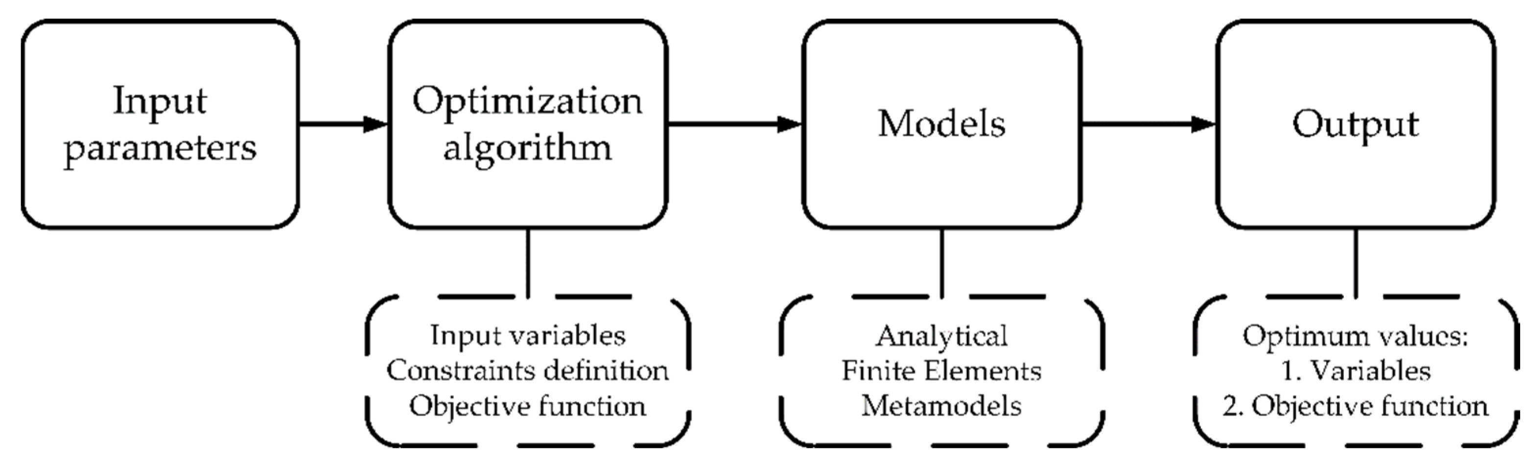
4. Optimization of the PMSM

The search for a better solution in terms of efficiency, mass and cost is a major challenge for the success of electrical machine design. The best way to achieve this goal is to compare different machine topologies that have been optimized to meet the application requirements [9]. In this case, the formulation of an optimization problem consists of using the specifications as constraints to be satisfied and taking the main geometric dimensions and the supply current as optimization variables. The objective functions to be minimized are the mass, the losses and the cost.

During the iterative process, the optimization algorithm uses the performance’s evaluation of the electric motor which corresponds to the values of the variables it has generated. These results are used to propose a new set of dimensions that minimizes the deviations with the constraints to be reached, while improving performance [8]. Two large families of optimization methods can be found: gradient-based algorithms and intelligent algorithms. The first family includes the conjugate gradient algorithm and the sequential quadratic programming algorithm, while the second family includes evolutionary algorithms such as genetic algorithms and multi-objective optimization algorithms [15].

Figure 3 shows in a general way the scheme for solving an optimization problem. Known parameters serve as input to the problem that will be formulated through input variables to be optimized, respecting the constraints and minimizing (or maximizing) an objective function, using an optimization algorithm. The optimization is carried out on a model that will allow verification of compliance with the imposed restrictions. Finally, the output will be the optimal value of the input variables of the objective function.

We also distinguish the different CAD procedures of electrical machines with optimization according to the models used or the ability to explore a domain of solutions with fast models. This is particularly the case of a method that only uses finite element models that we call FEA direct optimization [15]. This is also the case of the space mapping method which allows significant reduction in computational effort and execution time [23,24,25]. This method is well adapted when there is a considerable amount of design candidates. These two approaches will be discussed below.

4.1. Direct FEA Optimization

With this approach, the structure is optimized directly using finite element models to assess the goals and constraints of the optimization problem. An iterative algorithm improves the geometry. These multiphysic models can be in 2D or 3D and can be dynamic or static. They have excellent accuracy in the results, but they are computationally expensive, so some compromises have to be made to minimize computation times [15].

A solution to reduce the size of the problem to be solved is to minimize the number of meshes. This compromises the precision, but running each iteration is faster. The sensitivity during the optimization process will be higher than in analytical models because there are few simplifying assumptions. The result of this optimization with a coarse mesh can serve as a first solution to the optimization process of the structure, and can be repeated with a denser mesh [18].

4.2. Space Mapping Optimization

The SM technique is based on optimization using surrogate models by calibrating coarse models to align them with computationally intensive fine models. Fine models are often FEA, and coarse models are analytical [23]. The coarse model is enhanced by using sample points from a fine model, strategically assigned. Consequently, it represents an approximation to the fine model with a faster response time. It should describe the typical variations of the main physical output quantities as a function of the input design variables [17]. Using SM, it is possible to modify the coarse model with correction factors to minimize discrepancies between the coarse and fine model responses. In this sense, SM combines a computationally cheaper model with a correction based on a more expensive model that helps in the optimization process [15]. The SM optimization process begins with the coarse model, using any optimization method such as generalized reduced gradient (GRG2), to name a few. After performing this optimization, the geometric parameters of the optimal solution are used as inputs to the fine model to perform another more accurate simulation. The results of the fine model simulation are compared to the results of the coarse model. If some differences are observed, then an adjustment of the coarse model must be achieved using correction factors that will allow the coarse model results to align with the fine model results. These correction factors refer to the ratio of the fine model outputs to the coarse model outputs, using the same input parameters. Another optimization must then be performed using the corrected coarse model to find a new optimal point. This process is repeated and the correction factors are updated with each iteration until their value no longer changes and the two models give the same results. Figure 4 shows a flowchart to illustrate this concept developed in [24,25].

Each optimization solution obtained with the coarse model is analyzed with the fine model under the same conditions. If there are differences between the two models, the correction factors are adjusted to repeat an optimization with the coarse model. This process is repeated until the fine model validates the performance of the optimization solution.

Mathematically the computationally cheaper and coarse model can be denoted by $c\left(z\right)\in {\Re }^m$ with $z \in Z \subset {\Re }^n$ and the computationally expensive and fine model is denoted by $f\left(x\right) \in {\Re }^m$. The nonlinear constraints of the coarse and fine models are $r_c\left(x\right)$ and $r_f\left(x\right)$, respectively. In this way, the optimization problem can be expressed as shown in (2):

$$x^{*}=\underset{x\in X}{\arg \min \Vert }f\left(x\right)-y\Vert subject to r_f\left(x\right)\le 0$$

(2)

where $y \in {\Re }^m$ denotes the vector of design specifications. The optimization problem consists of finding a vector $x$ of $n$ input variables that minimizes the distance between the responses of the fine model $f\left(x\right)$ and the desired specifications defined in the vector $y$, then, $x^{*}$ denotes the optimal input values. This problem is hard to solve because it takes a long time to find the optimal solution. To solve this drawback, the optimization is performed with the approximate model $c\left(x\right)$, replacing the fine model $f\left(x\right)$ with the coarse model, and then the problem is replaced by a solution in SM denoted by (3).

$$x^{*}=\underset{x\in X}{\arg \min \Vert }{K}_i\left(c\left(x\right)\right)-y\Vert subject to R_i\left(r_c\left(x\right)\right)\le 0$$

(3)

where $K_i$ and $R_i$ are the correction factors for the objective and constraint functions, respectively. To compute the correction factors, a reasonableness coefficient $\left({\alpha }_r\right)$ with $0<{\alpha }_r<1$ is defined. The correction factors are initialized to 1 for the first optimization of the analytical model, using SM. As indicated in Figure 4, an optimization is carried out with the fine model and the value of the correction factor for the parameter $v$ is updated using Equation (4) [26].

$$K_v=\left(1-{\alpha }_r\right)K_{vi-1}+{\alpha }_r{K}_{vi}$$

(4)

Equation (5) shows how the correction factors are updated.

$$K_{vi}=\frac{v_{FE}}{v_{AM}}$$

(5)

where $v_{FE}$ and $v_{AM}$ represent value of the parameter $v$ by finite elements and analytical models, respectively. Equations (4) and (5) exemplify obtaining a single correction factor, but it is possible to repeat the correction process for the other parameters. The factor(s) given in (4) modify the results of the coarse model to be used in the optimization process as shown in (3) and are updated according to (5) after comparing the output results of the two models. This process is repeated until the coarse model is sufficiently aligned with the fine model such that the difference (error) between the outputs of the two is less than an established tolerance.

To solve the problem using SM, it is possible to use different techniques reported in the literature, including among them Output Space Mapping (OSM), Manifold Mapping (MM) and Kriging-OSM [27]. The first one is the easiest to implement compared to the others because it avoids the process of extracting parameters. MM is an improvement of OSM and allows for the finding of a solution to those where the OSM does not find a correct optimal solution. Finally, Kriging-OSM makes it possible to provide a sufficiently accurate modified coarse model through adaptive corrective mapping [27].

5. Design Example

This section shows an example of a PMSM design problem for an aircraft application [6]. The main challenge is to maximize motor power density and efficiency. We have chosen to set a target for the losses in the motor, which amounts to fixing the efficiency and minimizing the mass. Direct FEA and SM are the two optimization methods that are compared in this example. This involves checking the convergence of each method, analyzing the differences between the solutions and quantifying the computation times.

Design specifications are shown in

Table 2. Design specifications of the machine to be analyzed.

Specification	Name	Units	Value
Nominal Mechanical power	$P_{meca}$	W	160,000
Nominal Rotation speed	$N_{rpm}$	RPM	15,000
Shaft torque	$T_{arbmot}$	Nm	101.9

and

Table 3. Input constant parameters.

Specification	Name	Units	Value
Input parameters
Stator Phase number	$m_{ph}$	-	3
Number of turns per coil	$N_{sp}$	-	1
Winding factor	$k_w$	-	0.933
Number of slots per pole and per phase	$S_{pp}$	-	2
Number of winding layers	$N_{couch}$	-	2
Rotor sleeve thickness	$e_{fret}$	m	0.0005
Mechanical air gap thickness	$e_{var}$	m	0.001
Stator teeth maximal induction	$B_{satd}$	T	1.7
Stator yoke maximal induction	$B_{satc}$	T	1.7
Remanent magnetization of magnet at 100 °C	$B_r$	T	1.136
Stator slot fill factor	$\alpha$	-	0.4
Teeth tips thickness or slot wedge thickness	$e_{cbec}$	m	0.003
Material mass density
Copper	$r{o}_{cu}$	kg/m3	8933
Iron (sheet)	$r{o}_{fer}$	kg/m3	7872
Carbon Sleeve	$r{o}_s$	kg/m3	1500
Magnet	$r{o}_{aim}$	kg/m3	8300
Magnetic material parameters
Electrical conductivity of electrical steel (120 °C)	$\sigma$	S/m	2,083,333
Stator electrical sheet thickness	$d$	m	0.000163
Sheet steel mass density	$r{o}_{tol}$	kg/m3	7650
Fill coefficient	$k_{fois}$	-	1
Hysteresis coefficient	$x_{hys}$	-	223
Excess loss coefficient	$x_{exce}$	-	0.524

, which also show the input constant parameters of the selected radial airgap motor structure with an inner rotor.

6. Optimization Problem Definition

6.1. Space Mapping Optimization

The optimization problem is defined with seven input variables and the objective function to minimize is the mass of motor active parts.

Table 4. Optimization variables for SM.

Parameter Description	Name	Units	Constraint
Magnet thickness	$l_a$	m	0.001 $\le l_a\le$ 0.01
Magnetic circuit axial length	$L$	m	0.02 $\le L\le$ 0.5
Stator inner diameter	$D$	m	0.03 $\le D\le$ 0.5
Stator rms current density	$J$	A/m2	1 × 106 $\le J\le$ 4 × 107
Teeth concentration factor	$k_{teeth}$	-	1.1 $\le k_{teeth}\le$ 10
Yoke concentration factor	$k_{yoke}$	-	0.3 $\le k_{yoke}\le$ 10
Total copper area in stator slots	$S_{cu}$	m2	0.00001 $\le S_{cu}\le$ 0.02

shows the optimization variables with their restriction range.

Table 5. Optimization constraints for SM.

Parameter Description	Units	Constraint
Motor Form factor	-	$Formf\le$ 5
Cooling effort	W/(m3Ohm)	$A{J}_{eq}\le$ 2 × 1012
Peripheral speed	m/s	$v_{peri}\le$ 150
Yoke flux density	T	$B_c\le B_{satc}$
Teeth flux density	T	$B_d\le B_{satd}$
Teeth Form factor	-	$Formft\le$ 5
Total losses	W	$P_{tot}\le$ 3000
Shaft torque	Nm	$T_{arbmot}\ge$ 101.86

completes the constraints that are imposed on the problem.

Five correction factors are considered to improve accuracy of the analytical models during the SM optimization problem, as shown in

Table 6. Correction factors (CF).

Parameter Description	Name	Units	Equation Modified by CF
CF inductance	$k_{Lcs}$	-	$L_{cs}=k_{Lcs}\left(\frac{3{\left(N_{sp}\right)}^2{L}_o}{2}\right)$
CF teeth flux density	$k_{Bd}$	-	$B_d=k_{Bd}\left(\frac{B_{moy}}{1-k_e}\right)$
CF magnetic stator losses	$k_{fer}$	-	$P_{fer}=k_{fer}\left(P_{fery}+P_{fert}\right)$
CF electromagnetic torque	$k_{coupl}$	-	$T_{em}=k_{coupl}\left(\frac{K_{w}LD{B}_{f}J{S}_{cu}}{2\sqrt{2}}\right)$
CF yoke flux density	$k_{Bc}$	-	$B_c=k_{Bc}\left(\frac{B_{moy}{k}_{yoke}}{2}\right)$

.

The method used to find optimal solutions from the analytical models is a nonlinear resolution method based on the generalized reduced gradient (GRG2). A multistart method for global optimization allows exploring the solution domain and is well suited for Space Mapping. Several random starting points are automatically tested with the GRG method to identify the best of the local optimal solutions. The analytical models used during the optimization process are enhanced using OSM. For each optimization solution, the result is analyzed with a fine model simulation (FEA) to adjust the correction factors and restart another optimization with the coarse models. The error must gradually decrease until a final fully validated optimal solution is found.

Figure 5 shows the execution diagram of the space mapping technique including the model correction method with FE.

The time used $\left(t_{tot-SM}\right)$ to carry out the optimization process is counted as shown in (6)

$$t_{tot-SM}={\displaystyle \sum }_{i=0}^n\left(t_{ai}+t_{bi}\right)$$

(6)

For the i-th iteration, $t_{ai}$ is the simulation time of the optimization process with the coarse model, $t_{bi}$ is the simulation time by FE for the validation of optimal solutions and n represents the number of iterations executed until reaching a final valid result. For the FE validation, three magneto dynamic simulations are carried out: the first is a no-load test, the second calculates the cyclic inductance and the third is the nominal load condition. 1.5 electrical periods will be considered in order to compute the iron losses using the Bertotti model.

6.2. Direct FEA Optimization

For the Direct FEA Method, the same motor geometry is optimized with the Matlab function “fmincon” with the “sqp” algorithm. The function handles given in parameters of “fmincon” starts the finite element software using python scripts which construct and simulate the motor performance. Optimization variables and output of the constraint functions are scaled from 0 to 1. Figure 6 shows the detail of the geometry of the machine to be optimized. The optimization problem is defined with eight input variables and

Table 7. Optimization variables for Direct FEA.

Parameter Description	Name	Units	Constraint
Slot depth	$H_{es}$	m	0.01 $\le H_{es}\le$ 0.014
Rotor inner diameter	$D_{int}$	m	0.07 $\le D_{int}\le$ 0.105
Magnet thickness	$l_a$	m	0.005 $\le l_a\le$ 0.01
Slot opening angle	${\theta }_e$	Rad	0.065 $\le {\theta }_e\le$ 0.090
Stator yoke thickness	$e_{culs}$	m	0.005 $\le e_{culs}\le$ 0.008
Magnetic circuit axial length	$L$	m	0.14 $\le L\le$ 0.185
Nominal RMS phase current	$I_s$	A	170 $\le I_s\le$ 250
Current control angle	$P_{si}$	Deg	−15 $\le P_{si}\le$ −5

details their constraints range.

Table 8. Optimization constraints for Direct FEA.

Parameter Description	Units	Constraint
Electromagnetic torque	Nm	$T_{em}\ge$ 103.5
Total losses	W	$P_{tot}\le$ 3000
Cooling effort	W/(m3Ohm)	$A{J}_{eq}\le$ 2 × 1012
Yoke flux density	T	$B_c\le B_{satc}$
Teeth flux density	T	$B_d\le B_{satd}$

completes the restrictions imposed in this optimization problem.

By comparing Table 4 and Table 7, we can notice that several variables are different with respect to the problem solved with the analytical model in the SM process. This is due to the form of the analytical model which uses different input variables. In the case of the finite element model, these are the geometric dimensions and the power supply used with the current amplitude and the control angle.

7. Results

7.1. Space Mapping

The objective function proposed in the problem is the minimization of the total weight of the active parts of the motor. Figure 7 shows the evolution of the optimization results for each iteration of the analytical model correction process with FEA.

It can be seen that the results converge in seven iterations and that the final mass of the active parts corresponds to 14.7 kg and the power density estimated with the active parts weight is 10.9 kW/kg.

Figure 8 shows the distribution of the losses of the machine, namely the losses due to the Joule effect, to the iron of the stator and to the additional losses (aerodynamic losses). It can be seen that the convergence is very fast. The total losses of the machine remain constant after the second iteration at 3 kW. Joule Losses represent approximately 2/3 of the total losses of the machine.

Figure 9 shows the magnetic induction in different parts of the machine structure such as the yoke, the stator teeth and the airgap. The magnetic induction in the yoke and in the teeth reach the constraint value in the third iteration. These quantities must be limited to avoid magnetic saturation in the machine since the analytical model assumes that magnetic materials have linear characteristics. Nonlinear characteristics are only taken into account in the finite element model which is used for the correction method.

As indicated in previous sections, in the SM technique it is necessary to use correction factors to reduce the discrepancies between the coarse and the fine model. Figure 10 shows the evolution of the correction factors during the optimization process. The correction factors of the torque and the inductance show the greatest variations. These variations arise after each iteration, when the coarse model is adjusted to get as close as possible to the results produced by the fine model. After the seven iterations, the error with the fine model is negligible, which confirms that optimal solution found with the analytical model is valid. The final value of each correction factor shows the error of the uncorrected analytical model for the five parameters considered.

Figure 11 shows the result of the electromagnetic torque of the optimal solution after each iteration with the fine model for the correction of the coarse model. The final value of electromagnetic torque is 102.83 Nm as expected with the specification.

Figure 12 shows the evolution of geometry for each iteration until the valid optimal solution is found. It is observed that geometric parameters such as magnet outer diameter, stator outer diameter, rotor inner diameter, slot depth, among others, vary significantly between each iteration.

Table 9. Optimal results obtained by SM and validation.

Parameter Description	Units	Optimal Value
Magnet thickness	m	0.010
Motor axial length	m	0.167
Stator inner diameter	m	0.112
Stator rms current density	A/m2	1.50 × 107
Teeth concentration factor	-	2.984
Yoke concentration factor	-	3.661
Total copper area in stator slots	m2	0.0014
Calculated parameters
Parameter Description	Units	FEA validation	SM	Error (%)
Electromagnetic Torque	Nm	102.54	102.83	−0.28
Total active parts weight	kg	14.79	14.68	0.74
Total losses	W	2990	3000	−0.33
Fundamental magnetic induction	T	0.933	0.946	−1.39
Teeth flux density	T	1.72	1.7	1.16
Yoke flux density	T	1.71	1.7	1.16
Nominal phase current	Arms	218.90	218.90	0
Electrical phase resistance	Ohm	0.0134	0.0137	−2.24
Cooling effort	W/(m3Ohm)	8.46 × 1011	8.48 × 1011	−0.24
Magnetic stator losses	W	941	933	0.85

shows the optimal results obtained by SM and the percentage of errors found between the coarse model and the fine model (reference) at the end of the validation process.

For each iteration, the time required for optimization with the coarse model was $t_{ai}$ = 1 min and the time required to validate the results using the FE technique was $t_{bi}$ = 9 min. In this way, the total simulation time $\left(t_{tot-SM}\right)$ for the space mapping technique is

$$t_{tot-SM}={\displaystyle \sum }_{i=0}^{7}1+9=80 \min$$

Finally, Figure 13 shows a comparison of the magnetic induction in the air gap of the machine, determined with the analytical expression reported in [21] and by means of the FEM. This confirms the analytical model provides a good estimation of the flux density in the air gap knowing that this model is not corrected.

7.2. FEA

Figure 14 shows the mesh density of the motor geometry which is optimized with finite elements. This mesh has 5724 nodes and a complete analysis of a structure required three transient simulations which take into account the rotation with 30 rotor positions per 1.5 electrical period. This gives a time of 150 s (≈0.0417 h) to complete the scan of a machine. A total of 129 machines were considered and the optimization required 10 major iterations, which corresponds to a total of 5.38 h for a personal computer (16 GB of RAM with an i7 processor). It should be noted that the initial structure for this optimization corresponds to that found with the SM method.

Table 10. Optimal results for FEA.

Parameter Description	Units	Optimal Value
Slot depth	m	0.014
Rotor inner diameter	m	0.098
Nominal RMS phase current	A	242
Slot opening angle	rad	0.084
Stator yoke thickness	m	0.0059
Motor axial length	m	0.15
Machine control angle	deg	−10.97
Magnet thickness	m	0.007

shows the values of the optimized variables and

Table 11. Performance of the machine for the optimal design found.

Parameter Description	Units	Value
Electromagnetic Torque	Nm	103.5
Total active parts weight	kg	14.25
Total losses	W	3000
Fundamental magnetic induction	T	0.83
Teeth flux density	T	1.7
Yoke flux density	T	1.58
Nominal phase current	Arms	242
Electrical phase resistance	Ohm	0.011
Cooling effort	A2/m3	9.20 × 1011

gives the results of the performance of this machine.

8. Discussion

Starting from different optimization variables and constraints, a motor PM with Halbach array was optimally designed using two different techniques: Space mapping and Direct FEA. Space mapping was applied to the analytical machine sizing model and its outputs were fitted with a small number of FE simulations to find some correction factors. Only seven simulations were necessary to converge towards a valid optimal solution. The correction factor of the electromagnetic torque $\left(k_{coupl}\right)$ indicates that the analytical model underestimates the torque by 16%. Therefore, the same optimization without correction of the analytical model is not acceptable and leads to results that are not valid.

Table 12. Comparison of the optimal results found by the space mapping and optimization direct techniques.

Parameter Description	Units	FEA	SM	Difference (%)
Electromagnetic Torque	Nm	103.5	102.8	+0.7
Total active parts weight	kg	14.25	14.68	−3
Total losses	W	3000	3000	0.0
Fundamental magnetic induction	T	0.83	0.946	−14
Teeth flux density	T	1.58	1.7	−7.6
Yoke flux density	T	1.7	1.7	0.00
Nominal phase current	Arms	242	218.90	+9.6
Electrical phase resistance	Ohm	0.0110	0.0137	−24.6
Magnetic stator losses	W	888	933	−5.1
Power density	kW/kg	11.41	10.90	+4.5
Simulation time	h	5.38	1.2	+77.7

summarizes the comparison of the optimal results found by the SM technique and direct FEA. In the SM technique, the convergence towards an optimal solution is made according to the sensitivity of the coarse model. The correction mechanism implemented only corrects the accuracy of the coarse model. Therefore, the optimal solution is valid with good accuracy but obtaining the best optimum of the problem is not guaranteed.

The solution found by means of the SM technique met the torque specifications with a margin of error of less than 1%. However, we showed that the optimization of this geometry is not the optimal solution of the problem since it has been improved with the direct FE optimization method. The sensitivity of the fine model is therefore greater than that of the analytical model. Nevertheless, the gain on the total mass is only 430 g, which represents a reduction of 3%. Even if the length of the motor has been reduced by 10%, it can be seen that the impact on the total mass of the motor is not significant because the diameter has increased slightly. This geometric modification is also reflected by a reduction in the no-load flux per phase, an increase in the current and an increase in the section of conductors.

However, the total simulation time is significantly reduced with the SM. Indeed, it requires less than 20% of the computation time compared to direct FE optimization. This is an essential advantage to better explore the whole field of study with a multistart method. The running time of 5.38 h is relatively low for the FE simulation because the mesh density is low and the starting point of this optimization is based on the results obtained by the SM. This accelerated the convergence towards the final solution and reduced the number of iterations or machines studied. With another starting point, the average resolution time should be around 9 h [15].

In this work, an analytical model was used as a coarse model, unlike what was reported in [14], which involved the use of a less dense FE model. Similarly, the approach considered in this work allows a reduction in computational time by a factor greater than 4.5, unlike the authors of [14] who report a factor of 2.5. It was also demonstrated that the sensitivity of the analytical model is very good and ensures convergence towards a solution close to the optimum.

9. Conclusions

In this work, a comparison was made between Space Mapping and direct FEA optimization to find an optimal geometry of a PM motor with Halbach array. The results show that the Space Mapping method converges easily, in a few iterations, with a correction of the model by FEA. It was possible to obtain a valid optimal solution with a nonlinear resolution method based on the generalized reduced gradient (GRG2) and a multistart option. The SM method has already been successfully applied for the design of high-performance machines and the exploration of a wide array of solutions. However, there was no real comparison between the solution found by SM and the solution of a direct optimization by the fine elements model. We know that changing the model accuracy leads to a modification of the final solution in an optimization process and we see an improvement if the optimization is done directly with the finite element model. This article allows for the quantification of the differences between the two optimization methods for the specifications of a PM motor for an aircraft application.

A considerable advantage was found in the computational cost of this method compared to a direct optimization by FEA. This saves simulation time and allows a large amount of designs to be studied to explore the whole solutions domain in more detail.

Similarly, the comparison between the solution found by the Spatial Mapping optimization method with that obtained by the direct FEA optimization method shows that these solutions are very close (the difference in mass of the active parts is only 3%). Even if the geometry has been slightly modified, it is obvious that the FEA optimization does not significantly improve the results obtained by Space Mapping.

The correction of the electrical model including the value of the inductance makes the analytical model sufficiently efficient to take into account a constraint on the supply voltage. The analytical model can also be easily improved to estimate the additional losses in the magnets without affecting the performance of the optimization by Space Mapping.

In summary, this study demonstrates that the Space Mapping Method is a very powerful method to optimize the power density of electric motors:

-

There is an important reduction in computing time with SM. Almost an 80% time reduction was found, considering that for direct FEA optimization, the mesh density is low and the starting point of this optimization was based on the results obtained by the SM method.

-

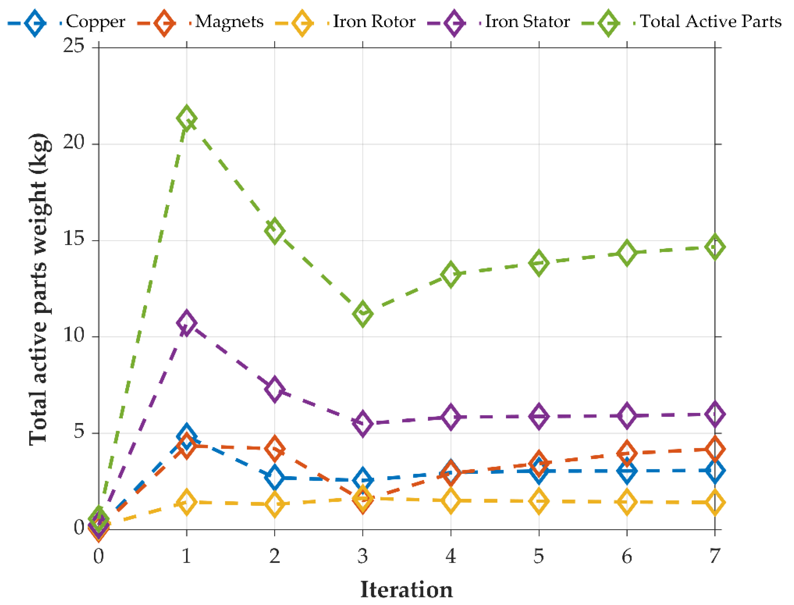
The motor geometry of the final solutions of both optimization methods is different but the motor mass difference is small (less than 3%). Power density and torque density are very similar.

References

1. Zhang, R.; Fujimori, S. The role of transport electrification in global climate change mitigation scenarios. Env. Res. Lett. 2020, 15, 034019. [Google Scholar] [CrossRef]
2. Varyukhin, A.N.; Zakharchenko, V.S.; Vlasov, A.V.; Gordin, M.V.; Ovdienko, M.A. Roadmap for the Technological Development of Hybrid Electric and Full-Electric Propulsion Systems of Aircrafts. In Proceedings of the—ICOECS 2019: 2019 International Conference on Electrotechnical Complexes and Systems, Ufa, Russia, 21–25 October 2019; IEEE: Piscataway, NJ, USA, 2019. [Google Scholar]
3. Chowdhury, S.; Gurpinar, E.; Su, G.J.; Raminosoa, T.; Burress, T.A.; Ozpineci, B. Enabling Technologies for Compact Integrated Electric Drives for Automotive Traction Applications. In Proceedings of the ITEC 2019—2019 IEEE Transportation Electrification Conference and Expo, Detroit, MI, USA, 19–21 June 2019. [Google Scholar]
4. Ghandriz, T.; Jacobson, B.; Islam, M.; Hellgren, J.; Laine, L. Transportation-mission-based optimization of heterogeneous heavy-vehicle fleet including electrified propulsion. Energies 2021, 14, 3221. [Google Scholar] [CrossRef]
5. Pettes-Duler, M.; Roboam, X.; Sareni, B.; Lefevre, Y.; Llibre, J.F.; Fénot, M. Multidisciplinary design optimization of the actuation system of a hybrid electric aircraft powertrain. Electronics 2021, 10, 1297. [Google Scholar] [CrossRef]
6. Quillet, D.; Boulanger, V.; Rancourt, D.; Freer, R.; Bertrand, P. Parallel Hybrid-Electric Powertrain Sizing on Regional Turboprop Aircraft with Consideration for Certification Performance Requirements. In Proceedings of the AIAA AVIATION 2021 FORUM, Virtual, 2–6 August 2021. [Google Scholar] [CrossRef]
7. Pyrhönen, J.; Jokinen, T.; Hrabovcová, V. Design of Rotating Electrical Machines; John Wiley & Sons: Hoboken, NJ, USA, 2008; ISBN 9780470695166. [Google Scholar]
8. Lei, G.; Zhu, J.; Guo, Y.; Liu, C.; Ma, B. A review of design optimization methods for electrical machines. Energies 2017, 10, 1962. [Google Scholar] [CrossRef] [Green Version]
9. Bramerdorfer, G.; Tapia, J.A.; Pyrhönen, J.J.; Cavagnino, A. Modern Electrical Machine Design Optimization: Techniques, Trends, and Best Practices. IEEE Trans. Ind. Electron. 2018, 65, 7672–7684. [Google Scholar] [CrossRef]
10. Abdalmagid, M.; Sayed, E.; Bakr, M.H.; Emadi, A. Geometry and Topology Optimization of Switched Reluctance Machines: A Review. IEEE Access 2022, 10, 5141–5170. [Google Scholar] [CrossRef]
11. Vaschetto, S.; Tenconi, A.; Bramerdorfer, G. Sizing procedure of surface mounted PM Machines for fast analytical evaluations. In Proceedings of the 2017 IEEE International Electric Machines and Drives Conference (IEMDC), Miami, FL, USA, 21–24 May 2017; pp. 1–8. [Google Scholar]
12. Xie, P.; Ramanathan, R.; Vakil, G.; Gerada, C. Simplified analytical machine sizing for surface mounted permanent magnet machines. In Proceedings of the 2019 IEEE International Electric Machines and Drives Conference, IEMDC 2019, San Diego, CA, USA, 12–15 May 2019; pp. 751–757. [Google Scholar]
13. Moreno, Y.; Almandoz, G.; Egea, A.; Madina, P.; Escalada, A.J. Multi-physics tool for electrical machine sizing. Energies 2020, 13, 1651. [Google Scholar] [CrossRef] [Green Version]
14. Vivier, S.; Friedrich, G. Comparison between Single-Model and Multimodel Optimization Methods for Multiphysical Design of Electrical Machines. IEEE Trans. Ind. Appl. 2018, 54, 1379–1389. [Google Scholar] [CrossRef]
15. Grenier, J.M.; Pérez, R.; Picard, M.; Cros, J. Magnetic FEA direct optimization of high-power density, halbach array permanent magnet electric motors. Energies 2021, 14, 5939. [Google Scholar] [CrossRef]
16. Krishnan, R.; Bharadwaj, A.S.; Materu, P.N. Computer-Aided Design Of Electrical Machines For Variable Speed Applications. IEEE Trans. Ind. Electron. 1988, 35, 560–571. [Google Scholar] [CrossRef]
17. Ghorbanian, V.; Salimi, A.; Lowther, D.A. A computer-aided design process for optimizing the size of inverter-fed permanent magnet motors. IEEE Trans. Ind. Electron 2017, 65, 1819–1827. [Google Scholar] [CrossRef]
18. Cros, J.; Viarouge, P.; Kakhki, M.T. Design and optimization of soft magnetic composite machines with finite element methods. IEEE Trans. Magn. 2011, 47, 4384–4390. [Google Scholar] [CrossRef]
19. Tiegna, H.; Amara, Y.; Barakat, G. Overview of analytical models of permanent magnet electrical machines for analysis and design purposes. Math. Comput. Simul. 2013, 90, 162–177. [Google Scholar] [CrossRef]
20. Rosu, M.; Zhou, P.; Lin, D.; Lonol, D.; Popescu, M.; Blaabjerg, F.; Rallabandi, V.; Staton, D. Multiphysics Simulation by Design for Electrical Machines, Power Electronics and Drives; Wiley-IEEE Press: Piscataway, NJ, USA, 2018; ISBN 9781119103448. [Google Scholar]
21. Shi, T.; Qiao, Z.; Xia, C.; Li, H.; Song, Z. Modeling, analyzing, and parameter design of the magnetic field of a segmented Halbach cylinder. IEEE Trans. Magn. 2012, 48, 1890–1898. [Google Scholar] [CrossRef]
22. Touhami, S.; Zeaiter, A.; Fénot, M.; Lefevre, Y.; Llibre, J. Electro-thermal Models and Design Approach for High Specific Power Electric Motor for Hybrid Aircraft. In Proceedings of the Aerospace Europe Conference, Bordeaux, France, 25–28 February 2020. [Google Scholar]
23. Cheng, Q.S.; Bandler, J.W.; Koziel, S. A review of implicit space mapping optimization and modelling techniques. In Proceedings of the 2015 IEEE MTT-S International Conference on Numerical Electromagnetic and Multiphysics Modeling and Optimization, NEMO 2015, Ottawa, ON, Canada, 11–14 August 2015; IEEE: Piscataway, NJ, USA, 2015; pp. 9–11. [Google Scholar]
24. Bandler, J.W.; Cheng, Q.S.; Dakroury, S.A.; Mohamed, A.S.; Bakr, M.H.; Madsen, K.; Søndergaard, J. Space Mapping: The State of The Art. IEEE Trans. Microw. Theory Tech. 2004, 52, 337–361. [Google Scholar] [CrossRef]
25. Bandler, J.W.; Biernacki, R.M.; Chen, S.H.; Grobelny, P.A.; Hemmers, R.H. Space Mapping Technique for Electromagnetic Optimization. IEEE Trans. Microw. Theory Tech. 1994, 42, 2536–2544. [Google Scholar] [CrossRef]
26. Cros, J.; Radaorozandry, L.; Figueroa, J.; Viarouge, P. Influence of the magnetic model accuracy on the optimal design of a car alternator. COMPEL Int. J. Comput. Math. Electr. Electron. Eng. 2008, 27, 196–204. [Google Scholar] [CrossRef]
27. Gong, J.; Gillon, F.; Bracikowski, N. Comparison of three space mapping techniques on electromagnetic design optimization. COMPEL Int. J. Comput. Math. Electr. Electron. Eng. 2018, 37, 565–580. [Google Scholar] [CrossRef]
Figure 1. Flowchart for PMSM design in a CAD environment.
Energies 15 03969 g001
Figure 2. CAD environment with coupling of physical models [18].
Energies 15 03969 g002
Figure 3. Scheme for solving an optimization problem.
Energies 15 03969 g003
Figure 4. Flowchart to illustrate the SM concept.
Energies 15 03969 g004
Figure 5. Space mapping technique execution diagram.
Energies 15 03969 g005
Figure 6. Geometry of the machine having seven magnet segments per pole.
Energies 15 03969 g006
Figure 7. Optimal weight of active parts.
Energies 15 03969 g007
Figure 8. Machine losses.
Energies 15 03969 g008
Figure 9. Magnetic induction.
Energies 15 03969 g009
Figure 10. Evolution of correction factors.
Energies 15 03969 g010
Figure 11. Electromagnetic torque of the machine.
Energies 15 03969 g011
Figure 12. Machine geometries for each iteration.
Energies 15 03969 g012
Figure 13. Magnetic induction in the air gap of the machine.
Energies 15 03969 g013
Figure 14. Mesh of the optimized motor.
Energies 15 03969 g014