Figure 1.
100% NG; MAP = 1.2 bar; n = 3500 rpm. (a) Experimental MFB profile and its derivative interpolated with the best matching Wiebe and Hill functions; (b) Experimental and numeric pressure curves, simulated with the best matching Wiebe and Hill functions.
Figure 1.
100% NG; MAP = 1.2 bar; n = 3500 rpm. (a) Experimental MFB profile and its derivative interpolated with the best matching Wiebe and Hill functions; (b) Experimental and numeric pressure curves, simulated with the best matching Wiebe and Hill functions.
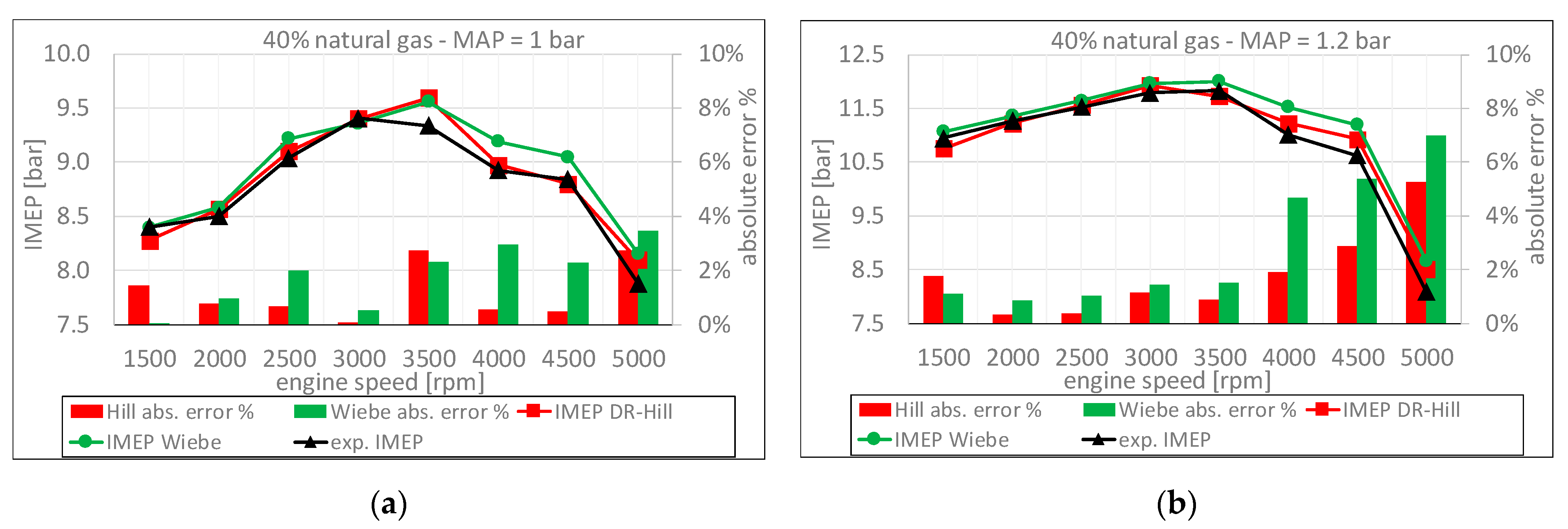
Figure 2.
Comparison between the experimental and simulated IMEP; 40% NG fuel mixture. (a) MAP = 1 bar. (b) MAP = 1.2 bar.
Figure 2.
Comparison between the experimental and simulated IMEP; 40% NG fuel mixture. (a) MAP = 1 bar. (b) MAP = 1.2 bar.
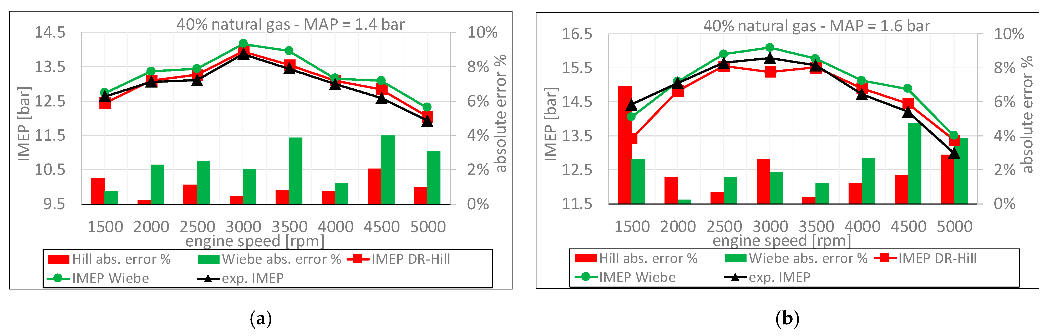
Figure 3.
Comparison between the experimental and simulated IMEP; 40% NG fuel mixture. (a) MAP = 1.4 bar; (b) MAP = 1.6 bar.
Figure 3.
Comparison between the experimental and simulated IMEP; 40% NG fuel mixture. (a) MAP = 1.4 bar; (b) MAP = 1.6 bar.
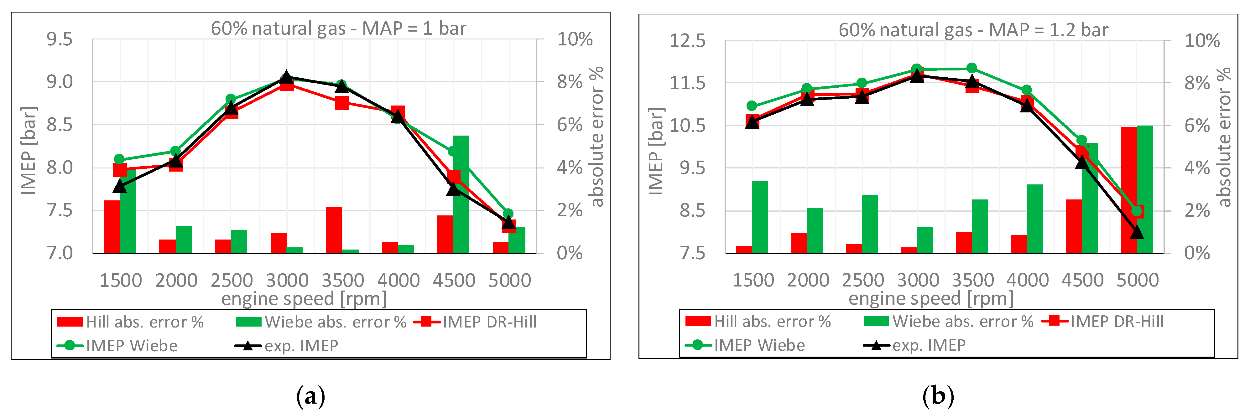
Figure 4.
Comparison between the experimental and simulated IMEP; 60% NG fuel mixture. (a) MAP = 1 bar; (b) MAP = 1.2 bar.
Figure 4.
Comparison between the experimental and simulated IMEP; 60% NG fuel mixture. (a) MAP = 1 bar; (b) MAP = 1.2 bar.
Figure 5.
Comparison between the experimental and simulated IMEP; 60% NG fuel mixture. (a) MAP = 1.4 bar; (b) MAP = 1.6 bar.
Figure 5.
Comparison between the experimental and simulated IMEP; 60% NG fuel mixture. (a) MAP = 1.4 bar; (b) MAP = 1.6 bar.
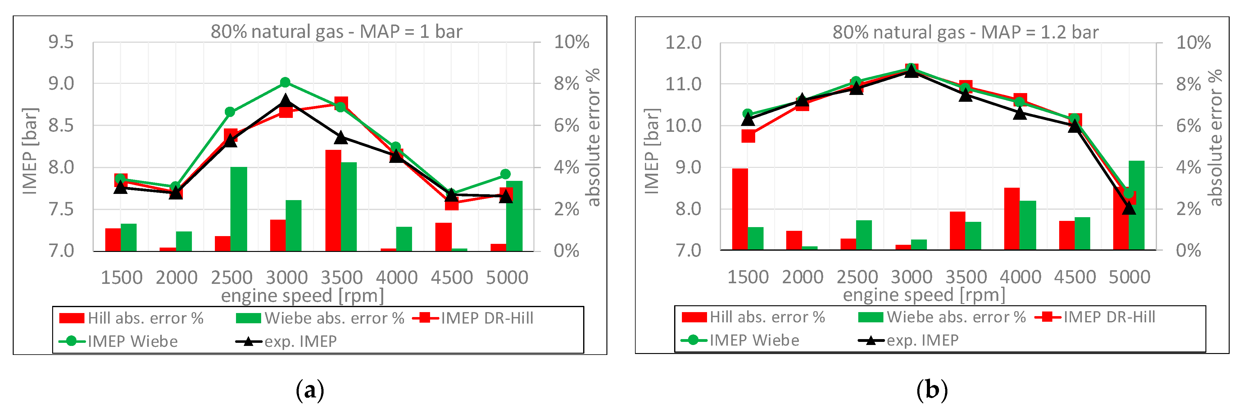
Figure 6.
Comparison between the experimental and simulated IMEP; 80% NG fuel mixture. (a) MAP = 1 bar; (b) MAP = 1.2 bar.
Figure 6.
Comparison between the experimental and simulated IMEP; 80% NG fuel mixture. (a) MAP = 1 bar; (b) MAP = 1.2 bar.
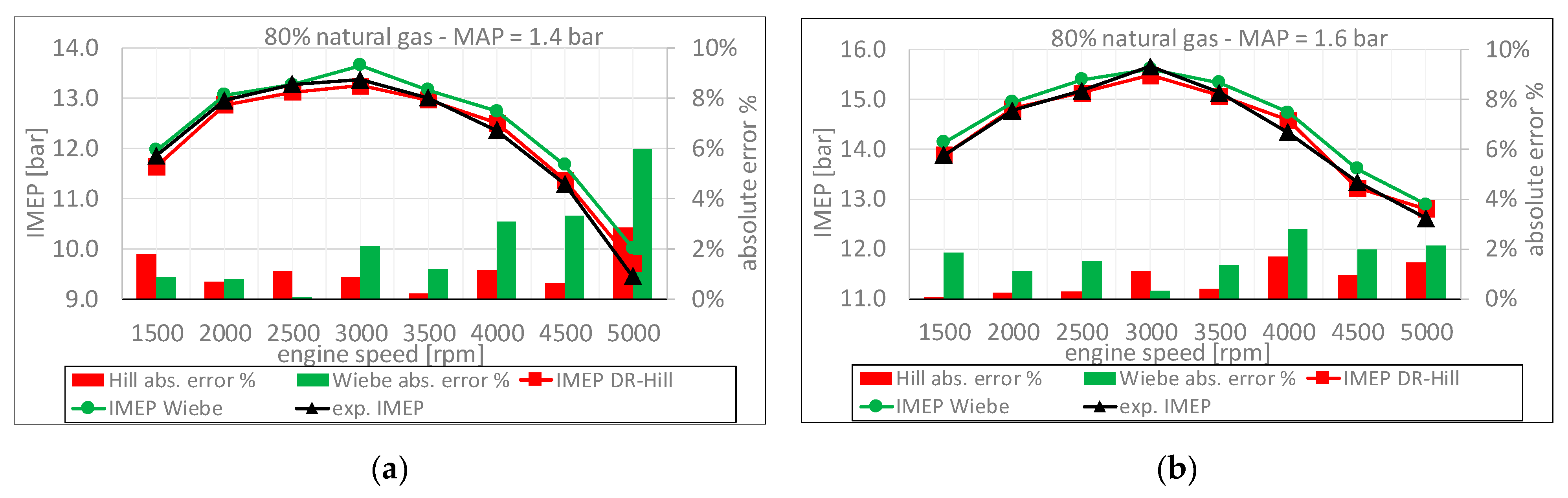
Figure 7.
Comparison between the experimental and simulated IMEP; 80% NG fuel mixture. (a) MAP = 1.4 bar; (b) MAP = 1.6 bar.
Figure 7.
Comparison between the experimental and simulated IMEP; 80% NG fuel mixture. (a) MAP = 1.4 bar; (b) MAP = 1.6 bar.
Figure 8.
MAP = 0.5 bar, engine speed n = 3000 rpm.
Figure 8.
MAP = 0.5 bar, engine speed n = 3000 rpm.
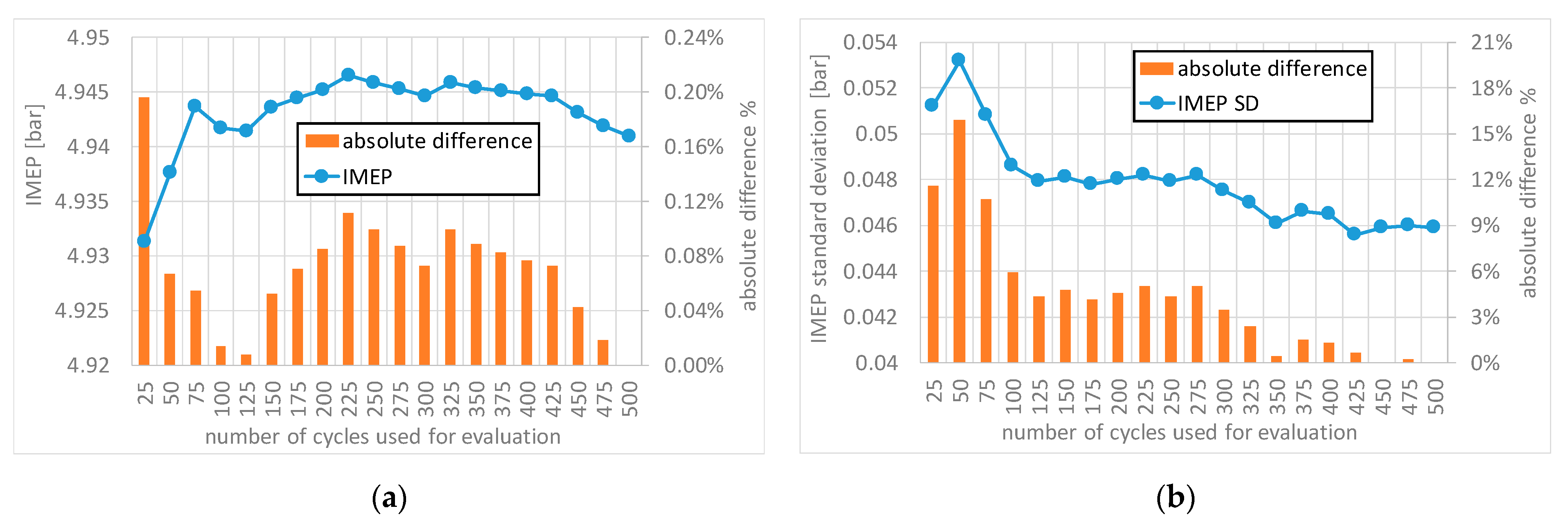
Figure 9.
MAP = 0.5 bar, engine speed n = 3000 rpm. (a) average IMEP and absolute difference% vs. number of cycles taken for evaluation; (b) IMEP SD and absolute difference% vs. number of cycles taken for evaluation.
Figure 9.
MAP = 0.5 bar, engine speed n = 3000 rpm. (a) average IMEP and absolute difference% vs. number of cycles taken for evaluation; (b) IMEP SD and absolute difference% vs. number of cycles taken for evaluation.
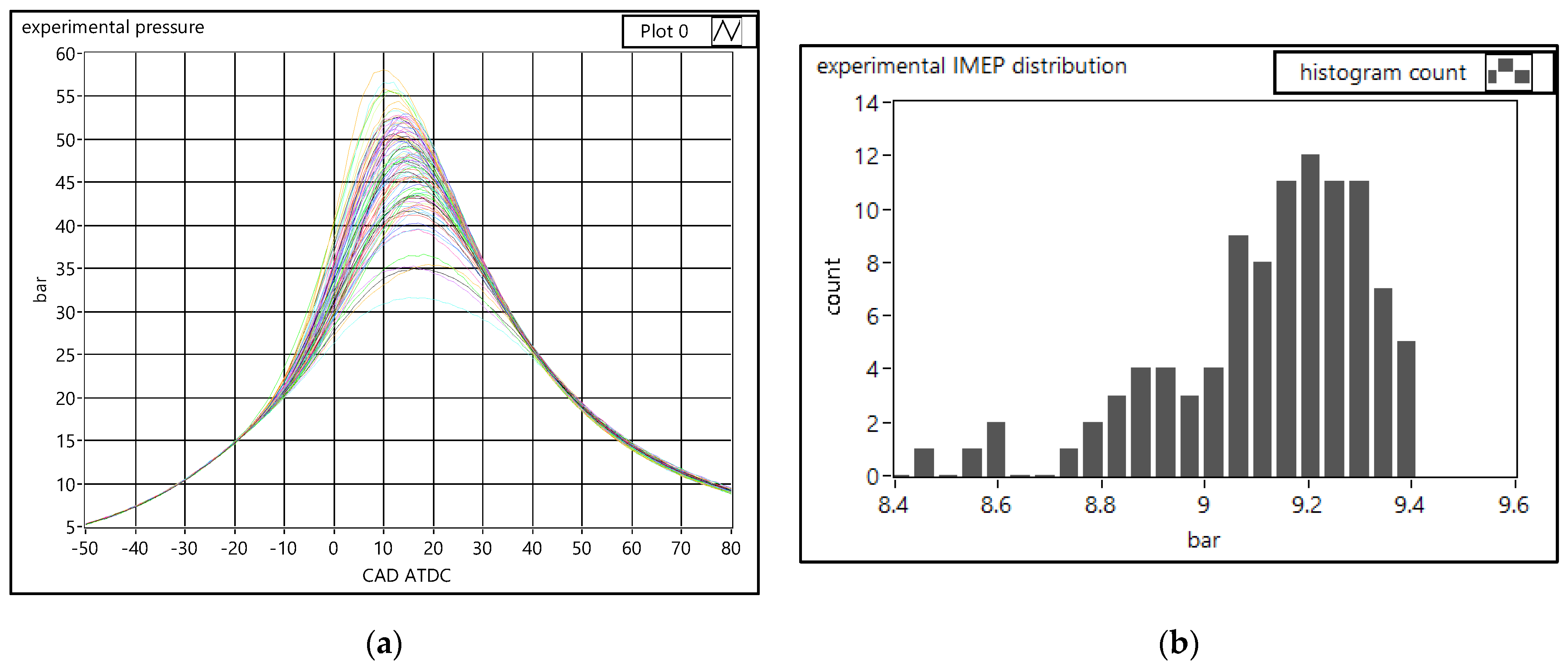
Figure 10.
MAP = 1 bar, engine speed n = 3500 rpm, fuel 100% NG. (a) 100 consecutive pressure cycles; (b) histogram of IMEP distribution (mean value = 9.11 bar, SD = 0.214 bar).
Figure 10.
MAP = 1 bar, engine speed n = 3500 rpm, fuel 100% NG. (a) 100 consecutive pressure cycles; (b) histogram of IMEP distribution (mean value = 9.11 bar, SD = 0.214 bar).
Figure 11.
Histograms of Hill coefficients experimental distribution; MAP = 1 bar, n = 3500 rpm, fuel NG. (a) δ coefficient (mean value = 32.3 CAD, SD = 3.24 CAD; (b) n coefficient (mean value = 4.69, SD = 0.35).
Figure 11.
Histograms of Hill coefficients experimental distribution; MAP = 1 bar, n = 3500 rpm, fuel NG. (a) δ coefficient (mean value = 32.3 CAD, SD = 3.24 CAD; (b) n coefficient (mean value = 4.69, SD = 0.35).
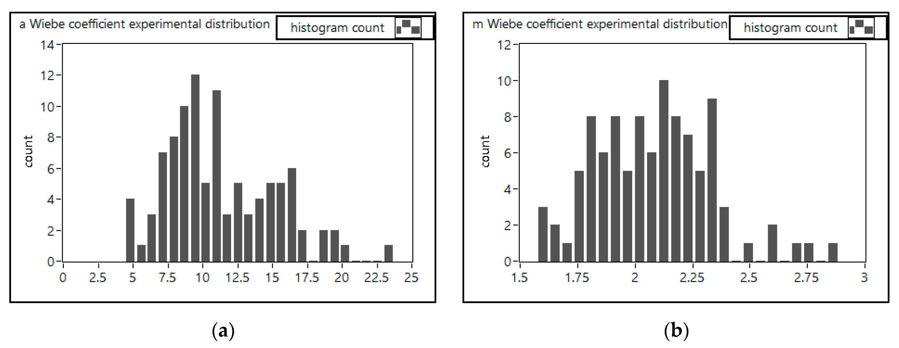
Figure 12.
Histograms of Wiebe coefficients experimental distribution; MAP = 1 bar, n = 3500 rpm, fuel NG. (a) a coefficient (mean value = 11.2, SD = 3.93); (b) m coefficient (mean value = 2.08, SD = 0.254).
Figure 12.
Histograms of Wiebe coefficients experimental distribution; MAP = 1 bar, n = 3500 rpm, fuel NG. (a) a coefficient (mean value = 11.2, SD = 3.93); (b) m coefficient (mean value = 2.08, SD = 0.254).
Figure 13.
Histograms of Hill coefficients numeric distribution; MAP = 1 bar, n = 3500 rpm, fuel NG. (a) δ coefficient (mean value = 32.3 CAD, SD = 3.24 CAD); (b) n coefficient (mean value = 4.69, SD = 0.35).
Figure 13.
Histograms of Hill coefficients numeric distribution; MAP = 1 bar, n = 3500 rpm, fuel NG. (a) δ coefficient (mean value = 32.3 CAD, SD = 3.24 CAD); (b) n coefficient (mean value = 4.69, SD = 0.35).
Figure 14.
Histograms of Wiebe coefficients numeric distribution; MAP = 1 bar, n = 3500 rpm, fuel NG. (a) a coefficient (mean value = 11.2, SD = 3.93); (b) m coefficient (mean value = 2.08, SD = 0.254).
Figure 14.
Histograms of Wiebe coefficients numeric distribution; MAP = 1 bar, n = 3500 rpm, fuel NG. (a) a coefficient (mean value = 11.2, SD = 3.93); (b) m coefficient (mean value = 2.08, SD = 0.254).
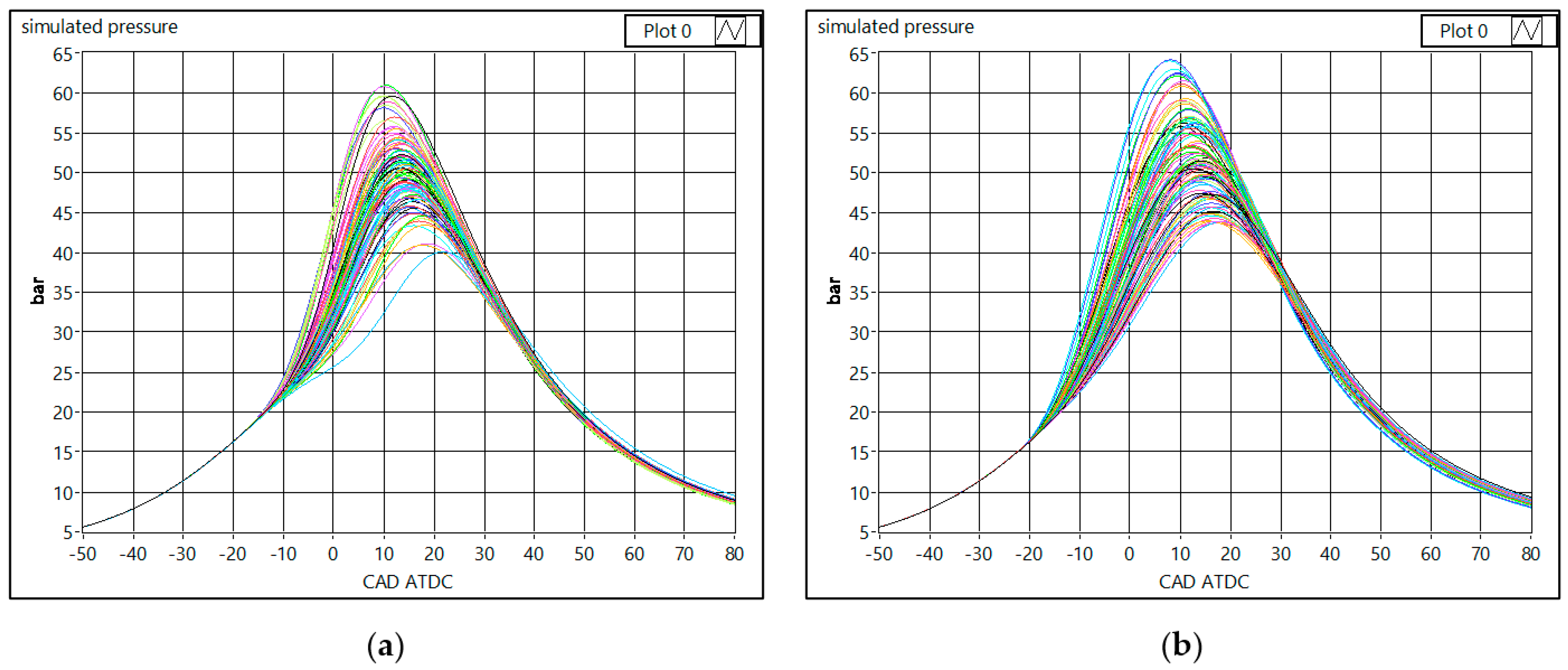
Figure 15.
100 simulated pressure cycles; MAP = 1 bar, engine speed n = 3500 rpm, fuel 100% NG. (a) using the Hill function; (b) using the Wiebe function.
Figure 15.
100 simulated pressure cycles; MAP = 1 bar, engine speed n = 3500 rpm, fuel 100% NG. (a) using the Hill function; (b) using the Wiebe function.
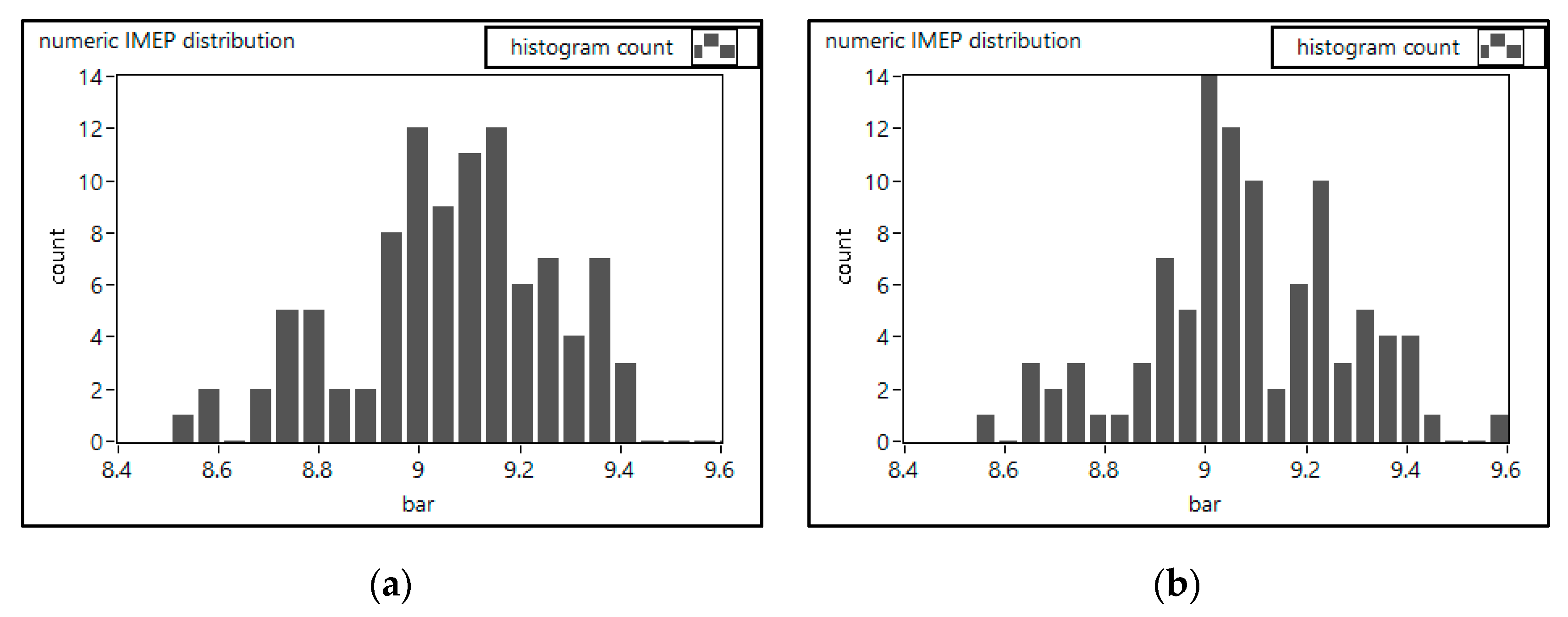
Figure 16.
Histogram of numeric IMEP distribution; MAP = 1 bar, n = 3500 rpm, fuel NG. (a) Hill function, (mean value = 9.07 bar, SD = 0.222 bar); (b) Wiebe function, (mean value = 9.15 bar, SD = 0.206 bar).
Figure 16.
Histogram of numeric IMEP distribution; MAP = 1 bar, n = 3500 rpm, fuel NG. (a) Hill function, (mean value = 9.07 bar, SD = 0.222 bar); (b) Wiebe function, (mean value = 9.15 bar, SD = 0.206 bar).
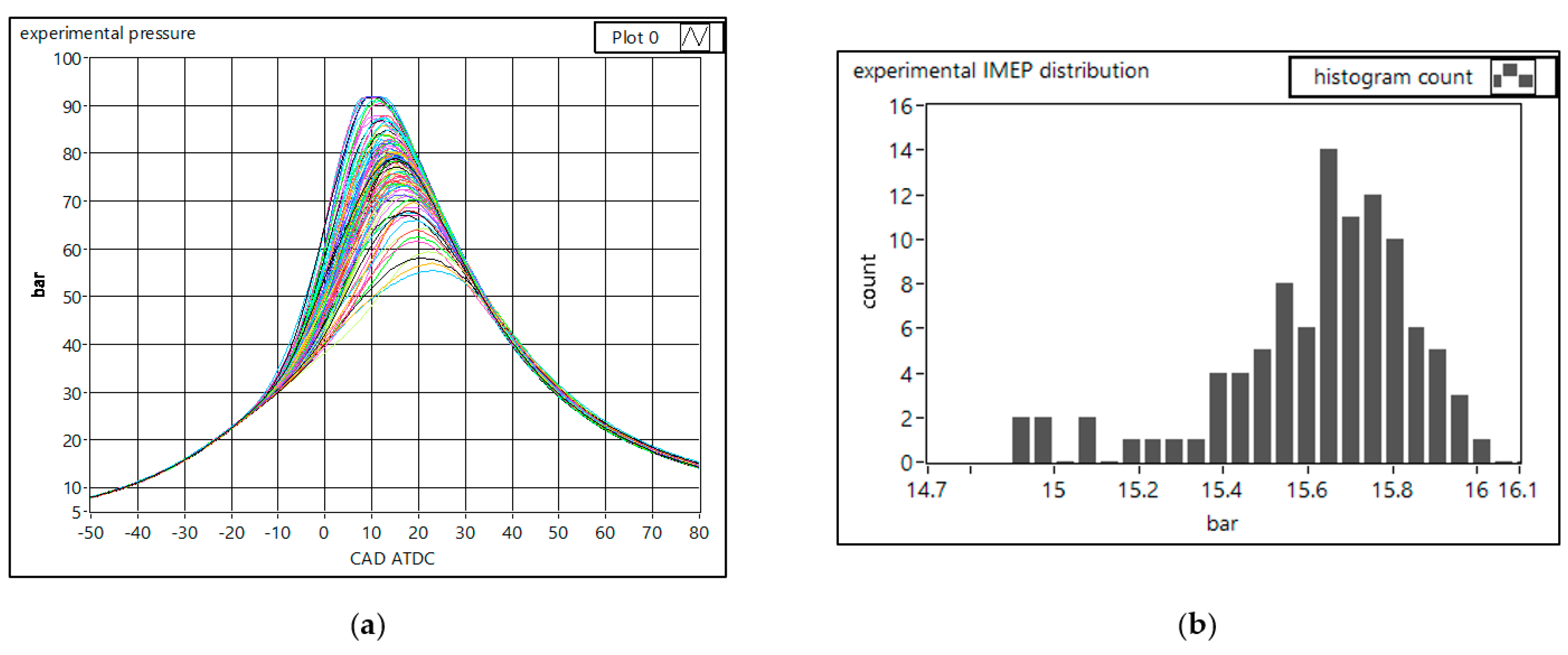
Figure 17.
MAP = 1.6 bar, engine speed n = 2500 rpm, fuel 100% NG. (a) 100 consecutive pressure cycles; (b) histogram of IMEP distribution (mean value = 15.6 bar, SD = 0.239 bar).
Figure 17.
MAP = 1.6 bar, engine speed n = 2500 rpm, fuel 100% NG. (a) 100 consecutive pressure cycles; (b) histogram of IMEP distribution (mean value = 15.6 bar, SD = 0.239 bar).
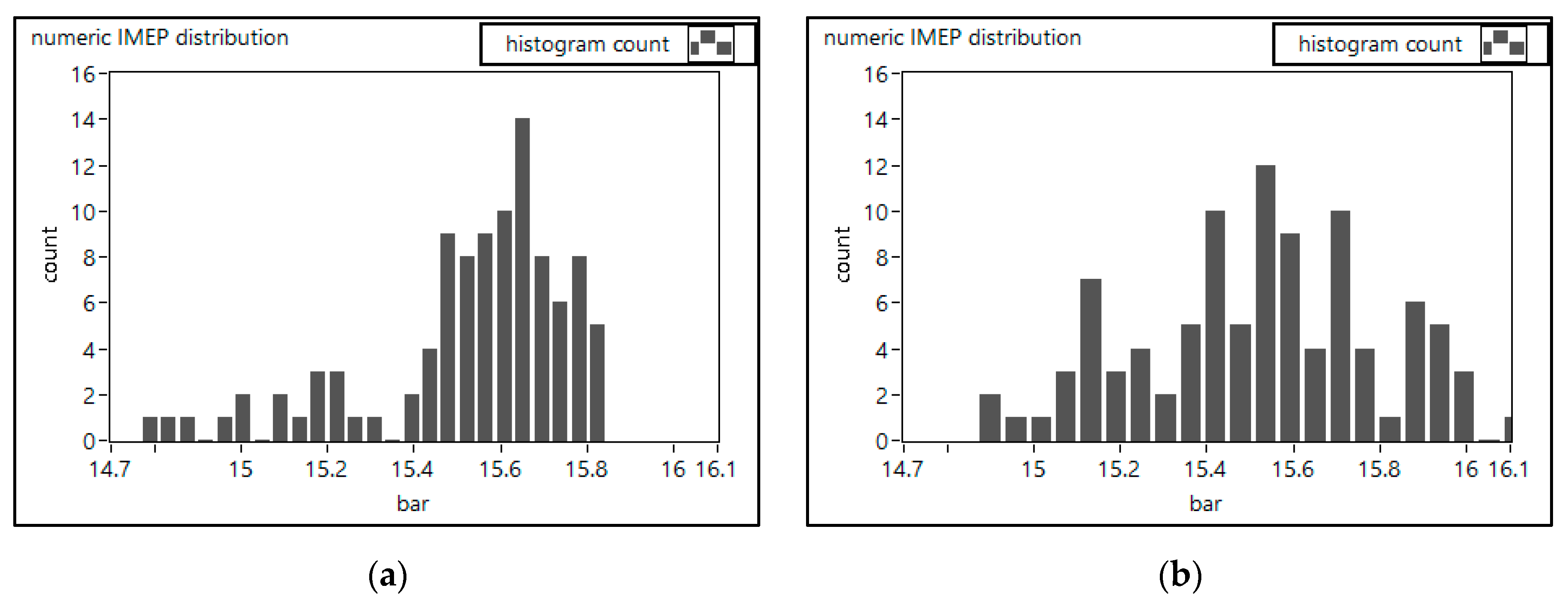
Figure 18.
Histogram of numeric IMEP distribution; MAP = 1.6 bar, n = 2500 rpm, fuel NG. (a) Hill function, (mean value = 15.5 bar, SD = 0.236 bar); (b) Wiebe function, (mean value = 15.5 bar, SD = 0.292 bar).
Figure 18.
Histogram of numeric IMEP distribution; MAP = 1.6 bar, n = 2500 rpm, fuel NG. (a) Hill function, (mean value = 15.5 bar, SD = 0.236 bar); (b) Wiebe function, (mean value = 15.5 bar, SD = 0.292 bar).
Table 1.
Engine technical features.
Table 1.
Engine technical features.
| Engine Specification | Value |
|---|
| Number of intake valves per cylinder | 1 |
| Number of exhaust valves per cylinder | 1 |
| Cylinders | 4 |
| Stroke | 78.86 (mm) |
| Bore | 70.8 (mm) |
| Rod/crank ratio | 3.27 |
| Compression ratio | 9.8 |
| Engine displacement | 1242 (cm3) |
| Gasoline port fuel injector | Bosch, model EV6 |
| Natural Gas port fuel injector | Bosch, model EV1 |
Table 2.
Operating conditions tested.
Table 2.
Operating conditions tested.
| Operating Condition | Value |
|---|
| Manifold air temperature | 28 ± 10 (°C) |
| Manifold Absolute Pressure | 1 bar, 1.2 bar, 1.4 bar, 1.6 bar |
| Speed of the engine | 1500, 2000, 2500, 3000, 3500, 4000, 4500, 5000 (rpm) |
| Spark advance | maximum brake torque value |
| fuel to air ratio | Stoichiometric |
| Natural Gas ratio in the fuel mixture | 80%, 60%, 40% |
Table 3.
Average calibration coefficients for all the fuel mixtures.
Table 3.
Average calibration coefficients for all the fuel mixtures.
| Fuel Mixture | a (Wiebe) | m (Wiebe) | δ (Hill) | n (Hill) |
|---|
| 40% NG | 22.6 | 2.40 | 35.8 | 4.86 |
| 60% NG | 23.1 | 2.38 | 36.3 | 4.80 |
| 80% NG | 20.3 | 2.30 | 35.7 | 4.69 |
| 100% NG | 19.0 | 2.31 | 36.9 | 4.78 |
Table 4.
Experimental and simulated IMEP with absolute prediction errors (40% NG; MAP = 1 bar).
Table 4.
Experimental and simulated IMEP with absolute prediction errors (40% NG; MAP = 1 bar).
| Engine Speed [rpm] | Spark Advance [CAD BTDC] | Engine IMEP [bar] | Hill IMEP [bar] | Wiebe IMEP [bar] | Hill abs. Error % | Wiebe abs. Error % |
|---|
| 1500 | 20 | 8.399 | 8.277 | 8.396 | 1.5 | 0.0 |
| 2000 | 24 | 8.500 | 8.567 | 8.581 | 0.8 | 1.0 |
| 2500 | 27 | 9.037 | 9.097 | 9.218 | 0.7 | 2.0 |
| 3000 | 28 | 9.408 | 9.401 | 9.360 | 0.1 | 0.5 |
| 3500 | 29 | 9.338 | 9.593 | 9.556 | 2.7 | 2.3 |
| 4000 | 26 | 8.925 | 8.974 | 9.189 | 0.5 | 3.0 |
| 4500 | 26 | 8.843 | 8.800 | 9.046 | 0.5 | 2.3 |
| 5000 | 25 | 7.883 | 8.099 | 8.156 | 2.7 | 3.5 |
| | | | | mean value | 1.2 | 1.8 |
Table 5.
Experimental and simulated IMEP with absolute prediction errors (40% NG; MAP = 1.2 bar).
Table 5.
Experimental and simulated IMEP with absolute prediction errors (40% NG; MAP = 1.2 bar).
| Engine Speed [rpm] | Spark Advance [CAD BTDC] | Engine IMEP [bar] | Hill IMEP [bar] | Wiebe IMEP [bar] | Hill abs. Error % | Wiebe abs. Error % |
|---|
| 1500 | 15 | 10.942 | 10.749 | 11.064 | 1.8 | 1.1 |
| 2000 | 20 | 11.262 | 11.223 | 11.356 | 0.3 | 0.8 |
| 2500 | 20 | 11.521 | 11.563 | 11.640 | 0.4 | 1.0 |
| 3000 | 23 | 11.789 | 11.926 | 11.960 | 1.2 | 1.5 |
| 3500 | 24 | 11.824 | 11.721 | 12.002 | 0.9 | 1.5 |
| 4000 | 23 | 11.007 | 11.219 | 11.523 | 1.9 | 4.7 |
| 4500 | 23 | 10.624 | 10.928 | 11.195 | 2.9 | 5.4 |
| 5000 | 19 | 8.088 | 8.513 | 8.654 | 5.3 | 7.0 |
| | | | | mean value | 1.8 | 2.9 |
Table 6.
Experimental and simulated IMEP with absolute prediction errors (40% NG; MAP = 1.4 bar).
Table 6.
Experimental and simulated IMEP with absolute prediction errors (40% NG; MAP = 1.4 bar).
| Engine Speed [rpm] | Spark Advance [CAD BTDC] | Engine IMEP [bar] | Hill IMEP [bar] | Wiebe IMEP [bar] | Hill abs. Error % | Wiebe abs. Error % |
|---|
| 1500 | 16 | 12.637 | 12.447 | 12.731 | 1.5 | 0.7 |
| 2000 | 17 | 13.064 | 13.093 | 13.364 | 0.2 | 2.3 |
| 2500 | 15 | 13.114 | 13.262 | 13.442 | 1.1 | 2.5 |
| 3000 | 17 | 13.879 | 13.945 | 14.162 | 0.5 | 2.0 |
| 3500 | 20 | 13.445 | 13.558 | 13.965 | 0.8 | 3.9 |
| 4000 | 22 | 12.999 | 13.097 | 13.158 | 0.8 | 1.2 |
| 4500 | 21 | 12.587 | 12.849 | 13.090 | 2.1 | 4.0 |
| 5000 | 23 | 11.930 | 12.046 | 12.303 | 1.0 | 3.1 |
| | | | | mean value | 1.0 | 2.5 |
Table 7.
Experimental and simulated IMEP with absolute prediction errors (40% NG; MAP = 1.6 bar).
Table 7.
Experimental and simulated IMEP with absolute prediction errors (40% NG; MAP = 1.6 bar).
| Engine Speed [rpm] | Spark Advance [CAD BTDC] | Engine IMEP [bar] | Hill IMEP [bar] | Wiebe IMEP [bar] | Hill abs. Error % | Wiebe abs. Error % |
|---|
| 1500 | 11 | 14.428 | 13.427 | 14.052 | 6.9 | 2.6 |
| 2000 | 12 | 15.056 | 14.820 | 15.093 | 1.6 | 0.2 |
| 2500 | 15 | 15.654 | 15.551 | 15.897 | 0.7 | 1.6 |
| 3000 | 14 | 15.799 | 15.386 | 16.099 | 2.6 | 1.9 |
| 3500 | 17 | 15.571 | 15.510 | 15.762 | 0.4 | 1.2 |
| 4000 | 18 | 14.723 | 14.902 | 15.122 | 1.2 | 2.7 |
| 4500 | 19 | 14.211 | 14.452 | 14.887 | 1.7 | 4.8 |
| 5000 | 19 | 13.003 | 13.380 | 13.506 | 2.9 | 3.9 |
| | | | | mean value | 2.2 | 2.4 |
Table 8.
Experimental and simulated IMEP with absolute prediction errors (60% NG; MAP = 1 bar).
Table 8.
Experimental and simulated IMEP with absolute prediction errors (60% NG; MAP = 1 bar).
| Engine Speed [rpm] | Spark Advance [CAD BTDC] | Engine IMEP [bar] | Hill IMEP [bar] | Wiebe IMEP [bar] | Hill abs. Error % | Wiebe abs. Error % |
|---|
| 1500 | 24 | 7.785 | 7.977 | 8.089 | 2.5 | 3.9 |
| 2000 | 28 | 8.086 | 8.033 | 8.187 | 0.7 | 1.2 |
| 2500 | 28 | 8.702 | 8.645 | 8.795 | 0.7 | 1.1 |
| 3000 | 28 | 9.063 | 8.979 | 9.040 | 0.9 | 0.3 |
| 3500 | 30 | 8.951 | 8.759 | 8.965 | 2.1 | 0.2 |
| 4000 | 27 | 8.600 | 8.644 | 8.566 | 0.5 | 0.4 |
| 4500 | 22 | 7.755 | 7.890 | 8.181 | 1.7 | 5.5 |
| 5000 | 29 | 7.361 | 7.321 | 7.452 | 0.5 | 1.2 |
| | | | | mean value | 1.2 | 1.7 |
Table 9.
Experimental and simulated IMEP with absolute prediction errors (60% NG; MAP = 1.2 bar).
Table 9.
Experimental and simulated IMEP with absolute prediction errors (60% NG; MAP = 1.2 bar).
| Engine Speed [rpm] | Spark Advance [CAD BTDC] | Engine IMEP [bar] | Hill IMEP [bar] | Wiebe IMEP [bar] | Hill abs. Error % | Wiebe abs. Error % |
|---|
| 1500 | 21 | 10.592 | 10.628 | 10.954 | 0.3 | 3.4 |
| 2000 | 23 | 11.124 | 11.228 | 11.359 | 0.9 | 2.1 |
| 2500 | 25 | 11.191 | 11.238 | 11.496 | 0.4 | 2.7 |
| 3000 | 26 | 11.678 | 11.709 | 11.821 | 0.3 | 1.2 |
| 3500 | 27 | 11.549 | 11.436 | 11.842 | 1.0 | 2.5 |
| 4000 | 26 | 10.976 | 11.068 | 11.329 | 0.8 | 3.2 |
| 4500 | 23 | 9.639 | 9.881 | 10.139 | 2.5 | 5.2 |
| 5000 | 22 | 8.004 | 8.479 | 8.485 | 5.9 | 6.0 |
| | | | | mean value | 1.5 | 3.3 |
Table 10.
Experimental and simulated IMEP with absolute prediction errors (60% NG; MAP = 1.4 bar).
Table 10.
Experimental and simulated IMEP with absolute prediction errors (60% NG; MAP = 1.4 bar).
| Engine Speed [rpm] | Spark Advance [CAD BTDC] | Engine IMEP [bar] | Hill IMEP [bar] | Wiebe IMEP [bar] | Hill abs. Error % | Wiebe abs. Error % |
|---|
| 1500 | 20 | 12.128 | 11.883 | 12.242 | 2.0 | 0.9 |
| 2000 | 20 | 13.167 | 12.912 | 12.924 | 1.9 | 1.8 |
| 2500 | 20 | 13.722 | 13.734 | 14.294 | 0.1 | 4.2 |
| 3000 | 21 | 13.418 | 13.620 | 13.815 | 1.5 | 3.0 |
| 3500 | 23 | 13.066 | 13.262 | 13.448 | 1.5 | 2.9 |
| 4000 | 20 | 11.935 | 12.448 | 12.739 | 4.3 | 6.7 |
| 4500 | 22 | 10.519 | 10.793 | 10.962 | 2.6 | 4.2 |
| 5000 | 20 | 8.605 | 9.265 | 9.534 | 7.7 | 10.8 |
| | | | | mean value | 2.7 | 4.3 |
Table 11.
Experimental and simulated IMEP with absolute prediction errors (60% NG; MAP = 1.6 bar).
Table 11.
Experimental and simulated IMEP with absolute prediction errors (60% NG; MAP = 1.6 bar).
| Engine Speed [rpm] | Spark Advance [CAD BTDC] | Engine IMEP [bar] | Hill IMEP [bar] | Wiebe IMEP [bar] | Hill abs. Error % | Wiebe abs. Error % |
|---|
| 1500 | 16 | 14.344 | 14.037 | 14.304 | 2.1 | 0.3 |
| 2000 | 19 | 15.099 | 15.087 | 15.199 | 0.1 | 0.7 |
| 2500 | 20 | 15.383 | 15.350 | 15.720 | 0.2 | 2.2 |
| 3000 | 19 | 15.759 | 15.652 | 15.987 | 0.7 | 1.4 |
| 3500 | 21 | 15.459 | 15.355 | 15.730 | 0.7 | 1.8 |
| 4000 | 18 | 13.288 | 13.906 | 14.175 | 4.7 | 6.7 |
| 4500 | 23 | 13.733 | 13.889 | 14.454 | 1.1 | 5.3 |
| 5000 | 20 | 11.689 | 12.274 | 12.483 | 5.0 | 6.8 |
| | | | | mean value | 1.8 | 3.1 |
Table 12.
Experimental and simulated IMEP with absolute prediction errors (80% NG; MAP = 1 bar).
Table 12.
Experimental and simulated IMEP with absolute prediction errors (80% NG; MAP = 1 bar).
| Engine Speed [rpm] | Spark Advance [CAD BTDC] | Engine IMEP [bar] | Hill IMEP [bar] | Wiebe IMEP [bar] | Hill abs. Error % | Wiebe abs. Error % |
|---|
| 1500 | 21 | 7.760 | 7.843 | 7.861 | 1.1 | 1.3 |
| 2000 | 26 | 7.694 | 7.705 | 7.765 | 0.1 | 0.9 |
| 2500 | 26 | 8.324 | 8.384 | 8.659 | 0.7 | 4.0 |
| 3000 | 26 | 8.800 | 8.670 | 9.012 | 1.5 | 2.4 |
| 3500 | 27 | 8.360 | 8.764 | 8.714 | 4.8 | 4.2 |
| 4000 | 26 | 8.139 | 8.147 | 8.234 | 0.1 | 1.2 |
| 4500 | 26 | 7.672 | 7.569 | 7.680 | 1.3 | 0.1 |
| 5000 | 26 | 7.655 | 7.680 | 7.911 | 0.3 | 3.3 |
| | | | | mean value | 1.3 | 2.2 |
Table 13.
Experimental and simulated IMEP with absolute prediction errors (80% NG; MAP = 1.2 bar).
Table 13.
Experimental and simulated IMEP with absolute prediction errors (80% NG; MAP = 1.2 bar).
| Engine Speed [rpm] | Spark Advance [CAD BTDC] | Engine IMEP [bar] | Hill IMEP [bar] | Wiebe IMEP [bar] | Hill abs. Error % | Wiebe abs. Error % |
|---|
| 1500 | 19 | 10.157 | 9.758 | 10.269 | 3.9 | 1.1 |
| 2000 | 20 | 10.618 | 10.519 | 10.597 | 0.9 | 0.2 |
| 2500 | 24 | 10.905 | 10.967 | 11.064 | 0.6 | 1.5 |
| 3000 | 23 | 11.312 | 11.343 | 11.371 | 0.3 | 0.5 |
| 3500 | 25 | 10.742 | 10.943 | 10.888 | 1.9 | 1.4 |
| 4000 | 28 | 10.313 | 10.625 | 10.557 | 3.0 | 2.4 |
| 4500 | 28 | 9.998 | 10.139 | 10.158 | 1.4 | 1.6 |
| 5000 | 27 | 8.016 | 8.261 | 8.362 | 3.1 | 4.3 |
| | | | | mean value | 1.9 | 1.6 |
Table 14.
Experimental and simulated IMEP with absolute prediction errors (80% NG; MAP = 1.4 bar).
Table 14.
Experimental and simulated IMEP with absolute prediction errors (80% NG; MAP = 1.4 bar).
| Engine Speed [rpm] | Spark Advance [CAD BTDC] | Engine IMEP [bar] | Hill IMEP [bar] | Wiebe IMEP [bar] | Hill abs. Error % | Wiebe abs. Error % |
|---|
| 1500 | 20 | 11.860 | 11.648 | 11.966 | 1.8 | 0.9 |
| 2000 | 21 | 12.959 | 12.869 | 13.065 | 0.7 | 0.8 |
| 2500 | 22 | 13.281 | 13.130 | 13.272 | 1.1 | 0.1 |
| 3000 | 22 | 13.375 | 13.255 | 13.656 | 0.9 | 2.1 |
| 3500 | 23 | 13.005 | 12.974 | 13.165 | 0.2 | 1.2 |
| 4000 | 26 | 12.363 | 12.506 | 12.743 | 1.2 | 3.1 |
| 4500 | 25 | 11.299 | 11.375 | 11.675 | 0.7 | 3.3 |
| 5000 | 23 | 9.459 | 9.730 | 10.026 | 2.9 | 6.0 |
| | | | | mean value | 1.2 | 2.2 |
Table 15.
Experimental and simulated IMEP with absolute prediction errors (80% NG; MAP = 1.6 bar).
Table 15.
Experimental and simulated IMEP with absolute prediction errors (80% NG; MAP = 1.6 bar).
| Engine Speed [rpm] | Spark Advance [CAD BTDC] | engine IMEP [bar] | Hill IMEP [bar] | Wiebe IMEP [bar] | Hill abs. Error % | Wiebe abs. Error % |
|---|
| 1500 | 20 | 13.886 | 13.884 | 14.144 | 0.0 | 1.9 |
| 2000 | 20 | 14.782 | 14.819 | 14.946 | 0.3 | 1.1 |
| 2500 | 22 | 15.172 | 15.132 | 15.397 | 0.3 | 1.5 |
| 3000 | 22 | 15.660 | 15.487 | 15.610 | 1.1 | 0.3 |
| 3500 | 24 | 15.133 | 15.076 | 15.338 | 0.4 | 1.4 |
| 4000 | 25 | 14.340 | 14.585 | 14.741 | 1.7 | 2.8 |
| 4500 | 26 | 13.348 | 13.224 | 13.609 | 0.9 | 2.0 |
| 5000 | 27 | 12.621 | 12.804 | 12.891 | 1.4 | 2.1 |
| | | | | mean value | 0.8 | 1.6 |
Table 16.
Experimental and simulated IMEP SD.
Table 16.
Experimental and simulated IMEP SD.
| Operating Condition | Experimental IMEP SD [bar] | Simulated IMEP SD (Hill) [bar] | Error % Simulated Hill vs. Experimental | Simulated IMEP SD (Wiebe) [bar] | Error % Simulated Wiebe vs. Experimental |
|---|
| n = 3500 rpm MAP = 1 bar | 0.214 | 0.222 | 3.74% | 0.206 | −3.74% |
| n = 2500 rpm MAP = 1.6 bar | 0.239 | 0.236 | −1.26% | 0.292 | 22.2% |


