Abstract
Oversimplifying occupant behaviour using static and standard schedules has been identified as a limitation of building energy simulation tools. This paper describes the use of hierarchical cluster analysis to establish the most typical indoor temperature profiles of Albanian dwellings based on monitored indoor temperatures in winter and summer, along with building and occupant surveys undertaken in 49 randomly selected dwellings in Tirana. Three statistically different profiles were developed for each summer and winter, indicating that homes are used in different ways, as well as revealing possible comfort requirements. Furthermore, statistical analysis was undertaken to determine the strength of the association between the clusters and contextual factors related to the building, household, and occupancy. A statistically significant association was found between the presence of children and the clusters in winter, suggesting that families with dependents use more energy. Building-related factors including building type, building age, and wall insulation were found to be statistically significantly associated with clusters in summer. These profiles could provide more accurate outcomes of energy consumption of Albanian homes and energy savings from retrofits. They could also facilitate the development of low-energy strategies and policies for specific households.
1. Introduction
Buildings’ energy simulations are one of the most common methods for estimating the energy demand of existing buildings, as well as energy savings from retrofitting projects [1]. However, there is often a significant discrepancy between the predicted and actual energy consumption of buildings [2,3,4,5,6,7,8,9,10,11,12], which is influenced by different factors and is largely caused by the complex interdependencies that occur between the fabric, services, controls, and occupant behaviour [13,14]. The physical design factors such as building features and the effect of external weather are the focus of many building simulation tools, while it has been challenging to incorporate the interaction between occupants and buildings, even though there has been significant research on occupant behaviours in buildings in recent years [11]. Only 5 out of 27 factors that were suggested in previous studies reviewed by Wei, Jones and de Wilde [15], i.e., room type, occupancy, indoor relative humidity, outdoor climate, and time of day, have been used to model space-heating behaviour in building performance simulations (BPS). Generally, occupant behaviour is oversimplified and predefined through static schedules in building performance simulations, ignoring its stochastic nature, dynamics, and diversity [16]. Improving assumptions about building operation has been a key challenge in recent research [1,17,18,19].
The choice of setpoints and operation schedules used by the building simulation modeler is found to be one of the key factors in the performance gap [20]. Using a sensitivity analysis, Firth et al. [21] found that the predicted energy consumption widely varied with different input parameters, where some of the determining factors of residential space heating demand were the characteristics and usage patterns of heating systems, including setpoint temperature and heating duration. Kelly et al. [22] found a statistically significant effect of setpoints on internal temperatures. Dodoo et al. [23] also found that the indoor air temperature significantly influenced the performance of energy efficiency measures. Wei et al. [24] argued that specifying the user’s heating activity on the energy simulations as active when in reality it is passive results in a great overestimation of the energy saving potential of a retrofitting strategy. The authors of [18,25] have also claimed that the focus is on when occupants are active rather than just present in the house.
The analysis undertaken in this study also shows that despite occupants being at home, it does not necessarily mean that the heating or cooling is on. In this context, the aim of this paper is to develop the most typical indoor temperature profiles that can be used as baseline energy models developed to estimate the energy consumption of homes in Albania, as well as to closely estimate energy savings for future energy retrofitting programs. Hierarchical cluster analysis is used in this study to develop the most typical indoor temperature profiles, as one of the most used statistical analysis methods used previously in the development of occupancy, heating, and indoor temperature profiles [26,27,28,29,30,31]. Belaïd, Ranjbar, and Massié [32] have also used Ascending Hierarchical Classification to define French housing stock profiles based on 1400 dwelling representatives of the French residential sector, aiming to explore the cost-effectiveness of the energy efficiency implementation measures in the residential sector. The same method was used by Huebner et al. [31] in their study of 275 dwellings. Buttitta, Turner, and Finn [33] used an approach based on a statistical clustering technique to generate the representative UK occupancy profiles based on the amount of time spent at home by all occupants of the same household, resulting in 22 different occupancy profiles on weekdays and 24 on weekends, each assigned with the percentage of households with similar occupancy profiles for each dwelling type characterised by specific characteristics. They used k-means clustering as the mains metho of their statistical analysis in order to develop occupancy clusters, which is one of the two broad categories in which traditional clustering methods fall [30]. The other category is hierarchical clustering, used in this study, which is mainly used to develop clusters from small datasets. Although the sample size in this research is small (N = 49) compared to their study (6500 households), it will still provide an insight into the most typical indoor temperature profiles, which can be used for modelling the energy consumption of homes in Albania. Moreover, the hierarchical clustering method used in this research is mainly used for the clustering technique in small datasets.
Three statistically significantly different indoor temperature clusters were developed based on recorded indoor temperatures of 49 dwellings in Tirana, Albania. The analysis extends to finding associations between the identified clusters and buildings, households, and occupancy factors to understand the most important factors that drive indoor temperatures in both winter and summer. Andersen, Fabi, and Corgnati [34] also underline the importance of occupants’ socio-demographics and household characteristics in order to identify specific target groups for energy-saving policy programmes and retrofit options. This approach therefore addresses the performance gap by considering various indoor temperature profiles rather than a default temperature setpoint contributing towards more user-centred approach to retrofits, as well as future programmes and policies, as has also been suggested by Ben and Steemers [35].
1.1. Influence of Occupant Behaviour in Building Energy Simulations
It is widely recognised that occupant behaviour has a significant impact on building energy demand and on indoor thermal comfort conditions [4,9,14,36,37]. Nonetheless, integrating occupant behaviour into building energy simulations has been found to be challenging [11], as it is usually oversimplified and predefined through static schedules in building performance simulations [9,37,38,39,40,41]. Due to a lack of pre-retrofit evaluation in the early stage of the design and a lack of data about various aspects of the building, considerable assumptions and predictions are used [42,43,44]. Therefore, the improvement of occupants’ presence and modelling their actions in building simulations is essential to enhance the accuracy of the building energy simulation process [12]. Yao and Steemers [45] claimed that the number of occupants and the length of the period in which the dwelling is occupied are the main factors influencing energy consumption. Yan et al. [12] also found that occupant–building interaction is affected by the arrival, departure, and duration of absence of occupants. Jia, Srinivasan, and Raheem [11] described how occupant presence/absence in rooms is not enough for occupant behaviour modelling and how further information is needed regarding the adaptation to the indoor environment and the occupants themselves.
In fact, indoor air temperature has been found to significantly influence the performance of energy-efficiency measures [23], and assuming one standard indoor temperature profile for energy modelling for all homes would contribute to the performance gap between the actual and estimate energy consumption in homes. Developing various indoor temperature profiles would overcome this assumption and would assist in better calculations of energy consumption in homes as well as closer predictions of energy savings through energy retrofitting.
However, indoor temperature is highly affected by occupant behaviour, which itself can be affected by various factors, including a building’s characteristics, social and personal characteristics, rebound effects, personal comfort, lifestyle and cultural background, occupants’ knowledge and skills, and occupants’ experience [46]. According to [47,48], there are also social-psychological factors that may influence thermal comfort and energy behaviours, including beliefs, values, norms, social trust, habits, energy saving attitudes, motivations, perceived behavioural control, and environmental concerns. Furthermore, Ortiz, Itard, and Bluyssen [49] support the claim that occupant behaviours are interplays of personal, environmental, and social factors and that their actions are influenced by the way the occupants understand energy, control, and comfort. Ebrahimigharehbaghi et al. [50] considers the multiple origins of the factors that influence occupant behaviour and categorises them as: motivations, barriers, and contextual and personal factors. Fabi et al. [51] classified these factors into five groups: physical environmental factors, contextual factors, psychological factors, physiological factors, and social factors. Tam, Almeida, and Le [52] grouped the factors influencing occupant behaviour into objective factors, including environmental conditions such as temperature, air velocity, climate, and noise, and subjective factors, which depend on the personal perception of comfort and are affected by age, metabolic activity, particular mood, habits, sensations, and social interaction. According to Schaffrin and Reibling [53], all forms of consumption energy practices demonstrate lifestyle choices and can be a form of self-expression.
In this context, to investigate the effect of occupant behaviour in indoor temperature in homes, this study investigates the association of indoor temperature profiles with socio-demographic characteristics (education level, household size, presence of children or retired persons, income, and monthly energy bill), as well as behavioural factors (cooling and heating usage patterns during the day and night) for each household selected, along with the effect of building characteristics (building type and size, period of construction, existence of wall insulation or double glazing, and type of heating or cooling).
1.2. Review of Factors Affecting Indoor Temperatures in Dwellings
Indoor temperature has been found to significantly influence the performance of energy retrofits [23]. The setpoint temperature for heating and the duration of the heating period are the greatest influential factors on energy consumption for space heating in homes [21,54,55,56,57,58]. An increase in energy consumption of 10% has been calculated for each degree of indoor temperature in a study undertaken by Tommerup, Rose, and Svendsen [59] on single-family houses in Denmark. Peng et al. [60] found significant variations in building performance using three classifications of occupant behaviours based on an air-conditioning operation schedule, indoor temperature preference, and household loads based on the division type. Bruce-Konuah, Jones, and Fuertes [61] found that physical environmental variables, including indoor and outdoor temperature, indoor relative humidity, and solar radiation, affect occupants’ behaviour in terms of manual space heating override during the heating season. They found an average increase in space heating energy consumption of 21.5% and 13.6% on weekday and weekend, respectively. There are also other factors that may lead to indoor temperature profiles differing from heating demand profiles [31], and having distinct temperature profiles would indicate not only that homes are used in different ways by different occupants, but could also indicate various comfort requirements. Kelly et al. [22] developed a model to predict the daily mean internal temperatures for a national building stock and found behavioural and socio-demographic properties of the occupants’ significant variables among physical properties of the building, the external climate, and dwelling’s geographic location to explain internal temperature demand. Hunt and Gidman [62], using a national field survey of house temperatures in the UK, found that a household’s income was a strong indicator of room temperature, with lower-income homes found to be 3 °C lower on average in the heating season.
Notwithstanding the many uncertainties, default assumptions about how homes are heated and cooled, and at what temperatures, have been used for modelling energy consumption of housing stock [17]. Heating temperatures of 21 °C have been assumed for modelling of housing stock and estimating energy savings from retrofitting strategies in the UK [63]. Al-Mumin, Khattab, and Sridhar [64] found a variation in thermostat setpoints from below 19 °C to above 25 °C after investigating summer air-conditioning use in residential buildings. Moreover, Peng et al. [60] found that air-conditioning operation within a household varied every day. Default setpoint temperatures of 20 °C and 26 °C for heating and cooling, respectively, have been used in a study of energy retrofitting of residential stock in Albania [65]. This assumption leads to energy consumption and energy saving estimations largely different from the actual ones [31].
Notwithstanding that the heating setpoint effect has been largely acknowledged as one of the main factors that affects the interaction between the occupants and the building, there is still no standard method to assign the heating setpoint for building simulation [1]. Therefore, developing temperature profiles would decrease the estimations coming from the use of a single heating and cooling setpoints, as well as the default heating and cooling duration in homes.
2. Materials and Methods
A mixed-method approach combining qualitative and quantitative research methods was used to provide a more comprehensive understanding of the topic under investigation. The methodology for this study comprised two principal steps:
- Data collection, including indoor temperature monitoring and surveys of 49 randomly selected dwellings to evaluate the actual energy use in case studies representing the main Albanian building types.
- Data analysis, including cluster analysis, leading to the identification of clusters and relationships between clusters and contextual factors.
2.1. Data Collection
The data collection methods included the following:
- Building surveys to gather information on the buildings’ properties and energy use. Quantitative data were collected regarding building materials and construction, orientation, floor area, appliances, and lighting, which allowed for a detailed picture of energy use and behaviours within the home. Electricity bills were also obtained.
- Occupants’ survey to collect socio-demographic information, as well as to obtain an insight into how and when the house is used, occupants’ attitudes and habits, and other everyday practices in their home. Setpoint temperatures and duration of heating periods were recorded from each occupant’s responses. The study adopted the method of questionnaire-guided interviews as the most appropriate technique for gathering all essential information in its full range and depth, as well as for obtaining insights into occupant behaviour. Only one occupant per dwelling participated in the survey to provide consistency across the research.
- Continuous monitoring of indoor temperature in the living room and main bedroom was also conducted for six weeks in summer (30 June to 12 August) and winter (5 January to 16 February) to assess the indoor environment in the house. Only the indoor temperature was monitored during the field studies in order to indicate the range of temperature present within homes. The focus of this research was not conducting a thermal comfort field study, but to gain an insight into how people evaluate their home and how it was really performing.
Sample Characteristics
Forty-nine dwellings of various building typologies were randomly selected in urban and rural areas of Tirana. Most of the sample comprises flats and detached houses. Differences in construction techniques used in Albanian residential buildings built pre-1990 and post-1991 are also reflected in the sample. All the dwellings built post-1991 were constructed using a concrete structural loading scheme with no-loading hollow bricks or blocks external walls, while pre-fabricated panels and solid brick walls with higher thermal mass were very common constructions in buildings built pre-1990. Electricity was the most common type of energy used for space heating, mainly due to lack of infrastructure or security for using other types such as gas and wood. On the other hand, electricity is widely used for cooling during the hot season. Main characteristics of the sample are given in Table 1.

Table 1.
Frequency of different characteristics in the sample.
2.2. Data Analysis
2.2.1. Descriptive Analysis of the Measured Indoor Temperatures during Summer and Winter
After statistically exploring all datasets for normality through exploring statistics, histograms, outliers, normal Q-Q plots, and detrended normal Q-Q, we decided to clean the dataset in terms of the extreme outliers to minimise the skewness of the data distribution. Outliers were not removed from the dataset, as they were not unusual for the period of monitoring. One-sample T-test was undertaken for each variable to check whether the mean temperature of each living room statistically significantly differed from before removing the extreme outliers. A statistically non-significant difference was found (p > 0.05) for each of the dwellings. The mean daily indoor temperature was then calculated for both the living room and the bedroom of each dwelling. The hourly mean temperature was also calculated for each hour to investigate the temperature profile during the day.
2.2.2. Cluster Analysis and Statistical Tests
Due to the high variability in indoor temperatures recorded in the sample, a hierarchical cluster analysis was conducted to limit the number and determine the most typical profiles of indoor temperatures of Albanian homes using the data collected. Hierarchical cluster analysis is an exploratory data tool for organising data into meaningful groups by maximising the similarity of cases within each cluster and maximising dissimilarities between groups that are not previously known [66]. This means that the dwellings are grouped into clusters based not on the building’s characteristics, but on the way that homes are used, and the indoor temperature profiles of dwellings within the same cluster are as similar to each other as possible.
Cluster analysis a statistical analysis method used in previous studies to determine occupancy and heating profiles [26,27,28,29,30], as well as indoor temperature profiles in living rooms [31]. There are two main cluster analysis methods, k-means and hierarchical. Hierarchical analysis was chosen over k-means because it is mostly used for small datasets, and the number of clusters created is determined after plotting the distances between each data point. In contrast, k-means is used more for large datasets and the number of clusters is decided before plotting the dataset. For hierarchical clustering, other studies suggest that a minimum of 10 observations in each cluster should be considered [30,31,67]. The indoor temperature profiles delivered from the cluster analysis undertaken in this paper, together with the occupants’ surveys in summer and winter, were the main sources for developing indoor temperature profiles of Albanian homes.
Clusters were created based on the centralised temperatures, meaning that the average of each data point measurement was calculated for each day and then across the six weeks for each dwelling in summer and winter. Using the SPSS 24 statistical package, a hierarchical cluster analysis was performed with an agglomeration schedule and Ward’s method, which uses the f-value to maximise the significance of differences between clusters. Because the dataset is made of interval data, square Euclidean distance was chosen as the distance measure. Variables (each weekday and the weekend) were standardised to Z-scores, so they all contribute equally to the distance or similarity between cases. Finally, clusters for both summer and winter were described by testing the differences in several buildings, socio-demographics, and occupant behaviour factors, using chi-square tests and one-way ANOVA tests for categorical and continuous variables, respectively. When the results are statistically significant (p > 0.05), this shows that there is a significant association between that building/socio-demographic/behaviour factor and the clusters. However, the chi-squared test only shows if there is an association or not between the two variables but does not give the strength of the association. For this purpose, the phi coefficient can be used, and because tables were larger than 2 by 2, Cramer’s V were used in this analysis [66].
Fundamentally, the analysis still provide an insight into the most typical indoor temperature profiles, which can be used for energy models of Albanian housing stock, allowing for better energy estimations and predictions, which are closely related to occupant behaviours.
3. Results
3.1. Descriptive Statistics of Indoor Temperatures in Summer and Winter
The summer field study involved the monitoring of the indoor temperature of 49 living rooms from 30 June to 12 August at half-hourly intervals to cover the hottest season of the year in the Albanian climate. The outdoor temperature ranged from 19.6 °C to 41.1 °C, while the indoor temperature ranged from 19.5 °C to 37 °C. The indoor temperature is well above the recommended temperature of 20 °C, considered as the comfortable temperature in living rooms by Albanian regulation [68], as shown in Figure 1.
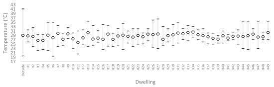
Figure 1.
Minimum, maximum, and mean temperatures in living rooms of each monitored dwelling during the summer.
The house with the lowest indoor temperature (H11) in the sample still had indoor temperatures above 25 °C for more than 80% of the day. Furthermore, 37 dwellings experienced temperatures over 28 °C for more than 50% of the day. This clearly demonstrates that all dwellings in the sample are overheated during the summer.
Monitoring of the same dwellings from 5 January to 16 February at half-hourly intervals covered the coldest season of the year in the Albanian climate. The outdoor temperature ranged between −5.5 °C and 18.5 °C, while the indoor temperature ranged from −6 °C to 29.5 °C in living rooms. The actual indoor temperatures for living rooms during the monitoring time are shown in Figure 2. Elevated temperature variations were also observed. For some of the dwellings temperatures close to the outdoor temperature were recorded, meaning that they had little or no heating at all and/or that windows may have been left open during the day.
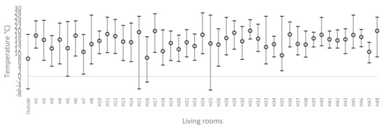
Figure 2.
Minimum, maximum, and mean temperatures in living rooms of each monitored dwelling during the winter.
Hourly Profiles of Indoor Temperatures in Summer and Winter
To investigate the temperature profile during the day, the mean hourly temperatures of living rooms in summer and winter were calculated, as shown in Figure 3. Each line represents the mean hourly temperature of the selected dwellings, while the bold red line represents the mean outdoor temperature during the same period of monitoring. In summer, all the dwellings had a continuous mean indoor temperature of above 25 °C throughout the day, and most of them exceeded 28 °C. There is a smaller range of indoor temperatures throughout the day and between dwellings compared to winter, where a higher temperature range is noticeable, as well as various temperature profiles. Hourly profiles that have very low temperature during the day are present, as well as profiles with temperatures above 20 °C. This indicates the large variation of hourly profiles in Albanian dwellings, which could be a result not only of different building properties, but also of different behaviours within the household.
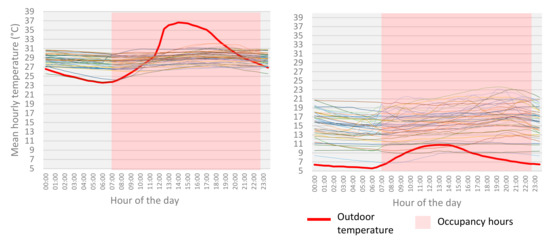
Figure 3.
Mean hourly temperatures in living rooms during the summer (left) and winter (right). (Different colour lines represent the mean hourly temperature of the selected dwellings).
3.2. Cluster Analysis in Summer
Using centralised temperature from the dataset from the summer field study, three clusters were produced using hierarchical clustering and following the rule of each cluster with a minimum of ten observation [30,31,67]. The membership of each cluster is shown in Table 2 and is produced through an agglomeration schedule and Ward’s method, which uses the F-value to maximise the significance of differences between clusters. It is the uneven distribution of the sample into clusters that identifies the most typical indoor temperature profile in Albanian homes. Cluster 1 represents the largest cluster, which comprises over half of the sample (49% in weekend clusters), with an hourly temperature of around 29 °C. Clusters 2 and 3 represent 29% and 20% of the sample (29% and 22% of the sample for weekends), with hourly mean temperatures of 27.5 °C and 30 °C, respectively. Clusters for both weekdays and weekends have been created, which do not differ much from each other in terms of membership. However, further analysis is undertaken to statistically evaluate the differences between them.
Table 2.
Clusters’ membership of the cases for weekdays and weekends in summer.
Figure 4 shows the daily and hourly mean temperatures of each cluster for both weekdays and weekends. All three clusters for both weekdays and weekends have the same sensitivity but in different temperature ranges, and the temperature profiles of weekends are very close to those of weekdays. Cluster 3 follows very closely the mean daily external temperature profile, which indicates that these dwellings might have been cooled for small periods or not at all. Cluster 1, representing most of the dwellings, has a mean daily temperature up to 3 °C lower than the external one during the hottest days of the summer. On the contrary, Cluster 2, which is the second most common cluster in the sample, has temperatures lower than the other two clusters, indicating actions from the occupants to maintain a cooler indoor temperature than in the other cases. The hourly mean temperature tends to be lower in the morning and starts to increase in the early afternoon, reaching a peak in the evening in Clusters 1 and 3 and in the late afternoon in Cluster 2.
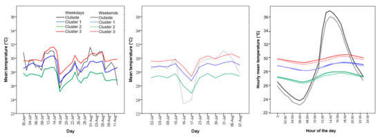
Figure 4.
Mean daily temperature for weekdays (left) and weekends (centre); mean hourly temperature profiles for both weekdays and weekends (right) of the three clusters, together with external temperature.
Statistical analysis was undertaken to determine whether the three clusters are significantly different from each other, which means that they represent three distinctive temperature profiles. To determine the type of statistical test to use (parametric or non-parametric), the assumption of equality of variances has been tested using Levene’s F-test for equality of variances, as shown in Table 3. The test showed non-homogeneity of variances for weekdays (F = 7.2 and p = 0.002) and homogeneity of variances for weekends (F = 1.4 and p = 0.270). Therefore, the Games–Howell test (non-parametric) and Scheffe tests (parametric) were used for post hoc pairwise comparisons for weekdays and weekends, respectively.
Table 3.
Descriptive analysis of the mean temperature of each cluster based on the mean temperature of each dwelling and Levene’s test results in summer.
Both Games–Howell and Scheffe tests undertaken for pairwise comparison between clusters showed significantly different mean temperatures (p = 0.000) between clusters for both weekdays and weekends profiles.
Relationship of Clusters in Summer to Contextual Factors
- Building characteristics
Seven main building-related variables were tested, as shown in Table 3. Each column gives the proportion of households for each value of the variable. Because all the building-related variables were categorical, only chi-squared analysis has been performed, and the results are given in Table 4.
Table 4.
Chi-squared analysis of building variables between clusters in summer.
Cluster 2 had significantly more detached houses (64.3%) than the other two clusters (28% and 34.7%, respectively, for cluster 1 and 3), while Clusters 1 and 3 are equally represented by flats. Moreover, the majority of dwellings in Cluster 2 were constructed post-1991, while most of the dwellings constructed pre-1990 form the membership of Cluster 3. The largest share of dwellings that have both wall insulation and double glazing is in Cluster 2, which in fact had the lowest indoor temperature in terms of mean daily and hourly profiles.
Generally, dwellings in Cluster 1 are smaller (up to three bedrooms) in size than those in the other two clusters. Most of the dwellings in each cluster are air-conditioned; however, the largest share of air-conditioned dwellings is in Cluster 3.
Chi-squared test for independence showed a statistically significant association (p < 0.05) between clusters and building-related factors, such as building type, period of construction, and wall insulation. This means that the clusters are dependent on these factors. No statistically significant association was found between clusters and dwelling size and type of cooling.
Effect size analysis using Cramer’s V was performed for building factors that had a statistically significant association with the clusters, as shown in Table 5. Criteria for determining the effect size are shown in the last three columns. According to Pallant [66], to determine which criteria to use for judging the effect size, whichever of R-1 (subtracting 1 from the number of categories in the row) or C-1 (subtracting 1 from the number of categories in the column) is smaller should be correlated to the values for small, medium, or large effect.
Table 5.
Cramer’s V test results of building variables between clusters in summer.
Building type and the period of construction have a statistically significant large effect on the clusters, while wall insulation, and double glazing have a statistically significant small and medium effect, respectively.
- Socio-demographic factors
Notwithstanding that several studies have shown an association between socio-demographic factors and energy consumption and temperatures, no significant differences between clusters were found in this sample, as shown in Table 6. Cluster 3 has the highest proportion of households with the highest education and single occupancy. Moreover, 70% of households in this cluster have over four members and children. The proportion of households with a retired member is higher in Cluster 3 as well.
Table 6.
Chi-squared analysis of socio-demographic variables between clusters in summer.
For continuous variables, one-way ANOVA, with post hoc tests corrected with Bonferroni, was used to test for difference between clusters. The results are given in Table 7. No statistically significant difference was found in the three clusters in the monthly incomes and electricity bills.
Table 7.
One-way ANOVA test results of continuous socio-demographic variables between clusters in summer.
- Occupant behaviour factors
Two main variables were tested, as shown in Table 8. However, chi-squared tests showed that none of the variables under investigation had a statistically significant association with the clusters. Even though no statistically significant association was found between these factors and the clusters during summer, chi-squared tests are useful to describe the clusters relating to these variables. Most of the households in all three clusters were cooled in the afternoon and in the afternoon and evening. However, Cluster 2 has the largest share of households that cool the space during the night.
Table 8.
Chi-squared analysis of occupant behaviour variables between clusters in summer.
3.3. Cluster Analysis in Winter
Three identical weekday and weekend clusters were created using the hierarchical cluster analysis of the winter indoor temperatures dataset, as shown in Table 9. The same method was followed as for the summer cluster analysis. Cluster 2 represents the largest cluster, with nearly 45% of the sample, and corresponds to the middle range of indoor temperatures of around 15°C. Clusters 1 and 3 represent 33% and 22% of the sample, respectively.
Table 9.
Clusters’ membership of the cases for weekdays and weekends in winter.
Figure 5 shows the daily and hourly mean temperatures of each cluster for both weekdays and weekends. Although both weekdays and weekends have the same membership of dwellings, the profiles are produced using absolute (instantaneous) temperature data, which differ between weekdays and weekends. The daily mean temperature is almost within the same range for both weekdays and weekends for each cluster. It was also observed that dwellings in Cluster 1 had temperatures above 15 °C during the coldest week of the monitoring time, while dwellings in Cluster 3 follow the external temperature profile more closely, indicating that some or all dwellings included in this cluster had little or no heating.
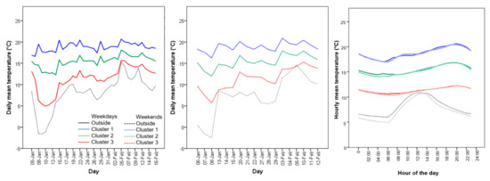
Figure 5.
Mean daily temperature for weekdays (left) and weekends (centre); mean hourly temperature profiles for both weekdays and weekends (right) of the three clusters, together with external temperature.
Regarding hourly mean temperatures, weekday and weekend profiles have almost the same sensitivity as each other for all three clusters. Cluster 1 is characterised by a higher temperature throughout the day compared with the other two clusters. There is a steep rise in temperatures at 7 a.m., and they continue to steadily increase until 10 p.m. However, in Cluster 2, which represents most of the dwellings, there is only a small peak in the morning, and as is the case in Cluster 1, the temperature increases gradually until evening. For weekends in Cluster 2, there is a small peak in temperature in the morning, and the profile is then close to the weekdays’ profile for the rest of the day. On the contrary, Cluster 3 represents the dwellings with the lowest indoor temperature throughout the day. There is almost a flat line throughout the day for both weekday and weekend profiles, with a small peak in the evening. This indicates that these dwellings barely heat the space during the winter.
As in the summer cluster analysis, Levene’s F-test for equality of variance was used. The test showed the homogeneity of variances (p > 0.05) for weekdays and weekends (F = 2.2 and p = 0.130 and F = 3.0 and p = 0.06, respectively). Therefore, Scheffe tests were performed for pairwise comparison between clusters and showed significantly different mean temperatures (p = 0.000) between clusters for both weekday and weekend profiles (see Table 10).
Table 10.
Descriptive analysis of the mean temperature of each cluster based on the mean temperature of each dwelling and Levene’s test results in winter.
Relationship of Clusters in Winter to Contextual Factors
- Building characteristics
A chi-squared test was performed to describe the difference between clusters for categorical variables, with the results given in Table 11. Each column shows the proportion of dwellings for each value of the variable. In total, seven building-related factors were tested.
Table 11.
Chi-squared analysis of building variables between clusters in winter.
There is almost an equal spread of detached houses in the three clusters, while the proportion of flats in Clusters 1 and 2 is bigger than in Cluster 3. On the other hand, mainly semi-detached and terraced houses compose Cluster 3. There is a close representation of both periods of construction in all clusters. However, Clusters 2 and 3 have the highest proportion of pre-1990 and post-1991 dwellings, respectively. The highest proportion of dwellings that had wall insulation and double glazing was in Cluster 1, followed by Cluster 3. It is interesting that a high proportion of dwellings with better thermal properties are associated with Cluster 3, which recorded the lowest indoor temperatures. However, the chi-tests showed no statistically significant association between clusters and thermal properties of the dwellings in winter. Small dwellings are associated more with Clusters 1 and 2, while bigger dwellings were associated with Cluster 3, in which the recorded indoor temperatures are very low and may be related to the high ratio of space volume to heat. Heat pumps were also more popular in Cluster 1.
To summarise, the proportion of dwellings for most of the categories of each tested variable is equally spread between the three clusters, regardless of the building factors. For this reason, chi-squared tests did not find a statistically significant association between clusters and each of the tested building factors. This indicates that there might be other factors that influence the indoor temperatures of dwellings in Albania in winter.
- Socio-demographic factors
Chi-squared tests and one-way ANOVA statistical tests were performed to test the association between clusters and socio-demographic factors for categorical and continuous variables, respectively (see Table 12). Household occupants in all three clusters were found to have similar education levels. Cluster 2 has the highest proportion of small households of up to two occupants and big households of more than three occupants at the same time. The highest proportion of households with children is in Cluster 1, with 90% of all households in this cluster’s membership. In addition, the association between clusters and the presence of a child in the household was found to be statistically significant (p = 0.016). On the contrary, no association was found between clusters and the presence of a retired member in the households. Based on the occupants’ surveys, this might have been associated with the inability to keep adequate thermal comfort because of economic factors in these households.
Table 12.
Chi-squared analysis of socio-demographic factors between clusters in winter.
For continuous variables, one-way ANOVA was used to test for differences between clusters. No statistically significant difference was found in the three clusters for the monthly incomes and electricity bills (see Table 13).
Table 13.
One-way ANOVA test results of continuous socio-demographic variables between clusters in winter.
- Occupant behaviour factors
Two main variables were tested, as shown in Table 14. Chi-squared tests showed that none of the variables under investigation had a statistically significant association with the clusters. In Cluster 1, which was characterised by a daily profile of high temperatures throughout the day and two peaks in the morning and evening, included most of the households that heated the space in the morning and evening. However, more than half of the households turned the heating on at different times during the day, including 13.3% that kept the heating on all day. Almost the same situation can be seen in Cluster 2. On the contrary, most of the households in Cluster 3 heated their home in the afternoon or later, with 40% turning the heating on in the morning and evening, while 10% kept the heating on all day. In all three clusters, 20% of households or less turned the heating on during the night.
Table 14.
Chi-squared analysis of occupants’ behaviours and thermal variables between clusters in winter.
4. Discussion
4.1. Description of Indoor Temperature Profiles
Using the data collected through indoor temperature monitoring and surveys in 49 dwellings in Albania, this study aimed to develop indoor temperature profiles in summer and winter that could be used to assess the energy performance of existing residential buildings in Albania through energy modelling. Due to the high variability of indoor temperatures measured, hierarchical cluster analysis was performed to produce three statistically different clusters each for summer and winter. The clusters were further examined for relationships with a selection of contextual factors related to the building, household, and occupancy. As in other studies [31,69,70], weekday and weekend profiles were distinguished. In this study, a statistically non-significant difference between weekday and weekend profiles was found, suggesting that the building fabric has a high impact on the indoor environment. Very small differences were also found in other studies between weekdays and weekends in terms of average temperatures [70] and heating durations [70,71]. The fact that three significantly different clusters were produced may indicate that homes were used in different ways, which supports findings revealed by many other studies, including [4,9,14,36,37], which emphasised the role of occupant behaviour on indoor environment as well as energy consumption in homes. Furthermore, the different clusters could be associated with various comfort requirements.
An analysis of the clusters shows that the highest membership falls in the middle range of temperatures, suggesting that most occupants heat or cool their dwellings to some extent. However, there is also a high proportion of hardly treated dwellings, with 20% and 33% of the sample in summer and winter, respectively, mostly due to the inability to do so for economic reasons. All clusters in summer have the same sensitivity on the hourly profiles, but in various temperature ranges. They fall in the morning and gradually increase throughout the day until they reach a peak in the evening. In summer, hourly temperatures of around 29 °C, representing Cluster 1, were found in over half of the sample. The temperature profile of Cluster 3 was very close to the external temperature profile and indicates that 20% of the sample cooled the space for short periods or not at all. The fact that temperatures in all profiles did not fall below 26 °C likely indicates that passive natural ventilation at night was barely performed.
The wider range of over 10°C within the day of indoor temperatures in winter was also reflected in the clusters. Cluster 2, with a range of temperatures of around 15 °C, represented nearly 45% of the sample. Similar to the summer clusters, 22% of the sample in winter, represented by Cluster 3, indicated little to no heating due to the closeness of the cluster with the external temperature profile. However, contrary to summer hourly profiles illustrated in the clusters, the hourly profiles in winter did not have the same sensitivity. Cluster 1, which represents 33% of the sample, had a steep rise in temperatures in the morning and fluctuations throughout the afternoon and evening, indicating the use of heating for various periods during the occupied hours. However, Clusters 2 and 3 both had a small peak in the morning and another peak in the evening. However, Cluster 2 had a steady rise in temperatures starting in the afternoon, which indicates the use of heating from the afternoon onwards. As described in [31], indoor temperatures are a substitution of heating and cooling system usage but do not indicate the status of heating or cooling system usage because other factors, such as incidental gains and ventilated heat losses, might also affect the indoor temperature. Cleaning the dataset of extreme outliers and cross-analysing the indoor temperature profiles and results from the occupants’ surveys allowed for the development of a more accurate picture of temperature profiles.
4.2. Contextual Factors Affecting Indoor Temperature Profiles
Statistical tests were performed to find associations between cluster membership and various building, socio-demographic, and behaviour factors for both summer and winter. A statistically significant association was found between clusters in summer and building-related factors such as building type, the period of construction, the archetype, and the wall insulation, with p-values equal to 0.03, 0.021, 0.04 and 0.039, respectively. Shipworth et al. [71] found that detached houses were heated for longer periods than mid-terraced houses, which could be due to more exposed walls in the detached houses, and these houses should therefore be targeted for energy-efficiency improvements. On the other hand, indoor temperatures in flats were found to be higher in winter and summer due to less thermal loss and less cross ventilation in winter and summer, respectively. It is also to be expected that newer constructions with wall insulation and double glazing will have lower indoor temperature during the summer and higher indoor temperatures during the winter. Dwellings that have greater energy efficiency measures have also been found to have higher internal temperatures during winter [57,72]. Other studies have likewise found an association between building-related factors and indoor environments, as well as energy consumption in homes [22,26,31,36,71,72,73].
No statistically significant association was found between the clusters and socio-demographic factors such as education level, household size, and income. However, the presence of children was found to be statistically significant (p = 0.016) for clusters in winter, whereas the presence of retired household members was not found to be statistically significant for both winter and summer. A similar result was found in a study by Zahiri and Elsharkawy [74], which showed that the presence of children had a strong correlation with energy consumption and indoor environment, while less energy was used for heating as the age of occupants increased. Association tests between clusters and occupant behaviour factors, including time of heating/cooling and night heating/cooling in winter and summer, did not show a statistically significant association. However, most of the membership in the cluster with the lowest indoor temperature during the summer and highest indoor temperature during the winter was associated with dwellings that used heating and cooling devices for the highest period of time, as well as night heating/cooling, which suggests irregulated heating/cooling periods in homes. Although some of the associations might not be statistically significant, a chi-squared analysis also described the proportion of each category in each variable’s result. For example, in summer, Cluster 2, which represents the cluster with the lowest hourly temperature profile, comprises mostly detached houses. This suggest that cross ventilation during the summer had a significant effect in maintaining lower temperatures throughout the day.
Temperature clusters developed and examined in this study can be used for distinct temperatures and operation times for each cluster and can subsequently be used in energy simulation tools to estimate the energy demand of residential buildings in Albania, as well as to calculate energy saving estimations from retrofitting projects. Using a single setpoint temperature in energy models has been shown to have a significant discrepancy from the actual energy consumption. A living room heating setpoint temperature of 21 °C and heating operation of 9 and 16 h for weekdays and weekends, respectively, is assumed for living rooms according to BREEDEM models of housing stock in the UK [63], even though the indoor temperatures vary widely to this [55,70]. In a previous study undertaken on the actual energy consumption of building types in Albania [65], the setpoints were assumed to be 20 °C and 26 °C for heating and cooling, respectively. Two options were considered for heating: partial (only one room) and full (the entire dwelling), with both assumed to have the heating on all day, or otherwise correction factors would be applied. However, these assumptions do not consider various occupant behaviours related to different heating or cooling setpoints and durations. Indeed, this study shows that much higher indoor temperatures were recorded in Albanian dwellings during the summer, as well as significantly lower indoor temperatures during the winter compared to the setpoints assumed. Assigning different temperature profiles in energy modelling for dwellings with various building characteristics, as well as various socio-demographic and behaviours of the occupants, would provide a closer estimation of actual energy consumption.
5. Conclusions
Developing indoor temperature profiles for energy models offers a great prospect to minimise the difference between estimated and actual energy consumption, as well as actual energy savings and estimations in the case of retrofits. Three main temperature profiles in summer and winter were developed in this study for weekdays and weekends using hierarchical cluster analysis based on indoor temperatures recorded in both summer and winter in 49 dwellings located in Tirana, Albania. The clusters were further tested and analysed for significant differences from each other and were further described by testing the differences in several factors, including building, socio-demographic, and occupant behaviours. Although this study uses continuous measurements of indoor temperature to develop the clusters, indoor temperatures are a substitution of heating and cooling system usage but do not indicate the status of heating or cooling system usage because other factors, such as incidental gains and ventilated heat losses, might also affect the indoor temperature [31,61,70]. However, they are an indication of its usage [31]. Nevertheless, the use of indoor temperature profiles in building energy performance simulations could produce more accurate calculations of energy performance, as well as predictions of indoor environmental conditions, of residential buildings in Albania. Should the future energy retrofitting programmes account for occupant behaviour, the gap between the estimated and achieved energy savings through each retrofitting strategy will be minimised, increasing the reliability of the impact that occupant behaviour has on achieving the intended results. The findings obtained in this study can also be used by policy-makers to inform programmes aimed at understanding occupant behaviour and their effect on energy consumption, as well as energy-saving policies that give tailored advice to specific household types. Various indoor temperature profiles might also indicate different comfort requirements as well as different thermal performance of various building types and could assist policy-makers in developing relevant energy retrofitting strategies for specific household types.
This is the first study that tries to develop indoor temperature profiles in Albania, as well as to explain them for various building and socio-demographic variables. Building characteristics and socio-demographic and occupant behaviour factors were all found to be explanatory of various indoor temperature profiles, even though only some of them were found to have a significant effect on them. However, further research should be undertaken to integrate the dynamic nature of occupant behaviour into simulation interfaces.
The limitation of this research lies primarily in the representativeness of the sample. It is a relatively small sample and is from Tirana, which is the capital of Albania, but is not wholly representative of the wider population of Albania. Nonetheless, this research does not aim to be exhaustive in terms of typology, nor does it aim to detect all typical patterns of indoor temperatures in winter and summer. It also cannot claim to have identified all factors affecting the indoor temperature profiles. Instead, it aims to provide indications of the different ways homes are used and how they perform, which would be central to introducing future energy-saving policies and retrofitting options. Further research should use a larger sample size and more comprehensive data for socio-demographic and behavioural variables that rely on other validated sources such as monitoring of household behaviours. This would help to improve the accuracy of the effect that occupants have on the indoor temperature profiles in homes. This approach might identify other statistically significant relationships that in this research were found to be insignificant. Fundamentally, these profiles will allow for better energy estimations and predictions, which are closely related to occupant behaviour.
Author Contributions
Conceptualization, J.M., R.G. and F.N.; methodology, J.M., R.G. and F.N.; software, J.M.; formal analysis, J.M., R.G. and F.N.; investigation, J.M.; resources, J.M. and R.G.; data curation, J.M.; writing—original draft preparation, J.M.; writing—review and editing, J.M., R.G. and F.N.; visualization, J.M.; supervision, R.G. and F.N.; project administration, J.M.; funding acquisition, J.M. All authors have read and agreed to the published version of the manuscript.
Funding
This research received no external funding.
Institutional Review Board Statement
The study was conducted in accordance with the Declaration of Helsinki, and approved by the University Research Ethics Committee of Oxford Brookes University (UREC Registration No: 161015 approved on 17 June 2016).
Informed Consent Statement
Informed consent was obtained from all subjects involved in the study.
Data Availability Statement
Not applicable.
Acknowledgments
The authors wish to express their appreciation to all building occupants who took part in the surveys.
Conflicts of Interest
The authors declare no conflict of interest.
References
- Guerra-Santin, O.; Silvester, S. Development of Dutch occupancy and heating profiles for building simulation. Build. Res. Inf. 2016, 45, 396–413. [Google Scholar] [CrossRef] [Green Version]
- Gupta, R.; Chandiwala, S. Understanding occupants: Feedback techniques for large-scale low-carbon domestic refurbishments. Build. Res. Inf. 2010, 38, 530–548. [Google Scholar] [CrossRef]
- Gupta, R.; Gregg, M. Appraisal of UK funding frameworks for energy research in housing. Build. Res. Inf. 2012, 40, 446–460. [Google Scholar] [CrossRef]
- Sunikka-Blank, M.; Galvin, R. Introducing the prebound effect: The gap between performance and actual energy consumption. Build. Res. Inf. 2012, 40, 260–273. [Google Scholar] [CrossRef]
- Ma, Z.; Cooper, P.; Daly, D.; Ledo, L. Existing building retrofits: Methodology and state-of-the-art. Energy Build. 2012, 55, 889–902. [Google Scholar] [CrossRef]
- Van den Brom, P.; Meijer, A.; Visscher, H. Performance gaps in energy consumption: Household groups and building characteristics. Build. Res. Inf. 2018, 46, 54–70. [Google Scholar] [CrossRef] [Green Version]
- Gram-Hanssen, K. Retrofitting owner-occupied housing: Remember the people. Build. Res. Inf. 2014, 42, 393–397. [Google Scholar] [CrossRef]
- Ren, Z.; Chen, D.; James, M. Evaluation of a whole-house energy simulation tool against measured data. Energy Build. 2018, 171, 116–130. [Google Scholar] [CrossRef]
- Ben, H.; Steemers, K. Modelling energy retrofit using household archetypes. Energy Build. 2020, 224, 110224. [Google Scholar] [CrossRef]
- Del Zendeh, E.; Wu, S.; Lee, A.; Zhou, Y. The impact of occupants’ behaviours on building energy analysis: A research review. Renew. Sustain. Energy Rev. 2017, 80, 1061–1071. [Google Scholar] [CrossRef]
- Jia, M.; Srinivasan, R.; Raheem, A. From occupancy to occupant behavior: An analytical survey of data acquisition technologies, modeling methodologies and simulation coupling mechanisms for building energy efficiency. Renew. Sustain. Energy Rev. 2017, 68, 525–540. [Google Scholar] [CrossRef]
- Yan, D.; O’Brien, W.; Hong, T.; Feng, X.; Gunay, H.B.; Tahmasebi, F.; Mahdavi, A. Occupant behavior modeling for building performance simulation: Current state and future challenges. Energy Build. 2015, 107, 264–278. [Google Scholar] [CrossRef] [Green Version]
- Gupta, R.; Kapsali, M. Evaluating the ‘as-built’ performance of an eco-housing development in the UK. Build. Serv. Eng. Res. Technol. 2016, 37, 220–242. [Google Scholar] [CrossRef]
- Gram-Hanssen, K.; Georg, S. Energy performance gaps: Promises, people, practices. Build. Res. Inf. 2017, 46, 1–9. [Google Scholar] [CrossRef] [Green Version]
- Wei, S.; Jones, R.; De Wilde, P. Driving factors for occupant-controlled space heating in residential buildings. Energy Build. 2014, 70, 36–44. [Google Scholar] [CrossRef] [Green Version]
- Gorse, C.; Brooke-Peat, M.; Parker, J.; Thomas, F. Building Simulation and Models: Closing the Performance Gap. In Building Sustainable Futures: Design and the Built Environment; Dastbaz, M., Strange, I., Selkowitz, S., Eds.; Springer: Cham, Switzerland, 2016; pp. 209–226. [Google Scholar]
- Kavgic, M.; Mavrogianni, A.; Mumovic, D.; Summerfield, A.; Stevanovic, Z.; Djurovic-Petrovic, M. A review of bottom-up building stock models for energy consumption in the residential sector. Build. Environ. 2010, 45, 1683–1697. [Google Scholar] [CrossRef]
- Aragon, V.; Gauthier, S.; Warren, P.; James, P.A.B.; Anderson, B. Developing English domestic occupancy profiles. Build. Res. Inf. 2017, 47, 375–393. [Google Scholar] [CrossRef] [Green Version]
- Abuimara, T.; O’Brien, W.; Gunay, B.; Carrizo, J.S. Towards occupant-centric simulation-aided building design: A case study. Build. Res. Inf. 2019, 47, 866–882. [Google Scholar] [CrossRef]
- Carlucci, S.; De Simone, M.; Firth, S.K.; Kjærgaard, M.B.; Markovic, R.; Rahaman, M.S.; Annaqeeb, M.K.; Biandrate, S.; Das, A.; Dziedzic, J.W.; et al. Modeling occupant behavior in buildings. Build. Environ. 2020, 174, 106768. [Google Scholar] [CrossRef]
- Firth, S.K.; Lomas, K.J.; Wright, A.J. Targeting household energy-efficiency measures using sensitivity analysis. Build. Res. Inf. 2010, 38, 25–41. [Google Scholar] [CrossRef] [Green Version]
- Kelly, S.; Shipworth, M.; Shipworth, D.; Gentry, M.; Wright, A.; Pollitt, M.; Crawford-Brown, D.; Lomas, K. Predicting the diversity of internal temperatures from the English residential sector using panel methods. Appl. Energy 2013, 102, 601–621. [Google Scholar] [CrossRef]
- Dodoo, A.; Tettey, U.Y.A.; Gustavsson, L. On input parameters, methods and assumptions for energy balance and retrofit analyses for residential buildings. Energy Build. 2017, 137, 76–89. [Google Scholar] [CrossRef]
- Wei, S.; Hassan, T.M.; Firth, S.K.; Fouchal, F. Impact of occupant behaviour on the energy-saving potential of retrofit measures for a public building in the UK. Intell. Build. Int. 2016, 9, 1–11. [Google Scholar] [CrossRef] [Green Version]
- Chaney, J.; Owens, E.H.; Peacock, A.D. An evidence based approach to determining residential occupancy and its role in demand response management. Energy Build. 2016, 125, 254–266. [Google Scholar] [CrossRef] [Green Version]
- Santin, O.G.; Itard, L.; Visscher, H. The effect of occupancy and building characteristics on energy use for space and water heating in Dutch residential stock. Energy Build. 2009, 41, 1223–1232. [Google Scholar] [CrossRef]
- D’Oca, S.; Hong, T. Occupancy schedules learning process through a data mining framework. Energy Build. 2015, 88, 395–408. [Google Scholar] [CrossRef] [Green Version]
- Liang, X.; Hong, T.; Shen, Q. Occupancy data analytics and prediction: A case study. Build. Environ. 2016, 102, 179–192. [Google Scholar] [CrossRef] [Green Version]
- Pan, S.; Wang, X.; Wei, S.; Xu, C.; Zhang, X.; Xie, J.; Tindall, J.; de Wilde, P. Energy Waste in Buildings Due to Occupant Behaviour. Energy Procedia 2017, 105, 2233–2238. [Google Scholar] [CrossRef]
- Laskari, M.; Karatasou, S.; Santamouris, M.; Assimakopoulos, M.-N. Using pattern recognition to characterise heating behaviour in residential buildings. Adv. Build. Energy Res. 2020, 1–25. [Google Scholar] [CrossRef]
- Huebner, G.M.; McMichael, M.; Shipworth, D.; Shipworth, M.; Durand-Daubin, M.; Summerfield, A.J. The shape of warmth: Temperature profiles in living rooms. Build. Res. Inf. 2015, 43, 185–196. [Google Scholar] [CrossRef] [Green Version]
- Belaïd, F.; Ranjbar, Z.; Massié, C. Exploring the cost-effectiveness of energy efficiency implementation measures in the residential sector. Energy Policy 2021, 150, 112122. [Google Scholar] [CrossRef]
- Buttitta, G.; Turner, W.; Finn, D.P. Clustering of Household Occupancy Profiles for Archetype Building Models. Energy Procedia 2017, 111, 161–170. [Google Scholar] [CrossRef]
- Andersen, R.K.; Fabi, V.; Corgnati, S.P. Predicted and actual indoor environmental quality: Verification of occupants’ behaviour models in residential buildings. Energy Build. 2016, 127, 105–115. [Google Scholar] [CrossRef] [Green Version]
- Ben, H.; Steemers, K. Tailoring domestic retrofit by incorporating occupant behaviour. Energy Procedia 2017, 122, 427–432. [Google Scholar] [CrossRef]
- Steemers, K.; Geun Young, Y. Household energy consumption: A study of the role of occupants. Build. Res. Inf. 2009, 37, 625–637. [Google Scholar] [CrossRef]
- Ascione, F.; Bianco, N.; De Masi, R.F.; Mastellone, M.; Mauro, G.M.; Vanoli, G.P. The role of the occupant behavior in affecting the feasibility of energy refurbishment of residential buildings: Typical effective retrofits compromised by typical wrong habits. Energy Build. 2020, 223, 110217. [Google Scholar] [CrossRef]
- Hong, T.; Yan, D.; D’Oca, S.; Chen, C.-F. Ten questions concerning occupant behavior in buildings: The big picture. Build. Environ. 2017, 114, 518–530. [Google Scholar] [CrossRef] [Green Version]
- Gaetani, I.; Hoes, P.-J.; Hensen, J. Occupant behavior in building energy simulation: Towards a fit-for-purpose modeling strategy. Energy Build. 2016, 121, 188–204. [Google Scholar] [CrossRef]
- Menezes, A.C.; Cripps, A.; Bouchlaghem, D.; Buswell, R. Predicted vs. actual energy performance of non-domestic buildings: Using post-occupancy evaluation data to reduce the performance gap. Appl. Energy 2012, 97, 355–364. [Google Scholar] [CrossRef] [Green Version]
- Laaroussi, Y.; Bahrar, M.; El Mankibi, M.; Draoui, A.; Si-Larbi, A. Occupant presence and behavior: A major issue for building energy performance simulation and assessment. Sustain. Cities Soc. 2020, 63, 102420. [Google Scholar] [CrossRef]
- Demanuele, C.; Tweddell, T.; Davies, M. Bridging the gap between predicted and actual energy performance in schools. In Proceedings of the XI World Renewable Energy Congress, Abu Dhabi, United Arab Emirates, 25–30 September 2010. [Google Scholar]
- Zero Carbon Hub. Closing the Gap between Design and As-Built Performance. Evidence Review Report; Zero Carbon Hub: London, UK, 2014. [Google Scholar]
- Bordass, B.; Leaman, A.; Ruyssevelt, P. Assessing building performance in use 5: Conclusions and implications. Build. Res. Inf. 2001, 29, 144–157. [Google Scholar] [CrossRef]
- Yao, R.; Steemers, K. A method of formulating energy load profile for domestic buildings in the UK. Energy Build. 2005, 37, 663–671. [Google Scholar] [CrossRef]
- Zou, P.X.; Xu, X.; Sanjayan, J.; Wang, J. Review of 10 years research on building energy performance gap: Life-cycle and stakeholder perspectives. Energy Build. 2018, 178, 165–181. [Google Scholar] [CrossRef]
- Chen, C.-F.; Xu, X.; Frey, S. Who wants solar water heaters and alternative fuel vehicles? Assessing social–psychological predictors of adoption intention and policy support in China. Energy Res. Soc. Sci. 2016, 15, 1–11. [Google Scholar] [CrossRef] [Green Version]
- Abrahamse, W.; Steg, L.; Vlek, C.; Rothengatter, T. A review of intervention studies aimed at household energy conservation. J. Environ. Psychol. 2005, 25, 273–291. [Google Scholar] [CrossRef]
- Ortiz, M.; Itard, L.; Bluyssen, P.M. Indoor environmental quality related risk factors with energy-efficient retrofitting of housing: A literature review. Energy Build. 2020, 221, 110102. [Google Scholar] [CrossRef]
- Ebrahimigharehbaghi, S.; Qian, Q.K.; de Vries, G.; Visscher, H.J. Identification of the behavioural factors in the decision-making processes of the energy efficiency renovations: Dutch homeowners. Build. Res. Inf. 2021, 50, 369–393. [Google Scholar] [CrossRef]
- Fabi, V.; Andersen, R.V.; Corgnati, S.P.; Olesen, B.W. A methodology for modelling energy-related human behaviour: Application to window opening behaviour in residential buildings. Build. Simul. 2013, 6, 415–427. [Google Scholar] [CrossRef]
- Tam, V.W.Y.; Almeida, L.; Le, K. Energy-Related Occupant Behaviour and Its Implications in Energy Use: A Chronological Review. Sustainability 2018, 10, 2635. [Google Scholar] [CrossRef] [Green Version]
- Schaffrin, A.; Reibling, N. Household energy and climate mitigation policies: Investigating energy practices in the housing sector. Energy Policy 2015, 77, 1–10. [Google Scholar] [CrossRef]
- Hughes, M.; Palmer, J.; Cheng, V.; Shipworth, D. Sensitivity and uncertainty analysis of England’s housing energy model. Build. Res. Inf. 2013, 41, 156–167. [Google Scholar] [CrossRef]
- Kane, T.; Firth, S.; Lomas, K. How are UK homes heated? A city-wide, socio-technical survey and implications for energy modelling. Energy Build. 2015, 86, 817–832. [Google Scholar] [CrossRef] [Green Version]
- Magalhães, S.M.; Leal, V.; Horta, I. Modelling the relationship between heating energy use and indoor temperatures in residential buildings through Artificial Neural Networks considering occupant behavior. Energy Build. 2017, 151, 332–343. [Google Scholar] [CrossRef]
- Jones, R.V.; Fuertes, A.; Boomsma, C.; Pahl, S. Space heating preferences in UK social housing: A socio-technical household survey combined with building audits. Energy Build. 2016, 127, 382–398. [Google Scholar] [CrossRef] [Green Version]
- Cheng, V.; Steemers, K. Modelling domestic energy consumption at district scale: A tool to support national and local energy policies. Environ. Model. Softw. 2011, 26, 1186–1198. [Google Scholar] [CrossRef]
- Tommerup, H.; Rose, J.; Svendsen, S. Energy-efficient houses built according to the energy performance requirements introduced in Denmark in 2006. Energy Build. 2007, 39, 1123–1130. [Google Scholar] [CrossRef]
- Peng, C.; Yan, D.; Wu, R.; Wang, C.; Zhou, X.; Jiang, Y. Quantitative description and simulation of human behavior in residential buildings. Build. Simul. 2011, 5, 85–94. [Google Scholar] [CrossRef]
- Bruce-Konuah, A.; Jones, R.V.; Fuertes, A. Physical environmental and contextual drivers of occupants’ manual space heating override behaviour in UK residential buildings. Energy Build. 2018, 183, 129–138. [Google Scholar] [CrossRef]
- Hunt, D.; Gidman, M. A national field survey of house temperatures. Build. Environ. 1982, 17, 107–124. [Google Scholar] [CrossRef]
- Anderson, B. R BREDEM-8 Model Description: 2001 Update, BR439; IHS BRE Press: Watford, UK, 2002. [Google Scholar]
- Al-Mumin, A.; Khattab, O.; Sridhar, G. Occupants’ behavior and activity patterns influencing the energy consumption in the Kuwaiti residences. Energy Build. 2003, 35, 549–559. [Google Scholar] [CrossRef]
- Novikova, A.; Szalay, Z.; Simaku, G.; Thimjo, T.; Salamon, B.; Plaku, T.; Csoknyayi, T. The typology of the residential building stock in Albania and the modelling of its low-carbon transformation. In Support for Low-Emission Development in South Eastern Europe (SLED); Regional Environmental Center: Szentendre, Hungary, 2015. [Google Scholar]
- Pallant, J. SPSS Survival Manual: A Step by Step Guide to Data Analysis Using IBM SPSS, 7th ed.; Routledge: London, UK, 2002. [Google Scholar]
- Norušis, M.J. IBM SPSS Statistics 19 Statistical Procedures Companion; Prentice Hall: Hoboken, NJ, USA, 2011. [Google Scholar]
- Republika e Shqiperise. Permbledhje Legjislacioni per Ndertimet; Qendra e Publikimeve Zyrtare: Tirana, Albania, 2010. [Google Scholar]
- Beizaee, A.; Allinson, D.; Lomas, K.J.; Foda, E.; Loveday, D.L. Measuring the potential of zonal space heating controls to reduce energy use in UK homes: The case of un-furbished 1930s dwellings. Energy Build. 2015, 92, 29–44. [Google Scholar] [CrossRef] [Green Version]
- Huebner, G.; McMichael, M.; Shipworth, D.; Shipworth, M.; Durand-Daubin, M.; Summerfield, A. The reality of English living rooms—A comparison of internal temperatures against common model assumptions. Energy Build. 2013, 66, 688–696. [Google Scholar] [CrossRef] [Green Version]
- Shipworth, M.; Firth, S.K.; Gentry, M.I.; Wright, A.J.; Shipworth, D.T.; Lomas, K.J. Central heating thermostat settings and timing: Building demographics. Build. Res. Inf. 2010, 38, 50–69. [Google Scholar] [CrossRef] [Green Version]
- Hamilton, I.; O’Sullivan, A.; Huebner, G.; Oreszczyn, T.; Shipworth, D.; Summerfield, A.; Davies, M. Old and cold? Findings on the determinants of indoor temperatures in English dwellings during cold conditions. Energy Build. 2017, 141, 142–157. [Google Scholar] [CrossRef]
- Oreszczyn, T.; Hong, S.-H.; Ridley, I.; Wilkinson, P. Determinants of winter indoor temperatures in low income households in England. Energy Build. 2005, 38, 245–252. [Google Scholar] [CrossRef]
- Zahiri, S.; Elsharkawy, H. Towards energy-efficient retrofit of council housing in London: Assessing the impact of occupancy and energy-use patterns on building performance. Energy Build. 2018, 174, 672–681. [Google Scholar] [CrossRef] [Green Version]
Publisher’s Note: MDPI stays neutral with regard to jurisdictional claims in published maps and institutional affiliations. |
© 2022 by the authors. Licensee MDPI, Basel, Switzerland. This article is an open access article distributed under the terms and conditions of the Creative Commons Attribution (CC BY) license (https://creativecommons.org/licenses/by/4.0/).