A Mid/Long-Term Optimization Model of Power System Considering Cross-Regional Power Trade and Renewable Energy Absorption Interval

Abstract

With the integration of large-scale renewable energy into the power grids, cross-regional power trade can play a major role in promoting renewable energy consumption, as it can effectively achieve the optimal allocation of interconnected power grid resources and ensure the safe and economic operation of the power grid. An optimization model on a mid/long-term scale is established, considering the relationship between the renewable energy absorption interval and the regulation of resources in the system. The model is based on the load block curve and the renewable energy power model, considering the maintenance constraints of conventional units, the operation constraints of conventional units and renewable energy units, cross-regional power trade constraints and system operation constraints. By analyzing the results of the adapted IEEE RELIABILITY TEST SYSTEM (IEEE-RTS), the validity of the model and method proposed in this paper is proven. The results show that the coordinated optimization of conventional energy and renewable energy in the system can be achieved, and the complementarity of power supply and load can be promoted.

1. Introduction

Developing renewable energy has the broad consensus of most countries in the world when dealing with environmental problems and energy issues. In recent decades, renewable energy has developed rapidly in various countries [1]. It is foreseeable that the power system will gradually transform into a new power system dominated by renewable energy. However, different from conventional energy, the output of renewable energy such as wind power generation and photovoltaic power generation is greatly affected by uncontrollable factors such as wind and light, which leads to the randomness of the output power of renewable energy. As the proportion of renewable energy in the installed capacity of the system gradually increases, great challenges are faced in the planning and operation of the power system [2,3,4,5,6,7], and the problem of renewable energy absorption is prominent.

Researchers have conducted work on the problem of renewable energy consumption from many aspects. To effectively assess the impact of large-scale renewable energy integration, one of the more important research directions is renewable energy output modeling. With the increased understanding of the characteristics of renewable energy, based on extensive data of renewable energy outputs, the models continue to improve. Due to the difference in primary energy, the outputs of wind power and photovoltaic power are modeled differently. Wind power output models can be divided into two categories: the wind speed method [8,9,10,11,12,13,14,15] and wind power method [16,17,18,19,20,21,22,23,24]. The wind speed method involves first generating the wind speed sequence and then using the wind speed curve to generate the wind power output curve. Wind speed models can be roughly divided into the von Karman model [8], AutoRegressive (AR) model [9], AutoRegressive Moving Average (ARMA) model [10,11,12] and so on. In addition, some scholars use stochastic differential equations to model wind speed [13,14,15]; however, the data need to be processed in advance. Besides the von Karman model [16], the AutoRegressive model [17] and the AutoRegressive Moving Average model [18], the wind power method also uses the Markov Chain Monte Carlo (MCMC) method [19,20,21,22,23,24] to simulate the wind power output sequence. References [20,21] classify the fluctuation process of wind power and then use the MCMC method to perform sequential sampling to generate a wind power sequence that better reflects the volatility of wind power. Since there is usually a correlation between wind farms, this makes the output trends of adjacent wind farms similar. References [12,25,26,27] consider the correlation of the output of different wind farms. The wind power output model can be summarized as shown in

Table 1. Wind power output models.

Reference No.	Method
[8,16]	Von Karman
[9,17]	AutoRegressive (AR)
[10,11,12,18]	AutoRegressive Moving Average (ARMA)
[13,14,15]	Stochastic Differential Equations
[19,20,21,22,23,24]	Markov Chain Monte Carlo (MCMC)
[12,25,26,27]	Copula function

.

The output model of photovoltaic power generation is similar to the output model of wind power generation and can be divided into the solar radiation method [28,29,30,31,32,33,34,35] and power method [36,37,38,39,40]. The solar radiation method models include the Collares-Pereira and Rabl model (C-P&R model) [28], the half-sine model [29] and the parabolic model [30]. The Beta distribution is also widely used in solar radiation probability models [31,32,33,34,35]. The power models the PV output directly. Unlike wind power, photovoltaic output has regularity within a day. Therefore, how to describe the fluctuation of photovoltaic output and also reflect the daily regularity is the main technical difficulty of the power method. The models used in the photovoltaic power method include the AR model [36], ARMA model [37], sinusoidal curve [38], Markov model [39] and support vector machine model [40]. The photovoltaic power output model can be summarized as shown in

Table 2. Photovoltaic power output models.

Reference No.	Method
[28]	Collares-Pereira and Rabl (C-P&R)
[29]	Half-Sine
[30]	Parabolic
[31,32,33,34,35]	Beta Distribution
[36]	AutoRegressive (AR)
[37]	AutoRegressive Moving Average (ARMA)
[38]	Sinusoidal
[39]	Markov
[40]	Support Vector Machine

.

The marketization reform of electric power affects the development of the electricity system. The cross-regional power trade on the basis of transmission channels can effectively promote the coordination and optimization of resources and loads and can alleviate the outstanding contradiction between the regional power supply structure and renewable consumption. References [41,42] establish a detailed tie line output power model to meet the complementary requirements of power supply and load characteristics between the sending-end network and the receiving-end power grid. Reference [43] considers the output characteristics of multiple types of energy and coordinates and optimizes the multi-regional power grid start-up plan and cross-regional transmission plan in view of the uncertainty of renewable energy. References [44,45,46] propose different algorithms to optimize system scheduling. In recent years, robust optimization has been applied to power system dispatching models [47,48,49,50,51], which can better account for the uncertainty of renewable energy.

The above research on renewable energy output modeling has laid a good foundation for renewable energy consumption. However, the existing research is mostly limited to short-term renewable energy output prediction, making it difficult to meet the data requirements of mid/long-term planning and operation. Furthermore, the above studies did not link changes in renewable energy output with adjustments to cross-regional power trading schemes. As the proportion of renewable energy increases, cross-regional power trades relying on interconnected power grid transmission channels become more frequent. There is an urgent need to establish a mid/long-term optimization model for power systems with a high proportion of renewable energy.

The contributions of this paper are as follows:

• According to the seasonal characteristics of renewable energy output on medium-term and long-term scales, a scenario-based renewable energy output model is established, which can meet the needs of renewable energy data for medium- and long-term planning and operation. Using the concept of renewable energy consumption range, the renewable energy consumption is linked to the system regulation resources.
• Considering the pressure brought by the fluctuation of renewable energy output to the stable operation of the power system, this paper adds a penalty term for the renewable energy consumption interval to the objective function of the model, considering the economic impact of power system operation.

Considering that the cross-regional power trade changes with the change of renewable energy output, this paper constructs a probabilistic model reflecting the volatility of renewable energy output based on the seasonal characteristics of renewable energy output. In order to meet the actual needs of the project, the model adopts the discrete model converted from the new energy probability model. Then, a mid/long-term optimization model is proposed, where the cross-regional power trade and renewable energy absorption interval are considered. The validity of the model is proven through the analysis of an example.

2. Load and Renewable Energy Power Model

2.1. Load Power Model

Affected by the characteristics of primary energy, renewable energy output has significant seasonal differences over mid/long-term time scales. The mid/long-term operation model usually takes months or weeks as time units to make arrangements, such as one-year or several-year unit maintenance plans and the distribution of water in hydropower stations. Load modeling methods can be divided into two categories: the time series load curve and load duration curve. The former is more intuitive when describing the energy consumption of the power system [52,53,54]. However, in the long-term planning of the power system, due to the long calculation period, the calculation amount will be large. In order to improve the calculation efficiency, the mid/long-term simulation usually adopts the approximate load block curve [55]. Taking weeks as the time unit as an example, Figure 1 is a schematic diagram of the load block curve, where the ordinate represents the load power level and the abscissa represents the duration.

The steps to solve the load segment curve can be divided into the following three steps:

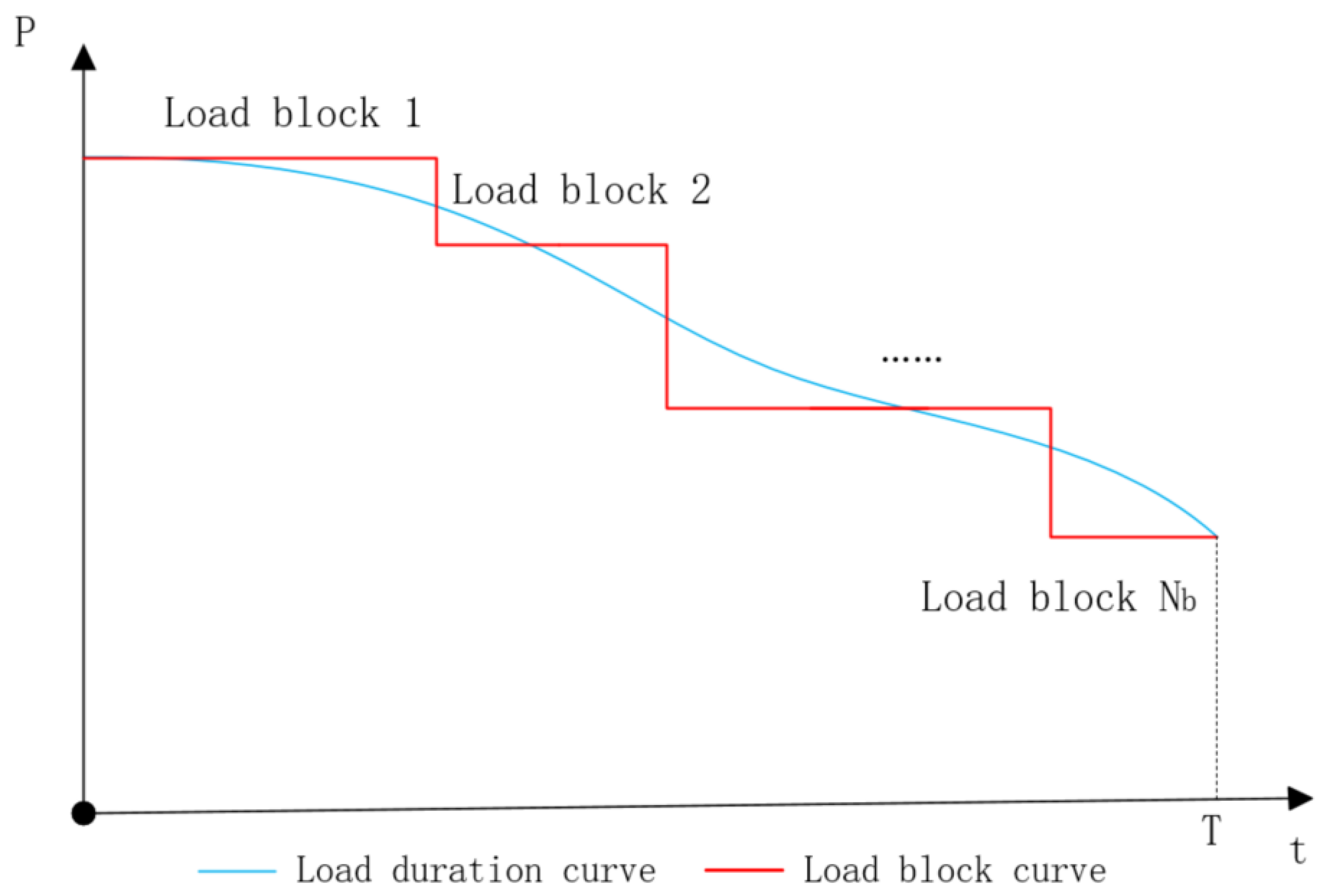
• According to the time series load curve, arrange the data in the load time series curve in descending order. Then, the accurate duration curve is obtained.
• Determine the number of load segments required for the model calculation and select the load level corresponding to each load segment to obtain an approximate load segment curve. It should be noted that the load block curve should reflect the maximum and minimum loads. Therefore, the number of load blocks is generally not less than three blocks.
• Appropriately adjust each load block to ensure the total power of approximate load block curve equals that of the original sequential load curve.

According to the obtained block curve, the variables are defined. The objective function and constraints are constructed, and then the mid/long-term optimization model is established.

2.2. Renewable Energy Power Model

As the proportion of renewable energy continues to increase, the new power system will present a high degree of uncertainty in the future. In order to ensure the safe and economical supply of electrical energy in the power system, it is important to establish renewable energy power models that describe the intermittent nature of renewable energy output. With the deepening of the understanding of the characteristics of renewable energy, the model is also gradually improved.

This paper discusses renewable energy power models at mid/long-term scales. Based on the load block curve of each week (monthly), combined with the time series output curve of renewable energy, the probability distribution of renewable energy output corresponding to each week (monthly) and each load block can be obtained, as shown in Figure 2. The model can reflect the seasonality of renewable energy output as well as describe the temporal correlation of renewable energy output and load level. Through cluster analysis, sampling and other methods [56], the renewable energy output probability model can be transformed into the discrete model shown in Figure 3 for practical calculation. p^α=0.95_r,t,b in Figure 3 represents the renewable energy output with a 95% guarantee rate under load block b at t hour, which can be determined by the probability density function in Figure 2 and the quantile of the statistics of renewable energy output in Figure 3.

Due to the strong randomness of the output of renewable energy, in order to maintain electric power and electric energy balance of the power system, the output of the controllable power units needs to be adjusted according to the real-time renewable energy output. The adjustment of controllable power units’ outputs is shown in Figure 2. Assuming that the predicted power of the renewable energy output is p_r,t,b, when actual renewable energy output is less than p_r,t,b, it is necessary to call the upload reserve of the power system, that is, increase the output of the controllable unit or reduce the output of the controllable unit.

Limited by the adjustment capacity of the power system, when the power system has insufficient upward reserve or downward reserve, as shown in the shaded part in Figure 2, it will not be able to cope with the random changes in the output of renewable energy. The former will lead to load loss, while the latter will lead to renewable energy curtailment. In view of the above situation, the concept of renewable energy absorption interval is introduced: p^min_r,t,b is introduced to represent the lower limit of the renewable energy power that can be absorbed, which corresponds to the maximum upload reserve provided by the system; p^max_r,t,b is used to represent the upper limit of the renewable energy power that can be absorbed, corresponding to the maximum value of the downward reserve. [p^min_r,t,b, p^max_r,t,b] is the renewable energy absorption interval. When the output power of the renewable energy falls within this interval, the electric power and electric energy balance of the power system can be maintained by adjusting the output of the controllable units.

3. Model Description

Based on the renewable energy power model established above, this paper establishes a mid/long-term optimization model. This model takes the week as the basic time unit to realize the complementarity of the power supply and loads on mid/long-term time scales and promote renewable energy absorption.

3.1. Objective Function

From Section 2, the renewable energy absorption interval is limited by the upload and download adjustment capability of the controllable energy units. The cross-regional power transmission channel can also provide upload and download reserve. Therefore, the change of renewable energy absorption interval should also take the cross-regional power trade into account. In other words, the power system operation is reflected in the renewable energy absorption interval, so it is meaningful to incorporate the renewable energy absorption interval into the objective function.

In addition to the fuel cost of the thermal power unit, the renewable energy curtailment penalty, and the loss of load penalty, the model also considers the penalty of renewable energy absorption interval. The objective function is expressed as follows:

$$\begin{array}{l}\min {\displaystyle {\displaystyle \sum }_{t=1}^{T_{\mathrm{total}}}}{\displaystyle {\displaystyle \sum }_{b=1}^{NU{M}_b}}[{\displaystyle {\displaystyle \sum }_g^{NU{M}_g}}{f}_g\left(p_{g,t,b}\right)+{\lambda }^{RC}R{C}_{t,b}+{\lambda }^{LC}L{C}_{t,b}\hfill \\ +{\lambda }^{pr\min }{\displaystyle {\displaystyle \sum }_r^{NU{M}_r}}{p}_{r,t,b}^{\min }+{\lambda }^{pr\max }{\displaystyle {\displaystyle \sum }_r^{NU{M}_r}}{p}_{r,t,b}^{\max }]D_{t,b}\hfill \end{array},$$

(1)

where T_total is the total number of time periods, NUM_b represents the load block number, g refers to thermal power unit label, r is the label of renewable energy power units, f_g(p_g,t,b) is the cost when the thermal power output is p_g,t,b, RC_t,b and LC_t,b respectively represent the cost of renewable energy curtailment and load loss, λ^RC and λ^LC respectively represent the cost of renewable energy curtailment and load loss, p^min_r,t,b and p^max_r,t,b are the lowest and highest power of the renewable energy absorption interval of the renewable energy power unit r, λ^prmin and λ^prmax respectively represent the penalty coefficient of the lowest and highest power of the renewable energy absorption interval and D_t,b is the duration.

3.2. Maintenance Constraints

The unit maintenance plan is a key part of the power system mid/long-term operation plan. It focuses on the economic principle of the power system and optimizes the dispatch of multiple types of energy in weeks (months) so as to optimize the power system production during the entire operation cycle. In the cross-regional interconnected power grid, reasonable unit maintenance plans can ensure the economy and safety of the power supply and also effectively cope with the differences in the structure, season and region of the interconnected power grids. Generally speaking, the maintenance constraints of units include maintenance time constraints, maintenance continuity constraints, maintenance duration constraints, maintenance interval time constraints and maintenance capacity constraints [57].

3.3. Unit Operation Constraints

This type of constraints [58] is mainly composed of constraints such as the start and stop constraints of the unit, the upper and lower limits of the unit output, and the capacity of the unit to provide upward and downward backup. In addition, according to the adjustment type of the hydropower unit, the water energy constraints of the hydropower plant need to be considered. The pumped storage power station maintains a balance of electricity as a whole, that is, the balance of pumped water energy and power generation energy. Considering the uncertainty of renewable energy output, the renewable energy absorption interval is used to represent the randomness of the renewable energy output.

This section will introduce the operating constraints of renewable energy units in detail below.

3.3.1. Renewable Energy Unit Power Output Constraints

This constraint represents the upper and lower limits of the power output of renewable energy units.

$$p_{r,t,b}^{\min }\le p_{r,t,b}\le p_{r,t,b}^{\max },$$

(2)

where p_r,t,b is the renewable energy unit r’ power.

3.3.2. Renewable Energy Expected Electric Energy Constraints

This constraint refers to the expected electricity generated from renewable energy units during the solution period.

$$R{E}_{t,b}={\displaystyle \sum }_s{\pi }_s{p}_{r,t,b}^s{D}_{t,b},$$

(3)

where RE_t,b represents the renewable energy expected electric energy, s represents the label of scenarios, π_s is the probability of the scenario s and p^s_r,t,b represents the power output of renewable energy unit r for scenario s.

3.3.3. Renewable Energy Curtailment Constraints

When the download reserve of the system is insufficient, the renewable energy curtailment occurs.

$$R{C}_{t,b}={\displaystyle \sum }{\pi }_s\max \left(0,p_{r,t,b}^s-p_{r,t,b}^{\max }\right)D_{t,b},$$

(4)

3.3.4. Load Loss Constraints

When the upload reserve is insufficient, the system loses load.

$$L{C}_{t,b}={\displaystyle \sum }_s{\pi }_s\max \left(0,p_{r,t,b}^{\min }-p_{r,t,b}^s\right)D_{t,b},$$

(5)

3.4. Cross-regional Power Trade Constraints

Cross-regional power trade can coordinate the problems of uneven distribution of resources and large cost differences between regions, and it is regarded as an optimal allocation scheme for power resources to simultaneously achieve economic, environmental and social benefits. Regarding the power transmission outside the tie line as the load of the sending-end power grid, with the actual operation of the tie line considered, this paper establishes a model of multiple cross-regional transmission channels to realize the coordination and optimization of renewable energy units, conventional units and tie lines in the sending-end power grid, which can adapt to the current grid dispatching mode. The following introduces cross-regional power trade in detail.

3.4.1. Cross-Regional Trade Power Constraints

The trade power of the tie line needs to meet the minimum trade power constraint and transmission capacity limits. In order to cope with the sudden increase or decrease of the power demand of the sending-end power grids and the receiving-end power grids, the tie line should also provide upload reserve and download reserve.

p_z,t,b − pdr_z,t,b ≥ p_z,min,

(6)

p_z,t,b − pur_z,t,b ≥ p_z,max,

(7)

0 ≤ pdr_z,t,b ≤ Δp_z,max,

(8)

0 ≤ pur_z,t,b ≤ Δp_z,max,

(9)

where z is the tie line label, p_z,min and p_z,max represent the lower and upper limit, pur_z,t,b is the upload reserve that the tie line z can provide, pdr_z,t,b is the download reserve that the tie line z can provide and Δp_z,max represents the power adjustable range of tie line z.

3.4.2. Cross-Regional Trade Energy Constraints

At present, cross-regional power trades are mainly mid/long-term power trades in actual operation, and mid/long-term power trades often stipulate the total electric energy traded.

$${\displaystyle {\displaystyle \sum }_{t=1}^{T_{\mathrm{total}}}}{\displaystyle {\displaystyle \sum }_{b=1}^{NU{M}_b}}{\displaystyle {\displaystyle \sum }_{z=1}^{NU{M}_z}}{p}_{z,t,b}{D}_{t,b}=Q_z,$$

(10)

where NUM_z represents the total number of tie lines and Q_zis the trade electric energy.

3.5. System Operation Constraints

In addition to the constraints for each unit, the power system also needs to meet constraints such as electric power balance, electric energy balance and system reserve capacity during operation to ensure the safe and stable operation of the system [59].

3.5.1. Electric Power Balance Constraints

This constraint means that the electrical power supply and consumption of the system are kept in real-time balance.

$${\displaystyle {\displaystyle \sum }_{g=1}^{NU{M}_g}}{p}_{g,t,b}+{\displaystyle {\displaystyle \sum }_{h=1}^{NU{M}_h}}{p}_{h,t,b}+{\displaystyle {\displaystyle \sum }_{r=1}^{NU{M}_T}}{p}_{r,t,b}+{\displaystyle {\displaystyle \sum }_{q=1}^{NU{M}_q}}\left(p{g}_{q,t,b}-p{p}_{q,t,b}\right)=L_{t,b}+{\displaystyle {\displaystyle \sum }_{z=1}^{NU{M}_z}}{p}_{z,t,b},$$

(11)

where p_h,t,b is the power output of hydropower unit h, pg_q,t,b is the generating power, pp_q,t,b is the pumping power and L_t,b is the load power.

3.5.2. Electric Energy Balance Constraints

This constraint means that the electric energy supply and consumption of the system maintain a real-time balance in a period of time.

$$\begin{array}{l}{\displaystyle {\displaystyle \sum }_{g=1}^{NU{M}_g}}{p}_{g,t,b}{D}_{t,b}+{\displaystyle {\displaystyle \sum }_{h=1}^{NU{M}_h}}{p}_{h,t,b}{D}_{t,b}+R{E}_{t,b}-R{C}_{t,b}+L{C}_{t,b}+{\displaystyle {\displaystyle \sum }_{q=1}^{NU{M}_q}}\left(p{g}_{q,t,b}-p{p}_{q,t,b}\right)D_{t,b}\hfill \\ =\left(L_{t,b}+{\displaystyle {\displaystyle \sum }_{z=1}^{NU{M}_z}}{p}_{z,t,b}\right)D_{t,b}\hfill \end{array},$$

(12)

3.5.3. System Reserve Constraints

The constraints include upload and download reserve constraints.

$${\displaystyle \sum }_{g}pu{r}_{g,t,b}+{\displaystyle \sum }_{h}pu{r}_{h,t,b}+{\displaystyle \sum }_{q}pu{r}_{q,t,b}+{\displaystyle \sum }_{z}pu{r}_{z,t,b}\ge p_{r,t,b}-p_{r,t,b}^{\min },$$

(13)

$${\displaystyle \sum }_{g}pd{r}_{g,t,b}+{\displaystyle \sum }_{h}pd{r}_{h,t,b}+{\displaystyle \sum }_{q}pd{r}_{q,t,b}+{\displaystyle \sum }_{z}pd{r}_{z,t,b}\ge p_{r,t,b}-p_{r,t,b}^{\min },$$

(14)

where pur_g,t,b, pur_h,t,b, pur_q,t,b are the upload reserves that the thermal power unit g, hydropower unit h and pumped water power unit p can provide; pdr_g,t,b, pdr_h,t,b, pdr_q,t,b refer to the download reserve that the thermal power unit g, hydropower unit h and pumped-storage power unit p can provide.

4. Case Studies

This paper takes the adapted IEEE-RTS1979 [60,61] as an example for case studies. The analysis period is 1 year (52 weeks), and the annual maximum power load is 2850 MW. The power system includes eight thermal power plants with 26 units and with the installed gross capacity of 3105 MW, one hydropower station with six units and with the installed gross capacity of 300 MW and one pumped-storage power station with four units and with the installed gross capacity of 200 MW. Each unit can be repaired once every year, lasting 3 to 4 weeks each time, and the number of units that can be repaired at the same time in each power plant is one. The renewable energy output data come from a renewable energy power plant in northwest China, including two renewable energy power units and with the installed gross capacity of 800 MW. The renewable energy curtailment penalty is 5 $/MWh, and the load loss penalty is 10,000 $/MWh. The annual cross-regional trade energy is 400,000 MWh, and the output power interval of the tie lines is [10 MW, 200 MW). Considering factors such as solution accuracy and calculation scale, the calculation example selects the load block curve divided into four blocks.

4.1. The Base Case

When the renewable energy absorption interval penalty and cross-regional power trade are not considered, the model established in this paper is solved according to the above calculation conditions to obtain the main production indicators of the power system shown in

Table 3. Operation indices.

Total Thermal Power Cost (107 $)	Per Thermal Power Cost ($/MWh)	Probability of Renewable Energy Spills (%)
6.3908	12.5369	5.6833

.

Based on the results of the base case, the following will address the impacts of cross-regional power trade and renewable energy grid integration on the operation of the power system and fully exploit the role of cross-regional power trade in promoting renewable energy consumption.

4.2. Analysis of the Influence of Quarterly Arrangements in Cross-Regional Power Trade

In the actual operation of the power system, due to the uneven distribution of power and load in each region of the interconnected grid, a reasonable cross-regional power trade plan can alleviate the contradiction between supply and demand. In the actual production scheduling, the sending-end power grid will comprehensively analyze its own power surplus and the power demand of the receiving-end power grid to arrange the surplus power delivery plan. When the local consumption of renewable energy cannot be satisfied, transferring local renewable energy through the tie line to adjacent areas with large load can effectively avoid renewable energy curtailment.

According to the quarterly arrangement of the cross-regional power trade, the following three scenarios will be considered: (1) Scenario 1: evenly distributed; (2) Scenario 2: considering load characteristics; (3) Scenario 3: considering load characteristics and renewable energy characteristics. By solving the model, the main production indicators of the system and the cross-regional weekly trade electricity plan are obtained, as shown in

Table 4. Operation indices.

Scenario	Total Thermal Power Cost (107 $)	Per Thermal Power Cost ($/MWh)	Probability of Renewable Energy Spills (%)
1	6.2551	12.6416	4.6579
2	6.2772	12.7028	4.5779
3	6.2488	12.6589	4.4791

and Figure 4.

From Table 3 and Table 4, it can be found that cross-regional power trade plays an effective role in promoting the coordination and optimization of conventional energy and renewable energy in the interconnected grids, and the total thermal power cost is lower than when cross-regional power trade is not considered. For areas with surplus renewable energy, cross-regional power trade can cope well with the volatility of renewable energy output and promote renewable energy consumption; it is shown that the probability of renewable energy spills drops in Table 4. It can be seen from the cross-regional power trade power in Figure 4 that, in the above three scenarios, Scenario 3 takes into account both the load change and the output change of renewable energy, and the sending-end grid sends more electricity when the output of renewable energy becomes large

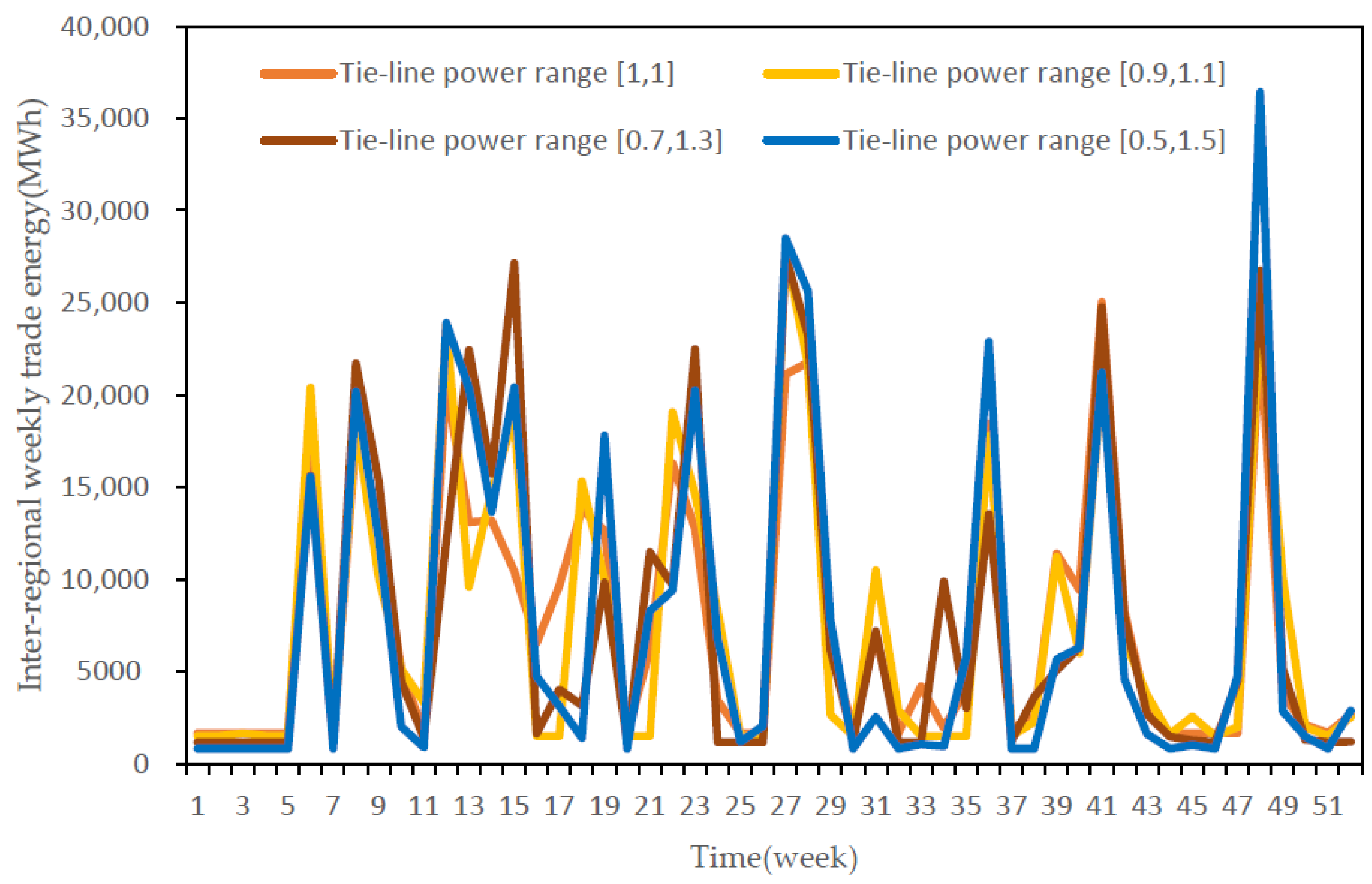
4.3. Analysis of the Influence of Tie-Line Power Range

For the receiving-end power grid, receiving power through the tie line during peak load times can relieve the electric power supply pressure. For the sending-end power grid, when the renewable energy output peaks, the electric power is sent out through the tie line, which can improve the renewable energy absorption capacity of the sending-end power grid. In the interconnected power grid with a high proportion of renewable energy access, making full use of the advantages of flexible control of the tie lines can tap the potential of the tie lines in promoting cross-regional renewable energy consumption, thereby promoting the load complementation and renewable energy acceptance between the sending-end power grid and the receiving-end power grid. On the basis of the discussion results in Section 4.2., it is assumed that the cross-regional trade electricity is quarterly distributed considering the load characteristics and renewable energy characteristics. The following will adjust the power range of the tie line to solve the system operating indicators, as shown in

Table 5. Operation indices.

Tie-Line Power Range	Total Thermal Power Cost (107$)	Per Thermal Power Cost ($/MWh)	Probability of Renewable Energy Spills (%)
[1, 1]	6.2488	12.6589	4.4791
[0.9, 1.1]	6.2571	12.6747	4.5031
[0.7, 1.3]	6.2271	12.5792	4.6441
[0.5, 1.5]	6.2384	12.7315	4.1430

, and the cross-regional weekly traded electricity, as shown in Figure 5.

It can be seen from Table 5 that with the increase of the power range of the tie line, the adjustment capacity of the tie line is enhanced, which effectively reduces the peak regulation pressure of conventional energy units, and the total cost of thermal power units in Table 5 decreases. When the power range of the tie line is [0.7, 1.3], the total cost of thermal power is the lowest among the four cases. At the same time, the increase in the power range of the tie line also means that the power system has an increase in available resources when dealing with the volatility of renewable energy sources. When the power range of the tie line is [0.5, 1.5], the probability of renewable energy spills is 4.1430%, reaching the lowest value among the four cases. Due to the strong seasonal characteristics of the power supply and load in the power system, appropriately increasing the power range of the tie line can flexibly respond to extreme situations of power supply and demand. It can be seen from Figure 5 that when the power range of the tie line increases, the cross-regional weekly trade energy will peak at certain times, which indicates that the power grid has more surplus energy that needs to be sent out at the time. Otherwise, it will cause a power outage. When the operating goals of the power system are focused, such as minimizing the total cost of thermal power or reducing the probability of renewable energy spills, the ideal operating state can be achieved by appropriately adjusting the power range of the tie line according to the goals.

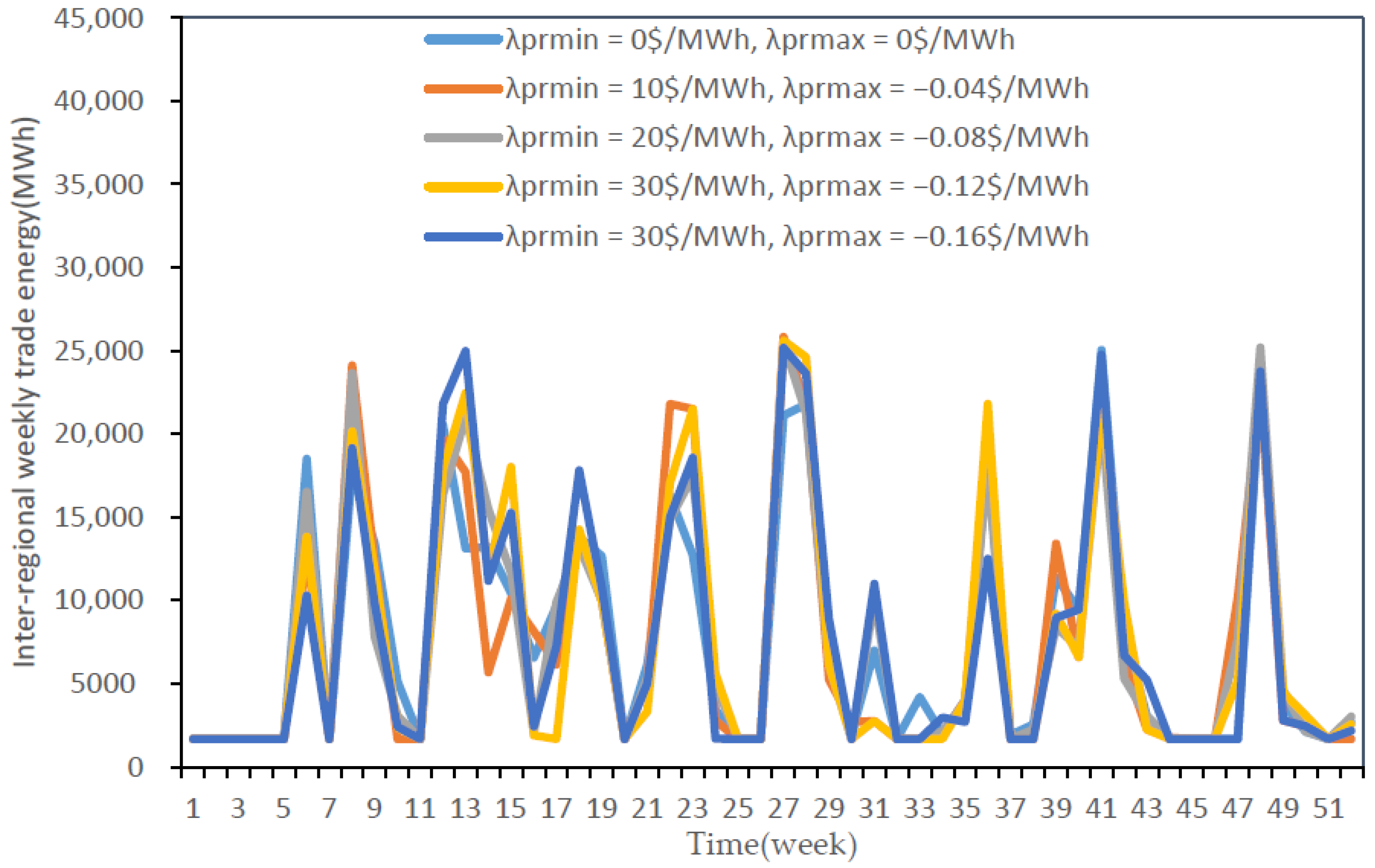
4.4. Analysis of the Influence of Renewable Energy Absorption Interval Penalty Coefficient

To give full play to the flexible adjustment ability of the tie line and reasonably arrange the power transaction plan between the interconnected power grids to relieve the pressure of peak regulation, one can reduce the conventional standby demand of the power grid, so as to effectively realize the coordination and optimization of the power supply and the load in the system. Considering the influence of cross-regional power trade on the consumption of renewable energy, the penalty of the renewable energy absorption interval is included in the objective function. The cross-regional power trade plans are adjusted on the basis of the change of the renewable energy absorption interval, so as to strengthen the link between changes in renewable energy output and interconnected grid electricity trading arrangements, to optimize the operation of the power system. The following assumes that the cross-regional trade energy is distributed quarterly, considering load characteristics and renewable energy characteristics, and the tie line’s power range is [10 MW, 200 MW]. The parameters of the renewable energy absorption interval cost will be adjusted to obtain the system operation indices shown in

Table 6. Operation indices.

Renewable Energy Absorption Interval Cost	Total Thermal Power Cost (107$)	Per Thermal Power Cost ($/MWh)	Probability of Renewable Energy Spills (%)
λprmin = 0 $/MWh λprmax = 0 $/MWh	6.2488	12.6589	4.4791
λprmin = 10 $/MWh λprmax = −0.04 $/MWh	6.2605	12.6816	4.5230
λprmin = 20 $/MWh λprmax = −0.08 $/MWh	6.2610	12.6919	4.4627
λprmin = 30 $/MWh λprmax = −0.12 $/MWh	6.2529	12.6824	4.4585
λprmin = 30 $/MWh λprmax = −0.16 $/MWh	6.2487	12.6700	4.4410

and the inter-region weekly transaction electric quantity shown in Figure 6.

From the data in Table 6, it is easy to find that the total cost of thermal power, per thermal power cost and the probability of renewable energy spills all decrease after considering the cost of renewable energy absorption interval. This shows that the consideration of renewable energy absorbing interval penalty can make full use of the many resources of the power system, optimize the allocation of conventional energy and renewable energy, and improve the regulating performance of the power system. As shown in Figure 6, after considering the range cost of renewable energy, the change of weekly trade energy becomes slow, which is more consistent with the actual operation of the power system, indicating the effectiveness of the model.

5. Conclusions

Renewable energy such as wind power generation and photovoltaic power generation has obvious seasonal characteristics, which brings new challenges in mid/long-term operation. Cross-regional power trade plays an essential role in ensuring the economic and safe operation of the power system when renewable energy is connected to the grids on a large scale. In this paper, considering the close relationship between the output range of renewable energy and the regulation resources in the system, the cross-regional power transmission channels are seen as flexible regulation resources. The mid/long-term optimization model takes maintenance constraints, unit operation constraints, cross-regional trade constraints and system operation constraints into account. On the basis of the results of the adapted IEEE-RTS, the influences of quarterly arrangement in cross-regional power trade, power range of tie lines, and renewable energy absorption interval penalty coefficient on the power system operation are analyzed. It is verified that the model can realize the reasonable planning of cross-regional power transactions. Therefore, renewable energy will be preferentially consumed.

References

1. Abdmouleh, Z.; Alammari, R.A.M.; Gastli, A. Review of policies encouraging renewable energy integration & best practices. Renew. Sustain. Energy Rev. 2015, 45, 249–262. [Google Scholar]
2. Hannele, H.; Peter, M.; Antje, O. Impacts of large amounts of wind power on design and operation of power systems, results of IEA collaboration. Wind Energy 2011, 14, 179–192. [Google Scholar]
3. Bouffard, F.; Galiana, F.D. Stochastic security for operations planning with significant wind power generation. IEEE Trans. Power Syst. 2008, 23, 306–316. [Google Scholar] [CrossRef]
4. Hu, B.; Lou, S.; Li, H.; Wu, Y.; Lu, S.; Huang, X. Spinning reserve demand estimation in power systems integrated with large-scale photovoltaic power plants. Autom. Electr. Power Syst. 2015, 39, 15–19. [Google Scholar]
5. Bu, S.Q.; Du, W.; Wang, H.F. Probabilistic analysis of small-signal stability of large-scale power systems as affected by penetration of wind generation. IEEE Trans. Power Syst. 2012, 27, 762–770. [Google Scholar] [CrossRef]
6. Gautam, D.; Goel, L.; Ayyanar, R. Control strategy to mitigate the impact of reduced inertia due to doubly fed induction generators on large power systems. IEEE Trans. Power Syst. 2011, 26, 214–224. [Google Scholar] [CrossRef]
7. Shah, R.; Mithulananthan, N.; Bansal, R.C. A review of key power system stability challenges for large-scale PV integration. Renew. Sustain. Energy Rev. 2015, 41, 1423–1436. [Google Scholar] [CrossRef]
8. Nichita, C.; Luca, D.; Dakyo, B. Large band simulation of the wind speed for real time wind turbine simulators. IEEE Power Eng. Rev. 2007, 22, 63. [Google Scholar] [CrossRef]
9. Miranda, M.S.; Dunn, R.W. Spatially correlated wind speed modeling for generation adequacy studies in the UK. In Proceedings of the 2007 IEEE Power Engineering Society General Meeting, Tampa, FL, USA, 24–28 June 2007; pp. 1–6. [Google Scholar]
10. Li, D.; Chen, C. Wind speed model for dynamic simulation of wind power generation system. Proc. CSEE 2005, 25, 41–44. [Google Scholar]
11. Zhang, H.; Yin, Y.; Shen, H. A wind speed time series modeling method based on probability measure transformation. Autom. Electr. Power Syst. 2013, 37, 7–10. [Google Scholar]
12. Philippopoulos, K.; Deligiorgi, D. Statistical simulation of wind speed in Athens, Greece based on Weibull and ARMA models. Int. J. Energy Environ. Econ. 2009, 3, 151–158. [Google Scholar]
13. Doquet, M. Use of a stochastic process to sample wind power curves in planning studies. In Proceedings of the 2007 IEEE Lausanne Power Tech, Lausanne, Switzerland, 1–5 July 2007; pp. 663–670. [Google Scholar]
14. Woods, M.J.; Russell, C.J.; Davy, R.J. Simulation of Wind Power at Several Locations Using a Measured Time-Series of Wind Speed. IEEE Trans. Power Syst. 2013, 28, 219–226. [Google Scholar] [CrossRef]
15. Bibby, B.; Skovgaard, I.; Sorensen, M. Diffusion-type models with given marginals and auto-correlation function. Bernoulli 2005, 11, 191–220. [Google Scholar]
16. Laslett, D.; Creagh, C.; Jennings, P. A simple hourly wind power simulation for the South-West region of Western Australia using MERRA data. Renew. Energy 2016, 96, 1003–1014. [Google Scholar] [CrossRef] [Green Version]
17. Zou, J.; Lai, X.; Wang, N. Time series model of stochastic wind power generation. Power Syst. Technol. 2014, 38, 2416–2421. [Google Scholar]
18. Chen, P.; Pedersen, T.; Bak-Jensen, B. ARIMA-Based time series model of stochastic wind power generation. IEEE Trans. Power Syst. 2010, 25, 667–676. [Google Scholar] [CrossRef] [Green Version]
19. Papaefthymiou, G.; Klockl, B. MCMC for wind power simulation. IEEE Trans. Energy Convers. 2008, 23, 234–240. [Google Scholar] [CrossRef] [Green Version]
20. Liu, C.; Lu, Z.; Huang, Y. A new method to simulate wind power time series of large time scale. Power Syst. Prot. Control. 2013, 41, 7–13. [Google Scholar]
21. Li, C.; Liu, C.; Huang, Y. Study on the modeling method of wind power time series based on fluctuation characteristics. Power Syst. Technol. 2015, 39, 208–214. [Google Scholar]
22. Denaxas, E.A.; Bandyopadhyay, R.; Patiño-Echeverri, D.; Pitsianis, N. SynTiSe: A modified multi-regime MCMC approach for generation of wind power synthetic time series. In Proceedings of the 2015 Annual IEEE Systems Conference (SysCon) Proceedings, Vancouver, BC, Canada, 13–16 April 2015; pp. 668–674. [Google Scholar]
23. Brokish, K.; Kirtley, J. Pitfalls of modeling wind power using Markov chains. In Proceedings of the 2009 IEEE/PES Power Systems Conference and Exposition, Seattle, WA, USA, 15–18 March 2009; pp. 1–6. [Google Scholar]
24. Yu, P.; Li, J.; Wen, J. A wind power time series modeling method based on its time domain characteristics. Proc. CSEE 2014, 34, 3715–3723. [Google Scholar]
25. Li, J.; Zhu, D. Combination of moment-matching, Cholesky and clustering methods to approximate discrete probability distribution of multiple wind farms. IET Renew. Power Gener. 2015, 10, 1450–1458. [Google Scholar] [CrossRef]
26. Lin, C.; Bie, Z.; Pan, C.; Liu, S. Fast cumulant method for probabilistic power flow considering the nonlinear relationship of wind power generation. IEEE Trans. Power Syst. 2020, 35, 2537–2548. [Google Scholar] [CrossRef]
27. Pan, C.; Wang, C.; Zhao, Z.; Wang, J.; Bie, Z. A Copula function based monte carlo simulation method of multi-variate wind speed and PV power spatio-temporal series. Energy Procedia 2019, 159, 213–218. [Google Scholar] [CrossRef]
28. Collares-Pereira, M.; Rabl, A. The average distribution of solar radiation-correlations between diffuse and hemispherical and between daily and hourly insolation values. Sol. Energy 1979, 22, 155–164. [Google Scholar] [CrossRef]
29. Zhang, S.; Tian, S. The institution of the hourly solar radiation model. Acta Energ. Sol. Sin. 1997, 18, 273–277. [Google Scholar]
30. Xu, Q.; Zang, H.; Bian, H. Establishment and feasibility researches of practical solar Radiation Model. Acta Energ. Sol. Sin. 2011, 32, 1180–1185. [Google Scholar]
31. Rahman, S.; Khallat, M.A.; Salameh, Z.M. Characterization of insolation data for use in photovoltaic system analysis models. Energy 1988, 13, 63–72. [Google Scholar] [CrossRef]
32. Karaki, S.H.; Chedid, R.B.; Ramadan, R. Probabilistic performance assessment of autonomous solar-wind energy conversion systems. IEEE Trans. Energy Convers. 1999, 14, 766–772. [Google Scholar] [CrossRef]
33. Peng, C.; Huang, Y.; Wu, Z. Building-integrated photovoltaics (BIPV) in architectural design in China. Energy Build. 2011, 43, 3592–3598. [Google Scholar] [CrossRef]
34. Tiwari, G.N.; Mishra, R.K.; Solanki, S.C. Photovoltaic modules and their applications: A review on thermal modelling. Appl. Energy 2011, 88, 2287–2304. [Google Scholar] [CrossRef]
35. Sulaiman, M.Y.; Oo, W.M.H.; Wahab, M.A. Application of beta distribution model to Malaysian sunshine data. Renew. Energy 1999, 18, 573–579. [Google Scholar] [CrossRef]
36. Klöckl, B.; Papaefthymiou, G. Multivariate time series models for studies on stochastic generators in power systems. Electr. Power Syst. Res. 2010, 80, 265–276. [Google Scholar] [CrossRef]
37. Huang, R.; Huang, T.; Gadh, R. Solar generation prediction using the ARMA model in a laboratory-level micro-grid. In Proceedings of the IEEE Third International Conference on Smart Grid Communications, Tainan, Taiwan, 5–8 November 2012; pp. 528–533. [Google Scholar]
38. Hassanzadeh, M.; Etezadi-Amoli, M.; Fadali, M.S. Practical approach for sub-hourly and hourly prediction of PV power output. In Proceedings of the North American Power Symposium, Arlington, TX, USA, 26–28 September 2010; pp. 1–5. [Google Scholar]
39. Ding, M.; Xu, N. A method to forecast short-term output power of photovoltaic generation system based on Markov Chain. Power Syst. Technol. 2011, 35, 152–157. [Google Scholar]
40. Li, R.; Li, G. Photovoltaic power generation output forecasting based on support vector machine regression technique. Electr. Power 2008, 41, 74–78. [Google Scholar]
41. Zhong, H.; Xia, Q.; Ding, M.; Zhang, H. A new mode of HVDC tie-line operation for maximizing renewable energy accommodation. Autom. Electr. Power Syst. 2015, 39, 6–42. [Google Scholar]
42. Xu, F.; Ding, Q.; Han, H.; Xie, L.; Lu, M. Power optimization and analysis of HVDC tie-line for promoting integration of cross-regional renewable energy accommodation. Autom. Electr. Power Syst. 2017, 41, 152–159. [Google Scholar]
43. Cheng, X.; Cheng, C.; Shen, J.; Li, G.; Lu, J. Coordination and optimization methods for large-scale trans-regional hydro-power transmission via UHVDC in regional and provincial power grids. Autom. Electr. Power Syst. 2015, 39, 151–158. [Google Scholar]
44. Ahmadi, A.; Conejo, A.J.; Cherkaoui, R. Multi-area energy and reserve dispatch under wind uncertainty and equipment failures. IEEE Trans. Power Syst. 2013, 28, 4373–4383. [Google Scholar] [CrossRef]
45. Ahmadi, A.; Conejo, A.J.; Cherkaoui, R. Multi-area unit scheduling and reserve allocation under wind power uncertainty. IEEE Trans. Power Systems. 2014, 29, 1701–1710. [Google Scholar] [CrossRef]
46. Frunt, J.; Kechroud, A.; Kling, W.L.; Myrzik, J.M.A. Participation of distributed generation in balance management. In Proceedings of the IEEE/PES Power Tech 2009, Bucharest, Romania, 28 June–2 July 2009; Piscataway: Institute of Electrical and Electronics Engineers: Bucharest, Romania, 2009; pp. 1–6. [Google Scholar]
47. Jiang, R.; Wang, J.; Guan, Y. Robust unit commitment with wind power and pumped storage hydro. IEEE Trans. Power Syst. 2012, 27, 800–810. [Google Scholar] [CrossRef]
48. Xu, Q.; Deng, C.; Zhao, W. A multi-scenario robust dispatch method for power grid integrated with wind farms. Power Syst. Technol. 2014, 38, 653–661. [Google Scholar]
49. Wu, W.; Chen, J.; Zhang, B. A robust wind power optimization method for look-ahead power dispatch. IEEE Trans. Sustain. Energy 2014, 5, 507–515. [Google Scholar] [CrossRef]
50. Chen, J.; Wu, W.; Zhang, B. A robust interval wind power dispatch method considering the tradeoff between security and economy. Proc. CSEE 2014, 34, 1033–1040. [Google Scholar]
51. Li, Z.; Wu, W.; Zhang, B. A robust interval economic dispatch method accommodating large-scale wind power generation part one dispatch scheme and mathematical model. Autom. Electr. Power Syst. 2014, 38, 33–39. [Google Scholar]
52. Sial, A.; Singh, A.; Mahanti, A. Detecting anomalous energy consumption using contextual analysis of smart meter data. Wirel. Netw. 2021, 27, 4275–4292. [Google Scholar] [CrossRef]
53. Sial, A.; Singh, A.; Mahanti, A.; Gong, M. Heuristics-Based detection of abnormal energy consumption. In Lecture Notes of the Institute for Computer Sciences, Social Informatics and Telecommunications Engineering; Chong, P., Seet, B.C., Chai, M., Rehman, S., Eds.; Smart Grid and Innovative Frontiers in Telecommunications; Smart GIFT 2018; Springer: Cham, Switzerland, 2018; Volume 245. [Google Scholar]
54. Sial, A.; Jain, A.; Singh, A.; Mahanti, A. Profiling energy consumption in a residential campus. In Proceedings of the 2014 CoNEXT on Student Workshop (CoNEXT Student Workshop’14), Sydney, Australia, 2 December 2014; Association for Computing Machinery: New York, NY, USA, 2014; pp. 15–17. [Google Scholar]
55. Shao, C.; Wang, Y.; Feng, C.; Wang, X.; Wang, B. Mid/long-term power system production simulation considering multi-energy generation. Proc. CSEE 2020, 40, 4072–4081. [Google Scholar]
56. Xu, J.; Yi, X.K.; Sun, Y.Z. Stochastic optimal scheduling based on scenario analysis for wind farms. IEEE Trans. Sustain. Energy. 2017, 8, 1548–1559. [Google Scholar] [CrossRef]
57. Feng, C.Y.; Wang, X.F. Review of generator maintenance scheduling in power market. Autom. Electr. Power Syst. 2007, 31, 97–104. [Google Scholar]
58. Wang, Y.; Shao, C.; Sun, P.; Wang, X.; Wang, X.; Li, D. Generator maintenance schedule considering characteristics of multi-type renewable energy. In Proceedings of the 2018 International Conference on Power System Technology (POWERCON), Guangzhou, China, 6–8 November 2018; pp. 4050–4055. [Google Scholar]
59. Ma, X.; Zhang, Z.; Bai, B.; Ren, X.; Kang, K. Mid/long-term power system operation model considering inter-regional power trade. In Proceedings of the 2021 IEEE 2nd China International Youth Conference on Electrical Engineering (CIYCEE), Chengdu, China, 15–17 December 2021; pp. 1–6. [Google Scholar]
60. Probability Methods Subcommittee. IEEE reliability test system. IEEE Trans. Power Appar. Syst. 1979, 98, 2047–2054. [Google Scholar]
61. Wang, S.J.; Shahidehpour, S.M.; Kirschen, D.S.; Mokhtari, S.; Irisarri, G.D. Short-term generation scheduling with transmission and environmental constraints using an augmented Lagrangian relaxation. IEEE Trans. Power Syst. 1995, 10, 1294–1301. [Google Scholar] [CrossRef]
Figure 1. Load duration curve and load block curve.
Energies 15 03594 g001
Figure 2. Renewable energy output probability model.
Energies 15 03594 g002
Figure 3. Renewable energy output discrete model.
Energies 15 03594 g003
Figure 4. Cross-regional weekly trade energy.
Energies 15 03594 g004
Figure 5. Cross-regional weekly trade energy.
Energies 15 03594 g005
Figure 6. Cross-regional weekly trade energy.
Energies 15 03594 g006