Impact of the COVID-19 Pandemic Crisis on the Efficiency of European Intraday Electricity Markets

Abstract

Our goal is to examine the efficiency of different intraday electricity markets and if any of their price prediction models are more accurate than others. This paper includes a comprehensive review of Germany, France, and Norway’s (NOR1) day-ahead and intraday electricity market prices. These markets represent different energy mixes which would allow us to analyze the impact of the energy mix on the efficiencies of these markets. To draw conclusions about extreme market conditions, (i) we reviewed the market data linked to COVID-19. We expected higher volatility in the lockdowns than before and therefore decrease in the efficiency of the prediction models. With our analysis, (ii) we want to draw conclusions as to whether a mix based mainly on renewable energies such as that in Norway implies lower volatilities even in times of crisis. This would answer (iii) whether a market with an energy mix like Norway is more efficient in highly volatile phases. For the analysis, we use data visualization and statistical models as well as sample and out-of-sample data. Our finding was that while the different price and volatility levels occurred, the direction of the market was similar. We could find evidence that our expectations (i–iii) were met.

1. Introduction

While digitalization and climate change continue, renewable electricity generation, such as wind and solar power, will be further expanded [1,2,3]. At the same time, SARS-CoV-2 (COVID-19) has a major impact on the entire global economy. Changes are particularly noticeable in the energy sector, as both supply and demand are affected. These effects were striking regarding WTI and BRENT oil prices, which in some cases fell into negative values in April 2020 [4]. Since the focus of this paper will be Europe, here are a few examples of European energy prices: The BRENT oil price dropped by 59% compared to its last peak on the 17th of February. Also, gas prices dropped to their lowest since 1995 at the same time [5]. Since the COVID-19 crisis had a major impact on other commodities, such as oil and gas, the question now arises as to the situation in the whole-sale electricity markets. Unlike other commodities, electricity cannot be stored to the same extent, which is why there are special features regarding price forecasts [6]. In contrast to the markets described, the electricity markets have a lower market extent of liquidity, leading to a wider bid-ask spread [7]. The motivation of this paper is to analyze and compare different European short-term electricity markets by applying statistics to corresponding market data. We want to draw conclusions about the impact of the energy mix on prices and volatilities during periods of extreme market conditions caused by the effects of the COVID-19 pandemic crisis on the short-term electricity markets. The motivation is also to analyze if the extreme market conditions had an immediate impact on energy efficiency. Three markets were selected because each market represents a different main energy source. In other words, this research aims to point out the impact on a market relying mainly on wind energy and lignite (Germany), a market relying on nuclear power (France), and a market relying on hydropower (Norway) [8].

Like what has already been done with other commodities, one aim of this paper is to divide the period of 01.01.2020 to 01.02.2021 into different phases and highlight the impacts of the lockdowns. The paper by J. Ali and W. Kahn (2020) serves as a model for this procedure. They looked at the agricultural commodity prices for various products in India and examined the influences on prices in the individual phases of the local lockdowns. They found that the weighted average of prices fell during the lockdown [9]. Some papers focus on the links between the financial and commodity markets. One example is the paper of A. Elsayed et al. (2020). They investigate co-movements between the energy market and the financial markets. Furthermore, they analyze time patterns of volatility spillovers [10]. The research of Bompard et al. (2020) focuses on the immediate impact of COVID-19 on European Electricity systems. This paper considers the quantified impact of strategic decisions on regulation and system operations during the lockdown periods [11].

The paper by O. B. Adekoya and J. A. Oliyide (2021) highlights the link between financial and commodity markets. In addition, it refers to the main price drivers. These linkages are mainly captured by analyzing price movements and volatilities [12]. Our paper aims to analyze price and volatility movements as well. Among all financial assets, spot electricity prices belong to the most volatile asset classes. One of the reasons for the high volatility is the non-storable nature of volatility. In their study L. Han et al. point out the risks for the market participants caused by volatilities and extreme price outcomes. For their analysis, they also looked at the different market regions in Australia individually and then compared them with each other. We take a similar strategic approach in this paper, as we examine and compare various European markets based on their volatilities and prices [13]. In our paper, we aim to determine whether there is a link between the type of energy generation and the price or volatility movement in an extreme economic situation. In doing so, we will follow the approach of S. Halbrügge et al. (2021) and their comprehensive analysis of the German electricity market, as well as C. Fezzi and V. Fanghella (2020), who analyzed the Italian Electricity market [4,14]. In addition, Kuppelwieser and Wozabal (2021) followed a similar approach as it is done in this kind of research. They also made use of intraday power data considering out-of-sample data sets. In contrast to our research, they consider weather forecasting and algorithmic trading. Furthermore, they also took order data and market liquidity into account [7].

In the course of their research, C. Kath and F. Ziel (2018, 2021) examined the forecast accuracy by applying modern regression techniques [15] and conformal predictions [16] in short-term electricity markets [15,16]. The focus and novelty of our paper are not to create a forecast. Rather, we have applied statistics and visualization techniques to test the predictive accuracy in the volatile market. B. Finnah et al. used different approaches to visualizing short-term electricity data in combination with a statistical model. Their focus was on the German day-ahead and the intraday auction electricity markets [17]. K. Maciejowska et al. (2019) performed a region-based comparison between German and Polish short-term electricity data. They also made use of visualizations comparing the different datasets [18]. Kramer and Kiesel (2021) focused on a data visualization regarding the buy and sell order data for German short-term electricity markets (Figure 1). In their paper, they also pointed out how the day-ahead and intraday markets are structured. This graph also supports the understanding of our research [19]. Other factors that can influence electricity prices are extreme weather and bidding behavior. Ghosh et al. (2021) investigated the freeze in Texas in February 2021 and analyzed the effects of extreme weather conditions on electricity prices [20]. Xiao et al. (2021) conducted an analysis of the bidding behavior using virtual bidding. They focused on wind power producers in the course of their research [21].

To use (i) out-of-sample data to improve forecasting accuracy, which is defined as the price difference between intraday and day-ahead markets in a similar way to traditional asset management, we have examined two types of prices in extreme situations for this paper [16,22]. We used intraday prices as well as day-ahead prices. One of our goals is to determine whether the forecasting methods have been improved by using this data. The periods of March to May 2020 and December to February 2020/21 are crucial. In addition, countries in Europe reacted with different measures to the pandemic. Considering the COVID-19 measures and the (ii) different energy mixes, it leads to the question if it had an impact on the prices [13,23,24,25]. In other words, did the energy mix influence the prices during high volatility periods caused by lockdowns? To investigate the question, we looked at the energy markets in Germany, France, and Norway (NO1). Our overall research problem is whether (iii) the forecasting accuracy in the German intraday market has improved in the second lockdown.

1.1. Contributions

Following the guidelines presented in our research design (see Figure 2), we apply a rigorous, transparent, and reproducible methodology for our models and visualizations. All four types of figures follow the same coding methodology using different datasets. We will provide our readers with further details on our scripts when contacting the corresponding author. We are transparent about our data sources and codes being used regarding Bloomberg. We present how different energy mixes react to extreme market conditions in terms of market efficiency by applying our model to three different short-term electricity markets.

1.2. Paper Structure

The paper is structured as follows: we first present common methods regarding volatility and explain our calculation method with regard to confidence intervals. After that, we looked at the data we used. Our results are structured as follows: A general introduction to our approach, followed by a structured analysis looking first at intraday and then at day-ahead prices. In the case of Germany and France, we have also analyzed the volumes. This is followed by a discussion, conclusion, and outlook. To present our results, we refer to (i) extreme market conditions, (ii) the energy mix, and (iii) energy efficiency.

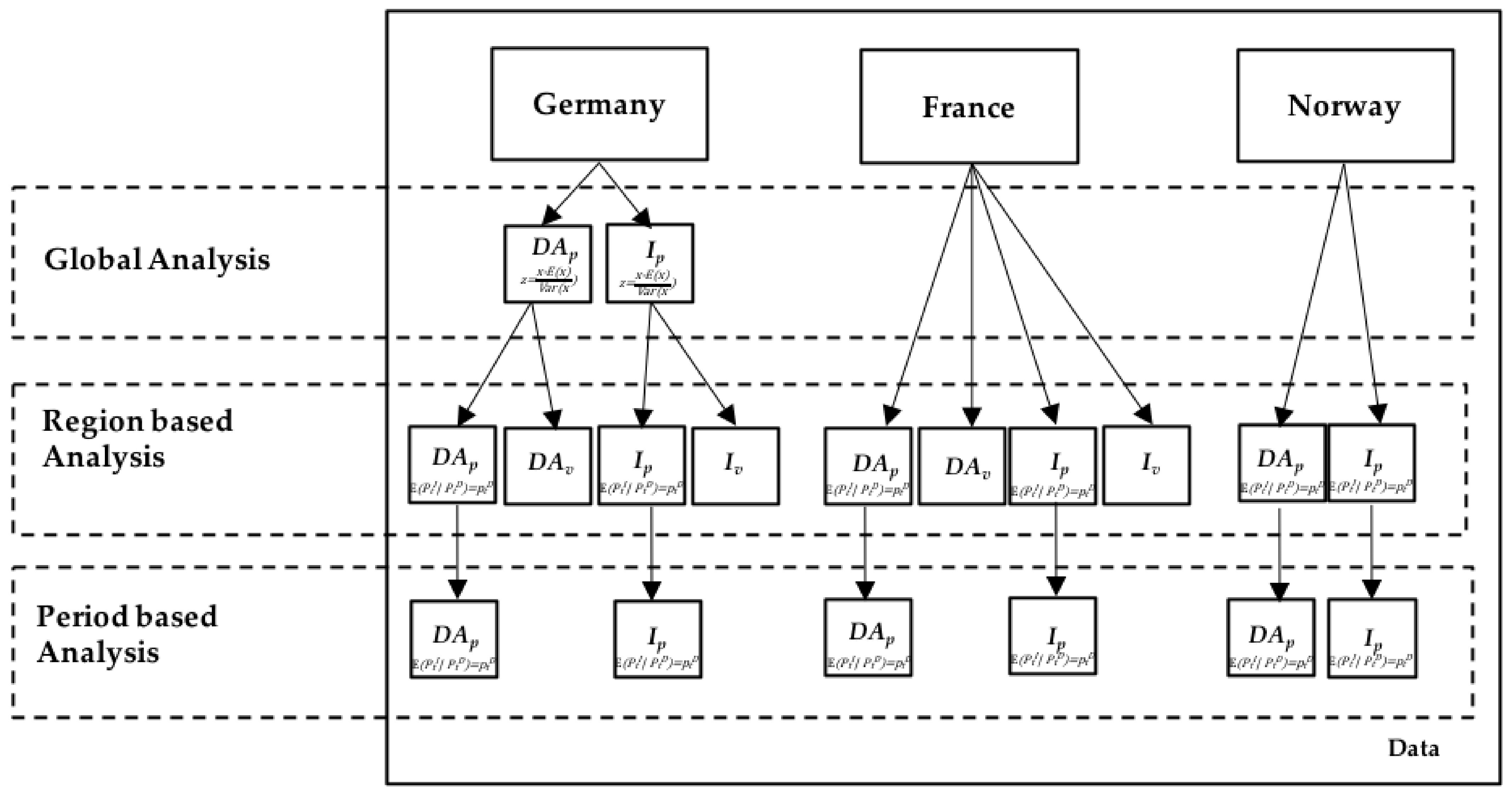
2. Materials and Methods

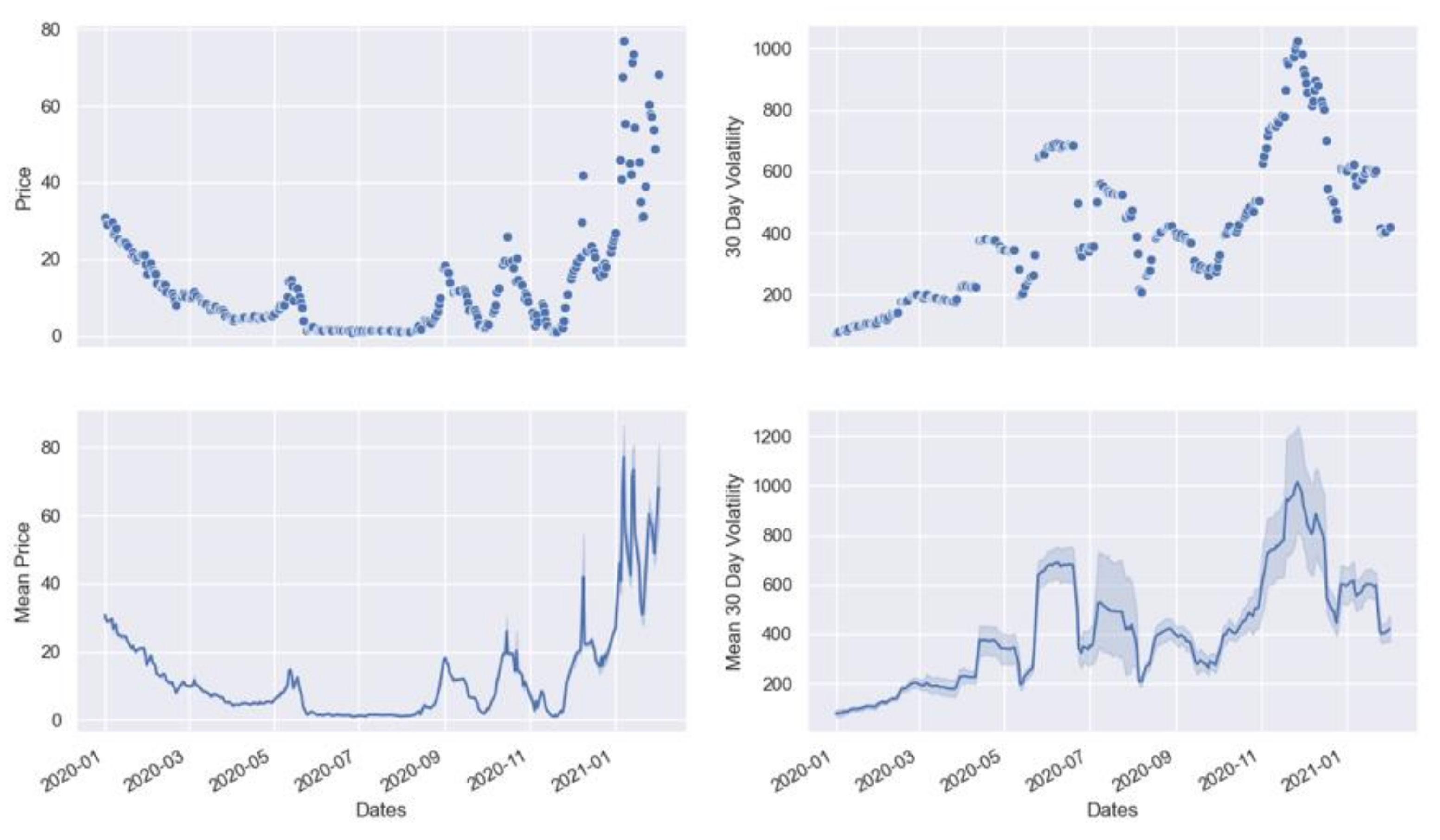
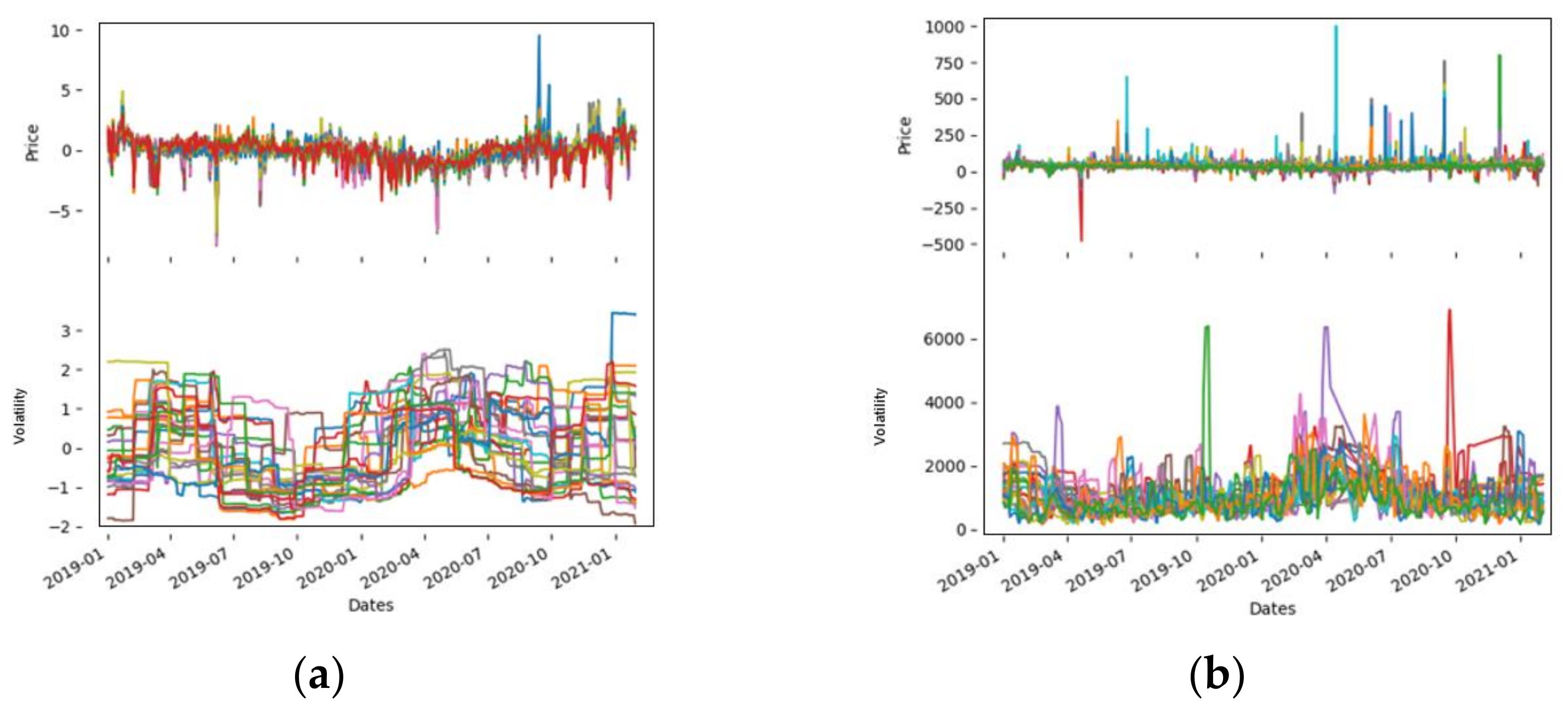
2.1. Price Analysis

We present the data and the corresponding statistical results using various visualization methods to draw a conclusion about the forecast accuracy in a volatile market, following an order that starts with a general overview via graphs. These graphs include all price data for German intraday and day-ahead electricity products. Afterwards, we divided the data into the observed regions (Germany, France, and Oslo—Norway) and added the 30-day volatility and confidence intervals to the analysis. The confidence intervals present the uncertainty estimates regarding the analyzed data. In addition, electricity generation was also taken into consideration. Thereby, we pointed out different energy sources (renewables and fossil fuels). The following statistical values are determined: Mean, median, standard deviation, and a 95% confidence interval. To calculate volatility, the following formula is used in literature for spot prices observed from historical data. Price returns are used in this example to obtain the volatility estimates [26].

$${\sigma }^{2}dt=E\left[{\left(\widetilde{dS/S}\right)}^2\right]$$

(1)

where:

• S = Spot Price
• σ = Spot Price Volatility
• dt = variance

Regarding the volatility figures, we made use of the 30- and 90-day volatility. Thereby, we retrieved the corresponding data from Bloomberg using the following codes: VOLATILITY_30D and VOLATILITY_90D.

To calculate the 95% confidence interval, which will be used in the visualizations, α is set to 0.05 using the standard normal approximation [27].

$${\beta }_k=\left[b_k-1.96se\left(b_k\right),b_k+1.96se\left(b_k\right)\right]$$

(2)

This type of analysis is carried out to draw connections between the lockdown periods, the price development, and the energy production. The focus is on the German market. The data for France and Norway (NO1) serves as support, as both countries/regions have different energy mixes.

$$z=\frac{x-E\left(x\right)}{Var\left(x\right)}$$

(3)

To perform the standardization according to the z-transformation, Formula (3) was applied. The standardization was carried out for the energy mixes and partly for German electricity prices [27].

$$\mathbb{E}\left(P_t^I| P_t^D\right)=p_t^D for t=1,2$$

(4)

Formula (4) represents the underlying message of the research. It states that the expected price of the intraday price is the day-ahead price. Our research incorporates this statement through the visual comparisons and continues to refer to it in the Results and Conclusion. In doing so, we want to highlight the extent to which the forecasts made were accurate in the tense market environment [28].

2.2. Volume Analysis

A volume analysis is included for Germany to prove that the price developments during the lockdown periods had the COVID-19 pandemic crisis as the main driver. For France, the volume data are used to support hypotheses. For NO1, this analysis is not performed as no data are available in Bloomberg. Similar to prices, the following statistical quantities are determined for German and French intraday and day-ahead volumes: Mean, Median, and Standard Deviation. For the German intraday and day-ahead volumes, an additional graph was created that also includes the 95% confidence interval. However, this type of analysis only serves to support the statements, whereby the focus is on the German spot market for electricity.

2.3. Programming Language

To run our calculations and create the visualizations, we used the programming language python. We used the packages pandas and scripy stats for the statistics and matplotlib and seaborn for our statistical graphics. For the standardization applied to some of the figures, we employed the standardscaler. This package removes the mean and scales of each variable to unit variance. The underlying mathematical approach is made transparent in Formula (3). The style used to set the colors of the graphs is the “darkgrid” style. We made use of visual studio code to create the graphs and calculate the statistics.

2.4. Data

2.4.1. Electricity Prices

For the price analysis, Bloomberg data for the German, French, and Norway (NO1) day-ahead and intraday prices have been used. As stated before, the 30-day-volatility and 90-day-volatility were retrieved from Bloomberg. The confidence intervals are based on their own calculations in Python. In the case of the German and French electricity prices, EPEX Spot prices were used. In the case of the Norwegian price data, prices from Nord Pool were used. All calculations are based on hourly data and their mean values. The prices for Germany, France, and NO1 prices were provided in euros. The analysis is based on the daily closing prices of the traded hours. In addition to the prices, the 30- and 90-day volatility was also subtracted for the same data set.

Table 1. General Statistics across all Price Categories in MWh/EUR.

Statistics	German Intraday	German Day-Ahead	France Intraday	France Day-Ahead	NO1 Intraday	NO1 Day-Ahead
count	6356	6532	5367	6532	6532	6248
mean	38.23	34.67	37.49	36.16	14.17	12.72
std	35.93	17.02	18.54	16.97	17.65	14.82
median	35.00	33.58	36.50	35.40	8.84	8.08
min	−150.00	−83.94	−25.20	−8.65	−1.73	0.02
max	1000.00	189.25	328.20	189.25	205.68	152.25

gives an overview of all relevant statistical data regarding the prices used. More than 5000 data points were used in each case.

The lockdown periods (

Table 2. Data for the statistical evaluation on electricity prices.

Observation Period	German Intraday	German Day -Ahead	France Intraday	France Day-Ahead	NO1 Intraday	NO1 Day-Ahead
January 2020	1 January 2020–31 January 2020	1 January 2020–31 January 2020	1 January 2020–31 January 2020	1 January 2020–31 January 2020	1 January 2020–31 January 2020	1 January 2020–31 January 2020
January 2021	1 January 2021–31 January 2021	1 January 2021–31 January 2021	1 January 2021–31 January 2021	1 January 2021–31 January 2021	1 January 2021–31 January 2021	1 January 2021–31 January 2021
First Lockdown	3 March 2020-4 May 2020	3 March 2020-4 May 2020	3 March 2020-4 May 2020	3 March 2020-4 May 2020	2 March 2020-1 April 2020	2 March 2020-1 April 2020
Second Lockdown	2 November 2020-1 February 2021	2 November 2020-1 February 2021	15 October 2020-15 December 2020	15 October 2020-15 December 2020	2 November 2020-1 February 2021	2 November 2020-1 February 2021
Summer Months	4 May 2020-30 September 2020	4 May 2020-30 September 2020	1 July 2020-30 September 2020	1 July 2020-30 September 2020	4 May 2020-30 September 2020	4 May 2020-30 September 2020

) may differ. On the one hand, the time series of data extends to 1 February 2021. On the other hand, various measures or news items have ushered in a period of higher volatility in the markets. Table 2 represents the data periods that have been used for the statistical calculations.

2.4.2. Electricity Volumes

For the volume analysis, the daily closing volume of the individual hours was used for further analysis. The same data set was also used regarding German and French volumes (

Table 3. General Statistics across German and French Volumes in MWh/EUR.

Statistics	German Intraday	German Day-Ahead	France Intraday	France Day-Ahead
count	5689	6816	6392	6486
mean	5689.82	24,379.26	169.43	14,082.17
std	2844.92	4164.75	288.43	2814.81
median	5805.00	23,881.50	40.00	13,963.10
min	0.00	14,441.00	0.00	6892.00
max	61,234.00	43,600.00	2917.00	25,013.00

).

The entire record refers to five business days in a week and does not include weekends and national bank holidays. If there was no data for a specific product in the record due to a bank holiday or if the product was not traded on that day due to low liquidity, the record will have a blank field.

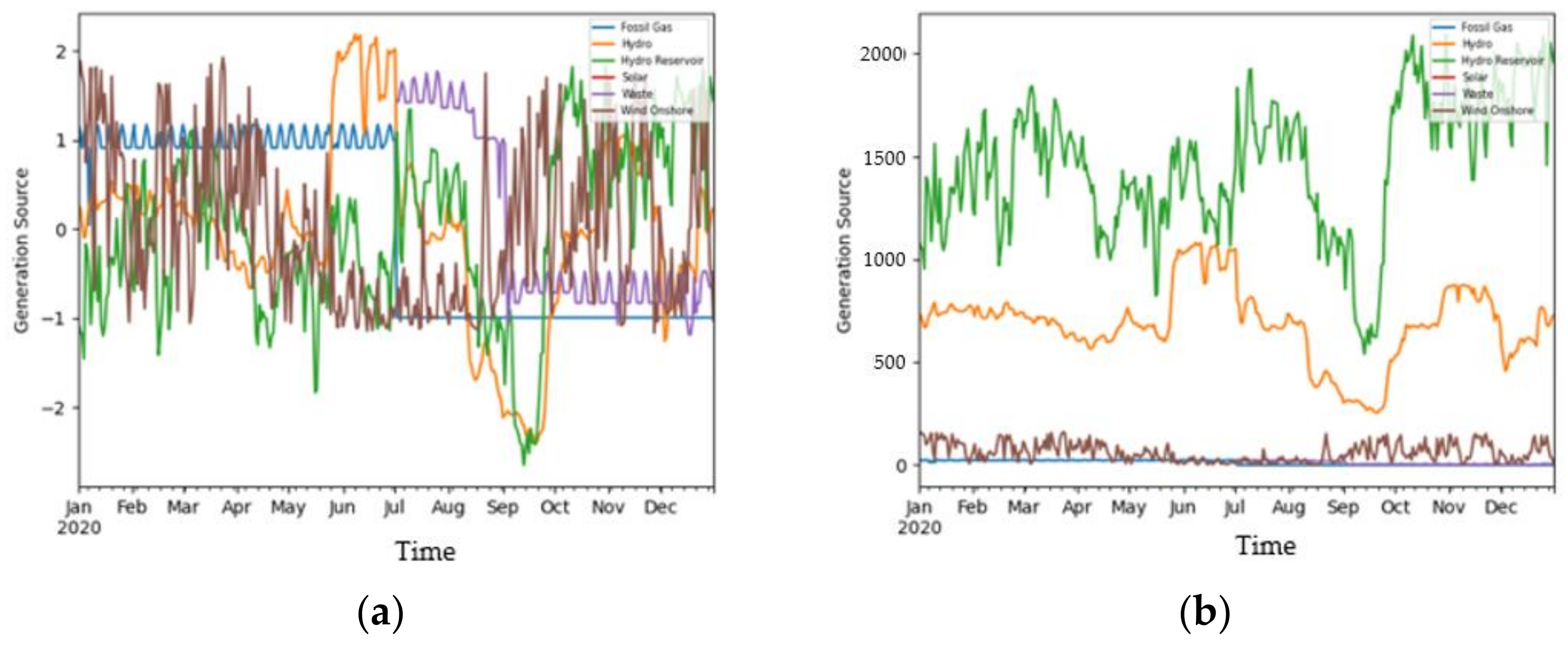
2.4.3. Electricity Generation

The electricity generation data was gathered from the ENTSO-E Transparency Platform. The observation period starts on 1 January 2020 and ends on 31 December 2020. To get a quick overview of the main electricity sources, we have plotted the main electricity generation sources per country. Figure 3, Figure 4 and Figure 5 show the standardized values on the left side and the non-standardized values in MWh on the right side [8].

3. Results

3.1. Results on the Overall Investigation

We translated our statistical results into graphs which enabled us to draw conclusions about the energy price and volatility situation during and between the two lockdowns in the three countries. Our summary statistics are presented in Table 1. We looked at intraday prices and day-ahead prices. The data is divided into a country/region-based analysis and two different lockdown periods. In addition, the 30-day volatility and the confidence intervals are considered as well. The following data is not standardized. The focus of the analysis will also be on the influence and crisis-proofing of renewable energies. Therefore, the electricity price development in France and the NO1 region in Oslo, Norway, will also be considered. For all three countries/regions, the following periods were considered: Price and volatility level in January 2020 as the pre-COVID-19 phase compared to the price level in January 2021. The respective first and second lockdown periods. The periods differ due to national regulations. In addition, the summer months are considered because the scope of the measures was small in all three countries.

The observation period from January 2019 to February 2021 was considered. The graph also takes into consideration the 90-day-volatility. One weakness of these graphs is that the overview is not always given (see Figure 6).

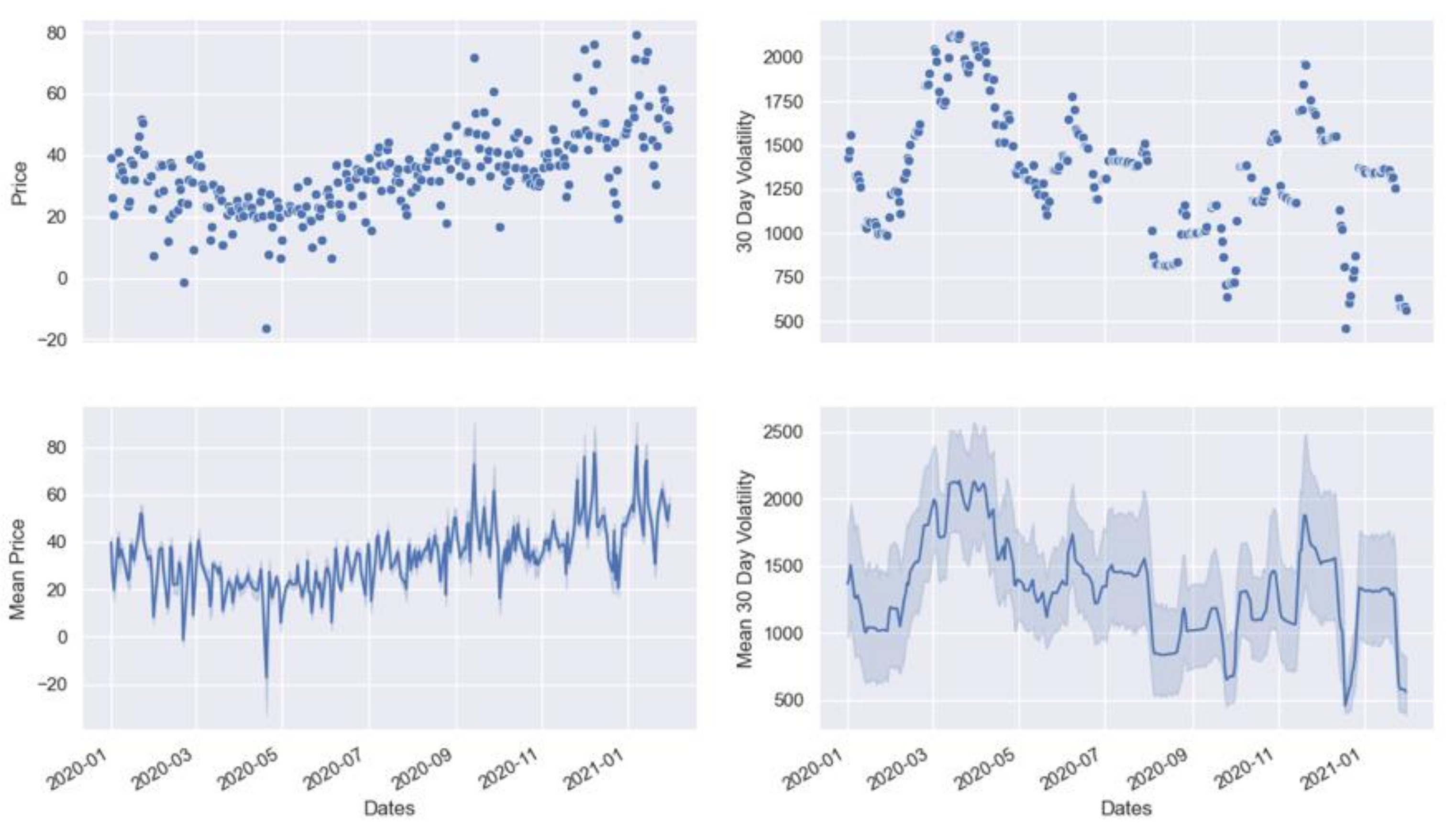
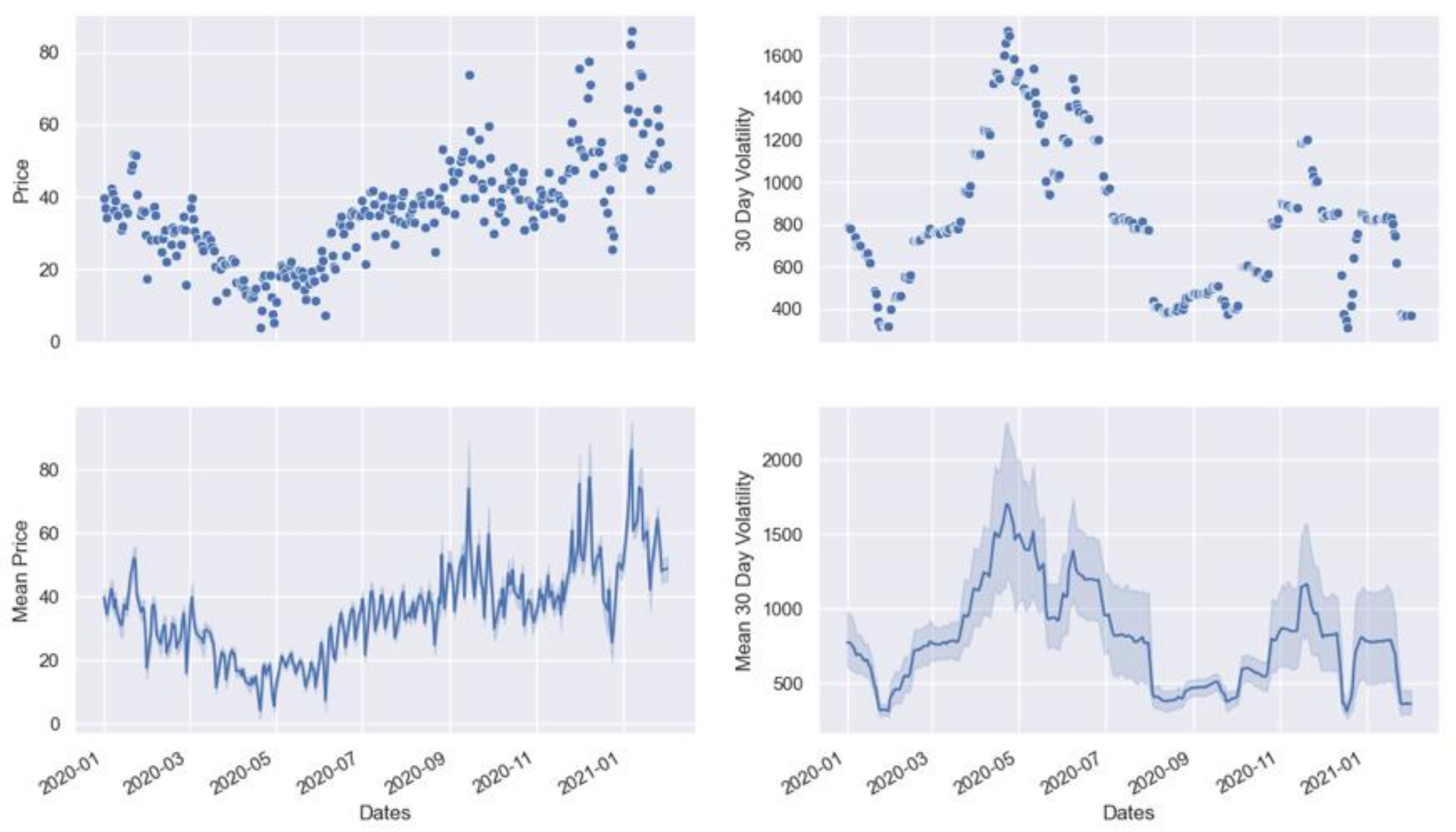
3.2. German Electricity Prices

In this part of the analysis, the German market is considered first. The graphs for French and Norwegian short-term power follow the same structure. On the left, there is always a presentation of the price level. The right sight displays the volatility development. The last two graphs include the mean as well as a 95% confidence level. A wide confidence level indicates more dispersion and, thus an uncertainty around the actual mean value. Germany had two lockdown periods during the observation period. The first lockdown period started in March 2020 and ended in May 2020. The second lockdown period started as a so-called soft lockdown in November and was then tightened in December. At the time of the data withdrawal in February 2021, the second lockdown in Germany had not yet ended [29]. In terms of the energy mix, Germany drew most of its energy from onshore wind power when it comes to the mean value analysis. Following the same mean value, approach lignite came in second place. It is striking with regard to the energy mix that none of the electricity generation sources make up the majority, i.e., have a share of over 50% [8].

3.2.1. German Intraday Prices

Figure 7 shows a clear increase in volatility in April 2020. The confidence level also shows greater volatility between April and May. In the second lockdown, volatility does not increase as much again. The reasons for the volatility increase in April 2020 could be many and varied. On the one hand, it could be related to the drop in oil prices, as there are correlations, or to weather data. This is particularly evident regarding the 30-day volatility, where a rise is visible after approximately fourteen days. However, this paper considers only the analysis of price, volatility, and production data. Correlations with other commodities are omitted [4,13]. Before April 2020, both prices and volatilities were at a stable level. After showing high outliers in April 2020, the price level recovered again. Therefore, in May, it was back at the level before April. The sample regarding the second lockdown starts on the first of November 2020 and ends on the first of February 2020 and indicates any similarities to the first lockdown. In contrast to the first lockdown, the price level remained at a higher level. Volatility, on the other hand, was lower. It recovered in May 2020, after the first lockdown, and remained at a constantly low level. Except for the numerous outliers highlighted in the price range based on confidence levels, the price movement shows an upward trend. For example, the price in January 2020 at 37.81 EUR is below the price in January 2021 at 54.51 EUR. The lowest price in the data set here is −150.00 EUR, and the highest price is 1000.00 EUR.

3.2.2. German Day-Ahead Prices

Figure 8 shows that the impact on volatility was greater on the day-ahead market than on the intraday market. Volatility shows the highest level during the first lockdown and decreases towards the end of the lockdown (

Table 4. General Statistics about German Prices and Volatilities in EUR.

Observation Period	Germany Intraday (Mean Price; Mean Vola)	Germany Intraday (Std Price; Std Vola)	Germany Day-Ahead (Mean Price; Mean Vola)	Germany Day-Ahead (Std Price; Std Vola)
January 2020	37.81; 1045.02	21.40; 308.11	33.91; 1138.85	13.54; 1066.01
January 2021	54.51; 1110.88	26.48; 404.37	54.72; 1110.18	17.34; 944.49
First Lockdown	24.01; 1692.26	39.88; 531.82	21.60; 1842.29	13.03; 984.57
Second Lockdown	48.71; 1023.19	33.32; 399.93	48.31; 1226.78	17.71; 1047.86
Summer Months	38.10; 1146.86	39.42; 336.66	32.99; 1214.32	14.15; 916.56

). The prices show a clear drop in April 2020, which is the exact opposite development of the intraday market. After the first lockdown, the price level recovers. In April 2020, the average price under consideration dropped significantly into negative territory. As Valitov (2020) demonstrated, negative prices have been possible in the day-ahead market in Germany since 2008. The reason for this is the high feed-in of RES, for example, in times of low demand [30]. The lowest price in the data set is −83.94 EUR, whereas the highest price is 189.25 EUR which is also an indicator of high outliers. Outliers are also characterized by higher confidence intervals in the price graph. At the beginning of December, the price level increased and showed high swings. During the bank holidays around Christmas, the price level decreased again before moving up in January. Also, the 30-day volatility moved down during the bank holidays before it increased around the 15th of November. In January, the volatility increased again, and by the end of January, there was a drop in volatility. The price level in December 2021 is also higher than the price level in December 2020. Compared to the intraday area, the confidence level in the day-ahead area is constantly wider.

The average price was 38.23 EUR for intraday and 34.67 EUR for day-ahead prices. The standard deviation was 35.93 for intraday and 17.02 for day-ahead.

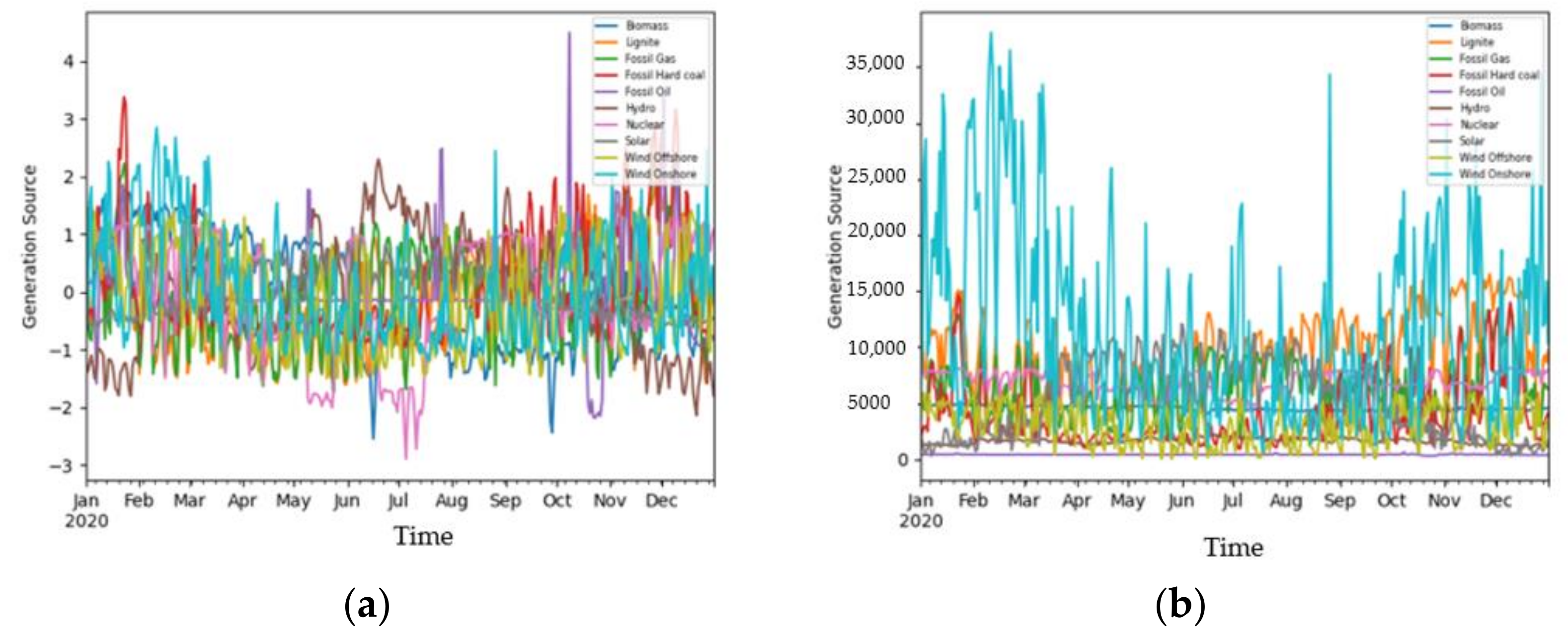
• Compared with France and NO1, Germany has the most diverse energy mix, but is also heavily dependent on the fluctuating energy production from on-shore wind, which accounts for the largest share even before lignite;
• The wide confidence levels could be explained by the strongly fluctuating electricity production via offshore wind;
• Day-ahead and intraday prices diverge sharply in the first half of the year but have converged significantly in the second half of the year;
• The first lockdown shows a fundamentally lower price level than the second. At the same time, the first lockdown is the period with the highest volatility;
• The price level in January 2021 is significantly higher than the price level in January 2020.

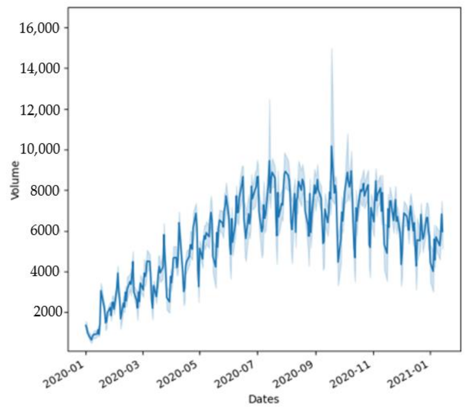
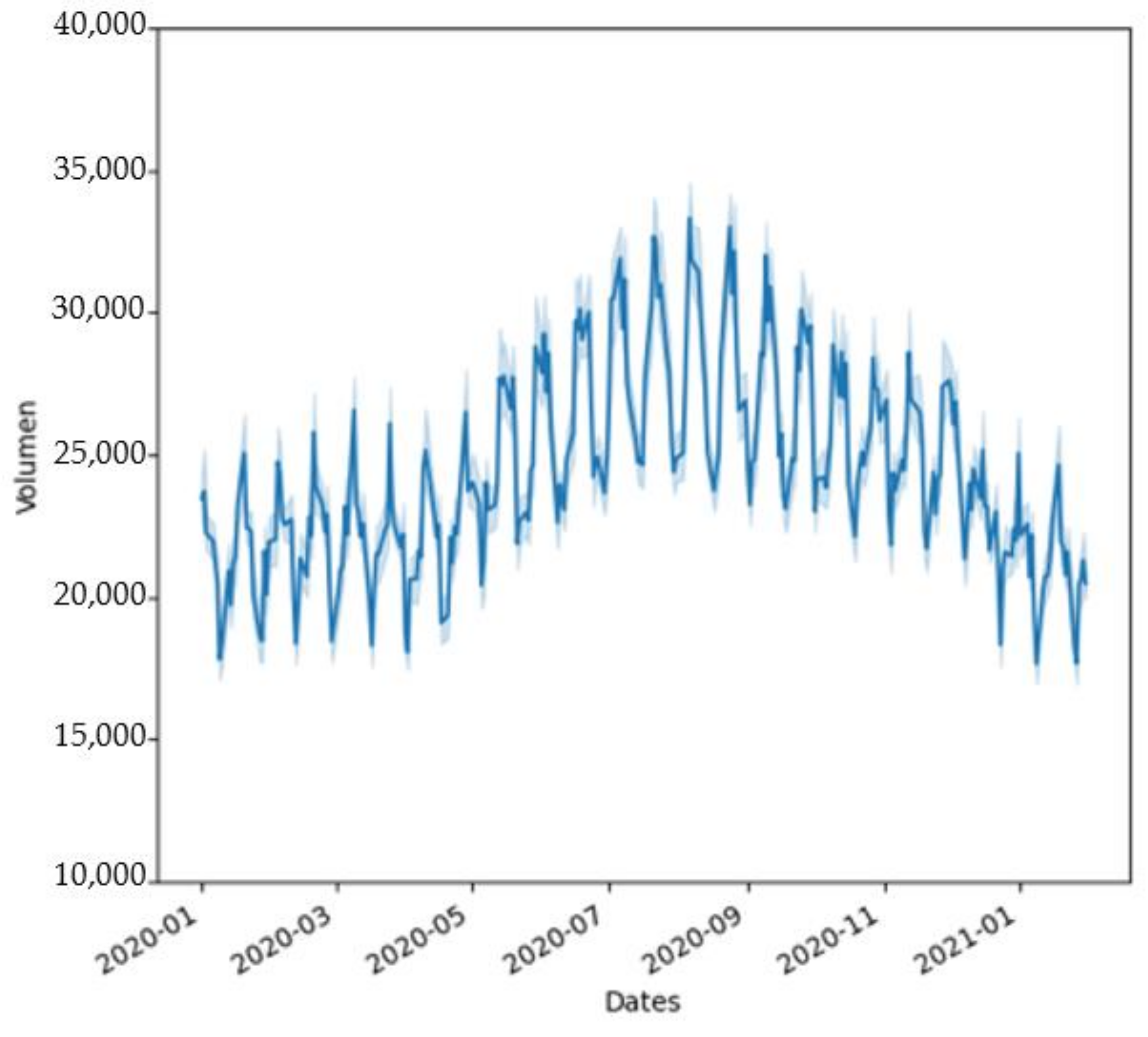
3.2.3. German Traded Volumes

Figure 9 and Figure 10 compare the volumes traded on the German intraday (Figure 9) and day-ahead (Figure 10) markets. When looking at the day-ahead volumes this figure does not indicate any abnormalities during the COVID-19 pandemic crisis. Rather, this figure indicates seasonal fluctuations. In the intraday area, however, the situation is different. The confidence levels show large outliers, especially in the summer months. Higher traded volumes on the intraday market are linked to a higher level of flexibility.

• In January 2020, higher volumes were traded than in January 2021;
• In the first lockdown, the standard deviation in the day-ahead area was higher than in later periods, and more average daily volume was traded in the day-ahead market. It does not decrease again until late summer;
• On the day-ahead market, it is noticeable that the confidence level is always quite constant and that the volumes increase in the summer months;
• In the second lockdown, more was traded in the intraday area/less was traded in the day-ahead area (compared to the first lockdown period).

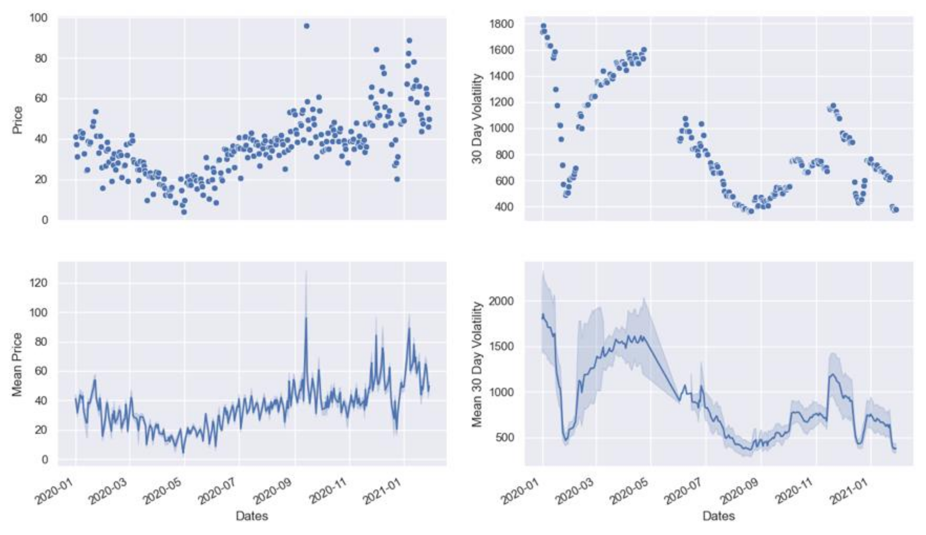
3.3. French Electricity Prices

The graphical analysis follows the same pattern for France. The same parameters are superimposed, and day-ahead and intraday prices are also compared. As each country in Europe has its own lockdown rules, the lockdown periods in France differ from those in Germany. In France, the first lockdown period was from March to June/July. This extends the observation period compared to Germany. The second lockdown began in mid-October and was relaxed again in mid-December. Until the end of our observation period on 1 February, a curfew remained in place from 6 p.m. to 6 a.m. CET [31]. France obtains most of its electricity from nuclear energy sources. The calculations based on the average values showed that almost 70% of the electricity produced over the year came from nuclear sources. Hydropower and onshore wind power take second and third place in France. The mean values of both accounted for less than 10% of the energy mix on an annual average [8].

3.3.1. French Intraday Prices

In direct comparison with the German intraday electricity prices, it is noticeable that the price level of the French intraday prices fluctuates even more (Figure 11). However, the general price level falls between March and May 2020 and rises again in June. Volatility initially fell sharply in February 2020 but jumped again in March, coinciding with the first COVID-19 measures. Volatility in June is lower than in the previous month. The confidence interval of volatility from March to June also indicates a higher dispersion and, thus, greater uncertainty regarding forecasts. As volatility decreases and prices rise in June, the confidence level also decreases. At the time of the announcement of the second national lockdown, prices and volatility rose simultaneously. Also, the confidence level of volatility shows greater excesses. At the end of the second lockdown, there was a clear drop in prices and a jump in volatility. However, the situation recovers quickly thereafter. Compared to prices in January 2020, prices in January 2021 are at a higher level. In contrast, intraday volatility is at a lower level. The highest price in the data set is 328.20 EUR, and the lowest is –25.20 EUR. This indicates outliers, which are also evident in the price range via the confidence level.

3.3.2. French Day-Ahead Prices

The price development in the day-ahead area (Figure 12) hardly differs from the intraday area. Only the confidence intervals are somewhat larger in the intraday area. This becomes visible via the outliers. In the day-ahead area, the lowest price is −8.65 EUR and the highest at 189.25 EUR. Like the intraday area, the prices are lower in summer than winter. A particularly low-price level during the first lockdown should be noted. Compared to the price level in January 2020, the price level in January 2021 is also higher. Differences in intraday prices are visible when it comes to volatility. Volatility is characterized by two peaks during the two lockdowns. First, there was a clear increase in April 2020 and another in June 2020. In the period in between, volatility fell once again. At the same time, the confidence level also decreases during this period. The development of volatility and confidence intervals during the second lockdown shows similarities to the development in the intraday area.

Figure 12. This figure represents the day-ahead price levels for French power including its confidence levels on the left side and the 30-day volatility including its confidence levels on the right side. Figure 7, Figure 8 and Figure 11, Figure 12, Figure 13 and Figure 14 got generated using the same code in Python.

Figure 12. This figure represents the day-ahead price levels for French power including its confidence levels on the left side and the 30-day volatility including its confidence levels on the right side. Figure 7, Figure 8 and Figure 11, Figure 12, Figure 13 and Figure 14 got generated using the same code in Python.

The average price per day was 37.49 EUR; 36.16 EUR and the standard deviation for the entire period was 18.54; 16.97.

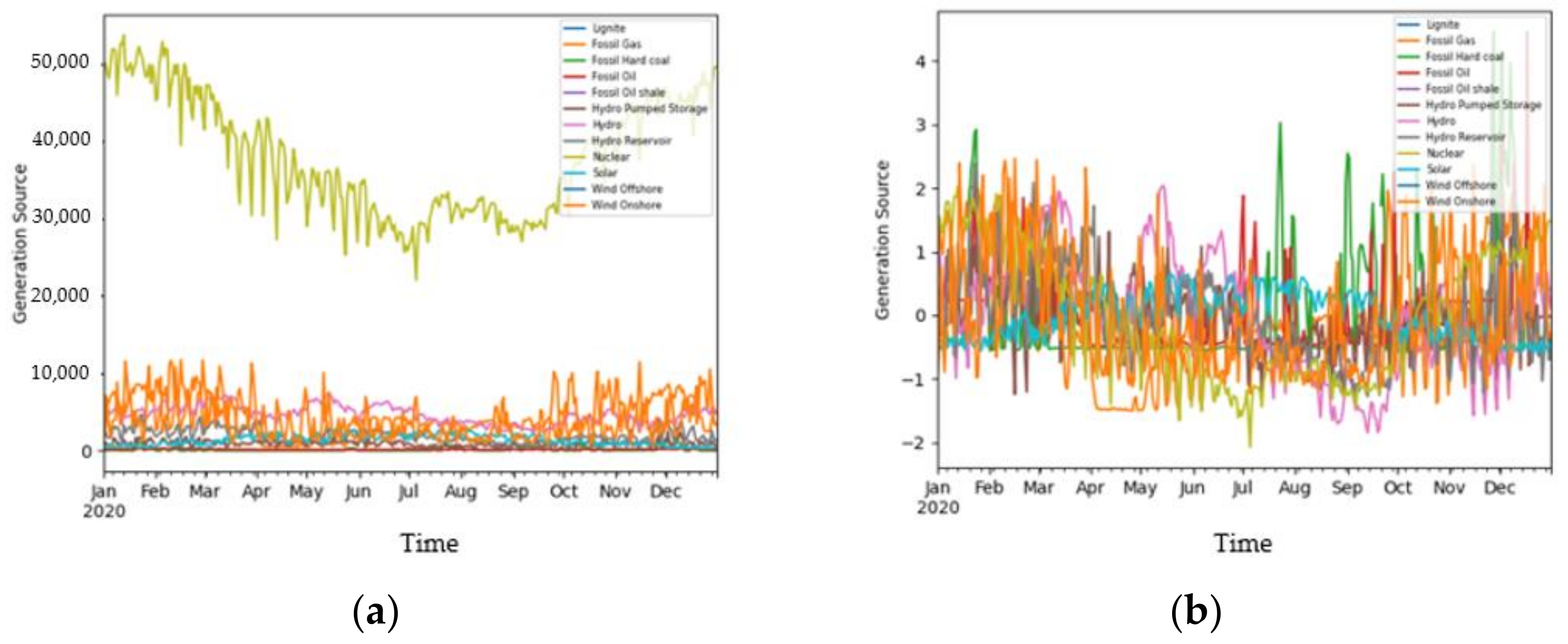
• In France, less nuclear power is produced in the summer months, and a little more use is made of renewable energy sources such as solar. No link between generation and price level is visible;
• Table 5. General Statistics about French Prices and Volatilities in EUR.

  Observation Period	France Intraday (Mean Price; Mean Vola)	France Intraday (Std Price; Std Vola)	France Day-Ahead (Mean Price; Mean Vola)	France Day-Ahead (Std Price; Std Vola)
  January 2020	38.31; 1221.29	12.21; 717.49	37.55; 546.84	10.73; 321.90
  January 2021	62.37; 601.00	18.39; 309.41	61.24; 644.05	17.17; 647.56
  First Lockdown	22.00; 1397.17	9.78; 476.57	21.30; 1161.13	9.32; 795.95
  Second Lockdown	47.09; 843.06	16.76; 405.42	46.26; 824.63	15.41; 651.17
  Summer Months	41.45; 527.49	16.33; 242.01	40.76; 567.71	12.34; 490.50

  shows that there are no major fluctuations between day-ahead and intraday. Thus, it can be said for the forecast accuracy that it is higher in France;
• In the first lockdown, prices fell sharply and showed a high volatility. In the second lockdown, prices rose sharply, and volatility was low;
• Day-ahead and intraday prices were always close to each other in the mean and median. However, they also show strong outliers.

3.3.3. French Traded Volumes

The following is a brief supporting analysis of the volumes for French electricity prices.

Table 6. General Statistics about French Volumes in MWh.

Observation Period	France Intraday (Mean)	France Intraday (Std)	France Day-Ahead (Mean)	France Day-Ahead (Std)
January 2020	178.21	292.91	14,724.14	2855.71
January 2021	178.99	257.54	16,449.86	2642.51
First Lockdown	132.13	244.21	14,088.72	2381.12
Second Lockdown	195.73	309.71	14,373.57	2600.35
Summer Months	180.25	288.66	12,450.08	2650.61

represents the general statistics regarding the traded volumes. Thereby, the analysis was conducted on the mean and standard deviation for intraday and day-ahead prices. The average volume traded per day was 169.43 MWh; 14,082.17 MWh and the standard deviation for the entire period was 288.43; 2814.81.

• During the first lockdown, less than normal trading took place on the intraday market;
• During the second lockdown, the most trading took place on the intraday market. The standard deviation was also above average;
• During the summer months, less than average was traded via the day-ahead market;
• In January 2021, more than the average was traded on the day-ahead market and more compared to the previous year;
• The standard deviation of the day-ahead volumes is quite constant.

3.4. Norwegian Electricity Prices

The graphical analysis follows the same pattern for Norway. It only considers the Oslo region (NO1). The Norwegian government declared a national lockdown in mid-March 2020. At the end of April, the first relaxations were decided, and relaxations were introduced until mid-June [32]. Norway introduced new national restrictions by the end of October 2020. These restrictions were still in place once the observation period ended [33]. In terms of energy production, Norway produces electricity mainly from hydropower. This energy source is divided into the hydro water reservoir and hydro run-of-river and poundage. Together, these two energy sources account for almost 100% on an annual average. Wind onshore or fossil gas accounts for less than 5% of Norway’s energy production [8].

3.4.1. NO1 Intraday Prices

The price development in the intraday area (Figure 13) shows a bearish trend, including several outliers until April. At the beginning of June, the price level was relatively stable at EUR 9.00. During the second lockdown period, the prices show volatile movements. The trend is a rising price. Compared to the price level in January 2020, the price level in January 2021 was higher. However, the curve shows a high price level in winter and a low price level in summer. The confidence level of the prices does not show any conspicuous features and is evenly distributed over the year. The lowest price in the data set here is −1.73 EUR, and the highest price is 205.68 EUR. The 30-day volatility also increased during the first lockdown period. Thus, it started being around 350 in the first lockdown and ended up at a level of 770 during the second lockdown. The confidence level of the 30-day volatility increased between March and July and decreased again in September. The second lockdown also shows a widened confidence level.

Figure 13. This figure represents the intraday price levels for NO1 power including its confidence levels on the left side and the 30-day volatility including its confidence levels on the right side. Figure 7, Figure 8 and Figure 11, Figure 12, Figure 13 and Figure 14 got generated using the same code in Python.

Figure 13. This figure represents the intraday price levels for NO1 power including its confidence levels on the left side and the 30-day volatility including its confidence levels on the right side. Figure 7, Figure 8 and Figure 11, Figure 12, Figure 13 and Figure 14 got generated using the same code in Python.

3.4.2. NO1 Day-Ahead Prices

The price development in the day-ahead area (Figure 14) also shows a bearish trend until April. Like in the intraday area, the prices reached their lowest point in June. From June, the day remained at nearly the same level. During the summer months, the price level remained low and showed some peaks in September and November. In December, the price level increased again. Compared to January 2020, the price level was higher in January 2021 (

Table 7. General Statistics about NO1 Prices and Volatilities in EUR.

Observation Period	NO1 Intraday (Mean Price; Mean Vola)	NO1 Intraday (Std Price; Std Vola)	NO1 Day-Ahead (Mean Price; Mean Vola)	NO1 Day-Ahead (Std Price; Std Vola)
January 2020	25.34; 160.33	4.19; 100.58	23.68; 97.94	4.06; 29.08
January 2021	59.16; 575.52	28.79; 124.94	52.41; 539.61	19.25; 162.48
First Lockdown	8.96; 354.71	4.86; 178.76	7.79; 193.10	2.05; 76.19
Second Lockdown	28.86; 773.76	28.10; 332.86	26.10; 688.65	22.98; 365.61
Summer Months	5.47; 620.98	5.20; 299.48	4.71; 419.00	4.65; 272.55

). Regarding the confidence level of the prices, there are no conspicuous features in the day-ahead area. This indicates that the uncertainty regarding prices is less great. In the day-ahead area, the curve also shows a low price level in summer and a high price level in winter. In terms of this shape, there is a similarity to the intraday prices. The lowest price in the data set is 0.02 EUR, and the highest price is 152.25 EUR. At the end of March, volatility started increasing and reached the first peak in the mid of April where it remained relatively stable. The volatility shows more peaks between May and October. In November, it started to rise and ended up at a higher level compared to January 2020. Between November and March, the confidence level widened until it narrowed again in January.

Figure 14. This figure represents the day-ahead price levels for NO1 power including its confidence levels on the left side and the 30-day volatility including its confidence levels on the right side. Figure 7, Figure 8 and Figure 11, Figure 12, Figure 13 and Figure 14 got generated using the same code in Python.

Figure 14. This figure represents the day-ahead price levels for NO1 power including its confidence levels on the left side and the 30-day volatility including its confidence levels on the right side. Figure 7, Figure 8 and Figure 11, Figure 12, Figure 13 and Figure 14 got generated using the same code in Python.

The average price of the daily traded volume was 14.17 EUR for intraday and 12.72 EUR for day-ahead prices. The standard deviation was 17.65 for intraday and 14.82 for day-ahead.

• During the first lockdown, the price in the day-ahead and intraday area fell sharply. This trend was reinforced in the summer months. In the summer months, less electricity was produced by waste and wind power;
• In the second lockdown, the price level and the level of volatility increased. At the beginning of the second lockdown, the production of hydropower by water reservoirs collapsed;
• The price level in January 2021 is significantly higher than the price level in January 2020. The same applies to volatility;
• Intraday and day-ahead prices both have low confidence level shears and have a similar shape (low prices in summer and high prices in winter);
• There are no strong outliers, as is the case with German and French prices. Intraday prices show more outliers than Day-Ahead prices;
• Hydropower as the largest generation source can be stored and is more independent of the weather;
• Both curves show very similar price and volatility developments.

The results confirm the statement that the 2nd lockdown had a stronger impact on the energy markets in the NO1 region.

4. Discussion

4.1. Critical Appraisal

The following section discusses elements of the paper based on the current state of research. Since a further step in analyzing the data would be prediction methods, we will now briefly discuss back testing, which is commonly used in practice. We can refer to the study by L. Han et al. (2020). They pointed out that spot electricity prices are among the financial products with the highest price deviations and the greatest volatility. They attribute this to the non-storable nature of electricity [13]. Due to the many uncertainties caused by the high volatilities and the price outliers, increasingly complex technologies are being used in the energy markets to predict prices [13,34]. This is necessary because errors arise, for example, through back testing. This is the case because back testing cannot detect so-called black swans [35,36]. An example of a so-called black swan event was the negative oil prices in April 2020 [5,36]. Machine learning (ML) can get around this problem. For example, multivariate analyses using ML can be used to find important indicators that point to a crisis [35]. Different energy markets would support the research here. Therefore, we recommend ML techniques for further analysis of the data.

Another challenge regarding the forecasting accuracy of German electricity is the rapidly changing energy mix. The higher volatilities caused by this also require further complex models and automated trading techniques. In addition, there is a growing need for more comprehensive analyses of alternative data types, such as weather [4,6,37]. This alternative data type is an additional element of the analysis compared to the financial markets. O. B. Adekoya and J.A. Oliyide (2021) and A. Elsayed et al. (2020) have highlighted the links between financial markets and other commodities during the COVD-19 crisis. This comparison is not made in this paper, as the focus is on pure price and volatility movements, supported in some cases by volume data [10,12]. J. Ali, W. Kahn (2020) analyzed the markets according to the lockdown periods [9]. The same procedure was used in this paper. However, weaknesses of the method have become apparent since, in a comprehensive comparison of countries, the lockdown periods differ due to national regulations [25,29,31,33]. This leads to more difficult comparability of the data. However, we have deliberately decided to extend the analysis to include different countries and, in contrast to S. Halbrügge et al. (2021) and C. Fezzi and V. Fanghella (2020), to carry out a country comparison [4,14]. Furthermore, this analysis should draw attention to the growing importance of the intraday electricity markets during the expansion of renewable energies [19,38]. In this way, links to the energy mixes of the countries and the response to COVID-19 can be established.

N. Löhndorf and D. Wozabal have shown in the course of their research why the intraday and day-ahead markets are interdependent and why trading only on one of the markets would not make sense. For example, it would not be optimal to fully utilize the capacity of the day-ahead market without leaving capacity for the intraday markets. They point out that the attractiveness of the intraday markets lies in their volatility and information content. They assume that the attractiveness of the day-ahead markets lies in the market department. According to their research, forecast errors in the day-ahead market can be caused by e.g., wrong weather forecasts. These forecast errors then trigger, among other things, price changes in the intraday markets [28,39].

4.2. Research Limitations

This paper refers to forecasting accuracy when the price difference between the intraday and the day-ahead electricity markets are described. However, the prevailing research contradicts the term forecast accuracy is a precise term to describe the price differences between day-ahead and intraday markets. As some bidders perform price arbitrage between day-ahead and intraday markets to maximize profits, the day-ahead price is not often a forecast of the intraday price [40,41]. In order to obtain even more valid results, factors such as weather, seasonal fluctuations and correlations with other commodities, and, if applicable, public holidays would also have to be considered. Furthermore, the data quality of the Norwegian data is limited as there is no volume data available on Bloomberg. For further analyses, it would therefore be helpful to draw on other Nordic markets and more regions in Norway with a high share of renewable energies as well. Sweden or Denmark, for example, could be considered [22]. This paper does not consider different price systems. For instance, in Europe and Australia, a zonal price system is common, whereas the U.S. uses a nodal price system. In the case of a wider selection of countries, these differences need to be considered [42]. In addition to it, we only considered the market closing prices of each day under consideration. In order to draw a conclusion on intraday volatility, hourly price data should be included as it might have had a positive impact on the data quality. We did include weather forecasts in our analysis as done by Kuppelwieser and Wozabal (2021) [7]. An additional factor that could be considered is the COVID-19 case numbers or, in the meantime, the vaccination rate for the countries studied.

5. Conclusions and Outlook

This paper finds that COVID-19 had an impact on the energy markets in Germany, France, and Norway (NO1). The German electricity market is facing changes. Due to the increase in energy production from renewable energies, more and more energy is being traded on the intraday market [39]. This trend is confirmed by our analysis of the volume. Our overall objective was to determine whether (iii) forecasting methods in intraday electricity markets in Germany have improved. To find out, we compared day-ahead prices and intraday prices. We did this because the day-ahead price is the market-clearing price [38,42,43]. In the comparison, we found that prices in France and Norway were consistently close. (ii) The power generation in France, which consists mainly of nuclear electricity, gives a hint here. We conclude that France shows close intraday and day-ahead prices. This may be due to the constant use of nuclear power. We had expected that (ii, iii) Norway would also be highly efficient. Based on our analysis, we can conclude that the intraday and day-ahead prices are close together. Norway seems to be an exception here. Based on our data NO1 data, we can conclude they have low prices and hardly any outliers, which is particularly evident in the first lockdown period when compared to the developments of the German and France day-ahead and intraday markets. Regarding the day-ahead data, the 30-day volatilities were consistently lower than in Germany and France. These findings provide an indication of the link to the increased use of hydropower and hydro reservoirs in Norway (NO1) [8]. In Germany, prices were initially far apart during the first lockdown period. During the second lockdown period, there was a convergence of prices in the mean and median. This convergence is (i) an indication, but not proof, that the use of the out-of-sample data of the first lockdown may have improved the forecast accuracy. In addition, (iii) the constantly changing energy mix in Germany may have played a role. The results for the German market could be used as pioneering data for other countries that want to undertake such an energy transition [39]. Other results are as follows:

• All products considered show a higher price in January 2021 compared to the previous year;
• In the case of German electricity, however, a lower daily average volume was traded in January 2021 compared to the previous year. The volume in France remains constant in the intraday area and is increased in the day-ahead area;
• All prices considered fell in the first lockdown, whereas volatilities rose sharply in some cases;
• In contrast to France and Germany, the electricity prices for NO1 show fewer outliers, which could be explained by the generation from water reservoirs and hydropower;
• All prices increased in the second lockdown. Unlike the other products, the volatility of NO1 increased particularly strongly in the second lockdown. This suggests that NO1 was hit harder by the second lockdown than by the first.

In the general price and volatility analysis, it was determined that the weather factor was omitted in the case of nuclear electricity and electricity from hydropower, which could lead to higher forecast accuracy and to greater crisis security. Higher forecast accuracy is becoming more important because of extreme electricity prices that have occurred with larger magnitude and higher frequency in recent years [44]. In addition, new market regulations and cross-country interconnections need to be considered to understand electricity prices [45]. Macroeconomic events can lead to an increased level of uncertainty in the natural gas and electricity market [46,47]. Furthermore, the aim of our research is to provide statistical evidence for the relationship between energy production and price and volatility movements. We want to do this because this paper only makes assumptions based on the results of the graphical analysis.

To produce more valid results, we plan to expand the dataset and consider further crisis periods. Thus, potential future research would include generalizable indicators from the prevailing time series that could be employed to filter out or predict future crisis situations. Reference data for validation could be price data during the Russian aggression against Ukraine or the subprime crisis. Such a model should be possible even though there are different energy mixes and or other special features regarding the data structure, e.g., different lockdown periods. The overall research goal is to develop methods that can predict the crisis or key indicators such as volatility.

References

1. Marshman, D.; Brear, M.; Jeppesen, M.; Ring, B. Performance of wholesale electricity markets with high wind penetration. Energy Econ. 2020, 89, 104803. [Google Scholar] [CrossRef]
2. Detemple, J.; Kitapbayev, Y. The value of green energy under regulation uncertainty. Energy Econ. 2020, 89, 104807. [Google Scholar] [CrossRef]
3. Härtel, P.; Korpås, M. Demystifying market clearing and price setting effects in low-carbon energy systems. Energy Econ. 2020, 93, 105051. [Google Scholar] [CrossRef]
4. Halbrügge, S.; Schott, P.; Weibelzahl, M.; Buhl, H.U.; Fridgen, G.; Schöpf, M. How did the German and other European electricity systems react to the COVID-19 pandemic? Appl. Energy 2021, 285, 116370. [Google Scholar] [CrossRef]
5. Ghiani, E.; Galici, M.; Mureddu, M.; Pilo, F. Impact on Electricity Consumption and Market Pricing of Energy and Ancillary Services during Pandemic of COVID-19 in Italy. Energies 2020, 13, 3357. [Google Scholar] [CrossRef]
6. Duso, T.; Szücs, F.; Böckers, V. Abuse of dominance and antitrust enforcement in the German electricity market. Energy Econ. 2020, 92, 104936. [Google Scholar] [CrossRef]
7. Kuppelwieser, T.; Wozabal, D. Intraday Power Trading: Towards an Arms Race in Weather Forecasting? Eur. J. Oper. Res. 2021, in press. [Google Scholar]
8. ENTSO-E. Actual Generation per Production Type. Available online: https://transparency.entsoe.eu/generation/r2/actualGenerationPerProductionType/show (accessed on 5 June 2021).
9. Ali, J.; Khan, W. Impact of COVID-19 pandemic on agricultural wholesale prices in India: A comparative analysis across the phases of the lockdown. Public Aff. 2020, 20, e2402. [Google Scholar] [CrossRef]
10. Elsayed, A.H.; Nasreen, S.; Tiwari, A.K. Time-varying co-movements between energy market and global financial markets: Implication for portfolio diversification and hedging strategies. Energy Econ. 2020, 90, 104847. [Google Scholar] [CrossRef]
11. Bompard, E.; Mosca, C.; Colella, P.; Antonopoulos, G.; Fulli, G.; Masera, M.; Poncela-Blanco, M.; Vitiello, S. The Immediate Impacts of COVID-19 on European Electricity Systems: A First Assessment and Lessons Learned. Energies 2020, 14, 96. [Google Scholar] [CrossRef]
12. Adekoya, O.B.; Oliyide, J.A. How COVID-19 drives connectedness among commodity and financial markets: Evidence from TVP-VAR and causality-in-quantiles techniques. Resour. Policy 2020, 70, 101898. [Google Scholar] [CrossRef] [PubMed]
13. Han, L.; Kordzakhia, N.; Trück, S. Volatility spillovers in Australian electricity markets. Energy Econ. 2020, 90, 104782. [Google Scholar] [CrossRef]
14. Fezzi, C.; Fanghella, V. Real-Time Estimation of the Short-Run Impact of COVID-19 on Economic Activity Using Electricity Market Data. Environ. Resour. Econ. 2020, 76, 885–900. [Google Scholar] [CrossRef] [PubMed]
15. Kath, C.; Ziel, F. The value of forecasts: Quantifying the economic gains of accurate quarter-hourly electricity price forecasts. Energy Econ. 2018, 76, 411–423. [Google Scholar] [CrossRef] [Green Version]
16. Kath, C.; Ziel, F. Conformal prediction interval estimation and applications to day-ahead and intraday power markets. Int. J. Forecast. 2021, 37, 777–799. [Google Scholar] [CrossRef]
17. Finnah, B.; Gönsch, J.; Ziel, F. Integrated day-ahead and intraday self-schedule bidding for energy storage systems using approximate dynamic programming. Eur. J. Oper. Res. 2021, 301, 726–746. [Google Scholar] [CrossRef]
18. Maciejowska, K.; Nitka, W.; Weron, T. Day-Ahead vs. Intraday—Forecasting the Price Spread to Maximize Economic Benefits. Energies 2019, 12, 631. [Google Scholar] [CrossRef] [Green Version]
19. Kramer, A.; Kiesel, R. Exogenous factors for order arrivals on the intraday electricity market. Energy Econ. 2021, 97, 105186. [Google Scholar] [CrossRef]
20. Ghosh, S.; Bohra, A.; Dutta, S. The Texas Freeze of February 2021: Event and Winterization Analysis Using Cost and Pricing Data. In Proceedings of the IEEE Electrical Power and Energy Conference (EPEC), Toronto, ON, Canada, 22–31 October 2021; IEEE: Piscataway, NJ, USA; pp. 7–13. [Google Scholar] [CrossRef]
21. Xiao, D.; AlAshery, M.K.; Qiao, W. Optimal price-maker trading strategy of wind power producer using virtual bidding. J. Mod. Power Syst. Clean Energy 2021, 1–13. [Google Scholar] [CrossRef]
22. Snow, D. Machine Learning in Asset Management. SSRN Electron. J. 2019. [Google Scholar] [CrossRef]
23. Rintamäki, T.; Siddiqui, A.S.; Salo, A. Does renewable energy generation decrease the volatility of electricity prices? An analysis of Denmark and Germany. Energy Econ. 2017, 62, 270–282. [Google Scholar] [CrossRef] [Green Version]
24. Cramton, P. Electricity market design. Oxf. Rev. Econ. Policy 2017, 33, 589–612. [Google Scholar] [CrossRef] [Green Version]
25. Malec, M.; Kinelski, G.; Czarnecka, M. The Impact of COVID-19 on Electricity Demand Profiles: A Case Study of Selected Business Clients in Poland. Energies 2021, 14, 5332. [Google Scholar] [CrossRef]
26. Pilipović, D. Energy Risk; McGraw-Hill: New York, NY, USA, 1998; pp. 100–101. [Google Scholar]
27. Verbeek, M. Modern Econometrics, 5th ed.; Wiley Custom: Croydon, UK, 2017; pp. 167–173. [Google Scholar]
28. Löhndorf, N.; Wozabal, D. The Value of Coordination in Multimarket Bidding of Grid Energy Storage. Work. Pap. 2021. [Google Scholar] [CrossRef]
29. Robert Koch Institut. Available online: https://www.rki.de/DE/Content/InfAZ/N/Neuartiges_Corona-virus/nCoV_node.html (accessed on 5 June 2021).
30. Valitov, N.; Maier, A. Asymmetric information in the German intraday electricity market. Energy Econ. 2020, 89, 104785. [Google Scholar] [CrossRef]
31. Governement. Available online: https://www.gouvernement.fr/en/coronavirus-covid-19 (accessed on 5 June 2021).
32. Ursin, G.; Skjesol, I.; Tritter, J. The COVID-19 pandemic in Norway: The dominance of social implications in framing the policy response. Health Policy Technol. 2020, 9, 663–672. [Google Scholar] [CrossRef]
33. Government.no. URL. Available online: https://www.regjeringen.no/en/topics/koronavirus-covid-19/id2692388/ (accessed on 5 June 2021).
34. Wang, B.; Wang, J. Energy futures and spots prices forecasting by hybrid SW-GRU with EMD and error evaluation. Energy Econ. 2020, 90, 104827. [Google Scholar] [CrossRef]
35. Se Prado, M.M.L. Machine Learning for Asset Managers; Cambridge University Press: Cambridge, UK, 2020; pp. 19–20. [Google Scholar]
36. Selmi, R.; Bouoiyour, J.; Hammoudeh, S. Negative Oil: Coronavirus, a “Black Swan” Event for the Industry? 2020. Available online: https://hal.archives-ouvertes.fr/hal-02570614/document (accessed on 5 June 2021).
37. Agnello, L.; Castro, V.; Hammoudeh, S.; Sousa, R.M. Global factors, uncertainty, weather conditions and energy prices: On the drivers of the duration of commodity price cycle phases. Energy Econ. 2020, 90, 104862. [Google Scholar] [CrossRef]
38. Glas, S.; Kiesel, R.; Kolkmann, S.; Kremer, M.; Von Luckner, N.G.; Ostmeier, L.; Urban, K.; Weber, C. Intraday renewable electricity trading: Advanced modeling and numerical optimal control. J. Math. Ind. 2020, 10, 3. [Google Scholar] [CrossRef]
39. Kiesel, R.; Paraschiv, F. Econometric analysis of 15-minute intraday electricity prices. Energy Econ. 2017, 64, 77–90. [Google Scholar] [CrossRef] [Green Version]
40. Hadsell, L. The impact of virtual bidding on price volatility in New York’s wholesale electricity market. Econ. Lett. 2007, 95, 66–72. [Google Scholar] [CrossRef]
41. Iria, J.; Soares, F.; Matos, M. Optimal supply and demand bidding strategy for an aggregator of small prosumers. Appl. Energy 2018, 213, 658–669. [Google Scholar] [CrossRef]
42. Grimm, V.; Rückel, B.; Sölch, C.; Zöttl, G. The impact of market design on transmission and generation investment in electricity markets. Energy Econ. 2020, 93, 104934. [Google Scholar] [CrossRef]
43. De Lagarde, C.M.; Lantz, F. How renewable production depresses electricity prices: Evidence from the German market. Energy Policy 2018, 117, 263–277. [Google Scholar] [CrossRef]
44. Liu, L.; Bai, F.; Su, C.; Ma, C.; Yan, R.; Li, H.; Sun, Q.; Wennersten, R. Forecasting the occurrence of extreme electricity prices using a multivariate logistic regression model. Energy 2022, 247, 123417. [Google Scholar] [CrossRef]
45. Tschora, L.; Pierre, E.; Plantevit, M.; Robardet, C. Electricity price forecasting on the day-ahead market using machine learning. Appl. Energy 2022, 313, 118752. [Google Scholar] [CrossRef]
46. Shi, X.; Shen, Y. Macroeconomic uncertainty and natural gas prices: Revisiting the Asian Premium. Energy Econ. 2020, 94, 105081. [Google Scholar] [CrossRef]
47. Moutinho, V.; Oliveira, H.; Mota, J. Examining the long term relationships between energy commodities prices and carbon prices on electricity prices using Markov Switching Regression. Energy Rep. 2022, 8, 589–594. [Google Scholar] [CrossRef]
Figure 1. This figure represents the German electricity spot market. This figure functions to improve understanding on the market design. This figure has been presented according to Kramer and Kiesel (2021) [19].
Energies 15 03494 g001
Figure 2. This figure represents the research design including the different stages of research the data went through in the course of the analysis. The extent at which each kind of data got analyzed has been linked to the data availability in Bloomberg. DA = day-ahead, I = intraday, p = Price, v = volume.
Energies 15 03494 g002
Figure 3. This figure represents the German electricity generation. (a) Shows an approach using data standardization which has been defined in Formula (3); (b) Shows the electricity generation sources in MWh. Figure 3, Figure 4 and Figure 5 got generated using the same code in Python.
Energies 15 03494 g003
Figure 4. This figure represents the French electricity generation. (a) Shows an approach using data standardization which has been defined in Formula (3); (b) Shows the electricity generation sources in MWh. Figure 3, Figure 4 and Figure 5 got generated using the same code in Python.
Energies 15 03494 g004
Figure 5. This figure represents the Norway (NO1) electricity generation. (a) Shows an approach using data standardization which has been defined in Formula (3); (b) Shows the electricity generation sources in MWh. Figure 3, Figure 4 and Figure 5 got generated using the same code in Python.
Energies 15 03494 g005
Figure 6. These figures show an example of the German day-ahead prices (a) and intraday prices (b). The visualization applies standardized data (see Formula (3)). Figure 6 got generated using the same code in Python.
Energies 15 03494 g006
Figure 7. This figure represents the intraday price levels for German power including its’ confidence levels on the left side and the 30 day volatility including its’ confidence levels on the right side. Figure 7 and Figure 8 got generated using the same code in Python.
Energies 15 03494 g007
Figure 8. This figure represents the day-ahead price levels for German power including its’ confidence levels on the left side and the 30-day volatility including its confidence levels on the right side. Figure 7 and Figure 8 were generated using the same code in Python.
Energies 15 03494 g008
Figure 9. Shows German average traded volumes per day in Intraday markets. The light blue shadow represents the 95% confidence level. Figure 9 and Figure 10 got generated using the same code in Python.
Energies 15 03494 g009
Figure 10. Shows German average traded volumes per day in Day-Ahead markets. The light blue shadow represents the 95% confidence level. Figure 9 and Figure 10 got generated using the same code in Python.
Energies 15 03494 g010
Figure 11. This figure represents the intraday price levels for French power including its confidence levels on the left side and the 30-day volatility including its confidence levels on the right side. Figure 7, Figure 8 and Figure 11, Figure 12, Figure 13 and Figure 14 got generated using the same code in Python.
Energies 15 03494 g011