Development of a Permeability Formula for Tight and Shale Gas Reservoirs Based on Advanced High-Precision Lab Measurement Techniques
Abstract
1. Introduction
2. Materials and Methods
2.1. Material Description
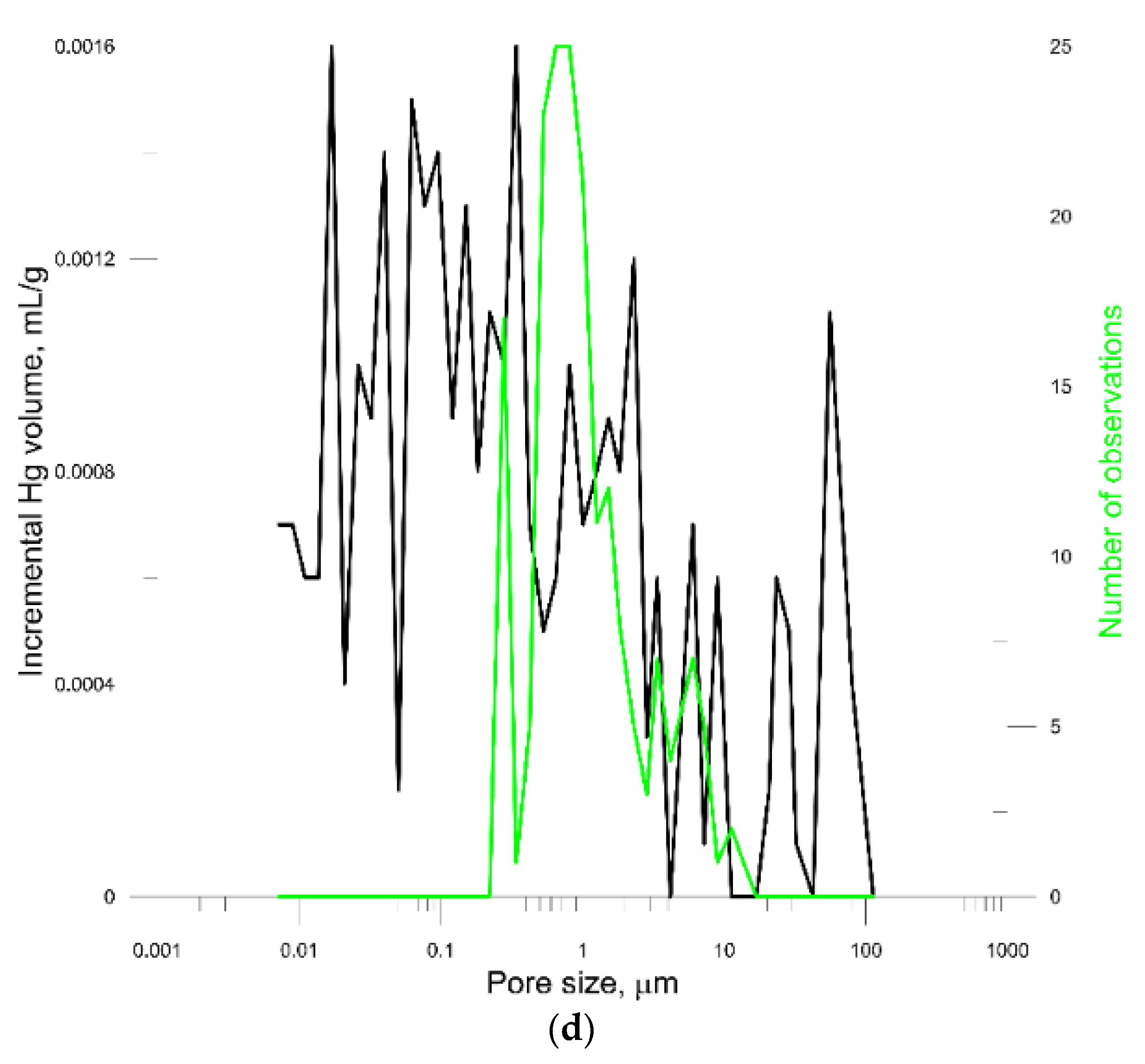
2.2. Mercury Injection Capillary Pressure Method
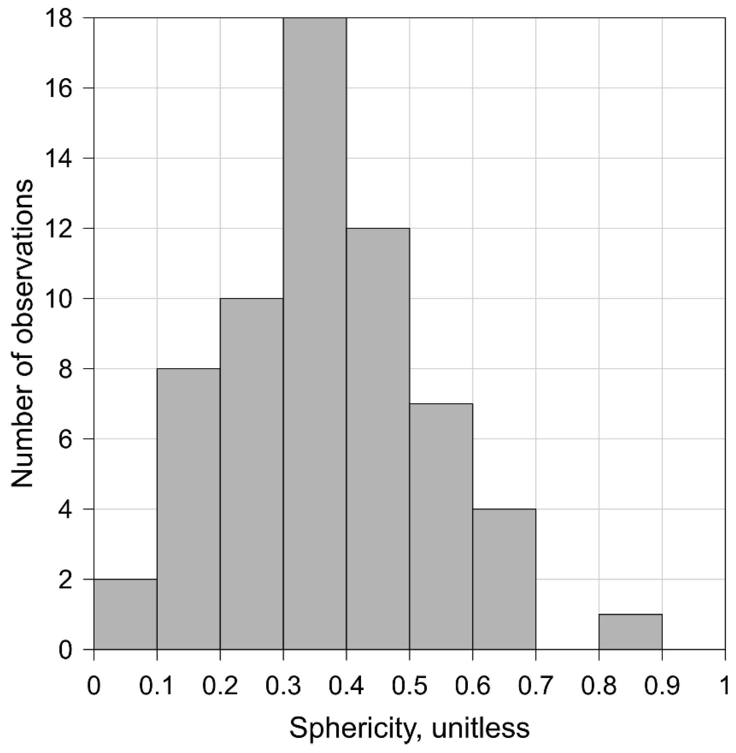
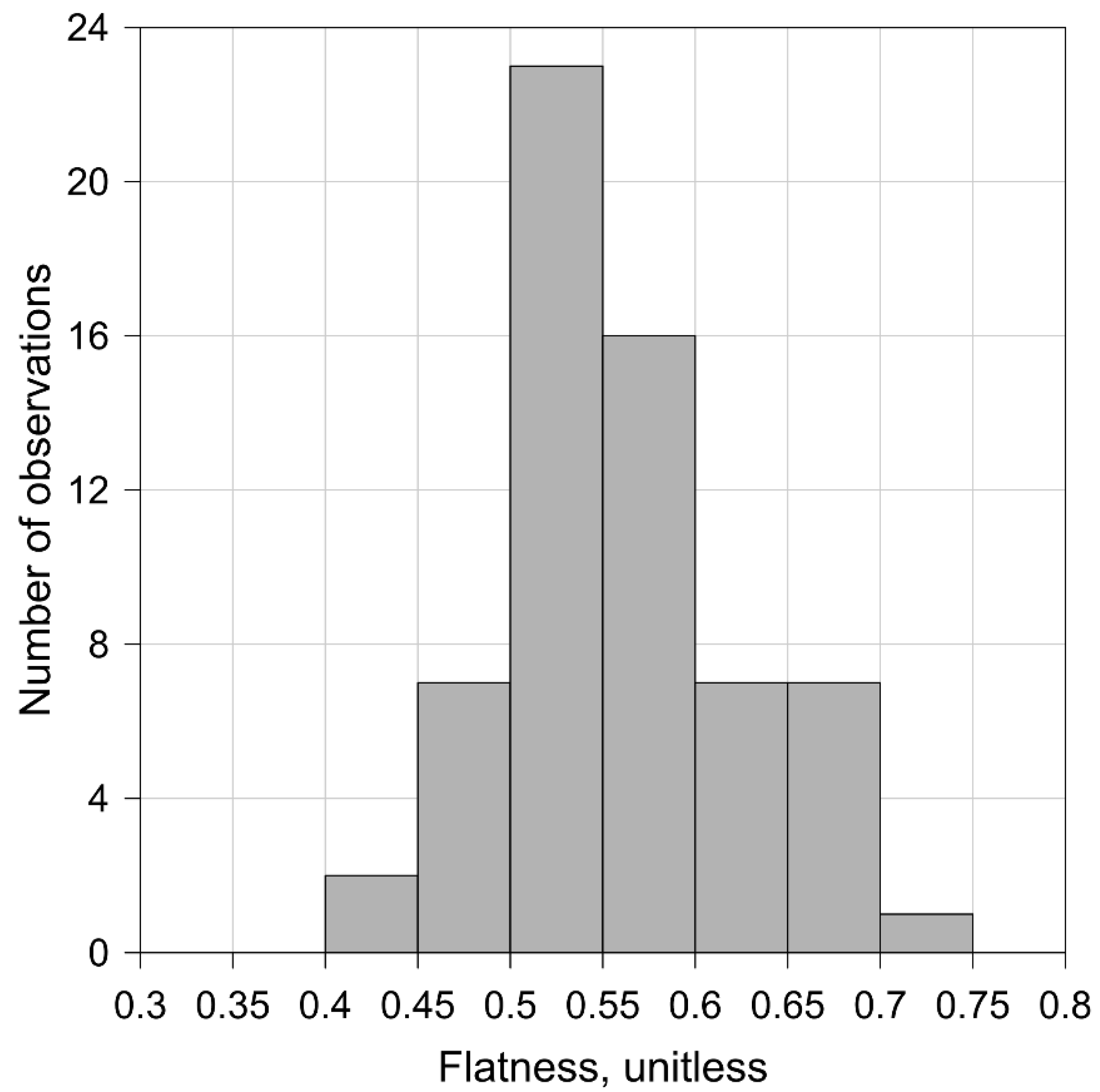
2.3. Computed X-ray Tomography Method
2.4. Pulse and Pressure Decay Permeability Method
2.5. Multiple Linear Regression Analysis
2.6. Stages of the Analysis
- (1)
- calculate the geometrical parameters for each object (pore, microfracture) in each sample (parameters in Table 2 and their quotients) and the porosity;
- (2)
- quality check (check the value correctness in the range, e.g., 0–1, and interpretable values, i.e., whether the value has a physical meaning) the parameters for each of the 62 samples;
- (3)
- calculate the statistics: maximum, minimum, average, standard deviation, median, 10th percentile, 90th percentile, lower quartile, and upper quartile based on the parameters from all the objects (pores, microfractures) in each sample, e.g., calculate the average thickness (parameter) of all the objects in each sample (finally, 1 sample corresponds to 1 value of a parameter);
- (4)
- extract the parameters for the largest object in each of the 62 samples;
- (5)
- construct the data set: one data set consists of a particular statistical parameter, which is calculated for each sample and all the available parameters from CT, e.g., the data set of the average values of each sample and all the parameters calculated from CT;
- (6)
- analyze the relationships between the absolute permeability from laboratory measurements and the 291 parameters from the CT images (based on their correlation coefficients); only the parameter that correlates with the logarithm of absolute permeability with a correlation coefficient above ±0.5 is considered;
- (7)
- construct a data set from the parameters that showed a linear relationship (correlate) with the logarithm of permeability (reject insignificant parameters);
- (8)
- perform multiple linear regression analysis on the data set from item 7 (parameters that correlate with the logarithm of absolute permeability).
3. Results and Discussion
3.1. Basic Analysis
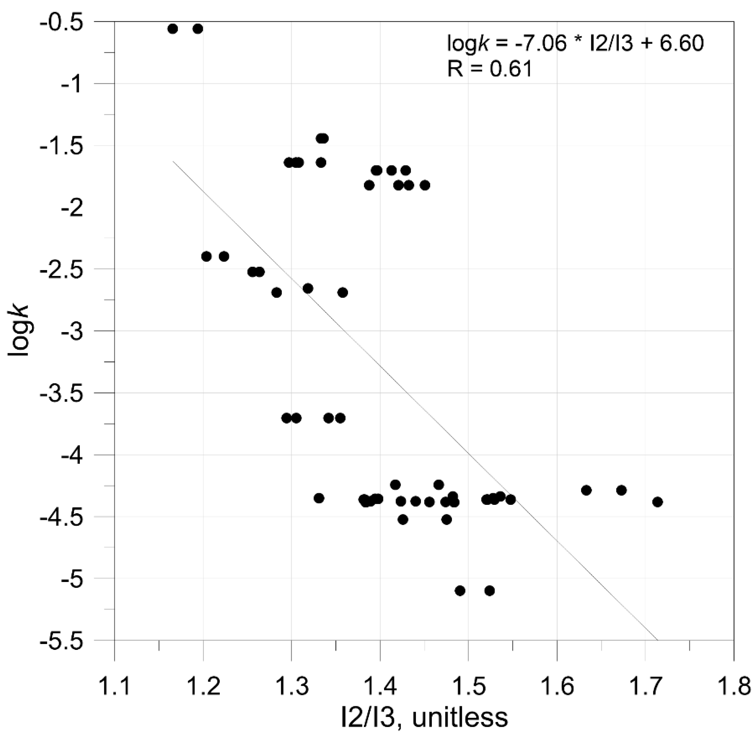
3.2. Linear Relationships between the Logarithm of Absolute Permeability and CT Parameters
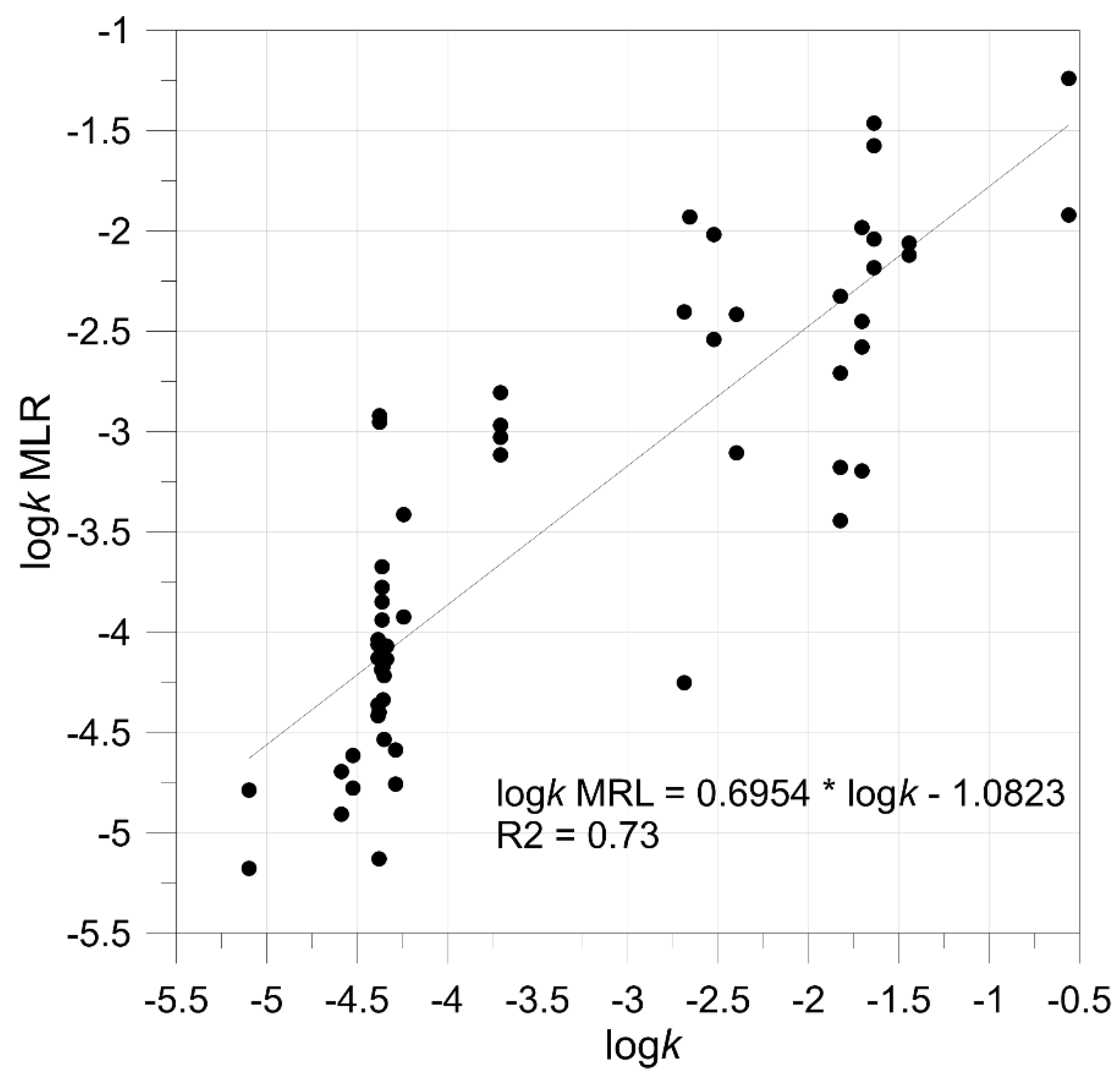
3.3. Multiple Linear Regression Analysis
4. Conclusions
Author Contributions
Funding
Institutional Review Board Statement
Informed Consent Statement
Data Availability Statement
Acknowledgments
Conflicts of Interest
Appendix A
| Sample | CT Porosity for Sample | Volume | Surface Area | Equivalent Diameter | Thickness Max | Thickness Mean | Thickness StD | Anisotropy | Elongation | Flatness | Shericity | Euler Sum | Feret Min | Feret Max | Feret Breadth | Feret Shape | Shape Va3D | I1 | I2 | I3 | GU, Age, Lithology |
|---|---|---|---|---|---|---|---|---|---|---|---|---|---|---|---|---|---|---|---|---|---|
| % | voxels | px2 | px | px | px | px | unitless | unitless | unitless | unitless | unitless | px | px | px | unitless | unitless | unitless | unitless | unitless | ||
| 1 | 3.24 | 726,950 | 215,155 | 111.56 | 26.31 | 17.32 | 4.64 | 0.63 | 0.89 | 0.42 | 0.37 | −9 | 203.86 | 328.34 | 293.73 | 1.60 | 0.18 | 6,999,370,015 | 6,216,104,512 | 2,591,605,767 | LS, Cm, ss |
| 2 | 3.38 | 787,549 | 191,991 | 114.58 | 32.62 | 21.03 | 6.51 | 0.73 | 0.87 | 0.31 | 0.27 | −19 | 109.64 | 371.80 | 239.66 | 3.37 | 0.21 | 4,892,652,027 | 4,280,856,069 | 1,327,624,429 | LS, Cm, ss |
| 3 | 2.79 | 1,847,864 | 469,974 | 152.25 | 41.81 | 20.32 | 7.79 | 0.58 | 0.85 | 0.50 | 0.42 | −13 | 302.00 | 610.30 | 406.56 | 1.96 | 0.15 | 43,697,189,479 | 36,937,801,507 | 18,330,219,573 | PBS, Cm, ss |
| 4 | 1.79 | 681,860 | 177,545 | 109.20 | 34.06 | 19.91 | 6.15 | 0.90 | 0.96 | 0.11 | 0.10 | −4 | 151.12 | 555.97 | 231.17 | 3.72 | 0.21 | 16,914,424,334 | 16,224,475,146 | 1,703,626,692 | PBS, Cm, ss |
| 5 | 4.21 | 2,311,577 | 434,422 | 164.05 | 61.74 | 31.21 | 14.99 | 0.60 | 0.68 | 0.59 | 0.40 | −4 | 229.60 | 586.82 | 440.30 | 2.50 | 0.19 | 53,064,095,022 | 36,299,710,074 | 21,258,717,262 | LS, O, ss |
| 6 | 4.05 | 2,287,790 | 484,550 | 163.48 | 53.67 | 25.25 | 11.14 | 0.61 | 0.83 | 0.47 | 0.39 | −13 | 253.19 | 471.24 | 440.32 | 1.83 | 0.17 | 39,640,028,399 | 32,925,005,854 | 15,574,982,465 | LS, O, ss |
| 7 | 0.18 | 388,639 | 88,310 | 90.54 | 33.53 | 21.04 | 6.41 | 0.87 | 0.92 | 0.14 | 0.13 | −3 | 88.72 | 259.20 | 146.09 | 2.88 | 0.29 | 2,254,552,589 | 2,069,303,972 | 291,529,652 | PBS, Cm, ss |
| 8 | 0.04 | 17,885 | 7770 | 32.45 | 13.86 | 11.38 | 2.10 | 0.54 | 0.61 | 0.76 | 0.46 | 1 | 26.34 | 69.83 | 62.91 | 2.59 | 0.43 | 7,786,275 | 4,715,509 | 3,595,464 | PBS, Cm, ss |
| 9 | 0.05 | 76,652 | 22,190 | 52.70 | 22.00 | 17.17 | 3.74 | 0.87 | 0.93 | 0.14 | 0.13 | 1 | 49.58 | 140.71 | 74.88 | 2.86 | 0.39 | 120,092,188 | 111,731,588 | 15,320,578 | LS, D, ss |
| 10 | 0.06 | 18,795 | 6810 | 32.99 | 18.55 | 15.00 | 3.20 | 0.67 | 0.88 | 0.37 | 0.33 | 1 | 29.91 | 58.06 | 44.71 | 1.97 | 0.50 | 5,375,686 | 4,712,797 | 1,765,822 | LS, D, ss |
| 11 | 0.36 | 249,711 | 52,648 | 78.13 | 32.80 | 22.68 | 6.91 | 0.55 | 0.72 | 0.63 | 0.45 | 1 | 83.99 | 167.81 | 138.97 | 2.03 | 0.36 | 469,977,991 | 340,243,206 | 213,371,871 | PA, C, ss |
| 12 | 0.19 | 199,988 | 74,921 | 72.56 | 21.54 | 11.93 | 3.35 | 0.84 | 0.91 | 0.18 | 0.16 | −5 | 97.18 | 278.49 | 154.55 | 2.82 | 0.22 | 1,223,968,228 | 1,108,813,212 | 196,457,039 | PA, C, ss |
| 13 | 0.15 | 97,206 | 21,999 | 57.05 | 34.93 | 25.11 | 8.27 | 0.60 | 0.81 | 0.49 | 0.40 | 0 | 49.24 | 100.00 | 67.27 | 1.96 | 0.46 | 71,583,977 | 58,067,546 | 28,577,362 | HCA, C, ss |
| 14 | 0.08 | 31,674 | 12,025 | 39.26 | 18.22 | 12.79 | 3.40 | 0.82 | 0.97 | 0.19 | 0.18 | 0 | 41.21 | 105.38 | 53.61 | 2.60 | 0.40 | 20,058,876 | 19,508,670 | 3,618,960 | HCA, C, ss |
| 15 | 0.04 | 182,819 | 55,839 | 70.42 | 25.92 | 16.32 | 5.14 | 0.86 | 0.90 | 0.16 | 0.14 | −1 | 77.17 | 239.00 | 122.00 | 3.10 | 0.28 | 887,269,266 | 802,051,353 | 127,819,677 | PBS, Cm, ss |
| 16 | 0.02 | 45,937 | 10,221 | 44.43 | 28.91 | 25.77 | 4.17 | 0.54 | 0.91 | 0.50 | 0.46 | 1 | 41.47 | 67.84 | 52.20 | 1.64 | 0.61 | 14,669,616 | 13,331,351 | 6,723,114 | PBS, Cm, ss |
| 17 | 3.59 | 2,680,076 | 422,888 | 172.34 | 49.68 | 32.05 | 9.16 | 0.85 | 0.94 | 0.16 | 0.32 | −4 | 237.57 | 654.87 | 386.67 | 2.76 | 1.40 | 206 | 154 | 66 | PBS, Cm, ss |
| 18 | 4.42 | 11,377,462 | 1,560,389 | 279.05 | 76.05 | 38.51 | 15.12 | 0.52 | 0.81 | 0.60 | 0.48 | −25 | 460.77 | 811.35 | 718.10 | 1.73 | 0.16 | 545,797,255,647 | 441,461,092,881 | 264,359,119,954 | PBS, Cm, ss |
| 19 | 0.65 | 240,512 | 41,406 | 77.16 | 49.03 | 35.07 | 13.17 | 0.57 | 0.86 | 0.51 | 0.43 | 1 | 82.00 | 153.57 | 101.74 | 1.87 | 0.45 | 292,644,245 | 250,807,924 | 127,014,119 | PBS, Cm, ss |
| 20 | 1.91 | 432,060 | 73,108 | 93.80 | 39.85 | 30.45 | 8.15 | 0.78 | 0.85 | 0.26 | 0.22 | 0 | 76.43 | 237.15 | 149.11 | 3.10 | 0.38 | 1,443,931,089 | 1,229,470,301 | 322,778,033 | PBS, Cm, ss |
| 21 | 1.92 | 118,250 | 19,133 | 60.90 | 41.42 | 35.43 | 6.82 | 0.51 | 0.93 | 0.53 | 0.49 | 1 | 54.44 | 89.15 | 66.05 | 1.64 | 0.61 | 67,060,407 | 62,150,577 | 32,800,561 | LS, S, mds |
| 22 | 0.18 | 16,050 | 4626 | 31.30 | 22.98 | 21.23 | 3.09 | 0.37 | 0.93 | 0.68 | 0.63 | 1 | 28.87 | 40.18 | 32.61 | 1.39 | 0.67 | 2,047,681 | 1,902,549 | 1,295,147 | LS, S, mds |
| 23 | 1.75 | 888,844 | 280,806 | 119.29 | 28.07 | 16.81 | 5.39 | 0.74 | 0.76 | 0.35 | 0.26 | −12 | 118.32 | 481.82 | 288.00 | 4.07 | 0.16 | 16,394,052,728 | 12,406,888,210 | 4,293,084,007 | LS, S, mds |
| 24 | 0.12 | 36,615 | 11,442 | 41.20 | 24.41 | 19.16 | 4.64 | 0.93 | 0.99 | 0.07 | 0.07 | 1 | 32.62 | 110.26 | 45.87 | 3.45 | 0.47 | 46,366,708 | 45,687,504 | 3,301,050 | LS, S, mds |
| 25 | 1.05 | 52,986 | 17,979 | 46.60 | 22.09 | 15.82 | 4.75 | 0.69 | 0.93 | 0.33 | 0.31 | 1 | 59.00 | 108.53 | 87.66 | 1.67 | 0.38 | 43,791,150 | 40,926,664 | 13,426,383 | LS, S, mds |
| 26 | 1.76 | 76,254 | 25,711 | 52.61 | 27.86 | 17.68 | 5.60 | 0.72 | 0.78 | 0.37 | 0.28 | 1 | 53.18 | 171.88 | 117.57 | 3.23 | 0.34 | 174,672,108 | 135,495,153 | 49,724,555 | LS, S, mds |
| 27 | 1.00 | 20,604 | 5741 | 34.01 | 22.36 | 19.45 | 3.03 | 0.47 | 0.80 | 0.66 | 0.53 | 1 | 30.28 | 50.46 | 39.46 | 1.67 | 0.63 | 3,738,734 | 2,996,605 | 1,990,852 | LS, S, mds |
| 28 | 0.07 | 30,052 | 10,628 | 38.57 | 18.87 | 15.25 | 3.57 | 0.75 | 0.86 | 0.29 | 0.25 | 1 | 36.48 | 91.09 | 57.00 | 2.50 | 0.44 | 16,378,764 | 14,144,750 | 4,109,062 | PBS, S, mds |
| 29 | 0.13 | 31,512 | 8918 | 39.19 | 28.64 | 24.60 | 3.72 | 0.85 | 0.97 | 0.16 | 0.15 | 1 | 27.61 | 114.00 | 40.61 | 4.13 | 0.54 | 17,502,265 | 16,906,100 | 2,626,327 | PBS, S, mds |
| 30 | 2.17 | 346,986 | 100,602 | 87.18 | 28.91 | 18.44 | 5.44 | 0.71 | 0.75 | 0.39 | 0.29 | −1 | 86.70 | 309.74 | 245.91 | 3.67 | 0.24 | 2,691,893,246 | 2,023,592,759 | 782,918,656 | PBS, S, mds |
| 31 | 2.76 | 215,558 | 66,533 | 74.39 | 23.41 | 16.68 | 4.69 | 0.74 | 0.82 | 0.32 | 0.26 | 95.30 | 252.00 | 146.41 | 2.61 | 0.26 | 990,056,582 | 813082801 | 257,785,651 | PBS, S, mds | |
| 32 | 0.01 | 61,009 | 13,316 | 48.84 | 31.62 | 27.41 | 4.79 | 0.63 | 0.86 | 0.42 | 0.37 | 1 | 36.77 | 88.42 | 52.15 | 2.40 | 0.56 | 28,188,454 | 24,280,618 | 10,306,019 | LS, D, lms |
| 33 | 3.62 | 4,747,143 | 468,086 | 208.52 | 119.70 | 71.69 | 36.25 | 0.68 | 0.92 | 0.34 | 0.32 | −10 | 211.41 | 518.99 | 348.80 | 2.44 | 0.29 | 64,436,502,033 | 59,495,693,524 | 20,449,929,387 | LS, D, lms |
| 34 | 0.47 | 4,553,895 | 380,158 | 205.65 | 106.77 | 69.20 | 28.48 | 0.83 | 0.95 | 0.18 | 0.17 | −4 | 188.31 | 483.48 | 260.65 | 2.58 | 0.35 | 75,510,283,597 | 71,666,501,834 | 12,811,200,505 | LS, D, lms |
| 35 | 2.65 | 3,189,703 | 205,759 | 182.63 | 109.31 | 93.23 | 22.90 | 0.39 | 0.72 | 0.84 | 0.61 | 1 | 147.50 | 289.37 | 227.55 | 1.96 | 0.51 | 16,689,590,453 | 12,055,224,469 | 10,117,011,564 | PS, D, lms |
| 36 | 1.37 | 1,838,220 | 161,744 | 151.98 | 69.31 | 57.20 | 12.74 | 0.49 | 0.61 | 0.84 | 0.51 | −1 | 122.34 | 249.51 | 229.40 | 2.06 | 0.45 | 9,215,574,757 | 5,631,885,821 | 4,708,239,342 | PS, D, lms |
| 37 | 0.14 | 72,846 | 16,294 | 51.82 | 30.13 | 24.72 | 6.13 | 0.51 | 0.78 | 0.62 | 0.49 | 1 | 39.61 | 76.70 | 73.22 | 1.94 | 0.52 | 33,899,579 | 26,436,442 | 16,468,541 | LS, D, lms |
| 38 | 0.21 | 61,287 | 13,512 | 48.92 | 33.53 | 27.26 | 7.88 | 0.50 | 0.94 | 0.54 | 0.50 | 1 | 44.00 | 71.96 | 51.97 | 1.64 | 0.56 | 21,950,498 | 2,063,4426 | 11,055,042 | LS, D, lms |
| 39 | 0.70 | 3,019,445 | 689,295 | 179.33 | 58.45 | 23.33 | 9.83 | 0.69 | 0.70 | 0.45 | 0.31 | −53 | 89.00 | 813.88 | 615.94 | 9.14 | 0.15 | 147,235,174,433 | 102,521,620,559 | 45,651,346,389 | LS, D, lms |
| 40 | 0.77 | 747,225 | 84,203 | 112.59 | 64.31 | 50.77 | 13.23 | 0.60 | 0.85 | 0.47 | 0.40 | 1 | 103.30 | 181.80 | 139.82 | 1.76 | 0.47 | 1,829,345,244 | 1,556,650,817 | 732,869,744 | LS, D, lms |
| 41 | 7.07 | 4,948,008 | 1,605,150 | 211.42 | 34.47 | 16.36 | 7.71 | 0.47 | 0.94 | 0.56 | 0.53 | −184 | 447.37 | 701.99 | 558.83 | 1.48 | 0.09 | 162,206,972,158 | 153,252,969,889 | 86,472,338,521 | WS, O, lms |
| 42 | 5.58 | 3,038,721 | 960,862 | 179.71 | 34.93 | 16.81 | 8.24 | 0.82 | 0.91 | 0.19 | 0.18 | −125 | 251.00 | 777.08 | 484.10 | 3.09 | 0.11 | 134,220,699,572 | 122,671,204,473 | 23,777,886,020 | WS, O, lms |
| 43 | 2.32 | 1,670,898 | 302,363 | 147.23 | 59.90 | 33.05 | 16.06 | 0.41 | 0.96 | 0.62 | 0.59 | −10 | 238.66 | 348.12 | 321.35 | 1.40 | 0.23 | 12,218,198,825 | 11,687,926,625 | 7,239,064,575 | WS, P, lms |
| 44 | 5.01 | 2,193,562 | 485,318 | 161.21 | 44.09 | 24.56 | 10.15 | 0.64 | 0.66 | 0.54 | 0.36 | −25 | 157.55 | 582.92 | 448.00 | 3.69 | 0.17 | 58,836,874,236 | 39,106,427,237 | 21,192,405,785 | WS, P, lms |
| 45 | 0.09 | 149,732 | 28,229 | 65.88 | 39.50 | 30.65 | 8.85 | 0.65 | 0.83 | 0.42 | 0.35 | 1 | 52.23 | 129.36 | 79.86 | 2.44 | 0.48 | 141,947,006 | 118,201,360 | 50,094,546 | LS, D, lms |
| 46 | 0.12 | 84,839 | 15,760 | 54.52 | 38.52 | 33.44 | 8.35 | 0.46 | 0.90 | 0.60 | 0.54 | 1 | 47.00 | 80.00 | 57.20 | 1.70 | 0.59 | 36,447,568 | 32,748,593 | 19,728,399 | LS, D, lms |
| 47 | 6.80 | 8,015,792 | 1,059,250 | 248.30 | 86.83 | 44.94 | 17.01 | 0.64 | 0.87 | 0.41 | 0.36 | −11 | 402.05 | 748.89 | 526.52 | 1.78 | 0.18 | 327,635,432,980 | 283,572,450,167 | 117,254,865,614 | LS, D, lms |
| 48 | 14.25 | 19,044,813 | 2,410,208 | 331.33 | 115.76 | 49.77 | 22.16 | 0.48 | 0.91 | 0.58 | 0.52 | −42 | 553.59 | 829.13 | 725.97 | 1.52 | 0.14 | 1,016,384,785,013 | 920,140,041,568 | 531,202,690,463 | LS, D, lms |
| 49 | 0.44 | 1,210,362 | 139,086 | 132.22 | 77.82 | 53.32 | 21.03 | 0.49 | 0.73 | 0.69 | 0.51 | −1 | 127.37 | 242.95 | 200.15 | 1.89 | 0.39 | 4,384,387,635 | 3,216,307,385 | 2,224,065,872 | NB, D, dls |
| 50 | 0.77 | 1,020,579 | 124,872 | 124.92 | 74.00 | 51.34 | 21.91 | 0.39 | 0.70 | 0.86 | 0.61 | 1 | 109.59 | 210.45 | 188.38 | 1.91 | 0.39 | 2,949,744,677 | 2,079,002,498 | 1,792,628,271 | NB, D, dls |
| 51 | 0.19 | 210,189 | 47,553 | 73.77 | 28.64 | 22.01 | 5.71 | 0.71 | 0.78 | 0.38 | 0.29 | 68.00 | 178.23 | 120.86 | 2.62 | 0.36 | 431,329,642 | 335,771,629 | 126,756,088 | PL, P, dls | |
| 52 | 0.08 | 24,267 | 8050 | 35.92 | 21.26 | 16.25 | 5.23 | 0.67 | 0.90 | 0.37 | 0.33 | 1 | 29.48 | 66.03 | 53.69 | 2.17 | 0.50 | 7,069,643 | 6,359,418 | 2,337,192 | PL, P, dls |
| 53 | 0.34 | 344,255 | 71,491 | 86.95 | 33.17 | 24.63 | 6.89 | 0.76 | 0.83 | 0.29 | 0.24 | −1 | 82.00 | 244.33 | 149.89 | 2.98 | 0.33 | 1,079,288,906 | 890,942,737 | 255,812,404 | PL, P, dls |
| 54 | 0.14 | 36,932 | 10,216 | 41.32 | 23.15 | 19.64 | 4.21 | 0.64 | 0.89 | 0.41 | 0.36 | 1 | 41.65 | 72.87 | 53.86 | 1.68 | 0.52 | 13,824,225 | 12,304,972 | 5,003,150 | PL, P, dls |
| 55 | 0.48 | 60,398 | 13,574 | 48.68 | 33.17 | 27.51 | 7.87 | 0.53 | 0.85 | 0.55 | 0.47 | 1 | 46.60 | 87.57 | 66.01 | 1.89 | 0.55 | 27,674,773 | 23,507,168 | 12,986,944 | PL, P, dls |
| 56 | 0.53 | 25,006 | 9600 | 36.28 | 22.89 | 15.18 | 6.13 | 0.62 | 0.73 | 0.52 | 0.38 | 3 | 30.44 | 75.83 | 69.49 | 2.49 | 0.43 | 12,744,742 | 9,288,854 | 4,784,693 | PL, P, dls |
| 57 | 0.59 | 42,233 | 13,952 | 43.21 | 23.07 | 17.82 | 5.37 | 0.73 | 0.82 | 0.32 | 0.27 | 1 | 41.60 | 93.62 | 68.51 | 2.23 | 0.42 | 33,518,577 | 27,576,372 | 8,936,365 | PL, P, dls |
| 58 | 0.42 | 38,205 | 8674 | 41.79 | 28.50 | 25.30 | 4.35 | 0.37 | 0.75 | 0.84 | 0.63 | 4 | 33.41 | 59.03 | 54.89 | 1.76 | 0.63 | 9,668,611 | 7,229,433 | 6,060,071 | PL, P, dls |
| 59 | 0.87 | 958,176 | 209,894 | 122.32 | 39.80 | 24.22 | 8.19 | 0.66 | 0.89 | 0.39 | 0.34 | 174.86 | 332.33 | 218.23 | 1.90 | 0.22 | 8,646,293,360 | 7,671,211,043 | 2,958,813,489 | PL, P, dls | |
| 60 | 1.09 | 914,202 | 189,000 | 120.42 | 47.71 | 25.33 | 10.19 | 0.59 | 0.82 | 0.50 | 0.41 | −2 | 164.58 | 280.66 | 271.42 | 1.62 | 0.24 | 6,255,616,630 | 5,132,522,959 | 2,578,927,813 | PL, P, dls |
| 61 | 13.49 | 57,296,349 | 5,659,587 | 478.31 | 173.18 | 80.07 | 53.43 | 0.15 | 0.88 | 0.96 | 0.85 | −452 | 700.00 | 1099.77 | 958.62 | 1.56 | 0.13 | 3,237,473,841,968 | 2,843,222,125,829 | 2,739,463,376,253 | PL, P, dls |
| 62 | 10.33 | 79,295,729 | 8,877,597 | 533.03 | 170.47 | 64.95 | 43.31 | 0.54 | 0.89 | 0.52 | 0.46 | −466 | 700.00 | 1622.12 | 1002.13 | 2.29 | 0.10 | 11,871,921,780,168 | 10,568,080,341,865 | 5,490,014,287,950 | PL, P, dls |
| Name, Symbol | Description |
|---|---|
| Volume, V | Total number of voxels |
| Surface Area | The surface area of the object expressed in voxels that are directly adjacent to the object’s surroundings |
| Equivalent Diameter | Diameter of the sphere with a volume equal to the volume of the object |
| I1, I2, I3, I1, I2, I3 | Moment of inertia around the shortest, medium and the longest main axis, based on the weighted average (moment) of the image pixels |
| Thickness Max | Maximum thickness in the object, indirectly maximum diameter of the object |
| Thickness Min | Minimum thickness in the object |
| Thickness Mean | Mean thickness in the object, indirectly mean diameter of the object |
| Thickness Std | Standard deviation of the thickness in the object |
| Anisotropy, A | Parameter determining the deviation of the object’s shape from the sphere, based on tensor of inertia; Anisotropy = (I3/I1) + 1, pore shape anisotropy |
| Elongation | Elongation of the object, based on tensor of inertia; Elongation = (I2/I1) |
| Flatness, F | Flatness of the object, based on tensor of inertia; Flatness = (I3/I1) |
| Sphericity | Sphericity of the object, based on volume and surface area; Sphericity = (π(1/3) * (6 * Volume)(2/3))/Surface Area |
| Euler Sum | Euler characteristic |
| Feret Diameter | Caliper diameter, the distance between the two defined parallel planes |
| Feret Min | Minimum value of Feret diameter |
| Feret Max, FR | Maximum value of Feret diameter, so maximum caliper diameter |
| Feret Breadth, FB | Maximum Feret diameter in the direction perpendicular to the line defined by the longest Feret diameter of the object |
| Feret Shape | The ratio of the maximum length of the Feret diameter measured in the direction perpendicular to the line defined by the shortest Feret diameter to the length of the shortest Feret diameter |
| ShapeVa3D | Shape factor, calculated based on the surface area of the object and the cross-sectional area of the object’s shape; shapeva3d = (Surface Area3)/(36 * π 0 *Volume2) |
References
- Chen, X.; Yao, G. An improved model for permeability estimation in low permeable porous media based on fractal geometry and modified Hagen-Poiseuille flow. Fuel 2017, 10, 748–757. [Google Scholar] [CrossRef]
- Germanou, L.; Ho, M.T.; Zhang, Y.; Wu, L. Intrinsic and apparent gas permeability of heterogeneous and anisotropic ultra-tight porous media. J. Nat. Gas Sci. Eng. 2018, 60, 271–283. [Google Scholar] [CrossRef]
- Alfi, M.; Hosseini, S.A.; Enriquez, D.; Zhang, T. A new technique for permeability calculation of core samples from unconventional gas reservoirs. Fuel 2019, 235, 301–305. [Google Scholar] [CrossRef]
- Farmani, Z.; Azin, R.; Mohamadi-Baghmolaei, M.; Fatehi, R.; Escrochi, M. Experimental and theoretical study of gas/oil relative permeability. Comput. Geosci. 2019, 23, 567–581. [Google Scholar] [CrossRef]
- Kozeny, J. Uber kapillare Leitung des Wassers im Boden. Sitzungsber Akad. Wiss, Wien. Math Naturwiss 1927, 136/2a, 271–306. [Google Scholar]
- Ciu, J.; Cheng, L.; Li, L. Apparent permeability and representative size of shale: A numerical study on the effects of organic matter. Comput. Geosci. 2018, 22, 1083–1091. [Google Scholar]
- Rezaee, R.; Saeedi, A.; Clennell, B. Tight gas sands permeability estimation from mercury injection capillary pressure and nuclear magnetic resonance data. J. Pet. Sci. Eng. 2012, 88–89, 92–99. [Google Scholar] [CrossRef]
- Zheng, J.; Wang, Z.; Gong, W.; Ju, Y.; Wang, M. Characterization of nanopore morphology of shale and its effects on gas permeability. J. Nat. Gas Sci. Eng. 2017, 47, 83–90. [Google Scholar] [CrossRef]
- Ghanizadeh, A.; Clarkson, C.R.; Aquino, S.; Vahedian, A. Permeability standards for tight rocks: Design, manufacture and validation. Fuel 2017, 197, 121–137. [Google Scholar] [CrossRef]
- Ghanbarian, B.; Torres-Verdin, C.; Lake, L.W.; Marder, M. Gas permeability in unconventional tight sandstones: Scaling up from pore to core. J. Pet. Sci. Eng. 2019, 173, 1163–1172. [Google Scholar] [CrossRef]
- Davarpanah, A.; Mirshekari, B.; Behbahani, T.J.; Hemmati, M. Integrated production logging tools approach for convenient experimental individual layer permeability measurements in a multi-layered fractured reservoir. J. Pet. Explor. Prod. Technol. 2018, 8, 743–751. [Google Scholar] [CrossRef]
- Hu, X.; Xie, J.; Cai, W.; Wang, R.; Davarpanah, A. Thermodynamic effects of cycling carbon dioxide injectivity in shale reservoirs. J. Pet. Sci. Eng. 2020, 195, 107717. [Google Scholar] [CrossRef]
- Esfandyari, H.; Hoseini, A.H.; Shadizadeh, S.R.; Davarpanah, A. Simultaneous evaluation of capillary pressure and wettability alteration based on the USBM and imbibition tests on carbonate minerals. J. Pet. Sci. Eng. 2021, 200, 108285. [Google Scholar] [CrossRef]
- Davarpanah, A. Parametric Study of Polymer-Nanoparticles-Assisted Injectivity Performance for Axisymmetric Two-Phase Flow in EOR Processes. Nanomaterials 2020, 10, 1818. [Google Scholar] [CrossRef] [PubMed]
- Hu, X.; Li, M.; Peng, C.; Davarpanah, A. Hybrid Thermal-Chemical Enhanced Oil Recovery Methods: An Experimental Study for Tight Reservoirs. Symmetry 2020, 12, 947. [Google Scholar] [CrossRef]
- Davarpanah, A.; Mirshekari, B. Experimental Investigation and Mathematical Modeling of Gas Diffusivity by Carbon Dioxide and Methane Kinetic Adsorption. Ind. Eng. Chem. Res. 2019, 58, 12392–12400. [Google Scholar] [CrossRef]
- Davarpanah, A. Feasible analysis of reusing flowback produced water in the operational performances of oil reservoirs. Environ. Sci. Pollut. Res. 2018, 25, 35387–35395. [Google Scholar] [CrossRef]
- Davarpanah, A.; Mirshekari, B.; Razmjoo, A. A parametric study to numerically analyze the formation damage effect. Energy Explor. Exploit. 2019, 38, 555–568. [Google Scholar] [CrossRef]
- Latief, F.D.E.; Fauzi, U. Kozeny–Carman and empirical formula for the permeability of computer rock models. Int. J. Rock Mech. Min. Sci. 2012, 50, 117–123. [Google Scholar] [CrossRef]
- Li, B.; Wong, R.C.K.; Heidari, S. A modified Kozeny-Carman model for estimating anisotropic permeability of soft mudrocks. Mar. Pet. Geol. 2018, 98, 356–368. [Google Scholar] [CrossRef]
- Wang, F.; Jiao, L.; Lian, P.; Zeng, J. Apparent gas permeability, intrinsic permeability and liquid permeability of fractal porous media: Carbonate rock study with experiments and mathematical modeling. J. Pet. Sci. Eng. 2019, 173, 1304–1315. [Google Scholar] [CrossRef]
- Gholampour, F.; Mahdiyar, H. A new correlation for relative permeability in gas-condensate reservoirs. J. Pet. Sci. Eng. 2019, 172, 831–838. [Google Scholar] [CrossRef]
- Kayser, A.; Knackstedt, M.; Ziauddin, M. A closer look at pore geometry. Oilfield Rev. 2006, 18, 4–13. [Google Scholar]
- Karpyn, Z.T.; Alajmi, A.; Radaelli, F.; Halleck, P.M.; Grader, A.S. X-ray CT and hydraulic evidence for a relationship between fracture conductivity and adjacent matrix porosity. Eng. Geol. 2009, 103, 139–145. [Google Scholar] [CrossRef]
- Guo, X.; Shen, Y.; He, S. Quantitative pore characterization and the relationship between pore distributions and organic matter in shale based on Nano-CT image analysis: A case study for a lacustrine shale reservoir in the Triassic Chang 7 member, Ordos Basin, China. J. Nat. Gas Eng. 2015, 27, 1630–1640. [Google Scholar] [CrossRef]
- Gong, L.; Nie, L.; Xu, Y. Geometrical and Topological Analysis of Pore Space in Sandstones Based on X-ray Computed Tomography. Energies 2020, 13, 3774. [Google Scholar] [CrossRef]
- Kaczmarek, Ł.; Kozłowska, A.; Maksimczuk, M.; Wejrzanowski, T. The use of X-ray computed microtomography for graptolite detection in rock based on core internal structure visualization. Acta Geol. Pol. 2017, 67, 299–306. [Google Scholar] [CrossRef]
- Shiqi, L.; Sang, S.; Wang, G.; Ma, J.; Wang, X.; Wang, W.; Du, Y.; Wang, T. FIB-SEM and X-ray CT characterization of interconnected pores in high-rank coal formed from regional metamorphism. J. Pet. Sci. Eng. 2017, 148, 21–31. [Google Scholar]
- Degruyter, W.; Burgisser, A.; Bachmann, O.; Malaspinas, O. Synchrotron X-ray microtomography and lattice Boltzmann simulations of gas flow through volcanic pumices. Geosphere 2010, 6, 470–481. [Google Scholar] [CrossRef]
- Wang, J.; Zhao, J.; Zhang, Y.; Wang, D.; Li, Y.; Song, Y. Analysis of the effect of particle size on permeability in hydrate-bearing porous media using pore network models combined with CT. Fuel 2016, 163, 34–40. [Google Scholar] [CrossRef]
- Trykozko, A.; Peszynska, M.; Dohnalik, M. Modeling non-Darcy flows in realistic pore-scale proppant geometries. Comput. Geotech. 2016, 71, 352–360. [Google Scholar] [CrossRef]
- Lu, X.; Armstrong, R.T.; Mostaghimi, P. High-pressure X-ray imaging to interpret coal permeability. Fuel 2018, 226, 573–582. [Google Scholar] [CrossRef]
- Madejski, P.; Krakowska, P.; Habrat, M.; Puskarczyk, E.; Jędrychowski, M. Comprehensive approach for porous materials analysis using a dedicated preprocessing tool for mass and heat transfer modeling. J. Therm. Sci. 2018, 27, 479–486. [Google Scholar] [CrossRef]
- Ziółkowski, P.; Badur, J. On Navier slip and Reynolds transpiration numbers. Archiv. Mech. 2018, 70, 269–300. [Google Scholar]
- Kayabasi, A.; Yesiloglu-Gultekin, N.; Gokceoglu, C. Use of non-linear prediction tools to assess rock mass permeability using various discontinuity parameters. Eng. Geol. 2015, 185, 1–9. [Google Scholar] [CrossRef]
- Habibi, M.J.; Reza Mokhtari, A.; Baghbanan, A.; Namdari, S. Prediction of permeability in dual fracture media by multivariate regression analysis. J. Pet. Sci. Eng. 2014, 120, 194–201. [Google Scholar] [CrossRef]
- Puskarczyk, E.; Jarzyna, J.; Porębski, S. Application of multivariate statistical methods for characterizing heterolithic reservoirs based on wireline logs—Example from the Carpathian Foredeep Basin (Middle Miocene, SE Poland). Geol. Q. 2015, 59, 167–168. [Google Scholar]
- Zhang, Z.; Li, P.; Yuan, Y.; Liu, K.; Hao, J.; Zou, H. Quantitative Prediction of Fractures in Shale Using the Lithology Combination Index. Minerals 2020, 10, 569. [Google Scholar] [CrossRef]
- Zhang, G.; Wang, Z.; Li, H.; Sun, Y.; Zhang, Q.; Chen, W. Permeability prediction of isolated channel sands using machine learning. J. Appl. Geophys. 2018, 159, 605–615. [Google Scholar] [CrossRef]
- Sudakov, O.; Burnaev, E.; Koroteev, D. Driving digital rock towards machine learning: Predicting permeability with gradient boosting and deep neural networks. Comput. Geosci. 2019, 127, 91–98. [Google Scholar] [CrossRef]
- Erofeev, A.; Orlov, D.; Ryzhov, A.; Koroteev, D. Prediction of Porosity and Permeability Alteration Based on Machine Learning Algorithms. Transp. Porous Media 2019, 128, 677–700. [Google Scholar] [CrossRef]
- Roshani, G.H.; Hanus, R.; Khazaei, A.; Zych, M.; Nazemi, E.; Mosorov, V. Density and velocity determination for single-phase flow based on radiotracer technique and neural networks. Flow Meas. Instrum. 2018, 61, 9–14. [Google Scholar] [CrossRef]
- Wu, J.; Yin, X.; Xiao, H. Seeing permeability from images: Fast prediction with convolutional neural networks. Sci. Bull. 2018, 63, 1215–1222. [Google Scholar] [CrossRef]
- Wendt, W.A.; Sakurai, S.; Nelson, P.H. Permeability Prediction from Well logs using Multiple Regression. In Reservoir Characterization, 1st ed.; Lake, L.W., Carroll, H.B., Eds.; Elsevier Academic Press: Cambridge, MA, USA, 1986; pp. 181–221. [Google Scholar]
- Marsal, D. Statistic for Geoscientists, 1st ed.; Pergamon: Oxford, UK, 1987; pp. 89–114. [Google Scholar]
- Civan, F. Effective Correlation of Apparent Gas Permeability in Tight Porous Media. Transp. Porous Media 2010, 82, 375–384. [Google Scholar] [CrossRef]
- Javadpour, F. Nanopores and Apparent Permeability of Gas Flow in Mudrocks (Shales and Siltstone). J. Can. Pet. Technol. 2009, 48, 16–21. [Google Scholar] [CrossRef]
- Singh, K. How boundary slip controls emergent Darcy flow of liquids in tortuous and in capillary pores. Phys. Rev. E 2020, 102, 013101. [Google Scholar] [CrossRef] [PubMed]
- Kelly, S.; El-Sobky, H.; Torres-Verdin, C.; Balhoff, M.T. Assessing the utility of FIB-SEM images for shale digital rock physics. Adv. Water Resour. 2016, 95, 302–316. [Google Scholar] [CrossRef]
- Soulaine, C.; Gjetvaj, F.; Garing, C.; Roman, S.; Russian, A.; Gouze, P.; Tchelepi, H.A. The Impact of Sub-Resolution Porosity of X-ray Microtomography Images on the Permeability. Transp. Porous Media 2016, 113, 227–243. [Google Scholar] [CrossRef]
- Backeberg, N.R.; Iacoviello, F.; Rittner, M.; Mitchell, T.M.; Jones, A.P.; Day, R.; Wheeler, J.; Shearing, P.R.; Vermeesch, P.; Striolo, A. Quantifying the anisotropy and tortuosity of permeable pathways in clay-rich mudstones using models based on X-ray tomography. Sci. Rep. 2017, 7, 14838. [Google Scholar] [CrossRef]
- Bhandari, A.R.; Flemings, P.B.; Polito, P.J.; Cronin, M.B.; Bryant, S.L. Anisotropy and Stress Dependence of Permeability in the Barnett Shale. Transp. Porous Media 2015, 108, 393–411. [Google Scholar] [CrossRef]
- Clerke, A.E.; Mueller, H.W., III; Philips, E.C.; Eyvazzadeh, R.Y.; Jones, D.H.; Ramamoorthy, R.; Srivastava, A. Application of Thomeer Hyperbolas to decode the pore systems, facies and reservoir properties of the Upper Jurassic Arab D Limestone, Gghawar field, Saudi Arabia: A “Rosetta Stone” approach. Gulf PetroLink, Bahrain. GeoArabia 2018, 13, 113–160. [Google Scholar]
- Zhang, Y.; Yang, B.; Yang, Z.; Ye, G. Ink-bottle Effect and Pore Size Distribution of Cementitious Materials Identified by Pressurization–Depressurization Cycling Mercury Intrusion Porosimetry. Materials 2019, 12, 1454. [Google Scholar] [CrossRef]
- Moro, F.; Bohni, H. Ink-Bottle Effect in Mercury Intrusion Porosimetry of Cement-Based Materials. J. Colloid Int. Sci. 2002, 246, 135–149. [Google Scholar] [CrossRef]
- Cnudde, V.; Boone, M. High-resolution X-ray computed tomography in geosciences: A review of the current technology and applications. Earth Sci. Rev. 2013, 123, 1–17. [Google Scholar] [CrossRef]
- Ketcham, R.A.; Carlson, W.D. Acquisition, optimization and interpretation of X-ray computed tomographic imagery: Applications to the geosciences. Comput. Geosci. 2001, 27, 381–400. [Google Scholar] [CrossRef]
- Stock, S.R. MicroComputed Tomography. Methodology and Application; CRC Press: Boca Raton, FL, USA, 2008; pp. 1–336. [Google Scholar]
- Wellington, S.L.; Vinegar, H.J. X-ray computerized tomography. J. Pet. Technol. 1987, 39, 885–898. [Google Scholar] [CrossRef]
- Josh, M.; Esteban, L.; Delle Piane, C.; Sarout, J.; Dewhurst, D.N.; Clennell, M.B. Laboratory characterization of shale properties. J. Pet. Sci. Eng. 2012, 88–89, 107–124. [Google Scholar] [CrossRef]
- Guntoro, P.I.; Ghorbani, Y.; Koch, P.-H.; Rosenkranz, J. X-ray Microcomputed Tomography (µCT) for Mineral Characterization: A Review of Data Analysis Method. Minerals 2019, 9, 183. [Google Scholar] [CrossRef]
- Zhang, L.; Lu, S.; Xiao, D.; Li, B. Pore structure characteristics of tight sandstones in the northern Songliao Basin, China. Mar. Pet. Geol. 2017, 88, 170–180. [Google Scholar] [CrossRef]
- Mukhametdinova, A.; Kazak, A.; Karamov, T.; Bogdanovich, N.; Serkin, M.; Melekhin, S.; Cheremisin, A. Reservoir Properties of Low-Permeable Carbonate Rocks: Experimental Feature. Energies 2020, 13, 2233. [Google Scholar] [CrossRef]
- Feldkamp, L.; Davis, L.; Kress, J. Practical cone-beam algorithm. J. Opt. Soc. Am. A 1984, 1, 612–619. [Google Scholar] [CrossRef]
- Jędrychowski, M.; Krakowska, P.; Puskarczyk, E.; Madejski, P.; Habrat, M. Segmentation Method of Pore Space Based on Fourier Transform Processing of Micro-CT 3D Data. In Proceedings of the 79th EAGE Conference and Exhibition 2017, Paris, France, 12–15 June 2017; EarthDoc European Association of Geoscientists and Engineers Database: Amsterdam, The Nederlands, 2017. [Google Scholar]
- Krakowska, P.; Puskarczyk, E.; Jędrychowski, M.; Habrat, M.; Madejski, P. Innovative characterization of tight sandstones from Paleozoic basins in Poland using X-ray computed tomography supported by nuclear magnetic resonance and mercury porosimetry. J. Pet. Sci. Eng. 2018, 166, 389–405. [Google Scholar] [CrossRef]
- Krakowska, P.; Madejski, P. Research on Fluid Flow and Permeability in Low Porous Rock Sample Using Laboratory and Computational Techniques. Energies 2019, 12, 4684. [Google Scholar] [CrossRef]
- Chaudhary, K.; Cardenas, M.B.; Deng, W.; Bennett, P.C. Pore geometry effects on intrapore viscous to inertial flows and on effective hydraulic parameters. Water Resour. Res. 2013, 49, 1149–1162. [Google Scholar] [CrossRef]
- Handwerger, D.; Suarez-Rivera, R.; Vaughn, K.; Keller, J. Improved Petrophysical Core Measurements on Tight Shale Reservoirs Using Retort and Crushed Samples. In Proceedings of the SPE Annual Technical Conference and Exhibition, Denver, CO, USA, 30 October–2 November 2011; SPE: Richardson, TX, USA, 2011; pp. 1–19. [Google Scholar] [CrossRef]
- Suarez-Rivera, R.; Chertov, M.; Willberg, D.; Green, S.; Keller, J. Understanding Permeability Measurements in Tight Shales Promotes Enhanced Determination of Reservoir Quality. In Proceedings of the SPE Canadian Unconventional Resources Conference, Calgary, AB, Canada, 30 October–1 November 2012; SPE: Richardson, TX, USA, 2012; pp. 1–13. [Google Scholar]
- TIBCO Software, Statistica Help, On-line version; TIBCO: Krakow, Poland, 2017.
- Freund, R.; Wilson, W.; Sa, P. Regression Analysis, 2nd ed.; Elsevier; Academic Press: London, UK, 2006. [Google Scholar]
- Mahdaviara, M.; Rostami, A.; Keivanimehr, F.; Shahbazi, K. Accurate determination of permeability in carbonate reservoirs using Gaussian Process Regression. J. Pet. Sci. Eng. 2021, 196, 107807. [Google Scholar] [CrossRef]
- Helton Rios, E.; de Oliveira Ramos, P.F.; de França Machado, V.; Chaves Stael, G.; de Vasconcellos Azeredo, R.B. Modeling rock permeability from NMR relaxation data by PLS regression. J. App. Geophys. 2011, 75/4, 631–637. [Google Scholar] [CrossRef]
- Garcia, X.; Akanji, L.T.; Blunt, M.J.; Matthai, S.K.; Latham, J.P. Numerical study of the effects of particle shape and polydispersity on permeability. Phys. Rev. E 2009, 80, 021304. [Google Scholar] [CrossRef]
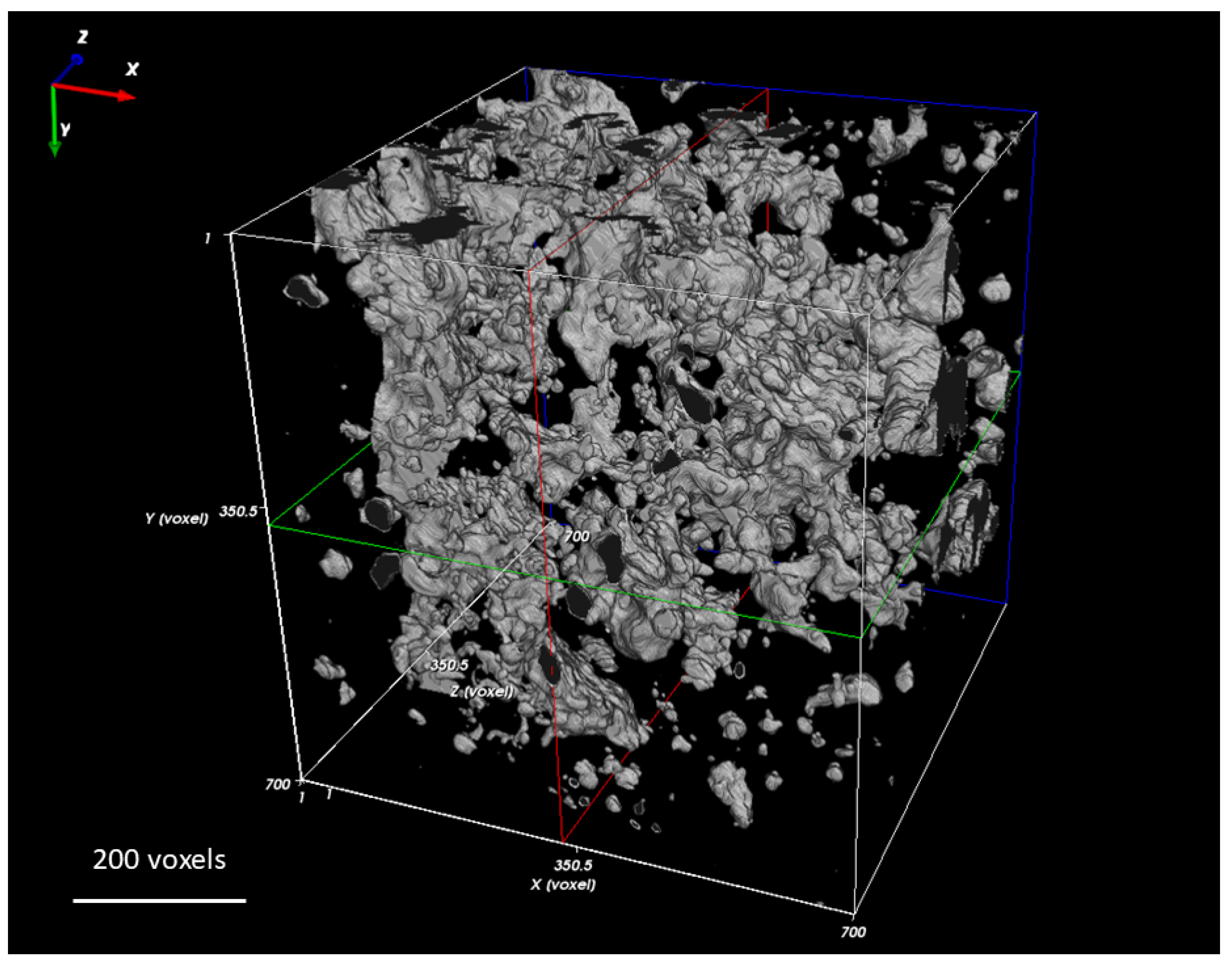
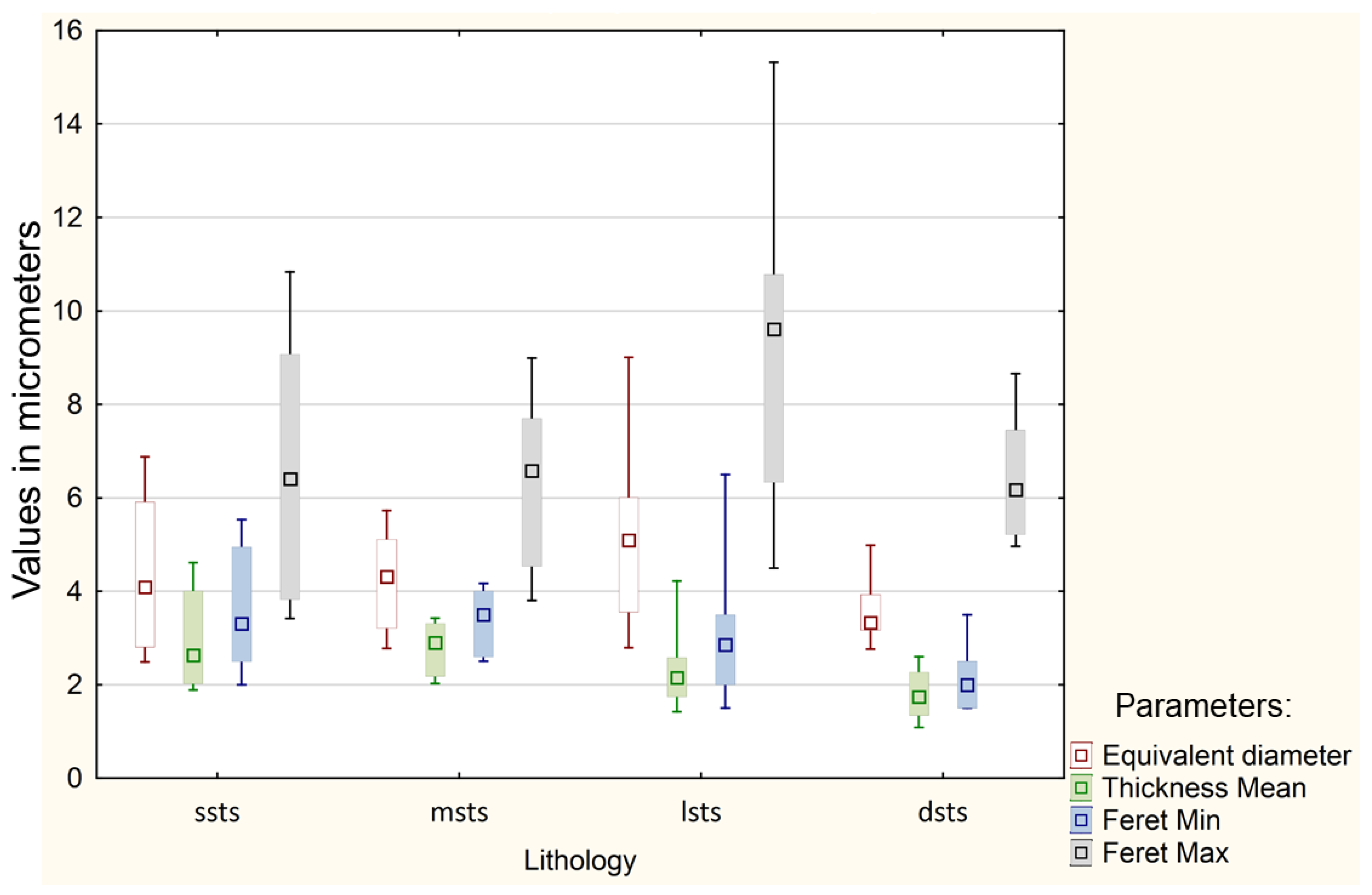
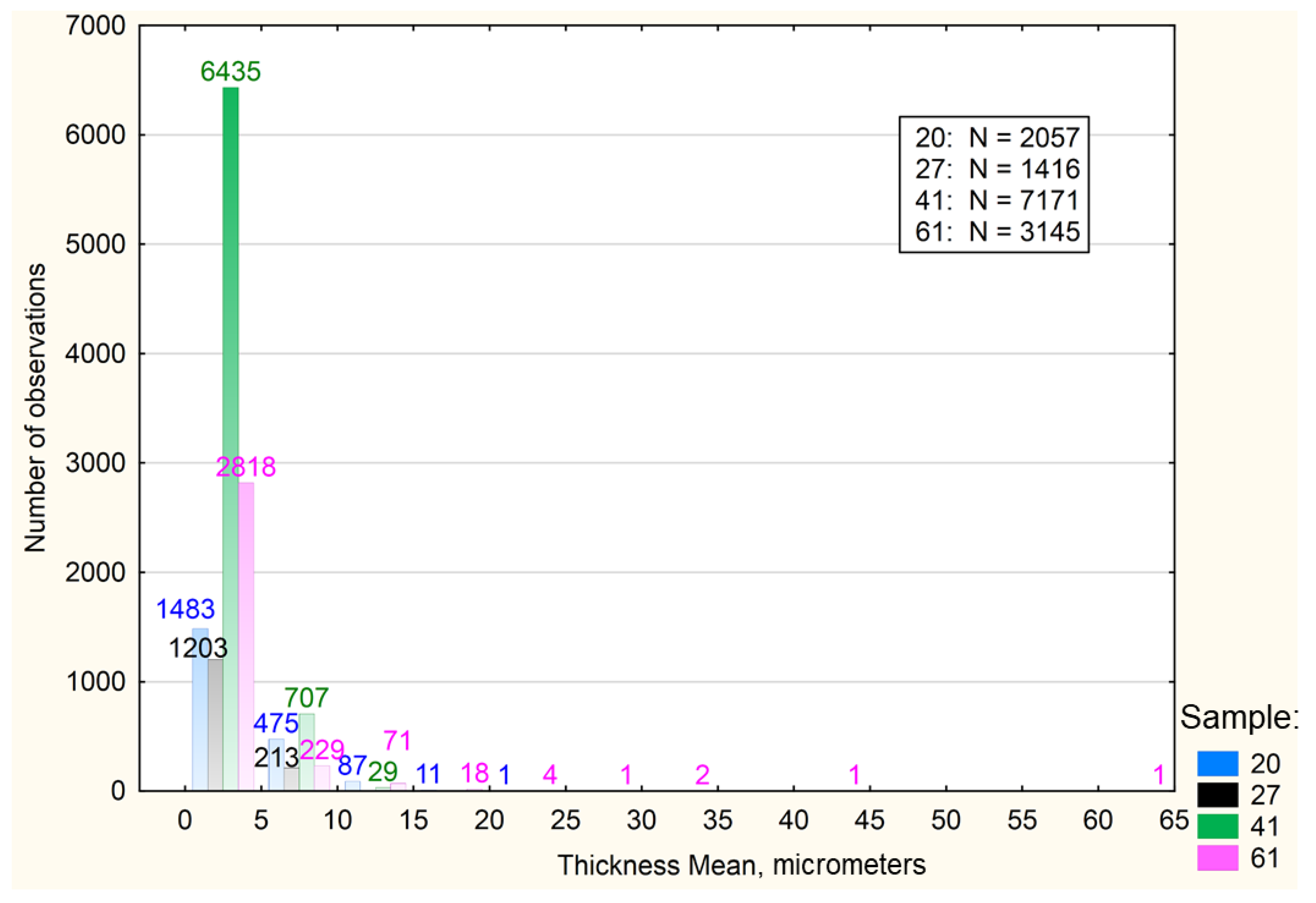
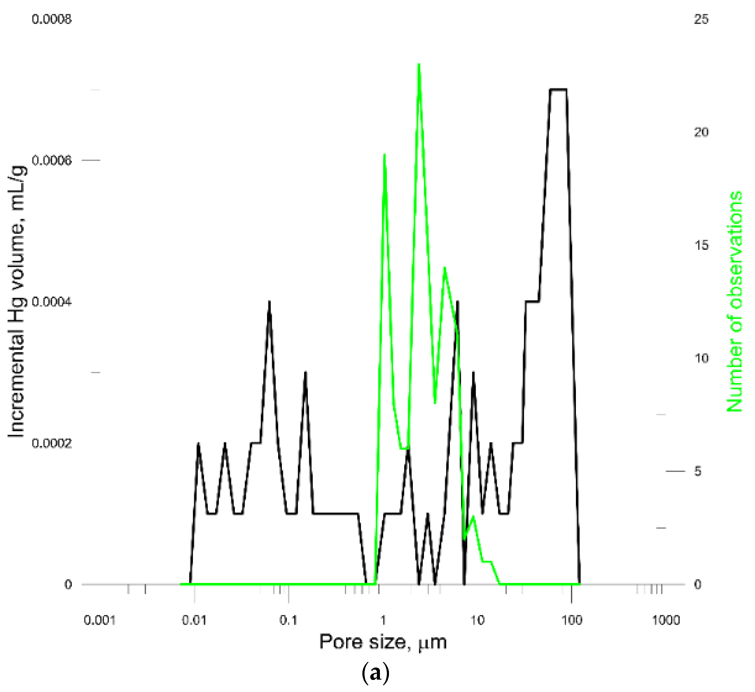



| Element/Process | Description |
|---|---|
| X-ray tube | 57-W, max working voltage 180 kV |
| Detector | Hamamatsu 2300 × 2300 (Ham C 7942CA-02) |
| Voxel size | 0.5 × 0.5 × 0.5 µm3 |
| Reconstruction | Feldkamp algorithm [64] |
| Image processing | Described in [65] |
| Data Set | Parameter |
|---|---|
| The largest object values | Thickness Mean, Volume/Surface Area, Surface Area/Volume, Feret Breadth/Volume, Anisotropy/Thickness Max, Elongation/Thickness Max, Elongation/Thickness Mean |
| Median values | Feret Breadth/Feret Max |
| Maximum values | Thickness Max, Thickness Max/Elongation, Thickness Mean/Elongation, Thickness Mean/Feret Shape |
| Upper quartile values | Flatness, Equivalent Diameter/Feret Max, Thickness Mean/Feret Max, Flatness/Anisotropy, Feret Breadth/Feret Max, I3/I2 |
| Lower quartile values | Feret Max/Equivalent Diameter, Anisotropy/Flatness, Anisotropy/ShapeVA3D, Feret Max/Flatness, Feret Breadth/Flatness, Feret Max/Feret Breadth, I2/I3 |
| Percentile 10 values | Anisotropy, Feret Max/Thickness Max, Feret Max/Thickness Mean, Anisotropy/Flatness, Anisotropy/ShapeVA3D |
| Percentile 90 values | Flatness, Sphericity, Thickness Max/Thickness StD, Thickness Mean/Thickness StD, Elongation/Anisotropy, Flatness/Anisotropy, ShapeVA3D/Anisotropy, Flatness/Feret Max, Flatness/Feret Breadth, Flatness/Feret Shape, I3/I2 |
| Standard deviation values | Elongation/Thickness Max, Elongation/Thickness Mean, Thickness StD/Elongation, Thickness StD/Feret Shape, Elongation/Anisotropy, Flatness/Anisotropy, ShapeVA3D/Anisotropy, Flatness/Feret Shape |
| Type of Data Set | Basic Parameters and Standardized Partial Regression Coefficients | R MLR |
|---|---|---|
| Lower quartile | Equivalent Diameter, −2.0; Thickness Mean, 1.99; Anisotropy, −1.5; Elongation, −1.9; Thickness StD, 0.34; ShapeVA3D, −0.44 | 0.76 |
| Upper quartile | Flatness, 0.73; Feret Min, −2.0; Feret Max, 2.23; Feret Shape, −0.70; Elongation, −0.43; ShapeVA3D, 0.28 | 0.67 |
| Percentile 10th | Thickness Mean, 0.47; Anisotropy, −0.83; Elongation, −1.20; Flatness, −0.03; Feret Min, 0.48; Feret Max, −0.71 | 0.76 |
| Percentile 90th | Thickness StD, −2.1; Feret Max, −2.6; Feret Breadth, 3.89; Feret Shape, 0.65; I3, 0.18, Sphericity, 0.32 | 0.66 |
| Median | Equivalent Diameter, −1.2; Thickness Mean, 1.44; Flatness, 1.69; I1, −4.4; I2, 4.32; Anisotropy, 1.89 | 0.61 |
| Parameter Description | Symbol | Partial Regression Coefficient b (b0–b6) | Standardized Partial Regression Coefficient b* |
|---|---|---|---|
| Intercept in the Equation (2) | - | 14.38 | − |
| Feret Breadth/Volume (from the largest object data set) | 467.62 | 0.28 | |
| Flatness/Anisotropy (from the upper quartile data set) | −9.01 | −3.73 | |
| Feret Max/Flatness (from the lower quartile data set) | −0.10 | −0.40 | |
| I2/I3 (from the lower quartile data set) | −15.22 | −1.38 | |
| Flatness/Anisotropy (from the 90th percentile data set) | 5.92 | 3.70 | |
| Anisotropy/Flatness (from the 10th percentile data set) | 12.75 | 1.21 |
Publisher’s Note: MDPI stays neutral with regard to jurisdictional claims in published maps and institutional affiliations. |
© 2021 by the authors. Licensee MDPI, Basel, Switzerland. This article is an open access article distributed under the terms and conditions of the Creative Commons Attribution (CC BY) license (https://creativecommons.org/licenses/by/4.0/).
Share and Cite
Krakowska-Madejska, P.; Puskarczyk, E.; Habrat, M.; Madejski, P.; Dohnalik, M.; Jędrychowski, M. Development of a Permeability Formula for Tight and Shale Gas Reservoirs Based on Advanced High-Precision Lab Measurement Techniques. Energies 2021, 14, 2628. https://doi.org/10.3390/en14092628
Krakowska-Madejska P, Puskarczyk E, Habrat M, Madejski P, Dohnalik M, Jędrychowski M. Development of a Permeability Formula for Tight and Shale Gas Reservoirs Based on Advanced High-Precision Lab Measurement Techniques. Energies. 2021; 14(9):2628. https://doi.org/10.3390/en14092628
Chicago/Turabian StyleKrakowska-Madejska, Paulina, Edyta Puskarczyk, Magdalena Habrat, Paweł Madejski, Marek Dohnalik, and Mariusz Jędrychowski. 2021. "Development of a Permeability Formula for Tight and Shale Gas Reservoirs Based on Advanced High-Precision Lab Measurement Techniques" Energies 14, no. 9: 2628. https://doi.org/10.3390/en14092628
APA StyleKrakowska-Madejska, P., Puskarczyk, E., Habrat, M., Madejski, P., Dohnalik, M., & Jędrychowski, M. (2021). Development of a Permeability Formula for Tight and Shale Gas Reservoirs Based on Advanced High-Precision Lab Measurement Techniques. Energies, 14(9), 2628. https://doi.org/10.3390/en14092628


