Modeling of Ethiopian Wind Power Production Using ERA5 Reanalysis Data

Abstract

Ethiopia has huge wind energy potential. In order to be able to simulate the power system operation, hourly time series of wind power is needed. These can be obtained from ERA5 data but first a realistic model is needed. Therefore, in this paper ERA5 reanalysis data were used to model wind power production at two topographically different and distant regions of Ethiopian wind farms—Adama II and Ashegoda. Wind speed was extracted from the ERA5 nearest grid point, bi-linearly interpolated to farms location and statistically down-scaled to increase its resolution at the site. Finally, the speed is extrapolated to hub-height of turbine and converted to power through farm specific power curve to compare with actual data for validation. The results from the model and historical data of wind farms are compared using performance error metrics like hourly mean absolute error (MAE) and hourly root mean square error (RMSE). When comparing with data from Ethiopian Electric Power (EEP), we found hourly MAE and RMSE of 2.5% and 4.54% for Adama II and 2.32% and 5.29% for Ashegoda wind farms respectively, demonstrating a good correlation between the measured and our simulation model result. Thus, this model can be extended to other parts of the country to forecast future wind power production, as well as to indicate simulation of wind power production potential for planning and policy applications using ERA5 reanalysis data. To the best of our knowledge, such modeling of wind power production using reanalysis data has not yet been tried and no researcher has validated generation output against measurement in the country.

1. Introduction

The pressure of human life on the world over the past several years, and especially the industrial revolution, resulted in a consistent increase in greenhouse gas production (mainly CO₂) caused by the burning of fossil fuels and brings global warming. This occurred due to deforestation, urbanization, agricultural expansion, transportation, the manufacturing industry and fossil fuel based thermal power plants [1,2,3]. The relationship between food, energy and water is highly increasing and has an effect on climate change, which highly affects emissions unless properly managed. Thus, issues related to water, production of and universal access to energy, as well as food production and their frequent lack, are contemporary problems of the population occurring in many countries [3] and, due to a number of variables, such as population growth, urbanization, rising incomes, the resulting changes in consumption patterns and climate change, the situation in these three sectors is systematically changing. For example, in order to produce food, energy is needed and to get electricity, water is needed.

A report by the United States Environmental Protection Agency indicated that electricity and heat production make up a high share of total CO₂ emissions, which is around 25% [4]. Today, primary energy sources are non-renewable fossil fuels (coal, oil, etc.). The global reserves of these fuels are continually diminishing with increasing consumption and may not be available for future generations. For sustainable and clean energy sources, the world is focusing on renewable energy resources, which accounts for only 13.5% of the global energy mix at the moment [5].

In recent decades, electricity costs from all commercially available renewable power generation technologies are declining towards the cost of the well-developed hydroelectric generation cost. Report [6] indicated that the global average price of electricity was USD 0.05 per kilowatt-hour (kWh) from hydro power projects while it was USD 0.06/kWh for onshore wind and 0.07/kWh for bio-energy and geothermal projects.

Therefore, global warming, fossil fuel depletion and the attractive declining cost of renewable energy have initiated global interest in the mass production of electric energy from renewable energy sources. These days, wind energy technology in particular has developed such that wind generated electric energy has reached more than 5.1% of the total electric energy generation worldwide [5]. Thus, wind power production is continually increasing globally and has become a major challenge in the operation of the grid.

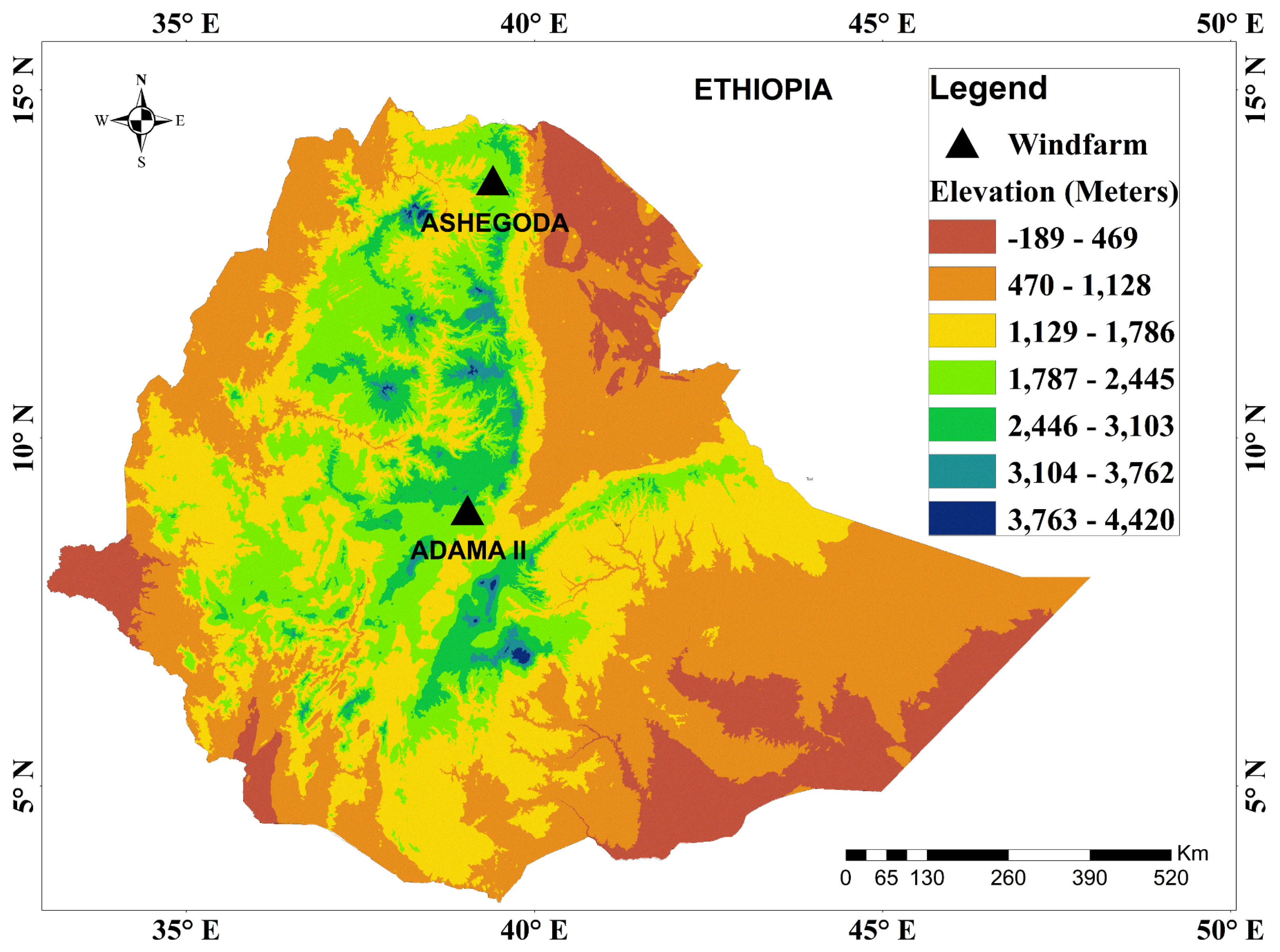
Ethiopia is a big and landlocked country in the Horn of Africa (38.5${}^{\circ }$ E, 9${}^{\circ }$ N) see Figure 1. The topography of the country is a bit complex, as can be seen from Figure 1. Its electric power mix is 94.7% from hydro power, less than 5.2% from wind power [7] and the remaining is from geothermal and diesel. Since hydro power is prone to climate conditions and therefore, during drought seasons, the country has suffered electric energy shortages and is forced to be under scheduled load shading, which is the motivation to expand wind energy as the next alternative for upcoming time. The same problem happened in Poland, when due to drought, the country had to shut down five hydropower plants [3].

Preliminary analysis [8] has shown a very large potential of wind power in Ethiopia, which is 1350 GW at a wind speed of more than 7 m/s, see

Table 1. Information on existing potential resources of each type and how much has been exploited so far.

Resources	Unit	Exploitable Potential	Exploited Amount
Hydropower	GW	45	4.2
Wind	GW	1350	0.324
Solar/day	kWh/m2	4–6	0
Geothermal	GW	67	0.0073
Wood	Million tons	1120	560
Agricultural	Million tons	15–20	6
Coal	Million tons	300	0
Natural Gas	Billion tons	116	0
Oil crude	Million tons	253	0

. But, the installed capacity is only 324 MW which is 5.2% of the total electric power installed capacity. There are a couple of literature studies that deal with the wind energy potential assessment in Ethiopia for different sites [9,10,11]. All the studies were carried out using the data collected from masts installed in the country through the National Meteorological Services Agency (NMSA).

Thus, the country has a plan to install more wind farms and to increase the energy share from wind source. However, wind power is an intermittent and variable power source which makes production planning and system operation more difficult [12,13,14]. The variability of renewable energy sources is indispensable to study, since it affects balancing power costs, required reinforcement in transmission capacity, CO₂ emissions and electricity prices [12,14,15]. Thus, in order to integrate huge amounts of wind power to the grid and to make the correct decisions about when and where to install wind farms, a convincing model of hourly wind power production is indispensable [15,16].

The modeling of wind power production can be done using either statistical [17,18,19] or physical methods [15,20]. Physical models can be implemented based on meteorological measurements or on meteorological models. Physical models simply consider physical features, such as topography, surface roughness, area temperature and pressure, to estimate perfectly the wind field, whereas statistical methods use statistical models in order to create the relationship between power and additional variables and also their measured and predicted values [18]. The meteorological models could either be used directly or use statistical or dynamic downscaling to increase its resolution [15].

Meteorological measurements could be obtained from sites using installed masts. However, this method is the most expensive, time consuming and often incomplete. The mast may not be sited at a relevant wind generation site and at the right altitude above the ground (usually 10 m), which may distort the generation profile [16]. This problem is more pronounced for developing countries like Ethiopia, where resources are highly limited in order to collect wind speed and direction at the required height and site.

On the other hand, meteorological models have available data that is complete with respect to time, space and collected at a high height. One of the meteorological models available is reanalysis data. A reanalyses dataset is the result of binding a state-of-the-knowledge numerical model with the assimilation of past observations from several sources to produce consistent data for a long record of time [16]. It is an essential resource in different research disciplines to investigate the past atmospheric conditions [21,22,23,24,25,26]. Some examples of reanalysis data are MERRA-2 from NASA, ERA5 and ERA-Interim from ECMWF, and so forth. The characteristics of each reanalysis dataset have been shown in

Table 2. Information on freely available reanalyses data. For reference, one degree corresponds to 111 km at the equator (but less in the longitudinal direction closer to the poles). Spatial and temporal resolutions are given for publicly available data. Time coverage and height at which data have been collected is also shown.

Name of Dataset	Spatial Resolution	Temporal Resolution	Time Coverage	Height
ERA5	0.28° × 0.28°	1 h	1979–present	100 m
MERRA-2	0.5° × 0.625°	6 h	1957–present	50 m
MERRA	1/2° × 2/3°	1 h	1979–2016	50 m
ERA-Interim	79 km	6 h	1979–2019	50 m
ERA-40	1.125°	6 h	1957–2002	50 m

[15,24,27,28,29,30,31,32,33,34].

However, as can be seen from Table 2, because of its low resolution (especially spatial) reanalysis data do not consider the local effect of site and therefore, it is not possible to directly utilize for investment decisions and planning unless they are properly processed especially for onshore wind power production [15]. The study done in [16] has explored the role of reanalysis data in simulating regional wind generation variability. Another study done by [15] has used MERRA reanalysis data to model Swedish wind power production by applying different parameters and bias correction to minimize the uncertainty. Reference [35] simulated European wind power generation, applying statistical downscaling to reanalysis data and the paper revealed the importance of statistical downscaling to extract wind speed from the reanalysis data to increase its resolution. The basic steps of the model used here are:

• Extract ERA5 wind speed hourly time series, which has a resolution specified at Table 2 and collect wind farm information like installed capacity and coordinates (location). This concept is described in Section 2.1.
• Bilinearly (horizontal) interpolating ERA5 hourly wind speed from geographical grid points to real wind farms location as described in Section 2.2.2.
• Spatial statistically downscaling of the bilinearly interpolated ERA5 wind speed to increase its resolution as described in Section 2.2.1.
• Calculate true wind speed at farm’s hub height from the downscaled ERA5 hourly wind speed using power law as described in Section 2.2.2.
• Calculate hourly wind energy for each farm from true wind speed using farm’s turbine specific power curve by considering losses like wake loss, internal losses and external losses. It is described in Section 2.2.3.
• Use bias correction to consider the underlying meteorological model uncertainty based on observed bias in wind energy calculated at step 5 compared to the historical energy collected from farm.The idea here is to have the same simulated result with the actual data by correcting the error and uncertainty from the meteorological model. It is described in Section 2.2.3.

The main purpose of this paper is to model wind power production using the ERA5 dataset and to evaluate the application of this dataset for the Ethiopia wind power sector. The model is expected to consider the wind farms, wake losses and systematic error in the underlaying meteorological model. Data from 2016 were used for model training and from 2017 for model evaluation. Section 2 describes the methods used and Section 3 describes the results and discussion. Finally, Section 4 presents the conclusion and suggestions for future work.

2. Methods

In this section, the methods to be used for the modeling of wind power production using the ERA5 dataset are presented. It starts with briefly describing study area, data collection and discusses methods used for the modeling of wind power production.

The workflow of the paper is given in Figure 2 and it indicates that the paper starts with the extraction of wind speed from a reanalysis dataset called ERA5 and the application of horizontal interpolation—known as bilinear interpolation—of wind speed to farm location. After interpolating, spatial statistical downscaling could be applied to increase the resolution of the reanalysis wind speed and finally extrapolating it to turbine hub-height in order to obtain real wind speed at the site.

After getting the wind speed at the required hub-height, it is then possible to convert to power using a farm-specific power curve by applying wake loss in the farm, and finally the work will be concluded by comparing the model result with measurements from the farm.

2.1. Study Area and Data

The specific study was carried out in Ethiopia (see Figure 1), particularly at Adama II wind farm located at (8.5${}^{\circ }$ N & 39.2${}^{\circ }$ E) and Ashegoda wind farm located at (13.49${}^{\circ }$ N & 39.68${}^{\circ }$ E). Two-year (from January 2016 to December 2017) wind speed data were obtained from the European Centre for Medium range Weather Forecasting (ECMWF) and power measurements were collected from Ethiopian Electric Power (EEP). Both data sources will be discussed in the subsequent sections.

2.1.1. ERA5

Reanalysis is the process in which constant data assimilation system is used to give a consistent reprocessing of meteorological observations, typically covering an extended segment of the historical data record [36]. There are many powerful reanalysis datasets commonly used for modeling wind power production like MERRA (Modern Era Retrospective Analysis for Research and Applications) from NASA, ERA5 from ECMWF, etc.

ERA5 is the latest of all and selected for this work because of its high resolution compared to the others as shown in Table 2. It is available in the Climate Data Store on regular latitude-longitude grids at 0.28${}^{\circ }$× 0.28${}^{\circ }$ (31 km) spatial and one-hour temporal resolution. ERA5 covers the period from 1979 to present and wind speed data is freely available at a height of 100 m, that is, relevant for modern wind turbines (WTs). The horizontal resolution is around 31 km, which is better than any reanalysis data [29,36]. Due to the limited spatial resolution there is uncertainty in ERA5 reanalysis data though it is better than forecast.

2.1.2. Wind Power Measurement Data

Historical generation output data of wind farms for the stated period were obtained from Ethiopian Electric Power (EEP). In order to successfully model the generation and evaluate its performance, the following data have been collected.

• Location (coordinates) and installed capacity of the farms.
• Hourly mean measurements of wind farms generation.

The measurement data from EEP has many errors, for example negative and sometimes more than rated power are recorded and those parts of the data were removed first. Another problem is, most of the time the measurement is zero. This may be due to turbine downtime or again due to measurement error compared to the model output. Those parts of the data were also removed. The turbine type, turbine rating, installed capacity and number of turbines per farm are given in

Table 3. Information on wind farms turbine type, rating and installed capacity.

Wind-Farm Name	Turbine Type	Power Rating (MW)	Installed Capacity (MW)	Number of Turbine (m)	Hub-Height (m)
Ashegoda	Ecotecnia 74	1.67	120	84	70
Adama II	Sany SE7715	1.5	153	102	80

.

Next, for comparison between measurement and model, the capacity factor of the power time series is calculated for each farm using Equation (1).

$$CF=\frac{P_{MW}}{P_{inst}},$$

(1)

where: CF is capacity factor, $P_{MW}$ is the actual generation and $P_{inst}$ is the installed capacity.

2.2. Model of Wind Power Production

The general approach to converting wind speed into power consists of converting wind speed data from meteorological models or observations using a farm specific power curve. The power curve provides the value of an electrical power output as a function of wind speed at turbine hub height. The conversion of wind speed time series to its equivalent power time series using reanalysis data has been done by many researchers since the release of the data. However, the level of complexity of conversion differs from one researcher to another in the possible use of the parameters that are to be optimised. The parameters used in this paper are listed in

Table 4. Parameters used in the model.

Parameter Name	Range	Description
$Losse{s}_S$	[0.0, 0.25]	Loss used when calculating scaling constant of wind speed and it is discussed in Section 2.2.2
$PLos{s}_{int}$	[0.00, 0.30] × 12	Internal power losses in the incoming wind speed for each wind sector and it is discussed in Section 2.2.3
Bias correction	12 × 24 matrix	A matrix correcting for seasonal and diurnal bias for each farms and discussed in Section 2.2.3

.

Thus, in this paper, the method for modeling hourly wind power production starts with a mathematical calculation to determine wind speed at the required site and hub height from reanalysis data and converts the calculated wind speed to power through the farm specific power curve. Finally, it discusses the loss to be considered in the farm and systematic bias in the meteorological model.

2.2.1. Spatial Statistical Downscaling of ERA5 Wind Speed

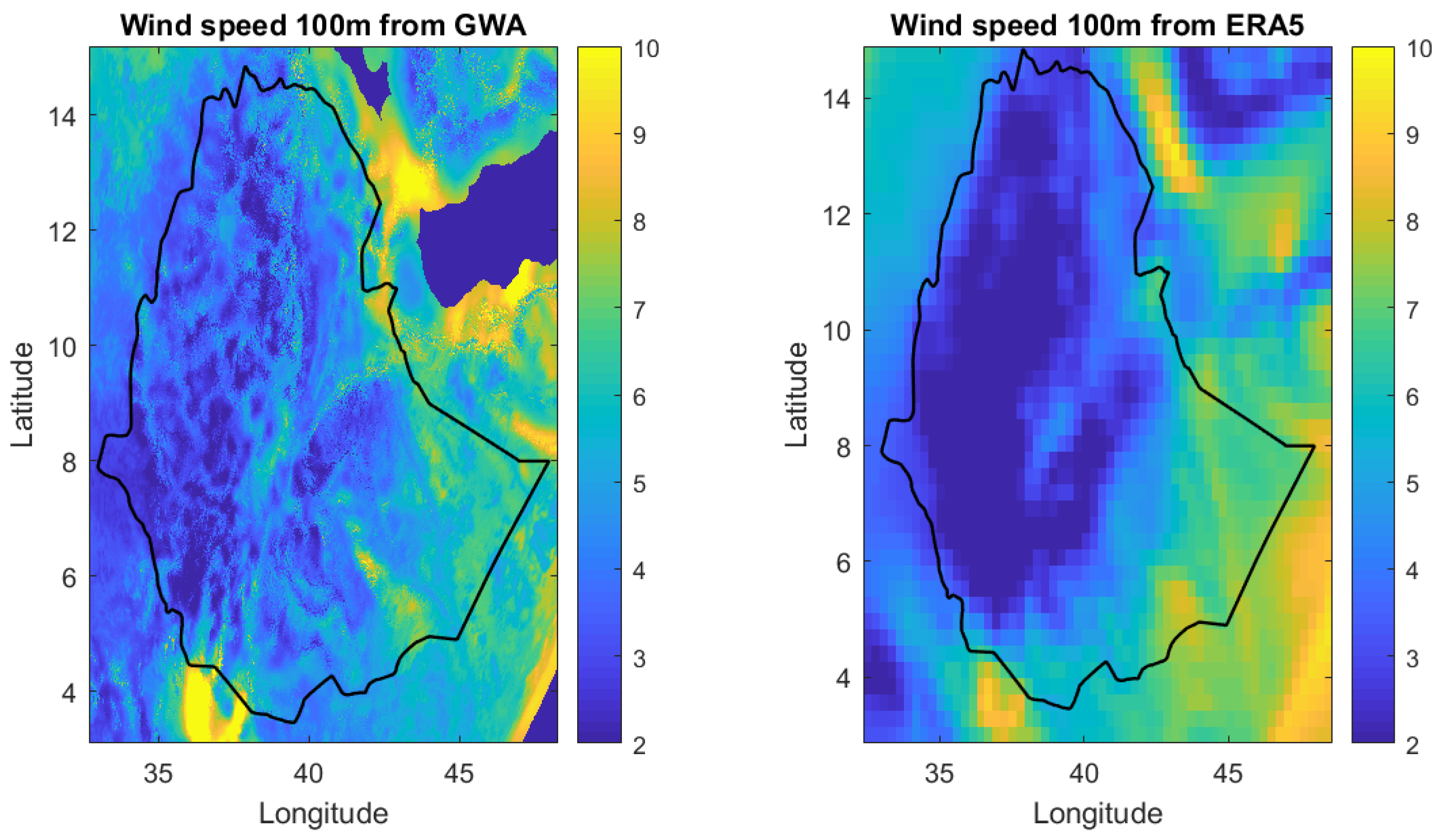
Although ERA5 wind speed is taken from reanalysis and consequently should have lower errors compared to forecasts, there are still uncertainties partly due to the limited spatial resolution as well as uncertainties in the meteorological model itself. The spatial resolutions of ERA5 and GWA are illustrated qualitatively in Figure 3 and that the colors represent different ranges of mean wind speeds of the site at 100 m height. Thus, as can be seen from the figure, GWA gives a more compact pattern than ERA5. This is due to the low spatial resolution of ERA5 dataset.

In order to increase the resolution and to reduce systematic bias of this reanalysis data, different researchers have followed different methods. Some of them used the bias correction method [15,37,38] and others have used the spatial statistical downscaling method [35,39].

In this paper, the statistical downscaling method is applied to ERA5 data to increase the spatial resolution of wind speed to consider the local effect around wind farms. The spatial statistical downscaling technique is applied to reanalysis wind speed data [35] by using the Global Wind Atlas (GWA) data, which considers local orography and surface roughness features at 250 × 250 m spatial resolution.

Each value of low resolution wind speed arising from the ERA5 hourly time series is then associated to the value of high resolution wind speed, leading to equal values of cumulative distribution function as shown in Equation (4) [35]. The approach has been applied to hourly wind speed at stated wind farms in order to capture the local effect. Weibull parameters, shape factor (k) and scale factor (c) of reanalysis data are estimated using empirical methods in order to best fit wind speed distribution of the site using Equations (2) and (3) and the micro-scale values of the same parameters are obtained from a global wind atlas.

$$k={\left(\frac{\delta }{V}\right)}^{-1.086}$$

(2)

$$c=\frac{V}{gamma\left(1+\frac{1}{k}\right)}$$

(3)

$$F_{HR}\left(v_{HR}\right)=F_{LR}\left(v_{LR}\right)$$

(4)

$$1-e^{-{\left(\frac{v_{HR}}{c_{HR}}\right)}^{k_{HR}}}=1-e^{-{\left(\frac{v_{LR}}{c_{LR}}\right)}^{k_{LR}}},$$

(5)

where:

• k is the shape factor of of Weibull distribution,
• c is the scale factor of Weibull distribution,
• V is the mean wind speed,
• $\delta$ is the standard deviation of the wind speed,
• $F_{LR}$ is the cumulative distribution function of low resolution,
• $F_{HR}$ is the cumulative distribution function of high resolution,
• $v_{LR}$ is the low resolution wind speed time series &
• $v_{HR}$ is the high resolution wind speed time series to be calculated.

Solving $v_{HR}$ from Equation (5), it becomes:

$$v_{HR}=c_{HR}{\left(\frac{v_{LR}}{c_{LR}}\right)}^{\frac{k_{LR}}{k_{HR}}}.$$

(6)

2.2.2. Interpolation and Extrapolation

The statistically downscaled hourly wind speed has to be bilinearly interpolated to the wind farm location and vertically extrapolated to hub height. Horizontal interpolation is performed with the bilinear method and vertical extrapolation is performed with power law and is given by Equation (7).

$$v_{HRtur}=v_{HR100\mathrm{m}}{\left(\frac{h_{tur}}{h_{100\mathrm{m}}}\right)}^{\alpha },$$

(7)

where:

• $v_{HRtur}$ is wind speed at turbine hub-height,
• $v_{HR100\mathrm{m}}$ is ERA5 wind speed at 100 m,
• $h_{tur}$ is turbine hub-height,
• $h_{100\mathrm{m}}$ is the height of ERA5 wind speed and
• $\alpha$ is the shear exponent.

The shear exponent $\alpha$ was calculated from the two heights of the global wind atlas (between 100 and 50 m) and is given by Equation (8).

$$\alpha =\frac{ln\left(\frac{v_{100\mathrm{m}}}{v_{50\mathrm{m}}}\right)}{ln\left(\frac{100\mathrm{m}}{50\mathrm{m}}\right)}.$$

(8)

The shear exponent is assumed to be constant but mean annual energy production (AEP) from reanalysis must be equal to the measurement. In order to achieve this equality requirement, Equation (7) must be multiplied with a constant. Losses in the calculation of AEP are controlled by the parameter $Losse{s}_S$.

2.2.3. Power Curve and Output Power

The power curve from the manufacturer relates wind power to its corresponding wind speed. The power curve used in this paper is farm-specific and the most important factor for the shape of the curve is the ratio of rated power to rotor area or specific power of the turbine $\left(P_A\right)$. The best way to consider the wake effects in the model is to transform the power curves into functions of power in the incoming wind $(P_u$, measured in watts per square metre swept rotor area). Thus, the wind turbine output power is a function of power in the incoming wind $(P_u$) and $P_A$. The relationship is given by Equation (9).

$$P_{tur}=f(P_u,P_A).$$

(9)

In a wind farm there are many kind of losses like wakes effect, blade degradation losses, high wind hysteresis and losses in the transformer and transmission line that could have their own impacton the power to be produced and transmitted to the consumer. The most significant loss to be considered in wind farm is wake effect from upstream turbines. There are many methods used to represent those losses [40,41], including the Katic/Jensen model given by Equation (10).

$$V=U\left(1-\frac{1-\sqrt{1-C_t}}{{(1+2k\frac{X}{D})}^2}\right),$$

(10)

where $C_t$ is the thrust coefficient, V and U are affected and unaffected wind speeds, k is the wake decay constant, X is distance between turbines and D is the diameter of turbine. Due to the fact that the thrust coefficient is higher for low wind speeds, the reduction of wind speed using Equation (10) is also higher in low winds. Because of the nonlinear shape of the power curve, the losses will be zero for unaffected winds below cut-in, increasing to peak in the steepest part of the power curve and then again decrease towards zero for unaffected wind speeds a small above rated. Almost similar shape of wind speed dependent losses could be obtained by reducing the incoming wind energy with a fixed amount (controlled by $Plos{s}_{int})$ in Equation (11) [15].

From the relationship between the turbine output power and power in the incoming wind speed, one can assume two different power losses as loss in the wind due to wake effect and transmission line loss. Thus, the power at the point of common coupling or at the grid can be formulated using Equation (11).

$$P_{pcc}=(1-Plos{s}_{tr})f((1-Plos{s}_{int})\frac{1}{2}\rho u^3,P_A),$$

(11)

where:

• $P_{tur}$ is output power of turbine,
• $P_{pcc}$ is power at the point of common coupling of the grid and
• $\rho$ is air density which is constant (1.225 kg/m³).

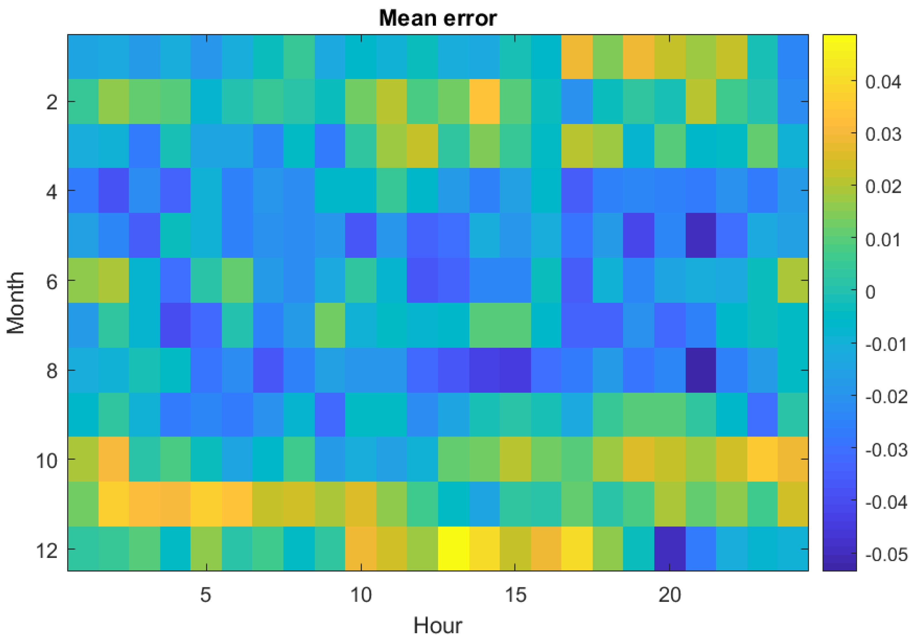
The meteorological model bias correction is performed to consider the seasonal and diurnal bias of reanalysis uncertainty [42]. It is motivated due to an observed ERA5 systematic error depending on month of year and time of the day (see Figure 4). As can be seen from the figure, this error is a function of the month of a year and the hour of a day. These observed errors could be due to the inability of ERA5 to correctly capture the seasonal and diurnal dependence of the wind speed and wind shear.

2.2.4. Performance Metrics

There are several statistical performance error metrics that can be used as appropriate measures of performance for any model. Hourly root mean squared error (RMSE) and hourly mean absolute error (MAE) are used in this paper because of their wide application [43]. Thus, the mathematical expression of the two performance metrics are given by Equations (12) and (13).

$$MAE=\frac{1}{n}\sum _{t=1}^n\left(\left|P_{mt}-P_t\right|\right)$$

(12)

$$RMSE=\sqrt{\frac{1}{n}\sum _{t=1}^n{\left(P_{mt}-P_t\right)}^2},$$

(13)

where:

• $P_{mt}$ is the measured power at time t,
• $P_t$ is the modeled power at time t and
• n is the total number of time.

2.2.5. Model Optimisation

In order to select the optimum value of the parameter listed in Table 4, it is necessary to use the appropriate optimisation technique. The objective is to minimize the root mean square error (RMSE) which is given by Equation (13). This means that in wind power modeling, the main objective is to have minimum error in hourly energy compared to the hourly measurement. Therefore, the objective function (OF) is formulated and given by Equation (14).

$$OF=min\left(RMSE\right).$$

(14)

A nonlinear matlab built in function “Patternsearch optimisation” technique was chosen to tune the parameters to be optimised.

3. Result and Discussion

3.1. Result

In this section, the results of the study are presented and discussed with reference to the aim of the research objective, which is the modeling of Ethiopian wind power production using ERA5 data. The two aims of the study are to model wind power generation and to validate the result against the measurements. At the same time, the study tried to evaluate the suitability of ERA5 reanalysis data for the simulation of hourly wind power generation. The two topographically different and distant regions of Ethiopian wind farms were selected as the study area to assess the suitability of ERA5 data to the country as the first trial.

Simulated wind power production of hourly time series of one year was validated with historical hourly wind power data provided by the Ethiopian electric power (EEP). The performance error metrics for the respective wind farms are shown in

Table 5. Performance error metric result of the model compared with measurement.

Metrics	Ashegoda	AdamaII
MAE	2.32%	2.5%
RMSE	5.29%	4.54%

. The results are given for two years of modeling period between 1 January 2016 and 30 December 2017 Gregorian calendar (G.C). One year was used for model training and the other one year was used for the validation of the model. All results are given in per unit (p.u.), where one p.u. represents the installed capacity of the respective wind farm. The mean absolute error (MAE) and root mean square error (RMSE) of hourly power become 2.32% and 5.29% for Ashegoda and 2.5% and 4.54% for Adama II, respectively.

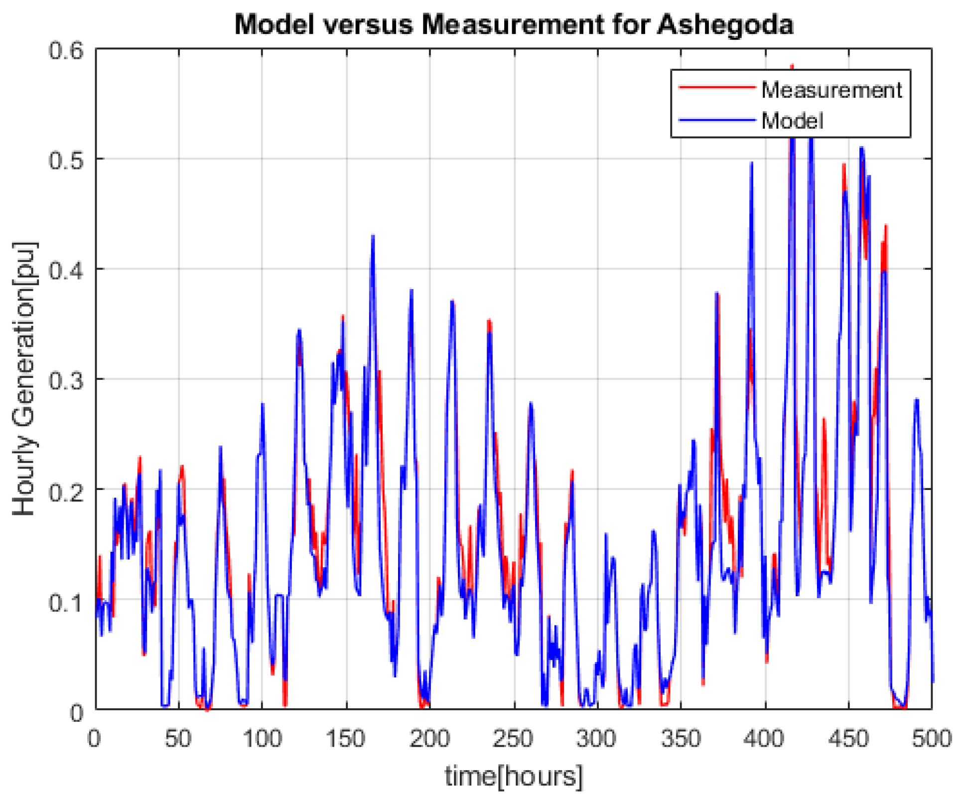
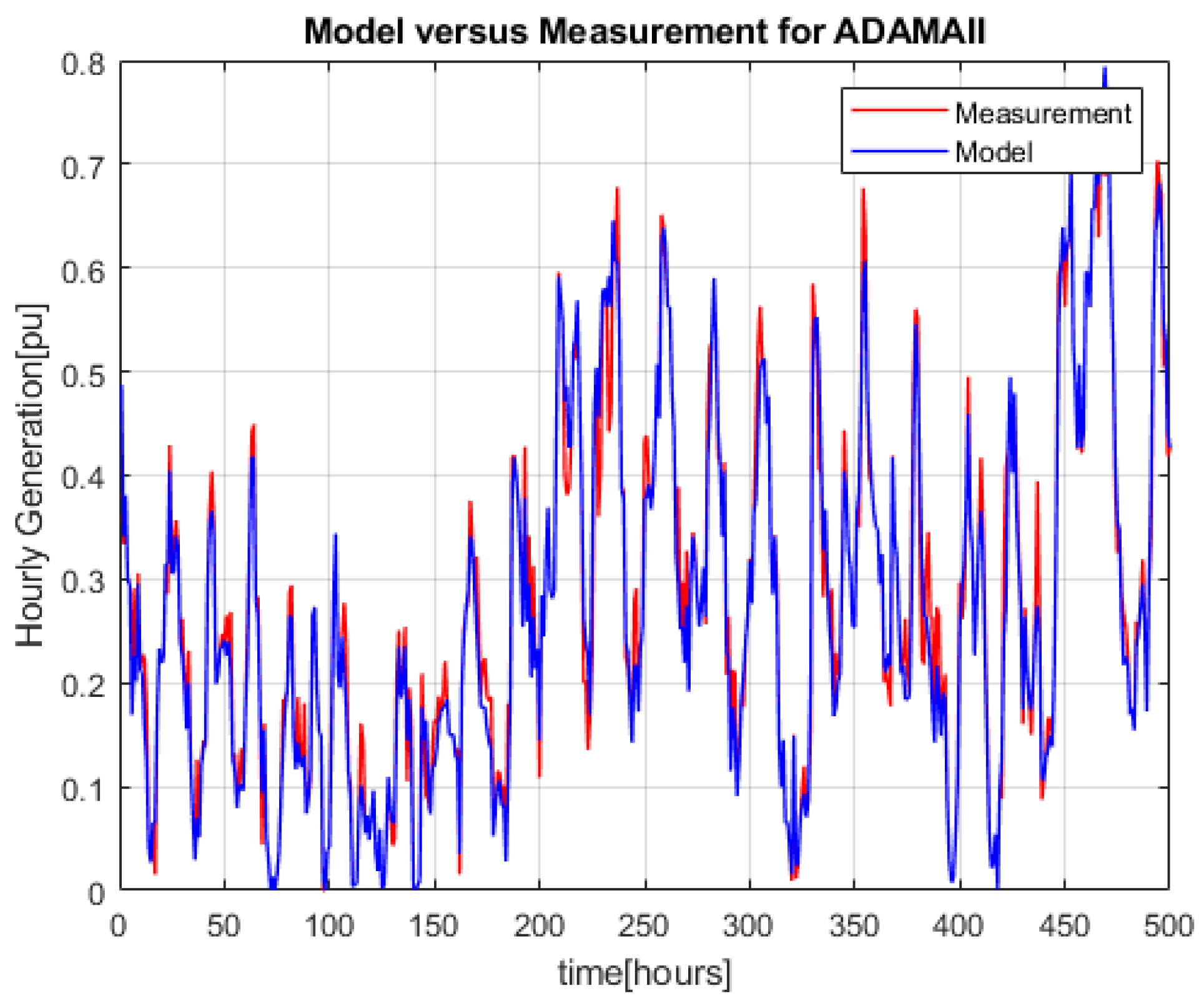
Figure 5 and Figure 6 show model output and measured data for 500 h of Ashegoda and Adama II respectively. The MAE and RMSE for this period is 2.8% and 5.1% for Ashegoda and 3% and 4.8% for Adama II respectively. The result is almost identical to the MAE and RMSE for the full one year of validation period. The figures clearly show that the modeled power can capture the measured hourly power fluctuations.

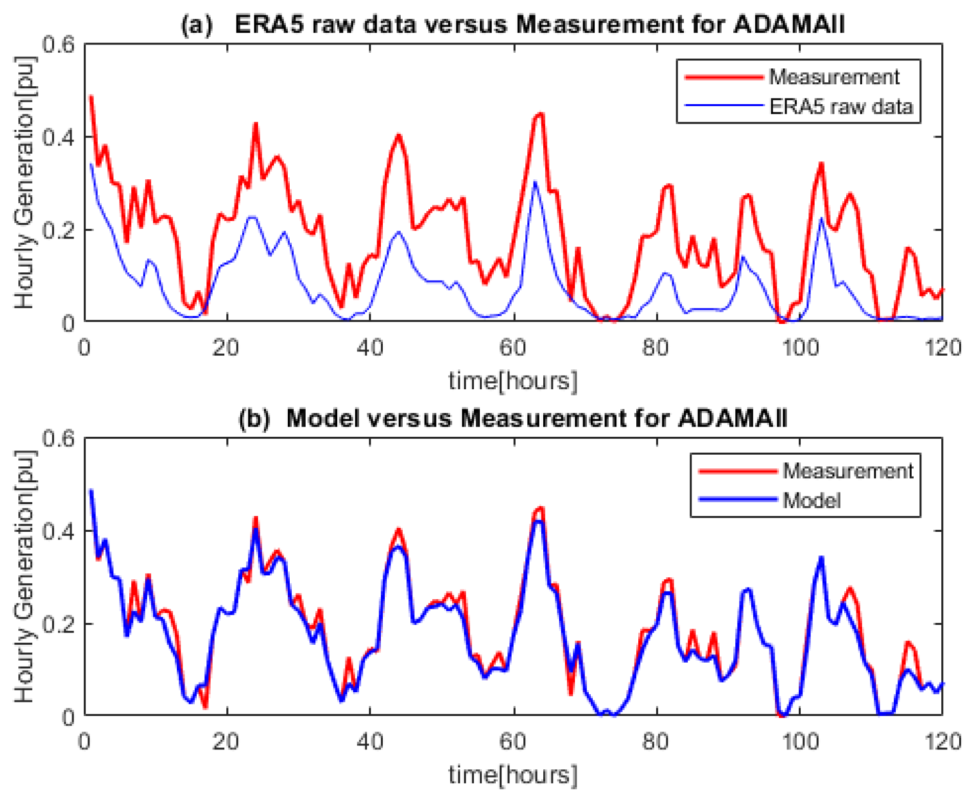
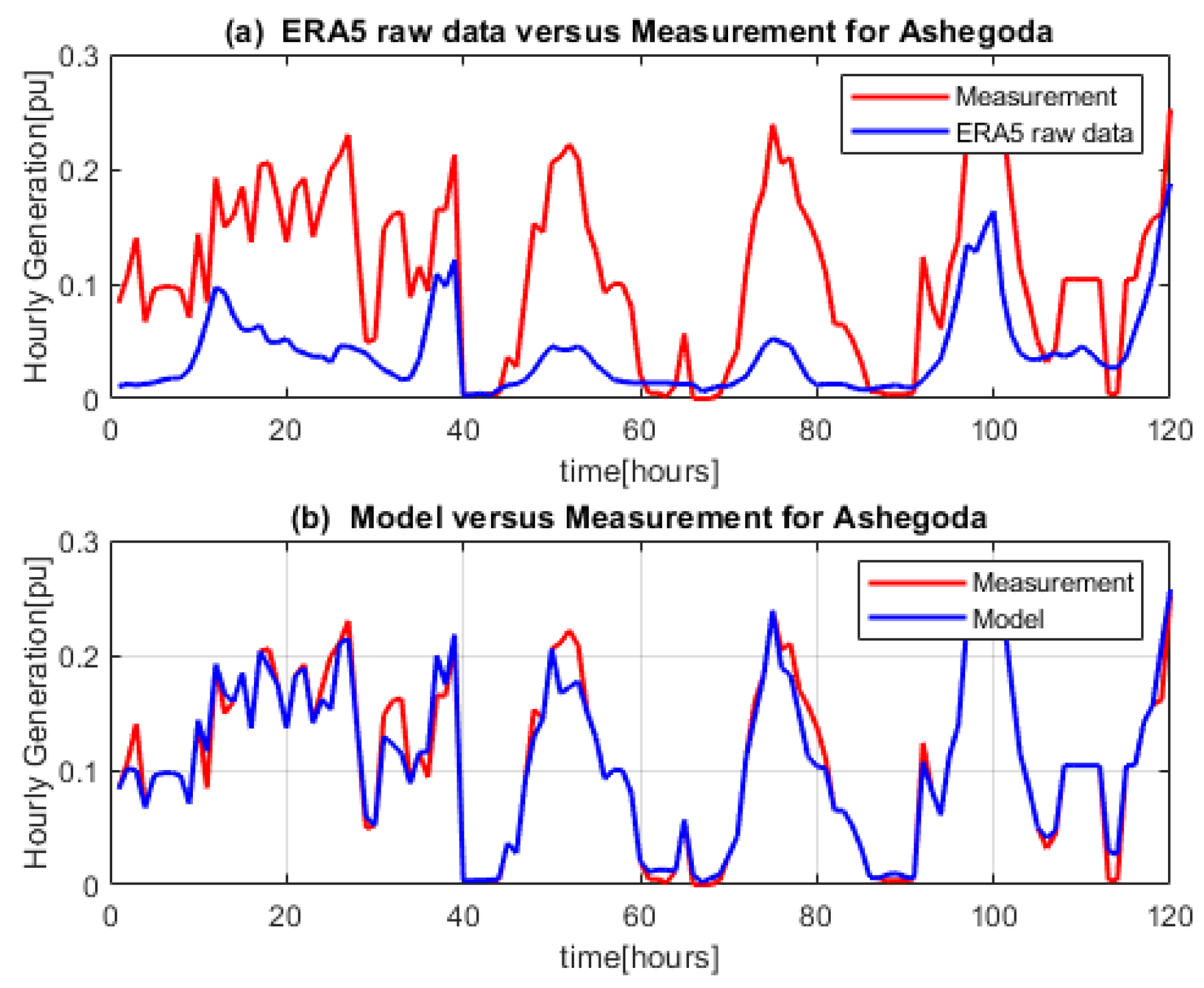
In order to see the characteristics of unmodified ERA5 reanalysis data compared with measurement, the data of both ERA5 and measurement for five days (120 h) is shown in Figure 7 and Figure 8 for both wind farms. From the figures, it can be said that ERA5 raw data more or less follows the measurement hourly pattern. This means that the reanalysis data under consideration captures features of the wind farms power production. In the same figure, the result after the model has also been displayed to show that ERA5 can be used to model wind power production if properly treated.

When comparing this paper with previous work, the error is relatively good, as the work was carried out on individual wind farms, not at the regional or country level, where variation of wind power is smoothed out due to geographic dispersion of plants. J. Olauson and M. Bergkvist [15] modelled Swedish hourly wind power production at regional and country level using the MERRA dataset and the RMS errors became 3.8%. Kubik [16] has modelled for north Ireland using the MERRA dataset and obtained an RMS error of 11.9%, which is higher than the result we obtained in this paper. The reason we obtained a good result here in this paper is the use of statistical spatial downscaling and the use of the ERA5 dataset, which is much better than MERRA data in terms of the space and time resolution.

The above result showed that the proposed model has good agreement with measurements for the two wind farms. If any simple model results with a similar output, it is interesting. Therefore, we set up the following simple model steps for comparison with the proposed model. A simple model is one without statistical downscaling, no wake effect consideration and without bias correction.

• ERA5 hourly wind speed for the 100 m level was bilinearly interpolated to the turbine positions.
• Wind speed extrapolation to turbine hub-height using power law
• The mean wind speed for each site was adjusted in order to give the annual energy production obtained from measurement.
• Hourly power production for each farm was calculated using the farms power curve.

3.2. Effect of Parameters and Discussion of the Result

This section presents the influence of the parameters used on the proposed model and discussion of the result. The result is obtained with the application of spatial statistical downscaling and different parameters to the proposed model. As shown in Table 3, three parameters, including seasonal and diurnal correction, have been considered.

The application of spatial statistical downscaling to reanalysis data using high resolution global wind atlas (GWA) has significantly improved the result for Adama II and moderately for Ashegoda. Without spatial statistical downscaling, the RMSE of the simple model is 11.51% and 10.38% for Adama II and Ashegoda respectively. With spatial statistical downscaling the result is improved by 42.4% for Adama II and by 7% for Ashegoda. This shows that simple model is overestimating the output power than the proposed model. Thus, the downscaling has reduced the objective function value by almost 42.4% and 7% for Adama II and Ashegoda respectively. Therefore, we can conclude that the spatial statistical downscaling in Ethiopian wind power production model is very important parameter and therefore it should be considered while modeling the wind power production by taking the exact coordinate of the site.

Although the wake effect could not be calculated on an individual wind turbine level, the introduction of a global loss factor in the incoming wind power in the wind for each wind sector (bin of 30${}^{\circ }$) has been tried but it did not improve the result for Adama II and it significantly improved it for Ashegoda. The loss of 0–30% was applied and optimised using matlab built-in function “pattern-search” for each different wind sectors. The objective function value was reduced by 17% for Ashegoda. Therefore, for future wind power production simulation, we recommend accounting for some 25% wake effect since the upstream turbine has the mentioned effect.

The introduction of seasonal and diurnal bias correction from the observed bias due to error and uncertainty in reanalysis has significantly improved the objective function value for both wind farms. The value of the objective function without bias correction was 6.63% and 8.16% for Adama II and Ashegoda, respectively. With the bias correction, the RMSE became 4.54% and 5.29% for Adama II and Ashegoda, respectively. This shows that the RMSE value for Adama II and Ashegoda is decreased by 28.05% and 45%, respectively. This indicates that the ERA5 data has bias and it has to be considered while simulating Ethiopian wind power production.

Furthermore, as can be seen from the simulation result of Figure 5 and Figure 6, the model has almost replicated the measurement. From this we can conclude that, using ERA5 reanalysis wind speed data, it is possible to identify the potential areas of wind in different parts of the country before installing wind farms.

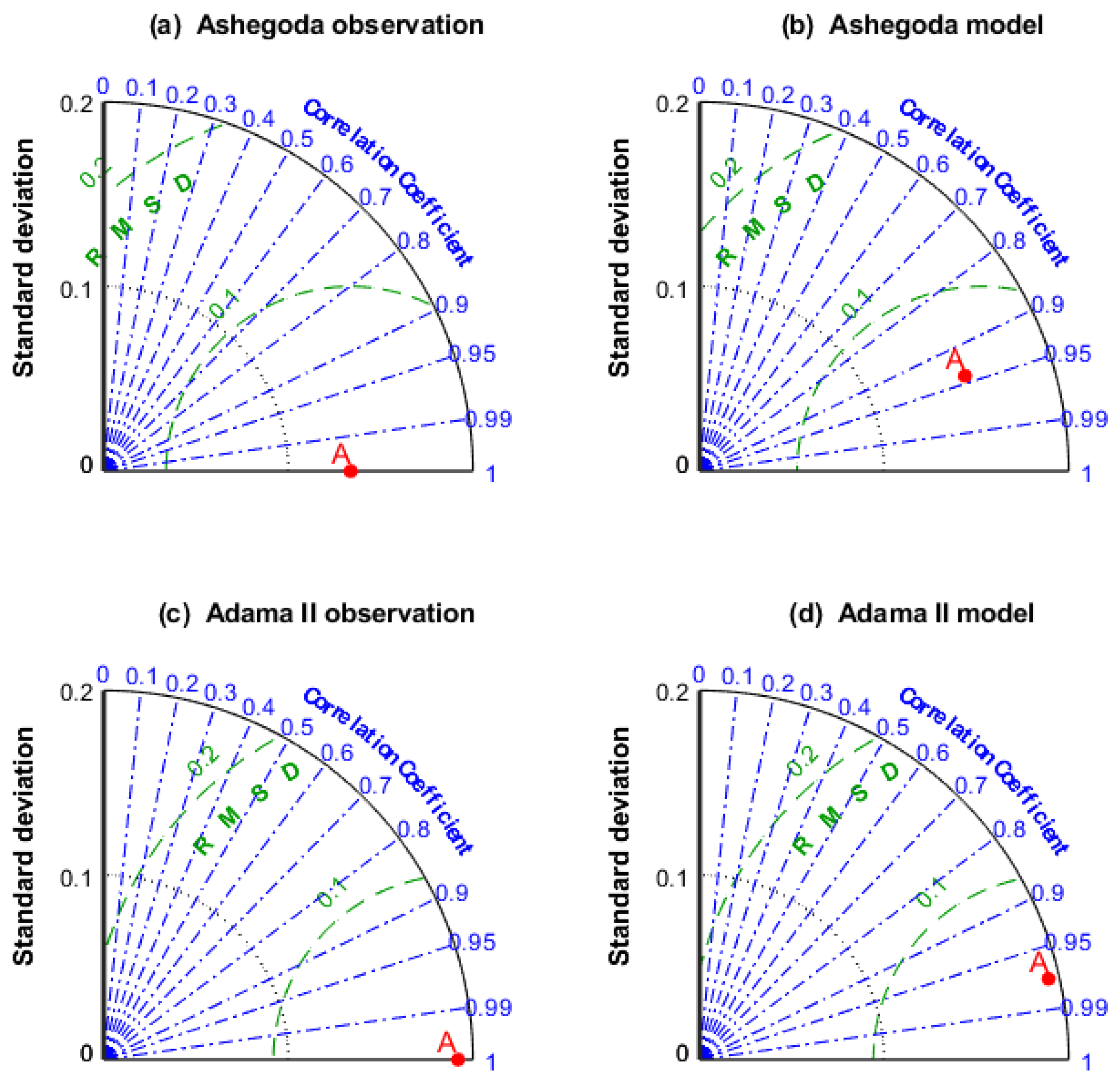
In order to compare the model performance with observation, a Taylor diagram has also been used. This diagram is used to compare the model with observation or measurement in terms of three parameters, standard deviation, root mean square error or deviation (RMSD) and the correlation coefficient. The standard deviation shows how the model varies compared to observation. The RMSD is used to show the model performance and how far the model is from the observation. The last and very interesting variable used to compare the model with the observation is the correlation coefficient. This variable is used to show how well two time series follow each other. Figure 9 shows the combined effect of those three variables (standard deviation, RMSD and correlation coefficient) labelled with a red dot under letter A for observation and the model of each farm. Each farm has the respective plot for observation and model. The observation plot is used as a reference to evaluate the model. Figure 9a,b shows the Taylor diagram of the Ashegoda wind farm for the observation and model, respectively. The three parameter calculation of observation is done with itself and that is why it has a unity correlation coefficient and zero RMSD. Figure 9c,d shows the Taylor diagram of Adama II wind farm for the observation and the model, respectively. As can be seen from the figure, the standard deviation of the model for Adama II and Ashegoda becomes 18.80% and 15.44%, respectively. This value is almost similar to the standard deviation of the measurement, which is 19.19% and 13.38% for AdamaII and Ashegoda, respectively.

In a similar way to the same figure, the RMSD of the model for Adama II and Ashegoda becomes 4.54% and 5.37%, respectively. This shows a small error between the model and the observation and the model has the ability to reproduce the observation.

The correlation coefficient of the model is also shown in the same figure and it becomes 97.47% and 94.03% for Adama II and Ashegoda, respectively. The correlation value is quite high and this means the model time series follows the observation time series. Thus, in general, the three parameter values show that the model performs well and captures the observation time series characteristics.

Thus, in concluding this section, the proposed model has tried to simulate current wind power production and also tried to evaluate the suitability of ERA5 for the Ethiopian wind farm sector. The result has shown us that using ERA5 data, it is possible to model wind power production as well as to identify the potential areas of wind speed of the country. However, the ERA5 data have to be properly processed first to represent the site by appropriate means.

In addition to this, to the best of our knowledge, this is the first trial using reanalysis data to simulate wind power production and validating the result against the measurements in Ethiopia. The result obtained is promising and has shown us that, using reanalysis data, it is possible to model wind power production for any site in the country by properly extracting and processing the wind speed.

4. Conclusions

In this paper, the modeling of wind power production in the case of Ethiopia was carried out and the performance error metrics were evaluated against the measurements. The MAE and RMSE became 3.8% and 4.5%, respectively. The model was created based on ERA5 reanalysis data. Modeling of wind power production using reanalysis data has not yet been tried and no researcher has validated the generation output against the measurements in the country so far. This makes this paper a unique and novel study in Ethiopia.

The work started with extracting wind speed data from the ERA5 meteorological model and statistically downscaled to the site. Since ERA5 does not capture the local effect of the site, statistical downscaling was applied to increase its spatial resolution and brought significant improvement to the output power. Without spatial statistical downscaling, the RMSE of the simple model is 11.51% and 10.38% for Adama II and Ashegoda, respectively. With spatial statistical downscaling, the result was improved by 42.4% for Adama II and by 7% for Ashegoda.

Power loss in the incoming wind speed in each wind sector (bin of 30${}^{\circ }$) as wake loss was considered and it improved the result of the output power. The result showed that this parameter did not improve the result for Adama II and it significantly improved the result for Ashegoda. The objective function value was reduced by 17% for Ashegoda.

The introduction of seasonal and diurnal bias from observed bias also significantly changed the objective function value for both wind farms. The value of objective function without bias correction was 6.63% and 8.16% for Adama II and Ashegoda, respectively. With bias correction, the RMSE became 4.54% and 5.29% for Adama II and Ashegoda, respectively. This shows that the RMSE value for Adama II and Ashegoda decreased by 28.05% and 45%, respectively.

The suitability of ERA5 reanalysis wind speed data as the potential resource to identify the good wind speed areas was also shown. It could be seen from the simulation result that the model almost replicated the measurement when properly treating the ERA5 wind speed.

Thus, the result showed us that ERA5 reanalysis wind speed data can be used to simulate wind power production, as well as to identify the potential areas for other sites of the country, if the wind speed is properly treated.

5. Future Work

The next step will be a study on balancing wind power using any flexible sources in the Ethiopian power system under different penetration levels by creating wind penetration scenarios. The study will include how to smooth the variability of wind power, how to handle the peak load, how to handle the wind and load ramping when the wind penetration level is small and large, respectively.