Forecasting and Modelling the Uncertainty of Low Voltage Network Demand and the Effect of Renewable Energy Sources

Abstract

More and more households are using renewable energy sources, and this will continue as the world moves towards a clean energy future and new patterns in demands for electricity. This creates significant novel challenges for Distribution Network Operators (DNOs) such as volatile net demand behavior and predicting Low Voltage (LV) demand. There is a lack of understanding of modern LV networks’ demand and renewable energy sources behavior. This article starts with an investigation into the unique characteristics of householder demand behavior in Jordan, connected to Photovoltaics (PV) systems. Previous studies have focused mostly on forecasting LV level demand without considering renewable energy sources, disaggregation demand and the weather conditions at the LV level. In this study, we provide detailed LV demand analysis and a variety of forecasting methods in terms of a probabilistic, new optimization learning algorithm called the Golden Ratio Optimization Method (GROM) for an Artificial Neural Network (ANN) model for rolling and point forecasting. Short-term forecasting models have been designed and developed to generate future scenarios for different disaggregation demand levels from households, small cities, net demands and PV system output. The results show that the volatile behavior of LV networks connected to the PV system creates substantial forecasting challenges. The mean absolute percentage error (MAPE) for the ANN-GROM model improved by 41.2% for household demand forecast compared to the traditional ANN model.

1. Introduction

Load forecasting is a significant tool utilized to evaluate power consumption, or future energy [1,2]. One of the fundamentals to guarantee a secure power system and reduce the operational costs of power networks is to accurately forecast power demand by employing different energy sources. Moreover, accurate forecasts have a functional advantage especially in energy management system issues, for example, peak demand reduction, load shedding and development of electrical infrastructure, which can be achieved by offering the required information in order to make proper decisions. Generating and DNO companies seek to obtain the best market decisions and competitive prices, especially in the industrial electric power sector, through accurate forecasting models that include load demand and congruent price [3]. The procedures of electrical load forecasting are quite complex owing to the instability and potential number of factors, which impact the forecast model accuracy. Typically, load forecasting models can be realized based on major factors, for example, economic circumstances, weather factors (humidity, temperature, and wind speed), and season [2,4]. The short-term forecasting applications of power systems are widely adopted in power generation scheduling, economic operations, and power system stability. The recent upsurge of interest in forecast methodologies and models was primarily influenced by the need to achieve an accurate load forecast. These forecast models can be broadly classified into: traditional (statistical), artificial intelligence, and hybrid systems [3,5]. Besides these models, forecast algorithms are also exploited to enhance the performance of distribution network applications, for instance, renewable energy systems. In particular, LV networks have the fewest number of clients compared to the larger client numbers serviced by medium or high voltage substations. Typically, the impact of the number of customers on the feeder creates unevenness in electricity demand in a time series, in particular over a short time, such as days or weeks. Typically, short-term electricity demand is subject to different factors, for example, a greater degree of volatility, haphazard behavior, customers’ behavior, weather conditions, specific interventions and further aspects [3,4,5,6]. Therefore, this paper aims firstly to analyse household demand, small cities’ demand, power output of the PV system and weather data. Then, the analysis results will be used to determine optimal forecast model parameters and to develop realistic and accurate forecast models.

1.1. Literature Review

Recently, both ANN and Autoregressive Integrated Moving Average with explanatory variables (ARIMAX) forecasting approaches have been broadly applied in various applications that have a high stochastic load behavior, for example, demand for electric vehicles and buildings, and electricity price forecasting [7,8,9]. Accordingly, the former ARIMAX approach is widely validated and implemented in the prediction of LV demand applications because of its simplicity compared to other methods that use a nonlinear model [10,11]. Unlike the ARIMAX method, the ANN is highly efficient in implementation for complex nonlinear problems such as rentable energy operation issues and complex relationships between electrical demand and weather conditions. In the ANN model, there is no need for explicit functional relationships between variables and demand for LV [12]. However, the ARIMAX and traditional ANN model face many challenges in handling high uncertainty in household demand and PV generation outputs at LV scale; therefore this paper proposes a novel forecast technique based on a hybrid of different models.

Accordingly, different studies have adopted these forecast models in the LV network, e.g., ARIMAX, ANN and ARIMA, in order to anticipate renewable energy generation and approaches to energy price. Moreover, these models are used to examine the benefits of anticipating renewable energy sources which create more functional management systems. For example, Yuan et al. [13] developed ARIMA algorithms to create a profile of wind speed over one hour on the rotary horizon basis. Nevertheless, the forecasting model in the summer session showed a lower performance with 11% Mean Absolute Percentage Error (MAPE) compared to the rest of the year, a reduction of 6% MAPE. This highlights the importance of analysis of seasonality to obtain certain patterns in the LV that can enhance the forecast model performance [2,4]. As an example, the ARX model adopted day/year as an external variable [14] compared to an ANN model in [15] which used the seasonal input parameter, with daytime/day type as external variables. Moreover, in [13] the study does not include an external predictor (weather conditions or temperature) that might aid in diminishing forecast error and increasing energy savings. However, these studies do not consider the volatile behavior of household demand and PV outputs compared to large-scale demand. This is a significant impact on the LV level grid in increasing energy savings, which can be done via renewable energy forecasting. Accordingly, renewable energy sources are basically driven by weather conditions which increase the challenges of predicting LV demand using renewable energy sources. One of the important factors in gaining optimal operation with economic dispatch is an accurate forecast model. In another study [16], the forecast models were sorted based on further exogenous variables to enhance the performance of the forecast model. In [16] the author clearly utilized an ANN method with a photovoltaic system to predict output power during 25 h. There is an essential relationship between solar irradiance and the highly volatile nature of generating cloud cover. In this case, the profiles of day-ahead load are illustrated in [16]. In particular, the feed-forward ANN model must pay regard to a 1-to-4 layer and input variables (speed of wind, ambient/module temperature, photovoltaic power output, and daily average solar radiation). The data is processed through two operations, the first of which is collected within five minutes and then transferred to hourly then daily averages to produce hourly/daily load forecasts. In [16], the authors introduced the ANN forecast model for application under unstable weather conditions. The model achieves a higher accuracy if the performance evaluation is compared against the ARIMA model; this is due to the major factor of including an applicable nonlinear relationship between external variables and power in the photovoltaic system. Generally, in this study the number of neurons that appear in the concealed layers leads to a decline in learning speed, and creates a gradually worse model performance. Hence traditional optimization techniques such as steepest descent and the Gauss Newton method are used in the literature [12,15,16] to solve the learning algorithm and achieve the best performance in ANN. However, a new ANN forecast model optimized by using the Golden Ratio Optimization Method (GROM) technique is presented in this work to forecast household and small cities’ demand, incorporating highly volatile renewable energy sources to achieve optimal performance.

In general, LV feeders consist of around 30–50 households [17] and therefore LV demands have higher degrees of uncertainty than higher or medium voltage systems [6,17]. The demand being considered in this work is that of households and LV feeders with renewable energy recourses at both levels, which is much more volatile than normal LV demand. In addition, studies on forecasting renewable energy recourses in building and LV feeders [17] are sparse in the literature and no studies present a probabilistic prediction model combined with other forecasts for household demand for renewable energy resources to generate different forecast scenarios and minimize the impact of demand uncertainty on the forecast results.

There are two main categories of technique used for multi-household, building and industrial load demand forecasting: physical approaches such as EnergyPlus, and data-driven forecast methods such as ANN, Support Vector Machine (SVM) and Bayesian networks [17]. EnergyPlus and other physical approaches use thermodynamic rules to calculate and generate the estimation energy profile for a building [18]. However, thermodynamic rules require complex parameters for the building and the environmental conditions, such as the construction details and equipment operation schedules, which are difficult to obtain [18]. The data-driven forecast methods use the historical load data to find the relationship between building demand and external variables such as temperature and wind speed [18]. Grant et al. [19] explored large government building load demand forecasting using ANN, which achieved good and robust performance with a 3.9% MAPE compared to a Simple Moving Average (SMA) of 7.7%, linear regression of 17.3% and Multivariate Adaptive Regression Splines (MARS) of 7.0%. In another paper, Wen et al. [18] used a deep learning method to forecast the future aggregated and disaggregated load demand of buildings. However, renewable energy resources as a major part of the modern LV network were not part of the building model in this paper. The current increase in PV systems in the power network, especially at LV level, poses significant challenges for the DNO from the power distribution operation point of view [20,21]. Therefore, Wang et al. [22] proposed a generative adversarial network (GAN) to forecast the hourly load demand and to model the uncertainties of the load due to the integration of distributed energy resources at city level. However, the proposed model used aggregated demand at city level, which is smoother and less volatile than LV feeders or buildings’ 1 demand. For forecasting LV demand and renewable energy needs, such as photovoltaic power, is a challenging function, requiring new intelligence techniques [20,21]. Forecasting of PV power in Singapore using an ANN model trained by an Extreme Learning Machine (ELM) is presented by [20] as an intelligent solution to complex forecast problems. The training of ELM is simpler when it does not require iterative tuning which leads to a reduction in training time compared to a gradient descent training algorithm. Furthermore, for a more efficient energy management system it is important to take into account the load disaggregation impact. Recently, different intelligent methods such as Recurrent Neural Network (RNN) have been used to estimate the power and energy demand of low voltage applications as load disaggregation [21]. The results in [20,21] showed that there is a significant use of new optimization models such as the Golden Ratio Optimization Method (GROM) in achieving accurate forecast models for challenging forecast tasks, such as that for renewable energy.

The research has only discussed and investigated aggregated demand in Jordan at high voltage [23] or national level [24,25,26,27], and to the best of the author’s knowledge there are no studies discussing low voltage or household demands. In Jordan, the peak demand at high voltage level shows significant seasonal variations a with two-peak pattern, where the peak demand mainly occurs during the hot summer and cold winter days due to the increase in use of air conditioning and electrical heaters [23]. In [25,26,27], yearly forecast models for Jordan’s national demand are presented using, for example, Least Squares Method [25], ANN [26] and ARX [27]. However, these studies did not estimate the hourly demand, PV output or LV demand and did not investigate relationships between demand and the different exogenous variables or calendar terms based on the nature of Jordan. Overall, choosing the external variable that allows for improvement in forecast performance has a better impact on the system model’s targets and data accessibility. Note that, in most of the literature, sufficient detail is not included on how external variables have an impact on renewable energy and household demand in predicting model accuracy. However, these studies revealed that the input features (external variables) are the most crucial comparison with the selected model. Typically, this behavior might create challenges in gaining an accurate model.

1.2. Contributions

Typically, in the literature two factors are chosen on the basis of extensive study needs and data accessibility in order to select a suitable forecast model parameter for LV demand. Moreover, this leads to an enhancement of the forecast model’s performance and diminishes forecast error by various assumptions. For low voltage applications, in particular for buildings, the researchers presented both external features and parameters of model forecasting as an important solution to lessen errors and uncertainty in the performance of the forecast model. Thus, this paper aims to present further contributions, which are listed as follows:

• A new ANN forecast model optimized by using the Golden Ratio Optimization Method (GROM) technique to examine household and small cities’ demand incorporating highly volatile renewable energy sources.
• Developing a realistic stochastic prediction model, which is a hybrid forecast model consisting of probabilistic and ARIMAX models. This hybrid forecast model and different rolling and point forecast models are developed in this paper to treat the stochasticity of LV and PV load profiles, taking into account the impact of uncertainty intervals on forecasting confidence bounds.
• This paper presents load forecasting for households and small cities using different forecasting methods. Smart meter data for ten household and PV systems were collected and used to predict induvial household demand, as presented in Appendix A. This work has developed forecast models to produce a potential demand profile for households and the PV system separately, in addition to net demand for up to one-day ahead. In addition, this research has provided an analysis of a typical household demand and PV system in Jordan within a real time period, supporting attempts to bridge the gap in the absence of comprehension demand behaviour data, especially in Middle Eastern countries like Jordan.

1.3. Outline of Paper

The remainder of the article is organized as follows: in Section 2, the household and PV model topology are introduced and the collected data from the proposed models are analyzed in Section 3. Section 4 describes the methodology of the proposed forecast models. Section 5 presents and discusses the forecast models’ results. Finally, conclusions and potential future work are presented in Section 6.

2. Household and PV System Model Topology

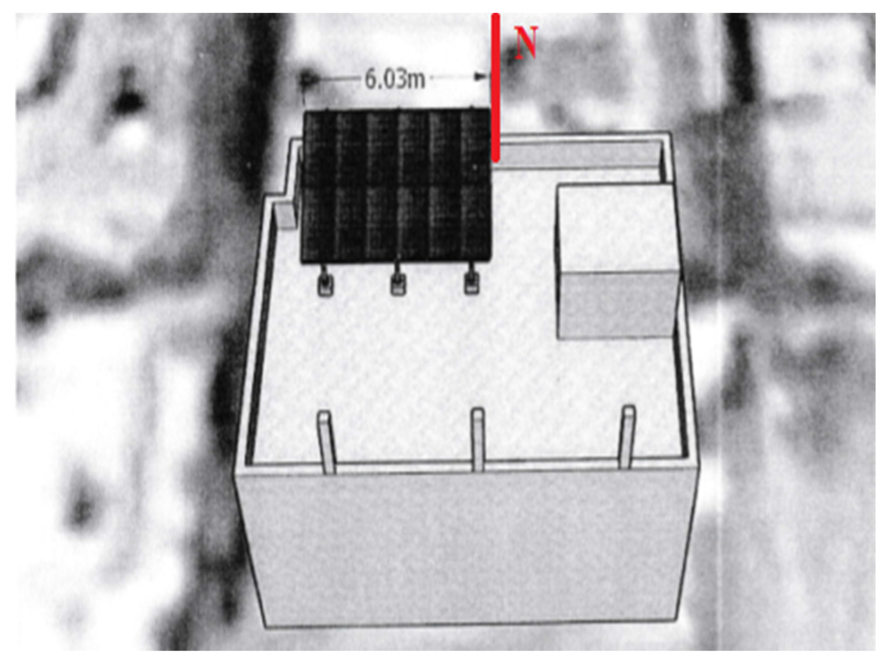
In the case of LV applications, a precise forecast model is needed, focusing on comprehending electrical demand behaviour and examining interrelatedness among external variables and demand. In the case of household energy demand and PV behaviour, this section will analyse and review the data that will be used to develop and evaluate the forecast models. In addition, this section will investigate the common model connections among household electrical demand in Jordan and various external variables, for instance, demand seasonality and temperature. The main outcomes will be used in the next section of this study to establish and determine the best parameters to create a precise forecast model. In this work, the main concern is individual LV demand, therefore household demand with PV has been considered. The measured data were collected at ten induvial houses located in Jordan, Al-Zarqa. The location of the houses is within a 2 km diameter from 32°04′27.9″ N 36°02′58.9″ E, as shown in Figure 1. The houses in this area are typical and they connected to the same size PV system. The area of the house is approximately 170 m squared, and consists of five rooms, one kitchen, two bathrooms, and balcony. Furthermore, the electrical system is single phase and the main electrical loads are three air conditioners, fridge, electrical water heater, washing machine, lights and two televisions.

PV System

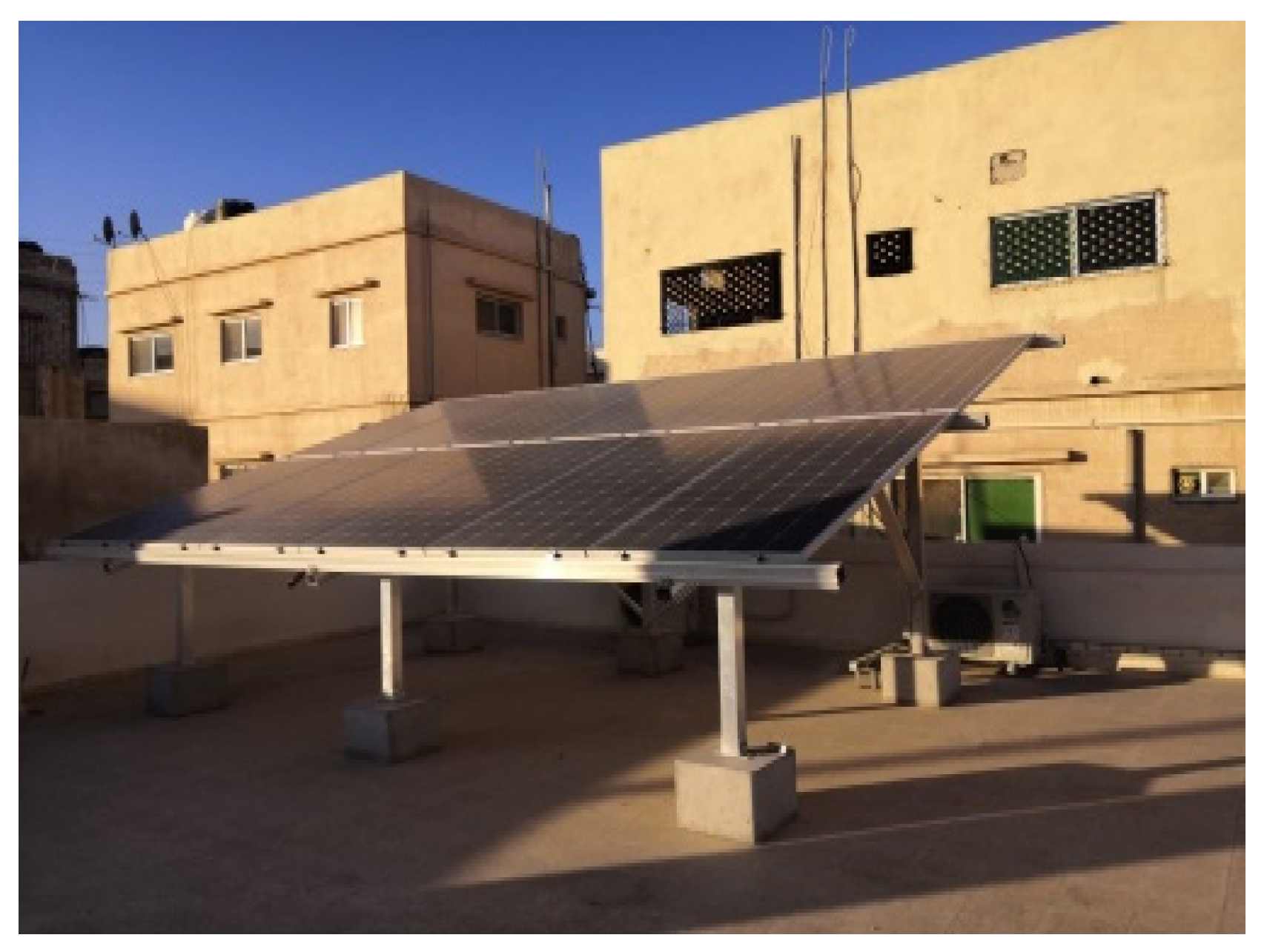
In order to reduce the electricity bill in the ten houses, each is connected to a PV system, as shown in Figure 2. The size of the PV system is 4 kW peak, which is the maximum allowed capacity from the government for household PV systems, and the main parameters of the PV system are detailed in

Table 1. Parameters of the PV system.

Content	Description	Quantity
PV panels	(Jinko) cells with 345 watt power, Mono type	12
Inverter	4 kW (ABB)	1
panel area	25 ${\mathrm{m}}^2$
Electrical Wires	AC & DC Wires	---
Other electric components	Power Panels Circuit breakers	---

. For example, the size of the PV system has been determined based on the monthly electricity demand during 2019, as shown in

Table 2. An example of monthly electricity demand over 2019 for a single house.

Month	Consumption kWh	Month	Consumption kWh
JAN	1089	JUL	1012
FEB	1080	AGU	1050
MAR	574	SEP	784
APR	544	OCT	510
MAY	866	NOV	644
JUN	870	DEC	900

.

3. Data Analysis

In most cases, the designing of the prediction model did not normally occur at a single stroke. Accordingly, it is needed to recall former steps as a first procedure, then check the model during the training levels and both models for parameters and variables. Thus, it is important to divide the data group into three sets: validation, training, and testing. Commonly, these sets can be utilized as training model parameters, locating required patterns in the case of the training set, while the validation set is utilized in the finest model. A trade-off between reaching precise model parameters and preventing overfitting is needed to guarantee a suitable data size. The smart meter data for ten households and PV systems were collected over the period 1st of January 2019 to 30th of November 2020. The gathered data, at a one hour resolution for household demand, defines real daily demand and performance at the house, along with a 15 min resolution for the PV system output. The data set has been collected from the National Electric Power Grid Co (NEPCO) over a five year period up to the end of November 2020 for a small city in Jordan (Madaba). The main reason for including this data set is to evaluate forecast models over different level of electricity consumption. The first 65% of the collected data is employed to develop and train the forecast models as a training data set, 15% of the collected data is used to validate the forecast models, and the last 20% of collected data is utilized to assess the forecast models’ performance [28,29,30,31].

3.1. PV System Data Analysis

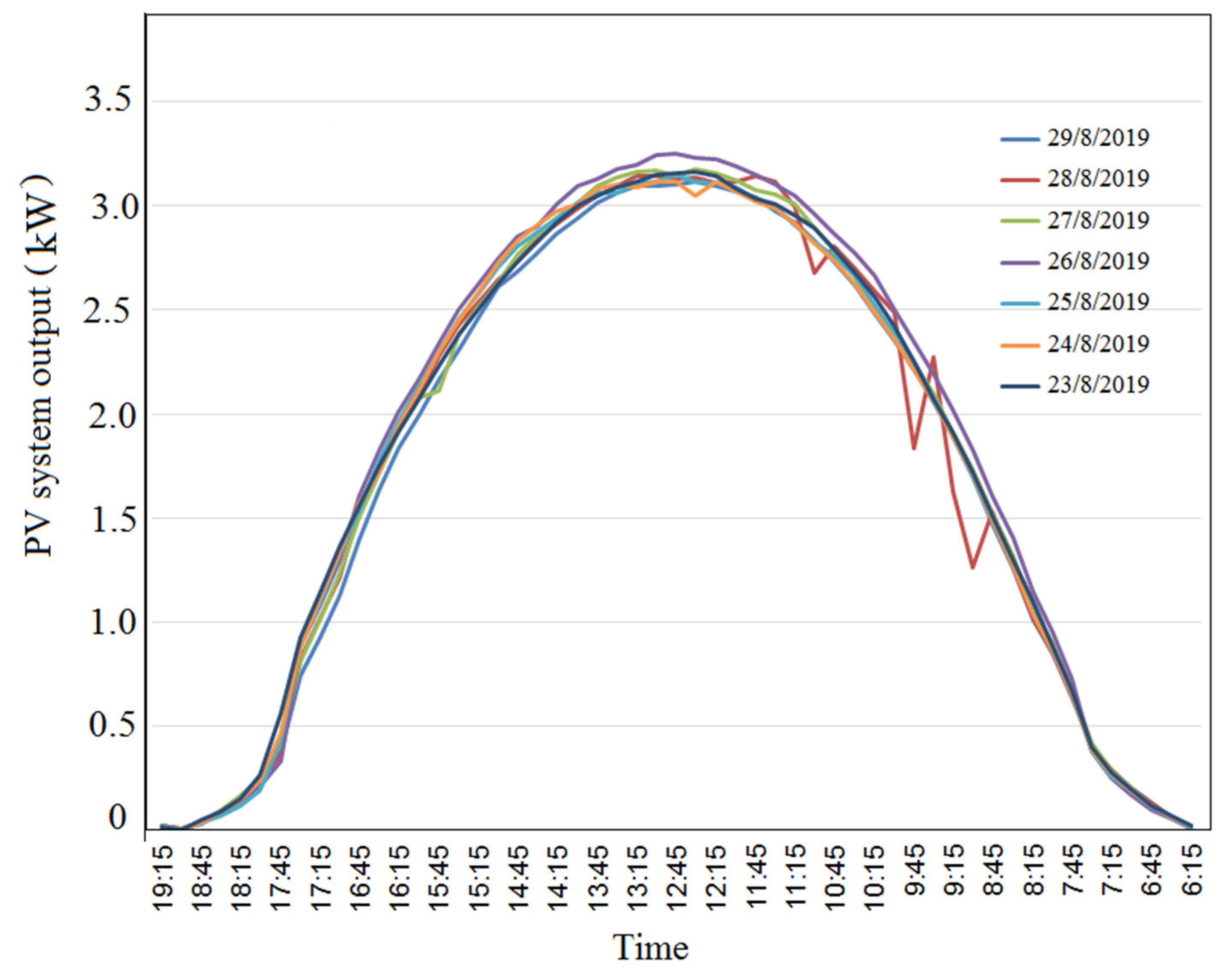
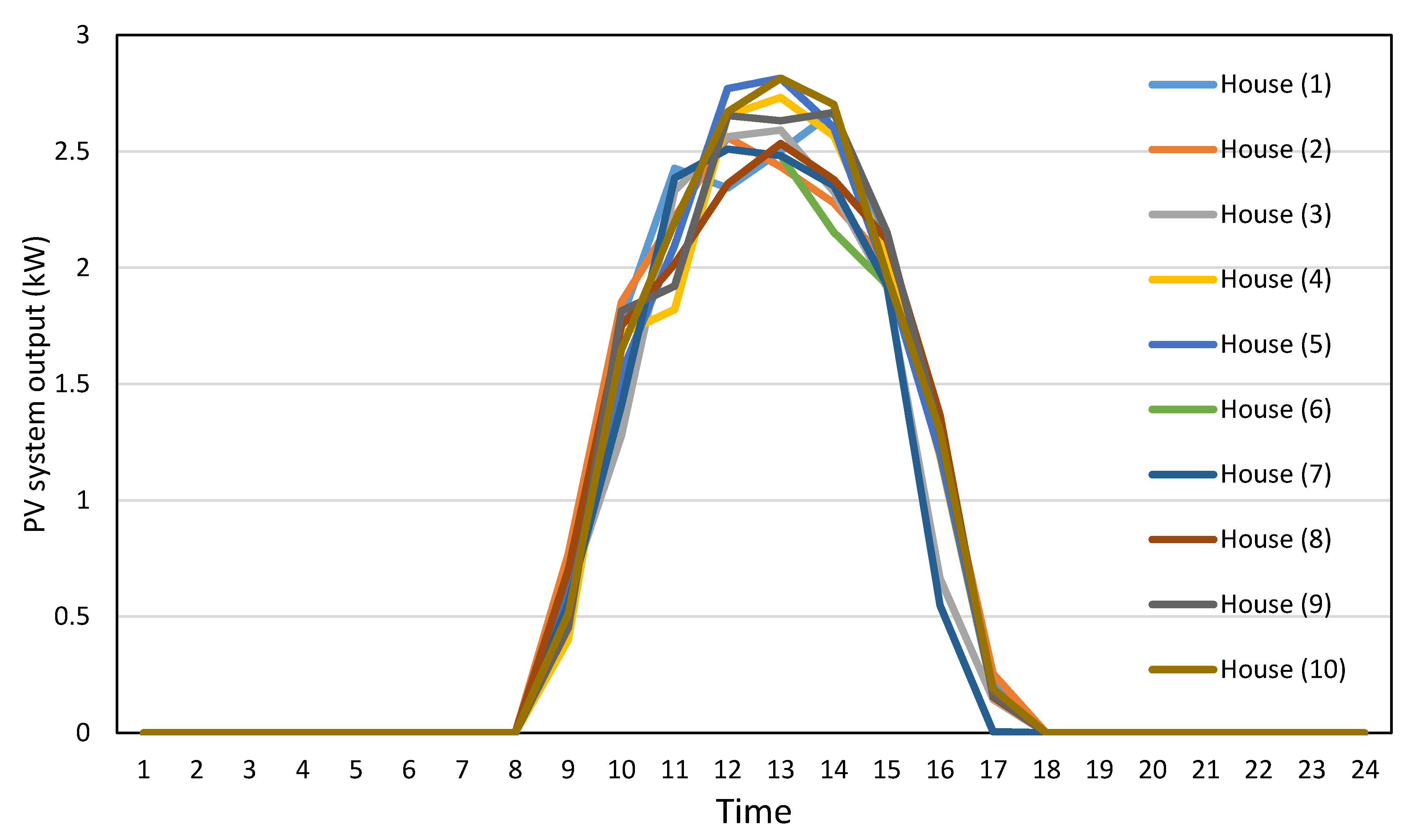
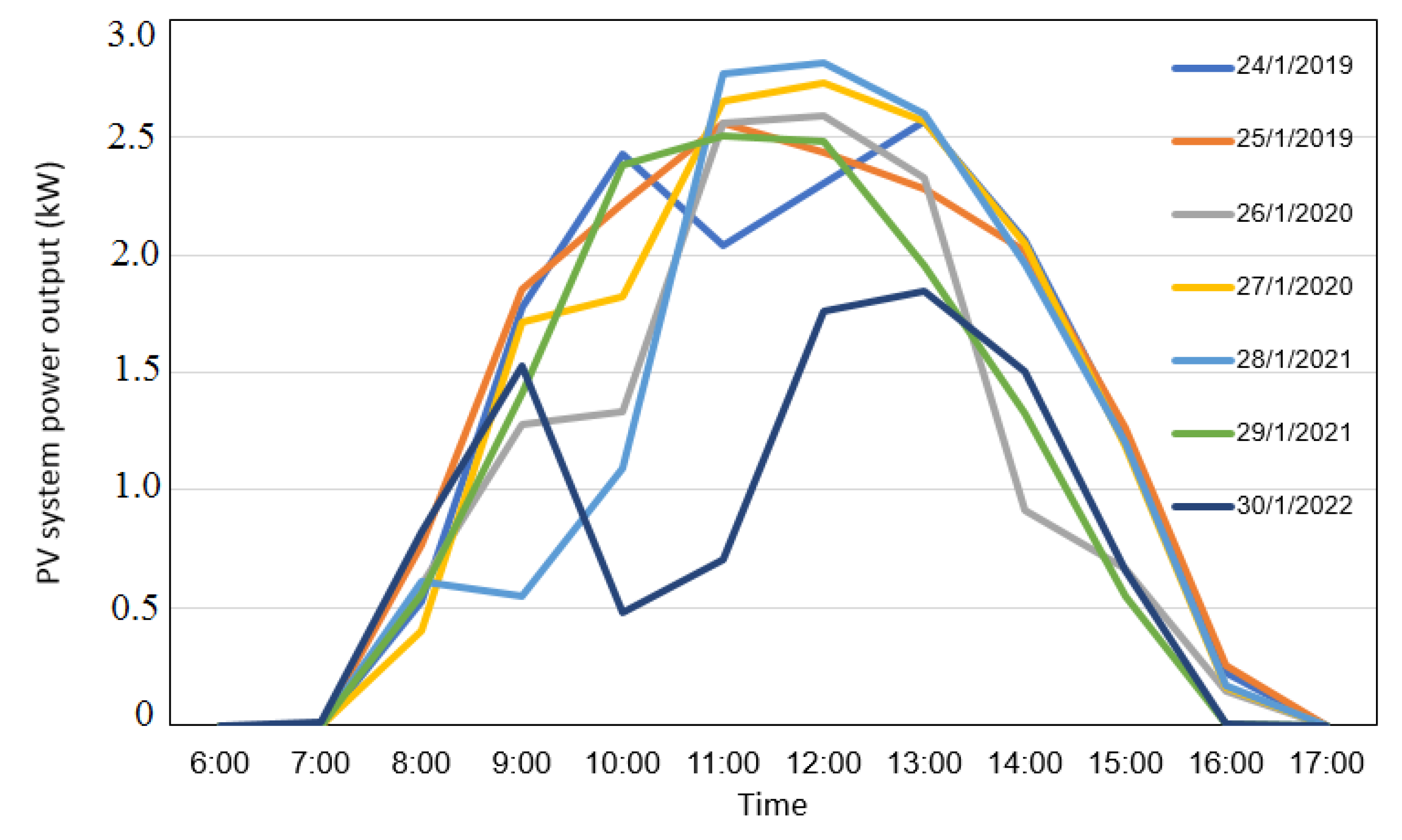
In this section, the training data set of PV output is used to understand the PV system’s behavior by employing a time series analysis to investigate whether there are any important patterns or seasonality in the data. This is significant and required in the next section, in order to concentrate on the analysis of time series by determination patterns (cycles) in PV output. The PV system data contains a strong weekly and daily periodicity during sunny days. Figure 3 highlights that all PV output curves within a week (23rd to 29th of August) have a high degree of daily regularity. Figure 4 presents the ten houses’ PV system output curves for a typical sunny day. In general, they show a convergent behavior. However, the deviation between the PV curves, as shown in Figure 4, is mainly related to the deviation in the panel’s efficiency, panel cleanliness and PV degradation. This deviation between the household PV system output curves increases uncertainty and difficulties in creating an accurate forecast model. On the other hand, Figure 5 shows a case of the PV system output profile for more than one week during the winter season in Jordan. The daily PV profiles are different from day to day where depending on the weather conditions. For instance, the maximum power output on 28th of January 2019 was 2.8 kW, but was 1.8 kW on 30th of January 2019. Besides, it is unclear from Figure 4 that there is an indication of peak output occurring at one point in the day. The peak PV output on 27th of January was 2.8 kW at 12:00 p.m., but was 1.7 kW and 2.3 kW on 24th and 30th of January at the same time, as illustrated by Figure 5. These findings support the fact that the PV output is extremely volatile in light of the absence of weekly/daily patterns or recurrences of unclear sky duration.

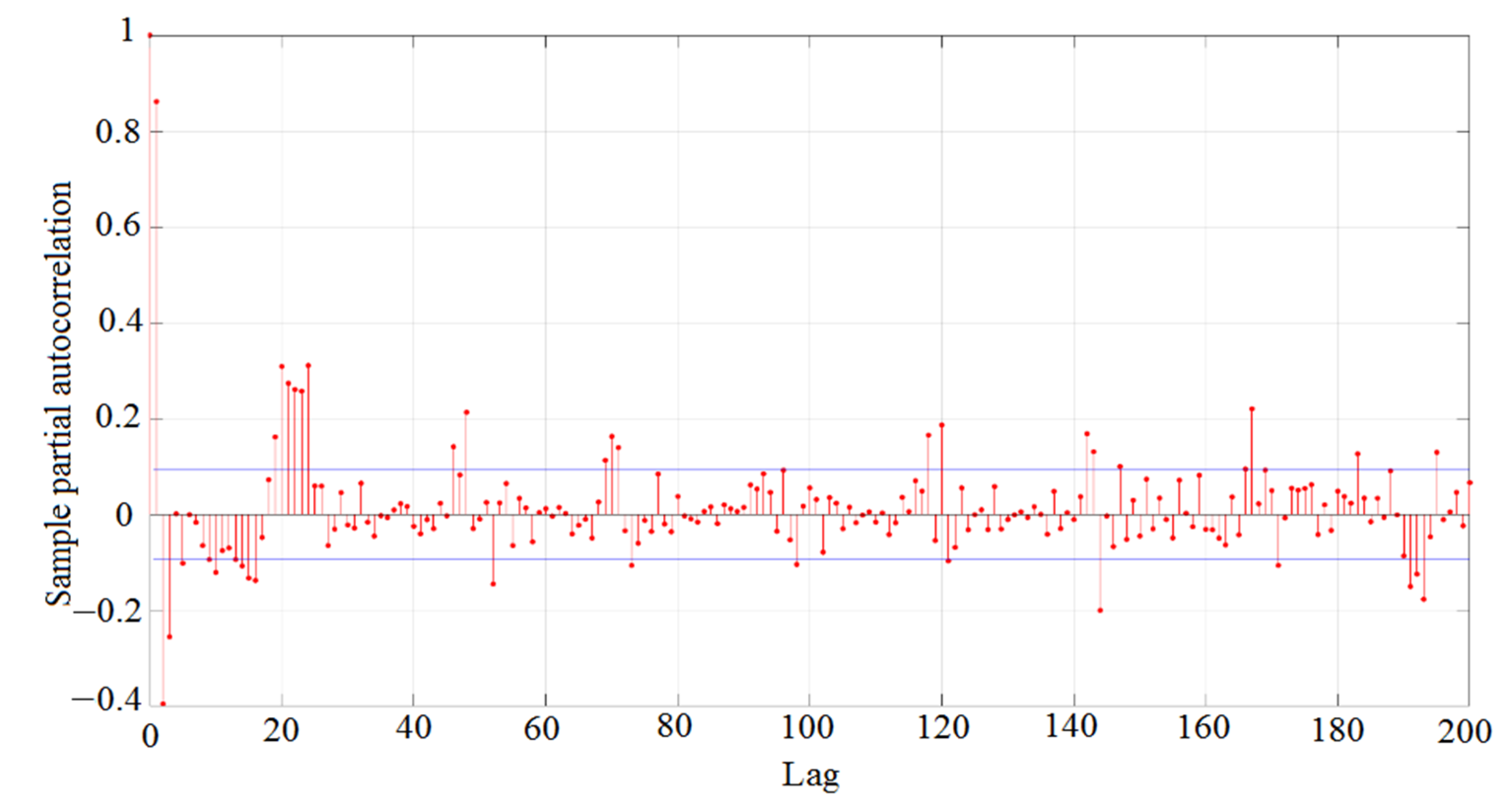
The preceding analysis demonstrates that there is no daily and weekly seasonality in unclear sky conditions compared to the daily pattern during sunny days. Thus, this section aims to identify if the behavior of patterns (daily or weekly) can be classified as special PV output. In this case, the time series points are investigated to find the links (patterns) between them, which can be collected via the Partial Autocorrelation Function (PACF) through 200 time lags, as illustrated in Figure 6. The significance of calculating the PACF is to find any links that can have iteratively taken place. As illustrated in Figure 6, the plot of PACF has demonstrated the correlations among the PV power output time series at $P_{ }\left(\mathrm{t}\right)$ for up to 200 (fifteen minutes) lags. In general, the calculation of PACF aids in finding any links via the two direct variables, irrespective of the impact of all retardation (lags) times [32,33,34]. Following lag number 3, a chop-off is manifested as demonstrated in the PACF plot with another negative impact represented among 10–20 lags. From the PACF plot (for unclear sky days), there is no obvious pattern or seasonality when observing the distribution of lags, especially when comparing with sunny days that usually exhibit considerable lags within 48 or 96. The considerable lags in Figure 6, are likely to be due to random salience and they could be related to the continuity of sunshine more than to a single time step. The time series examination indicates that the PV power output unprovided a clear daily or weekly seasonality, leading to more challenges in forecasting the PV output as a result of the non-smooth performance of power curves. This is mostly related to weather conditions; therefore, another consideration should be to comprehend the volatility of the true data.

3.2. Weather Data

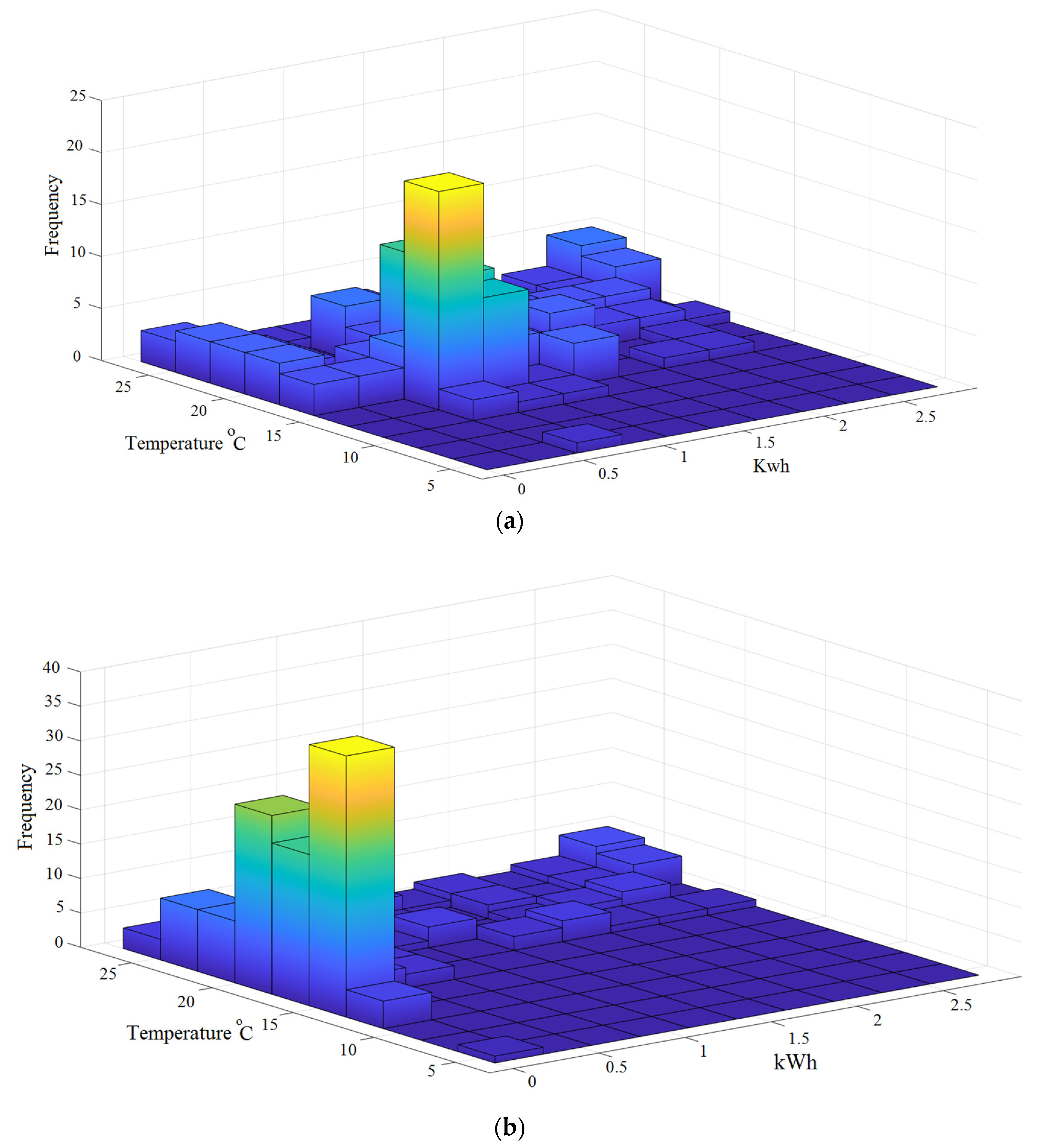
Weather variables such as temperature and wind are usually considered within load forecasting models [35,36,37] However, it is not obvious that weather conditions have a significant role in forecasting renewable energy sources or LV demand. In this paper, the hourly temperature data has been collected over the training and testing period. In order to minimize the impact of the non-smooth behavior of the power curve on the forecast model, especially during unclear sky conditions, this section focuses on the relationship between weather variables, household demand and PV power output. Figure 7 displays the 2D histogram of the weather variables, household demand and PV power output data sets over one week. Every one of the histogram bins (bars) shows the joint distribution and correlation of the data sets. Figure 7 shows strong correlation between temperature, demand and PV power output curve. In Figure 7a, the higher frequency for household demand occurred between (0.5–1) kWh and (12.5–20) temperature. In addition the higher number of observations for hourly PV power output was (0–0.25) kW when temperature was equal to (12.5–20) °C. For the PV system, the higher power output (2–2.5) kW occurred when the temperature was equal to (20–25) °C. This was expected as the rated (designed) power output of PV is generated when temperature is 25 °C.

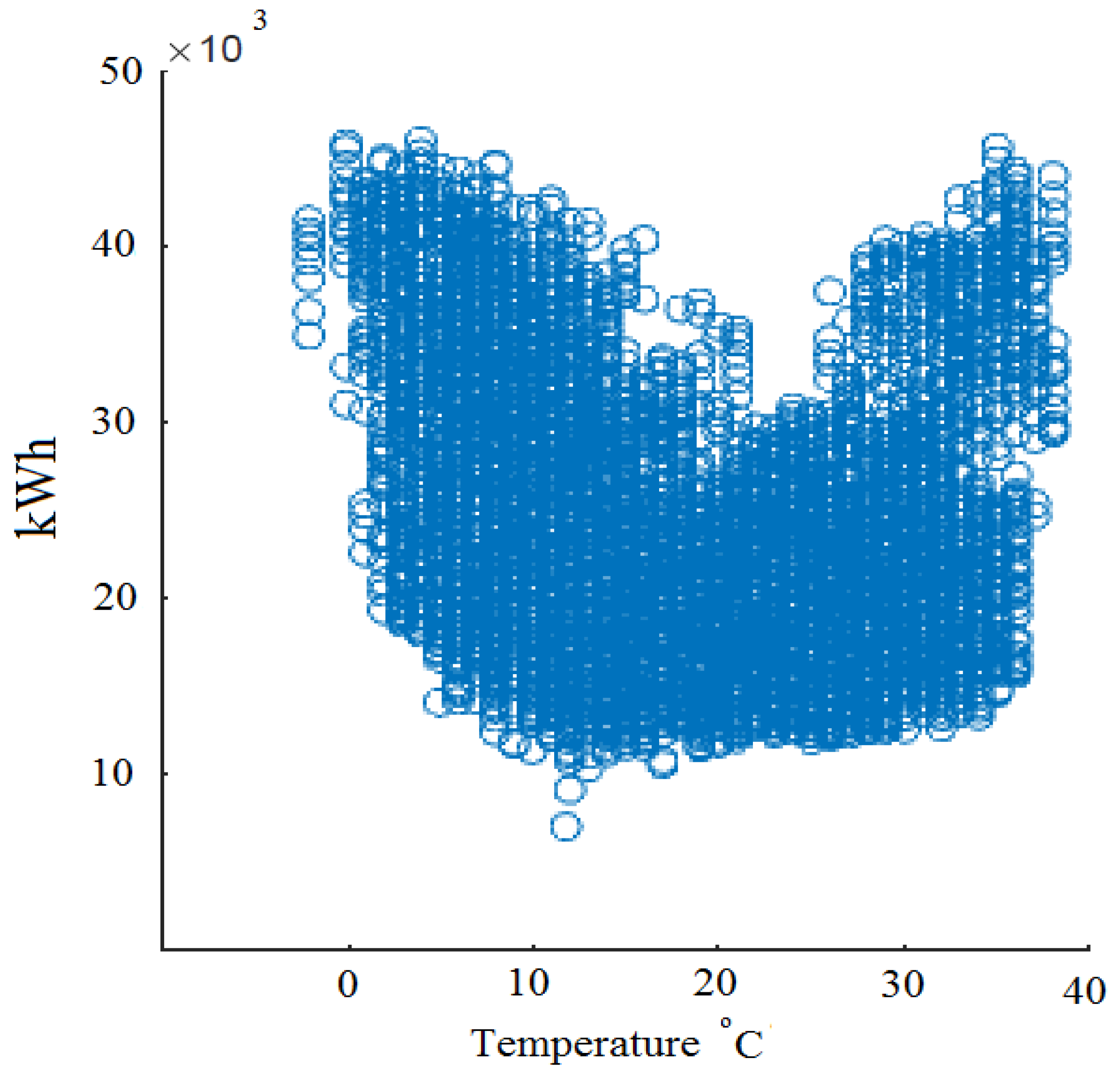
The relationship between the hourly demand and temperature, °C, is visualized through a scatter plot as seen in Figure 8, for Jordan (Madaba). In this figure, it can now be seen that, for temperatures less and more than 20 °C the demand increases. The increasing demand rate is slower for temperatures less than 20 °C compared to temperatures above 20 °C. Figure 7 shows evidence for annual demand seasonalities and correlation between demand and temperature time series. The demand has high values at high and low temperatures during winter and summer seasons. Demand increases in winter and summer due to the use of electrical heating and air-conditioning. It is clear then that the temperature and the demand series are correlated.

Table 3. R-squared values for the relationship between hourly temperature and wind speed with the PV system output.

Correlated Variables	$R^2$
$\mathrm{PV} \mathrm{output}$ vs. temperature	94.5%
$\mathrm{PV} \mathrm{output}$ vs. wind speed	39.3%

presents the R-squared value for the linear relationship between the hourly temperature and wind speed and the PV system output. The ${\mathrm{R}}^2$ statistical analysis introduces high correlation between temperature and the PV system output and direct proportionality between these variables, with ${\mathrm{R}}^2$ equal to 0.94. In the case of wind speed, the ${\mathrm{R}}^2$ value becomes 0.39 which shows that wind speed has less ability to explain PV output variability compared to temperature. However, the wind speed, as a natural cooling system for PV panels, helps to increase PV output, which explain the positive linear relationship between them.

3.3. Load Data Analysis

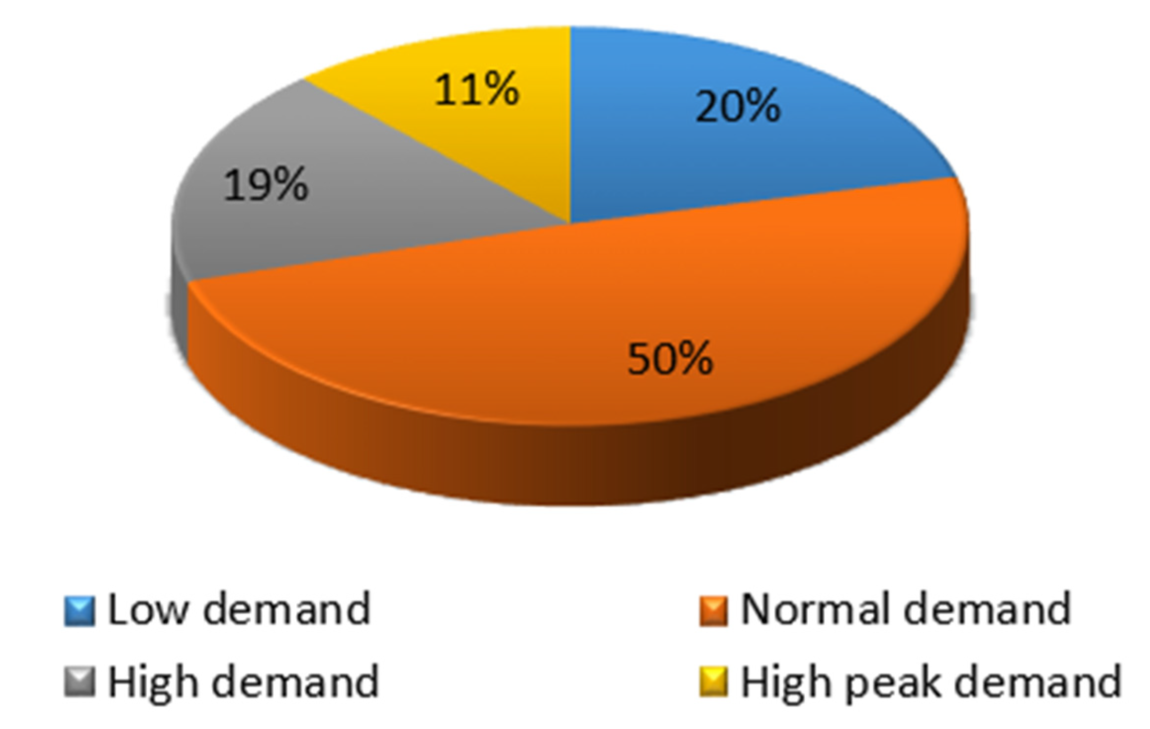
In order to provide an overview of the demand data, investigation of the ten households data is demonstrated in

Table 4. Overall statistical data analysis forhousehold demand.

Household Demand Resolutions	μ (kWh)	$\mathbf{\Sigma }$ (kWh)	CV	Maximum Demand (kWh)	Minimum Demand (kWh)
Hourly	1.6	1.40	87.2%	6.9	0.0
Daily	37.1	15.1	38.3%	63.7	15.2

, showing demand statistics comprising average demand, $\mathsf{\mu }$, and standard deviation, $\mathsf{\sigma }$. Furthermore, to exhibit the extent of unevenness at hourly and daily resolutions among both mean and standard deviation where the coefficient variation (CV) is further recognized, a relative standard deviation is presented in Table 4. The summary for domestic demand is demonstrated in Table 4, where the standard deviation ($\mathsf{\sigma }$) is for the domestic schedule with 1.4 kWh (hourly demand) and 15.1 kWh (daily demand). Accordingly, there is a substantial indication of greatly fluctuating and erratic domestic demand for the mean value of approximately 87.2% (hourly demand) and 38.3% (daily demand). Moreover, Figure 8 represents a substitute visualisation of the allocation of domestic demand data. In Figure 9 also, the average hourly demand can be broadly classified into four groups: (1) from 0 to 0.5 kWh as low demand, (2) from 0.5 to 2 kWh as normal demand, (3) from 2 to 3.5 kWh as high demand, and (4) over 3.5 kWh as high peak demand. A representation of demand values appearing in tie can be traced as follows: 20% as low and 19% as high, while 11% occur as high peak, as observed in Figure 9. In contrast, times with a 50% value represent the average demand consumed by households.

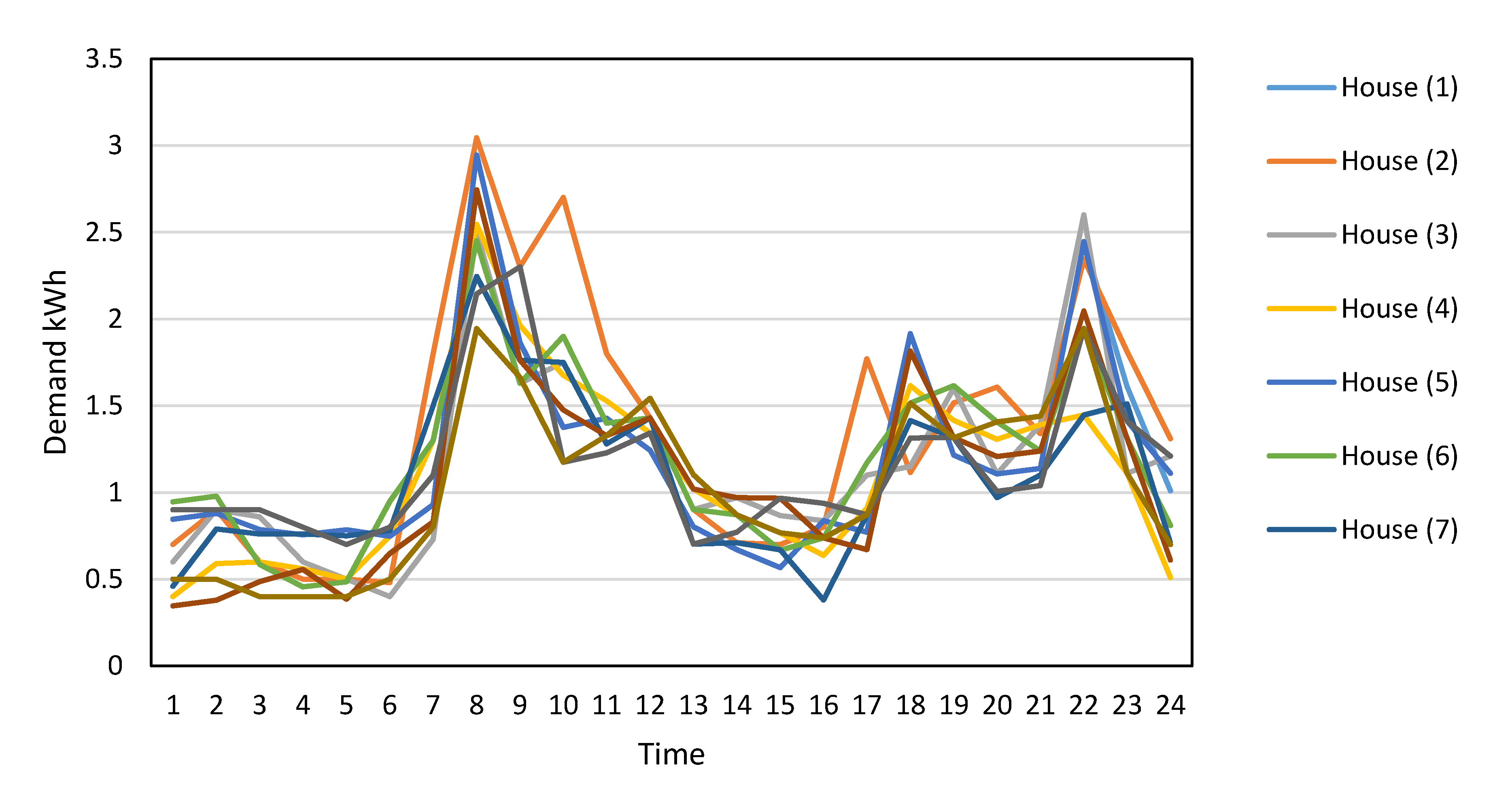
The ten houses’ demand curves for the same day (working day) are presented in Figure 10. In general, the household demand curves for the ten houses show similar behavior with two main peaks in the morning and evening, popular behaviour for household demands [17,23]. However, a wide deviation between the demand curves at the same time is shown in Figure 4. For example, house (5) achieved morning peak demand equal to 3 kWh compared to 1.9 kWh for house (10) at 8:00 and 2.7 kWh for house 2 at 10:00. This deviation is mainly related to the deviation in householders’ behavior in consuming electrical energy. This deviation at individual energy user level increases the uncertainty and the difficulties of creating an accurate forecast model.

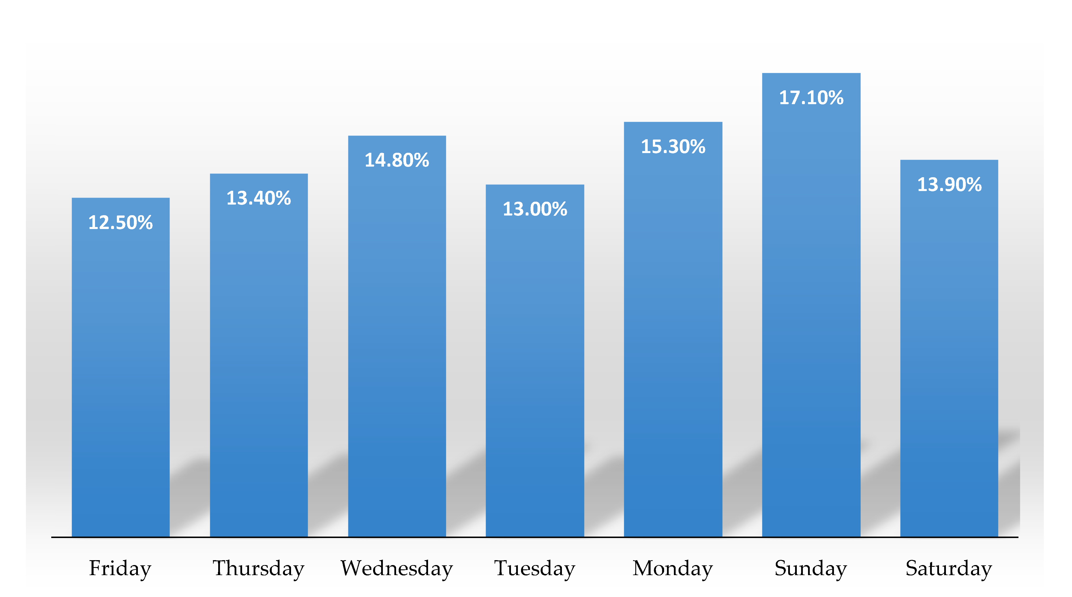
On the other hand, for the aggregated demand profiles, as in the data collected from Madaba city, the load profile is usually smoother and more predictable with an annual seasonality pattern [17,23]. A detailed demand analysis for this level of aggregated demand is presented and discussed in [23]. Therefore, the following analysis aims to investigate the cycle or pattern on a daily and hourly basis which was not discussed in [23]. Figure 11 presents the total demand patterns related to the days of the week at Madaba city. It is clear that the total daily demand percentage is similar over all weekdays but not on Sunday, with a highest demand percentage of 17.1% from total weekly demand. In Jordan and the Middle East, Sunday is the first working day in the week and the weekend (non-working days) is on Friday and Saturday. In general, there is no obvious pattern of daily distribution over the week while total demand values are similar.

3.3.1. Composition

Table 5. R-squared values for the relationship between current and lagged demand at Madaba city.

Correlated Variables	${\mathbf{R}}^2$
$(\mathrm{t})$ vs. $\mathrm{L} (\mathrm{t}-1)$	89.5%
$\mathrm{L} (\mathrm{t})$ vs. $\mathrm{L} (\mathrm{t}-2)$	76.7%
$\mathrm{L} (\mathrm{t})$ vs. $\mathrm{L} (\mathrm{t}-3)$	59.3%
$\mathrm{L} (\mathrm{t})$ vs. $\mathrm{L} (\mathrm{t}-4)$	22.9%
$\mathrm{L} (\mathrm{t})$ vs. $\mathrm{L} (\mathrm{t}-24)$	45.6%

presents the R-squared value for the relationship between the current demand $\mathrm{L}$(t) and the lagged demand L (t − i). The highest ${\mathrm{R}}^2$ value was 0.89, which shows a high correlation between the current and previous hour’s demand. This correlation can be used as main input for the forecast model, however, it will require updating of the measurements in every time step. The ${\mathrm{R}}^2$ increased gradually from 0.22 to 0.89 in line with the decrease in the (i) value. This means the linear model will be less able to explain demand variability when depending on the high (i) lag value and this correlation will not be an effective relationship in forecasting load. However, the ${\mathrm{R}}^2$ value for the previous day’s demand at the same time shows a positive, strong correlation, with value equal to 0.45.

3.3.2. Time Series Analysis

The MV network demand usually demonstrates a substantial weekly/daily seasonality, using the time series analysis [38,39]. The current section will examine in detail the energy usage of a single household through the training data period by demand profiles to ensure that it follows either pattern or significant seasonality in demand curves. The former section provided an undetailed examination of demand, which concluded with the observation that demand values can be further sorted into a distribution with unregularly proclivities. The following factors will be taken into consideration in determining the type of cycles or patterns in the case of household demand by using time series analysis:

• Analysis based on daily and weekly patterns, to examine, if applicable therein, hour/day–day/week–week demand and any formation of cycles.
• Analysis of autocorrelation and hourly energy consumption to investigate if there are any seasonal patterns, especially those not in day/week cycles.

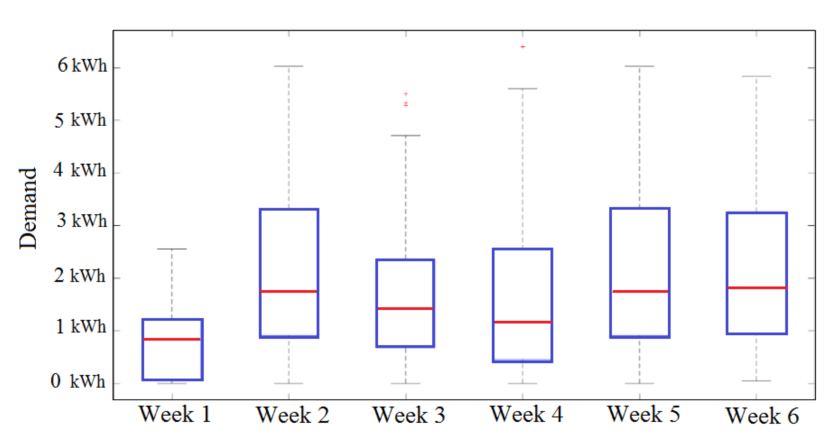
Firstly, the energy consumption profiles were introduced to probe the patterns of a weekly and daily type. A general analysis of distribution of hourly demand within week/day patterns is given in Figure 12 and Figure 13. As an example, the hourly demand over six weeks are explored in Figure 12, where the box plots symbolize demand during the dataset per every week. It can be seen from the dataset that the location of points from 0.8 kWh to 1.75 kWh is the median related to the six-week period. Besides this, the comparative values between the maximum and minimum of the median demonstrate a rise to 118.7%. Additionally, the value within one week of the Interquartile Range (IQR) also varies greatly. By way of illustration, the minimum and maximum of the first week has IQR from 0.9 to 3.2 kWh as against the second week with an IQR from 0.1 to 1.2 kWh with median 0.8 kWh and 1.75 kWh, respectively. This presents irregular behaviour in demand without apparent reference to weekly seasonality, nor week-to-week uniformity.

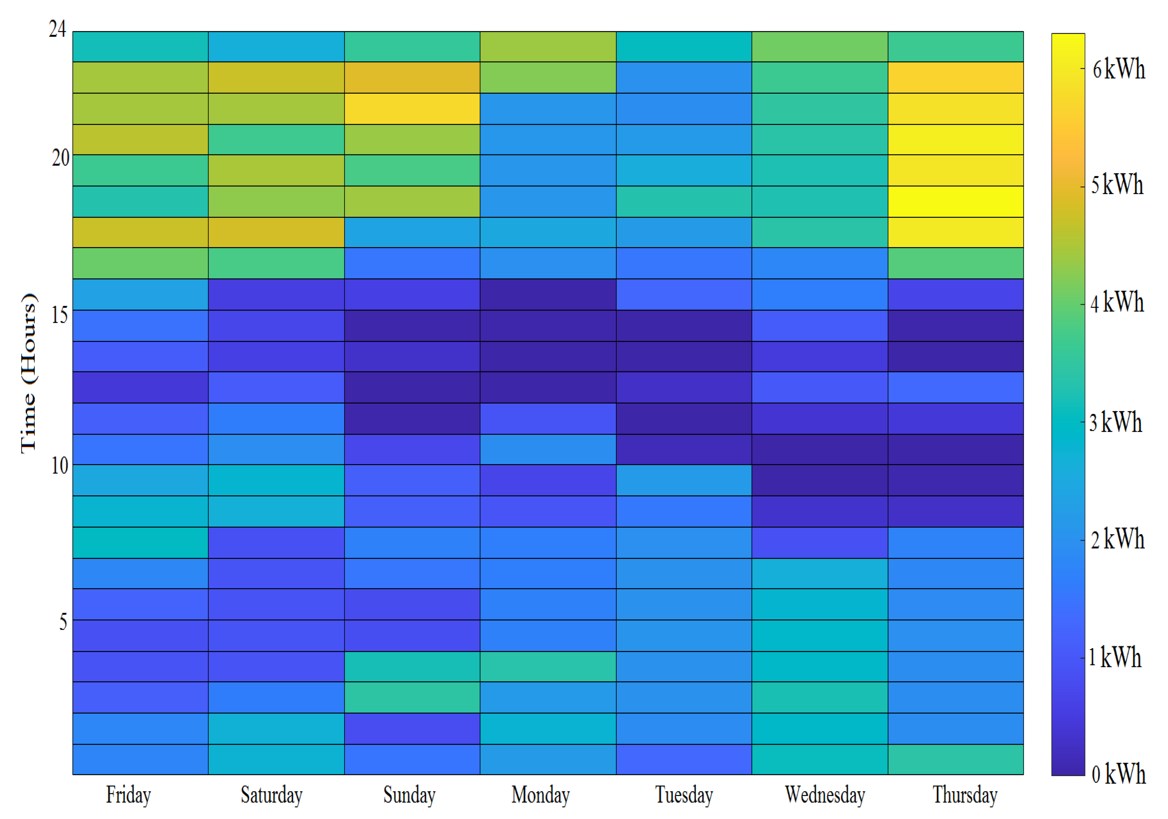
As seen in Figure 12 and Figure 13, the weekday patterns can be examined by plotting the hourly demand distribution on the basis of the sort of day. It is shown that the hourly data set consists of two patterns (categories) as addressed in Section 3.3. The first ranges from 70% below 2 kWh, while the other ranges from 12% at over 3.5 kWh. This can also be presented within several demand distributions on every type of day. Nevertheless, the observations of low demand on six days are greater than the number on Friday which ranged from 0 to 0.5 kWh. Furthermore, the demand analysis through type of day indicates that there is no specific day which has an obvious highest or lowest demand value, but every day has a broad spectrum of demand records. There is no obvious pattern of daily distribution while the highest and lowest demand values can separated into particular days. However, low demand values occur highly between 10:00 to 15:00 over the week except for Saturday and Sunday. This is due to the fact that the single household is normally highly volatile compared to aggregated demand profiles for LV feeders or MV demand [29,40], where any small activity in the household can change the load profile behaviour.

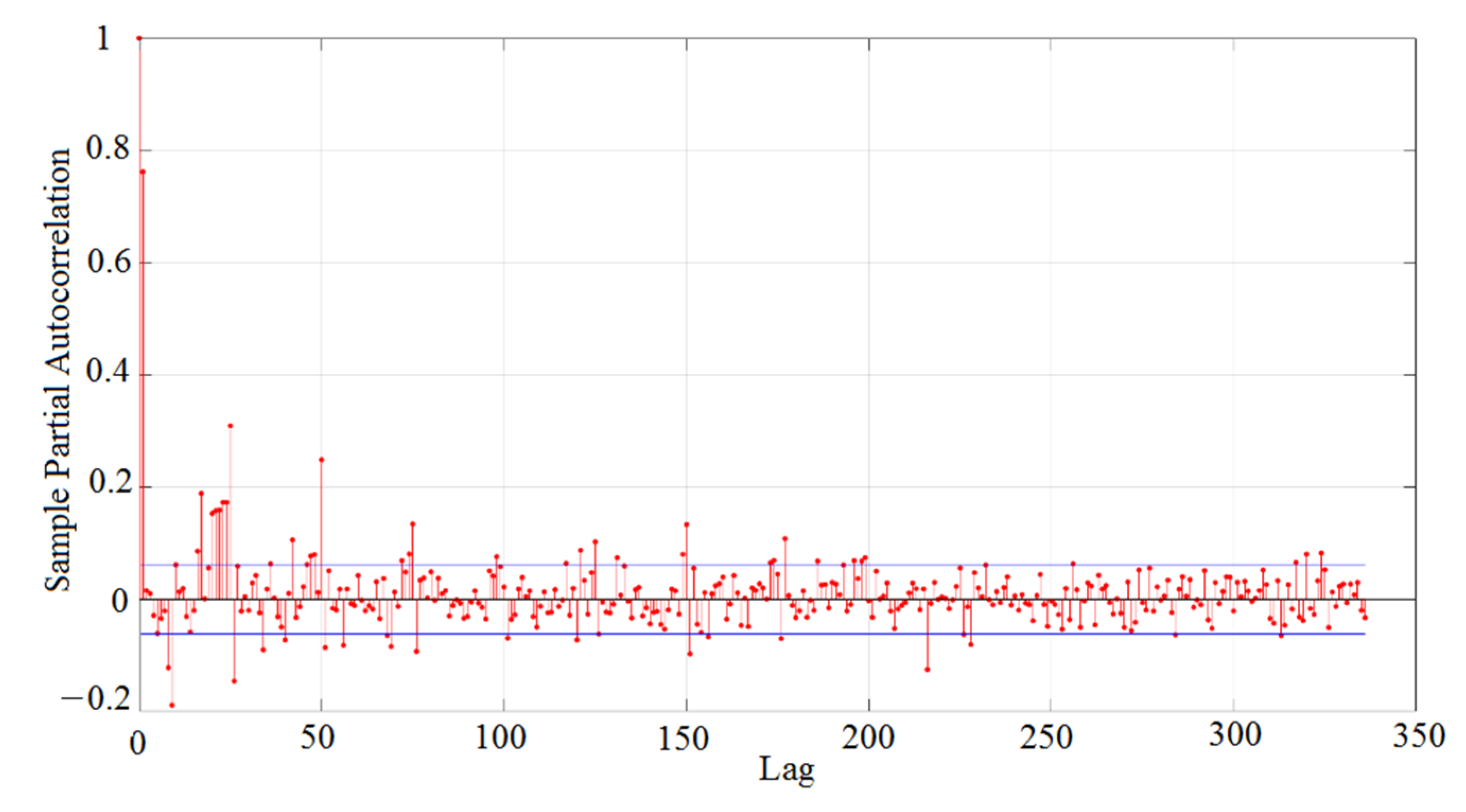
Secondly, the behavior of unsteady and erratic household demand against aggregate LV or MV demands provides challenges in seeking for seasonality models. Therefore, this section is intended to examine cross-relationships over the training data set period. The PACF was determined through two-week lags (336-time lags) in order to locate any links or patterns via the time series points, which can be seen from Figure 14. From the PACF plot, there are no obvious models or seasonalities for allocation of the considerable delays (lags) against other aggregated LV demands, that in most cases demonstrate remarkable lags (24 and multiply). Despite this, early correlation lags were randomly distributed, without an obvious automatic association performance through time series on demand. These linked lags may appear as a result of house tasks which require a further one-step time to accomplish.

In general, this section has introduced and investigated household demand and PV power output characteristics which are important to comprehend the data profiles’ performance for the purpose of improving a load forecast model in view of the current paper. The essential contribution of the existing section is to address the absence of a theoretical foundation in most of the literature for energy demand performance regarding two issues: (1) single household and (2) PV system techniques. This is crucial in promoting the load forecasting algorithms in Section 3. This section introduced an examination of time series in the case of household demand and PV system in order to check if there are any trends/models and correlation with external parameters. In addition, both the PV system and weather conditions demonstrated a high correlation, instead of any obvious indicator of trends/patterns through the data profiles. Furthermore, an explicit influence on the improvement of the forecast models is enhanced by the analysis of both cross-correlation and time series, as illustrated in Section 3. To obtain an adequate load forecast for the household demand and PV system, we must determine the ideal variables. For instance, to specify and select the greatest orders of the ARIMA variables (p, d, q), time series analysis and a PACF plot are needed.

4. Load Forecasting Models

In general, load forecasting models are utilized to anticipate fluctuating demand and might assist in achieving greater performance for low voltage implementation [1,2,3,4,5,10,11,12]. This section ought to improve different ANN forecasts and time series models. As illustrated in Section 3, given the fluctuating performance for household demand, Madaba city demand and PV system outputs compared to low voltage or medium voltage demand, the prediction challenge introduced for this specific task is more difficult and complex. In this section, forecast models are expanded to anticipate a domestic demand $\hat{\mathrm{L}}\left(\mathrm{t}\right)$ for the next hour, and PV system output power $\hat{\mathrm{P}}\left(\mathrm{t}\right)$, that is, at t + 1 until $\mathrm{t}+24$, where $\mathrm{t}$ represents the time step. In this paper, it is important to provide historical records and forecast where or not the equations whether have a (^) notation. Figure 15 illustrates a general diagram for the suggested load prediction procedures. In subsequent sections, various ARIMAX and ANN are improved, using probabilistic and new optimization approaches, respectively, as presented in Section 4.1 and Section 4.2.

4.1. Probabilistic ARIMAX Forecast Model

In general, the ARIMAX approach is defined as a statistical method using a time series that can develop historical data as a time function to estimate a specified future value. The linear and simple approach to the Auto Regressive Integrated Moving Average (ARIMA) is used as being easier to implement and does not need any historical information via time series. Moreover, the latter method can be broadly employed in predicting electrical load demand. So that the model has an external variable, the ARIMA should be modified to the ARIMAX version which consists of a nonlinear relationship and external variables. Typically, the merits of an external variable can be seen by establishing an additional parameter which assists in reducing prediction errors and increasing the use of accessible data. For the prediction of LV demand both ARIMAX and ARIMA models are common through time series [8,32]. To produce a non-seasonal ARIMAX model with (p, d, q) variables as illustrated by Equation (1) for household demand as an example, combination is needed, via a variation component with the ARIMAX model. Besides, this variation can be implemented repeatedly to create a chain constant [33,34]:

$${\hat{\mathrm{L}}}^{\left(\mathrm{d}\right)}\left(\mathrm{t}\right) = \sum _{\mathrm{j}=0}^{\mathrm{h}}{\mathsf{\phi }}_{\mathrm{j}}{\mathrm{X}}_{\mathrm{j}}\left(\mathrm{t}\right)+\sum _{\mathrm{i}=1}^{\mathrm{p}}{\mathsf{\varphi }}_{\mathrm{i}}{\hat{\mathrm{L}}}^{\left(\mathrm{d}\right)}\left(\mathrm{t}-\mathrm{i}\right)+\sum _{\mathrm{i}=1}^{\mathrm{q}}{\mathsf{\theta }}_{\mathrm{i}}\mathrm{Z}\left(\mathrm{t}-\mathrm{i}\right) + \mathrm{C},$$

(1)

$${\hat{\mathrm{L}}}^{\left(\mathrm{d}\right)}\left(\mathrm{t}\right) ={\mathrm{L}}^{\left(\mathrm{d}-1\right)}\left(\mathrm{t}\right) -{\mathrm{L}}^{\left(\mathrm{d}-1\right)}\left(\mathrm{t}-1\right),$$

(2)

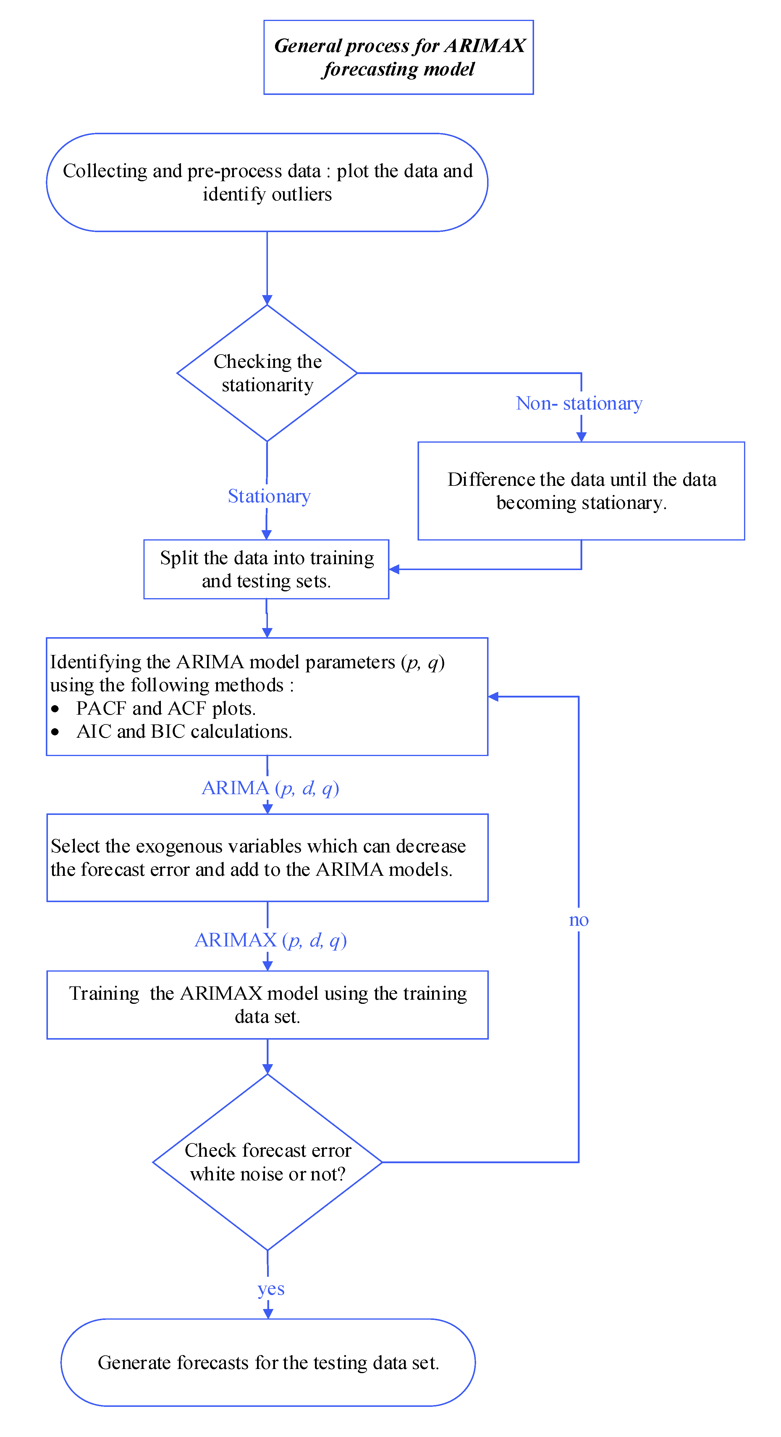
Here for ${\hat{\mathrm{L}}}^{\left(\mathrm{d}\right)} \left(\mathrm{t}\right),$ where d is differenced demand estimate by time t for ${\mathrm{L}}^{\left(0\right)}=\mathrm{L}$, this can be specified through Equation (2) where ${\mathrm{L}}^{\left(\mathrm{d}-1\right)}\left(\mathrm{t}\right)$ is the previous differenced demand by time t; ${\sum }_{\mathrm{i}}^{\mathrm{p}}{\mathsf{\varphi }}_{\mathrm{I}}{\hat{\mathrm{L}}}^{\left(\mathrm{d}\right)} \left(\mathrm{t}-\mathrm{I}\right)$ is related to ${\mathrm{pth}}^{}$ order autoregressive polynomial lag ($\mathrm{AR}\left(\mathrm{p}\right)$ model); ${\sum }_{\mathrm{i}}^{\mathrm{q}}{\mathsf{\theta }}_{\mathrm{i}}\mathrm{Z} \left(\mathrm{t}-\mathrm{i}\right)$ is related to${ \mathrm{qth}}^{}$ order moving average polynomial lag ($\mathrm{MA} \left(\mathrm{q}\right))$; ${\sum }_{\mathrm{j}=0}^{\mathrm{h}}{\mathsf{\phi }}_{\mathrm{j}}{\mathrm{X}}_{\mathrm{j}}\left(\mathrm{t}\right)$ is the ${\mathrm{hth}}^{}$ exogenous variables term; ${\mathsf{\phi }}_{\mathrm{j}}, {\mathsf{\varphi }}_{\mathrm{I}}$ and ${\mathsf{\theta }}_{\mathrm{I}}$ stand for the parameter of external variables, and both $\mathrm{MA} \left(\mathrm{q}\right)$ and $\mathrm{AR}\left(\mathrm{p}\right)$ relations; also here Z (n) is defined as the previous error of prediction which can be distributed normally, and C represents a constant value. To investigate the link between both current and any external variables, it is significant to estimate an external variable in the ARIMAX model [29,32,33,34]. As previously discussed, the parameters which are computed as a task are only utilized in case they decrease prediction error [7,8,9]. In Section 3.2, the analysis of data showed a high correlation between the PV output and household demands and temperature. In addition, a positive strong correlation between PV output and wind speed is presented. Therefore, weather conditions are the external variables: ${\mathrm{X}}_1$(t) is the hourly temperature and ${\mathrm{X}}_2$(t) is the hourly wind speed. In general, the seven actions must be completed frequently in order to improve the ARIMAX model. Figure 16 illustrates and outlines the common approach to improving ARIMAX models.

Implementation of ARIMAX forecast models:

Note that the ARIMA (p, d, q) model can be extended to ARIMAX, consisting of external variables. The BIC matrix computation has also been used to select the best ARIMAX model order. The ${\mathrm{X}}_1$(t) and ${\mathrm{X}}_2$(t) here represent the external variables for the suggested ARIMAX model. The differencing term (d) in the ARIMAX model helps to stabilize the mean of the time series by eliminating trend and seasonality. In this model, it was only required to take the first difference in order to obtain stationary data, so (d = 1) in all models. The BIC matrix computed and implemented in accordance with values p between 1 and 48, q between 0 and 48, and d between 0 and 3, which can assist parameters selection in the ARIMAX model. Through the minimum BIC value the most preferable parameters in the case of the ARIMAX model can be acquired. The BIC matrix results shows that the most preferable parameters appear in the case of the ARIMAX model (p, d, q) in accordance with the accessible data for household and Madaba city demand, through lowest BIC conveyed by (p, d, q) = (2,1,2) and (1,1,2) for PV power. The ARIMA model can be derived by removing the external variables term from the ARIMAX model.

Probabilistic ARIMAX Model

The previous method was presented as a point forecast with a single estimate output for each time step [41,42,43,44,45]. However, a point forecast is mainly limited to the description of the data model and the degree of uncertainty in the data. Therefore, a forecast model which can give a detailed picture of future demand under different degrees of uncertainty is a significant model. A probabilistic estimation approach is an estimation model which gives future demand scenarios based on the distribution of data [41,45]. In this paper, an ensemble or multivariate forecast model using Monte Carlo is developed to future scenarios of household and Madaba city demand $\hat{\mathrm{L}}\left(\mathrm{t}+\mathrm{i}\right)$ and PV system output power $\hat{\mathrm{P}}\left(\mathrm{t}+\mathrm{i}\right)$. The main advantage of developing the ensemble forecast is that it takes into account the inter-dependencies and uncertainty in the data. To present the volatile and uncertain household demand and PV system output power, the ARIMAX forecast model in Section 4.1 has been modified to generate potential future scenarios by using a Monte Carlo sampling method. Here, we sample household demand $\hat{\mathrm{L}}\left(\mathrm{t}+\mathrm{i}\right)$, and PV system output power $\hat{\mathrm{P}}\left(\mathrm{t}+\mathrm{i}\right)$ from the joint probability distribution with temperature and time, as presented in Figure 6 and Figure 9 using a 2D histogram. Then, the ARIMAX model as presented in Section 4.1 is used to obtain the forecast scenarios. The basic steps for the proposed probabilistic method using the Monte Carlo and ARIMAX model are summarised as follows [29]:

• Identify the forecast model variables and pre-sample data, where usually the training data set is used as the pre-sample data.
• Specify the empirical joint distribution of household demand, PV system output power, temperature, day and time. The 2D histogram is used to select the joint distribution, as displayed in Figure 6 and Figure 9.
• A Monte Carlo sampling method is used to generate stochastic samples from the empirical joint distribution.
• Use the ARIMAX models from Section 4.1 to generate stochastic samples and obtain the model responses.

4.2. ANN Forecast Model Optimized by Using Golden Ratio Optimization (GROM)

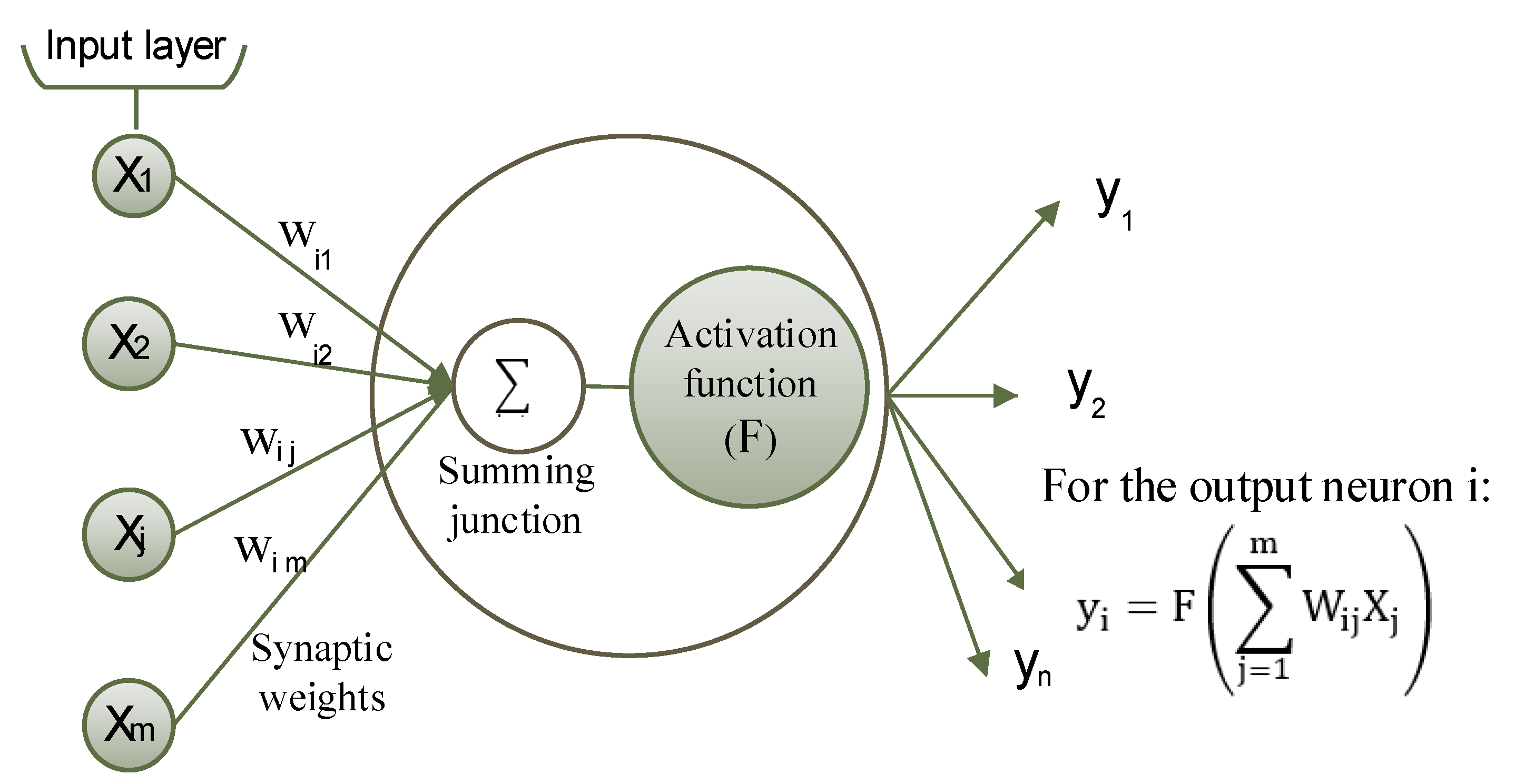
In general, the prediction of energy demand, which is a difficult and complex problem, includes many non-linear relationships such as temperature and wind speed for renewable energy applications. A range of artificial intelligence techniques are used during energy forecasting because of their flexibility and can manage complex non-linear relationships to create accurate prediction models. In general, the ANN is one of the most fashionable approaches to artificial intelligence, and it is a mathematical model that has a variety of applications that include prediction and control systems [12,40]. The idea of designing artificial neural networks is a simulation that emerged from the biological NNs of the central nervous system with a research goal of discovering how learning operates [40,41]. The mathematical models represented by neural networks consist of artificial neurons associated with synaptic weight ${\mathrm{W}}_{\mathrm{ij}},$ ${\mathrm{X}}_{\mathrm{j}}$ refers to the individual neuron among them, and${ \mathrm{X}}_{\mathrm{I}}$ is related to each neuron in the second layer [12,41]. Figure 17 illustrates the standard organization of individual artificial neurons in which the process is carried out via activation function in the summation point and gathering input-signs; in this case, the former layer’s outputs multiply through synapses [41]. Typically, in the hidden units there is a role for the activation function that can be employed in order to create an output to act as input in the following layer [6,41]. Two activation functions can be broadly classified into a hyperbolic tangent (tanh) and a sigmoid [41,42]. The objective of the scalar to scalar activation function is to model non-linearity in intricate performance and restrict the output of the neuron [41].

Implementation of traditional ANN forecast models:

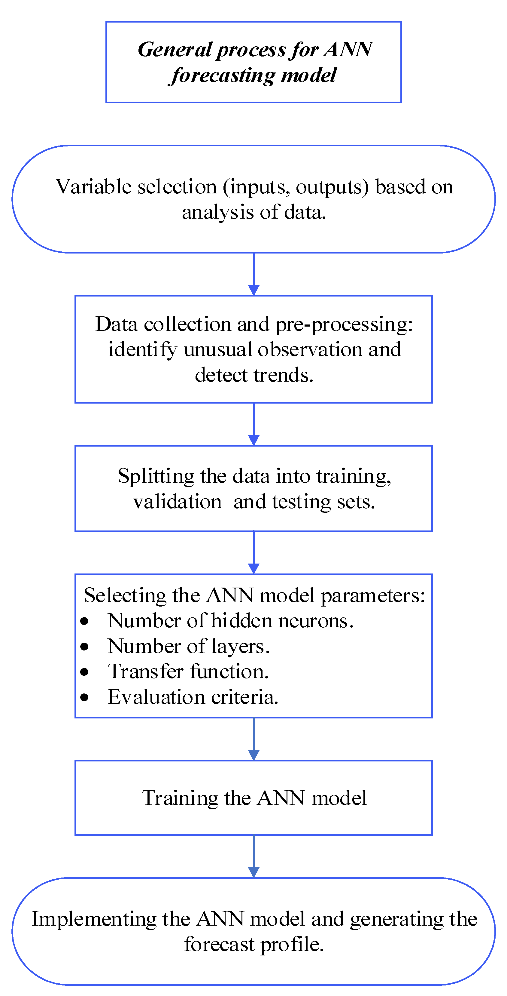
The traditional ANN feedforward model aims to forecast the future household and Madaba city demand $\hat{\mathrm{L}}\left(\mathrm{t}+\mathrm{i}\right)$ and PV system output power $\hat{\mathrm{P}}\left(\mathrm{t}+\mathrm{i}\right)$; here $\mathrm{n}$ represents the current time step and $\mathrm{i}= 1,2,\dots ,24$. Figure 18 illustrates and sums up the ANN model’s steps and introduce the standard method for ANN [6,40,41,42]. The steps of the ANN model in Figure 16 were pursued with the purpose of choosing appropriate parameter models, as listed below.

1-

Variable selection:

• Output variables: the principal goal of this paper, future demand $\hat{\mathrm{L}}\left(\mathrm{t}+\mathrm{i}\right)$, and PV system output power $\hat{\mathrm{P}}\left(\mathrm{t}+\mathrm{i}\right)$.
• Input variables: initially, the external variables (temperature and wind speed) have been carefully chosen as key input variables, by reason of the robust link amongst them and the selected output variables. Furthermore, the experimental and error method was employed to choose extra input variables grounded in the relative historical profiles and current for household demand and PV system output power. In step 4, the results and analysis of the trial and error are provided for the purpose of checking parameters.

2-

Data collection and pre-processing: the measured data is presented in Section 3. This step includes checking all data to avoid data waste. In addition, the step implies assaying the data to noise abatement, discerning trends, and finding any important link.

3-

Dividing the data set: the collected data sets are separated into training, validation and testing data sets, as discussed in Section 3.

4-

ANN model parameters selection: the capability of figuring out and alleviating the computation of complex correlations is the reason behind using parameter functions in this case study. Besides, the trial-and-error approaches apply as a consequence of identifying both numbers in hidden layers and neurons.

• Training function: Levenberg-Marquardt backpropagation.
• Transfer function: sigmoid function.
• Evaluation criteria: full squared errors.
• The stopping criteria: once there is no additional development in the error function.
• Final forecast model evaluation: the forecast performance is assessed by utilizing the MAPE in this section. The outlinedforecast model evaluation approaches are particularized in Section 4. The MAPE and each assessment forecast method are determined in Section 5.
• Input variables: in general, to improve the expected performance, a suitable external variable should be selected based on the objectives of the model and the availability of data. In Section 3.2, the analysis of data showed high correlation between the PV output and household demands and temperature. In addition, a positive strong correlation between the PV output and wind speed is presented. Therefore, weather conditions are recommended to be used as external variables: ${\mathrm{X}}_1$(t) is the hourly temperature and ${\mathrm{X}}_2$(t) is the hourly wind speed. In Section 3.3, the previous hour demand and the previous day demand at the same time showed a strong positive correlation with the current demand at Madaba; therefore, these two variables and hour of the day are recommended to be used as external variables${ \mathrm{X}}_3$ to ${ \mathrm{X}}_5$. In order to verify the impact of the proposed external variables on the forecast model accuracy, Section 5.3 presents a statistical analysis of the ANN forecast models with different external variables. The following exogenous variables are used in the PV power forecast model: ${\mathrm{X}}_1$: Temperature, ${\mathrm{X}}_2$: Wind Speed, ${\mathrm{X}}_3:$Hour of the day, ${\mathrm{X}}_4$: Former hour data and ${\mathrm{X}}_5$: Former day data in same hour. On the other hand, the following exogenous variable are used for the household and Madaba city demand forecast model: ${\mathrm{X}}_1$: Temperature, ${\mathrm{X}}_2$: Average of the previous two hours demand, ${\mathrm{X}}_3:$Hour of the day, ${\mathrm{X}}_4$: Former hour data and ${\mathrm{X}}_5$: Former day data in same hour.
• Number of hidden layers: two hidden layers.
• Number of hidden neurons: ten neurons in each hidden layer.

ANN-GROM Forecast Model

In the traditional ANN forecast model, optimization techniques such as steepest descent and the Gauss Newton method have been used in the literature [12,13,14,15,16] to solve the learning algorithm and achieve the best performance in ANN. Furthermore, these traditional optimization techniques work in finding local optimal parameters for ANN which requires that the objective function needs to simultaneously satisfy the following criteria: smoothness, continuity and differentiability. However, these traditional optimization methods cannot be efficiently used for optimizing the ANN forecast model for electrical demand with a high level of uncertainty. Therefore, it is significant to explore alternative optimization methods; to the best of the author’s knowledge, this is the first work on optimized load forecasting using the Golden Ratio Optimization Method (GROM) technique.

In the previous section, the traditional ANN load forecasting for household demand and city demand connected to renewable energy systems is presented. However, in reality the output renewable energy systems and LV demands are naturally non-smooth due to the volatile behaviour of weather conditions. Here a new optimal technique is required to efficiently achieve the best ANN performance and minimize the forecast by dealing with the uncertainties in renewable energy systems and LV demand profiles. In this paper, the Golden Ratio Optimization Method (GROM) is used to achieve the best ANN performance and optimal parameters. The GROM as a new optimization-training algorithm improved the training process by reducing the tuning time and increasing the speed to arrive at a global solution compared to traditional methods such as the gradient descent training algorithm. The GROM is an optimization solver, based on growth searching patterns nature such as those of plants [43]. The searching pattern in GROM was discovered by Fibonacci and is called the golden ratio. The golden ratio aims to determine the growth searching angle of the model which helps to improve the searching technique and achieve an optimal solution [43]. The golden ratio is used to update the searching process and find the optimal solution in two different phases. Firstly, the mean value of all possible solutions for training the ANN network (the population) is calculated; then, in terms of fitness, the mean solution is compared to the worst solution. In case the mean solution achieves a better fitness value, it will replace the worst solution. This process aims to speed up the algorithm and reach convergence. Secondly, to determine the direction of search (searching angle), a random solution will be selected and compared to the mean solution to investigate the impact of these on the search movement. This helps to determine the optimal ANN model parameters and avoid choosing additional parameters which can mislead the forecast model. In this paper, a GROM is developed to optimize the ANN forecasting model based on the following steps:

• Firstly, a number of random learning model parameters for the ANN forecast model, as population initialization is created and the mean value of the population is calculated.
• Secondly, the fitness of each model parameter is evaluated by using the learning cost function in ANN. Then, the fitness of the mean value of the population solution will be compared to the worst solution. In case the mean population solution has a better fitness result compared to the worst solution, the worst solution will be replaced by the mean population solution. This process in GROM aims to enhance the optimization speed to achieve convergence.
• Thirdly, a random solution vector is created in the population to determine and specify the new step direction and movement. The fitness of the new random solution and selected population will be compared to the mean solution. In this step, the random parameters solution aims to create a random movement towards the next step solution and to create the ability to search the whole space of the cost function. In order to select the size of movement towards the new solution and its direction, the Fibonacci formula (golden ratio) is used in this work as in [43]. The best parameters solution is the solution with the minimum objective function value. In GROM, the parameter solutions need to be updated and moved towards the best solution for the population [43].

In general, the proposed GROM optimization technique is free from any tuning steps for the optimization model, which helps to simplify the model, and reduce the convergence rate and the computational cost. In this work, the optimization model parameters have been evaluated over a wide range of values, as in [43], and the best parameters solution was determined to obtain the results.

5. Results and Discussion

In this section, the forecast model’s results are introduced and discussed. Firstly, to evaluate the performance of the proposed forecasting models over a specific time series, it is significant to determine the forecast evaluation method. The accuracy of forecasting models can be determined by using different techniques such as the Mean Absolute Percentage Error (MAPE) and Root Mean Square Error (RMSE) [1,2,3,4,5,6,7], as shown in Equations (3) and (4).

$$\mathrm{MAPE} =\frac{100}{\mathrm{T}} \sum _{\mathrm{t}=1}^{\mathrm{T}}\left|\frac{\mathrm{L}\left(\mathrm{t}\right)-\hat{\mathrm{L}}\left(\mathrm{t}\right)}{\mathrm{L}\left(\mathrm{t}\right)}\right|,$$

(3)

$$\mathrm{RMSE} =\sqrt{\frac{{\sum }_{\mathrm{t}=1}^{\mathrm{T}}{\left(\mathrm{L}\left(\mathrm{t}\right)-\hat{\mathrm{L}}\left(\mathrm{t}\right)\right)}^2}{\mathrm{T}}}$$

(4)

where $\mathrm{L}\left(\mathrm{t}\right)$ is the actual data, for example, the household demand; $\hat{\mathrm{L}}\left(\mathrm{t}\right)$ is the predicated data; t is the current time step and T is the total number of time steps (observations). The MAPE and RMSE are the most common evaluation methods for forecast models. MAPE is a scale-independency method, which makes it easy to interpret as a percentage [41]. However, if the actual data reading is zero, MAPE cannot be used because it generates undefined values. Therefore, the RMSE is used in this paper to avoid this problem during evaluation of the forecast modes. However, the RMSE, MAPE and other evaluation methods focus on the mean value of the error and do not show the forecast model performance at every time step. For example, in some cases the actual and forecast demand profiles have a close magnitude, but there is a time shift between the two profiles which leads to extremely high error value. In future work, the evaluation method for LV demand application will be updated by using an energy score model. Throughout this section, comparison evaluation of the performance of forecast models will be determined by:

• Comparing the forecast model performance over different data profiles: household demand, Madaba city demand, PV energy output and the net curve at the household, which is the difference between household demand and PV system output.
• Evaluating the impact of exogenous variables (weather conditions) on the prediction models.
• Evaluating the importance of designing a rolling load forecast model compared to a fixed forecast model, especially for volatile data profiles such as LV household demand.

5.1. Overall Comparisons

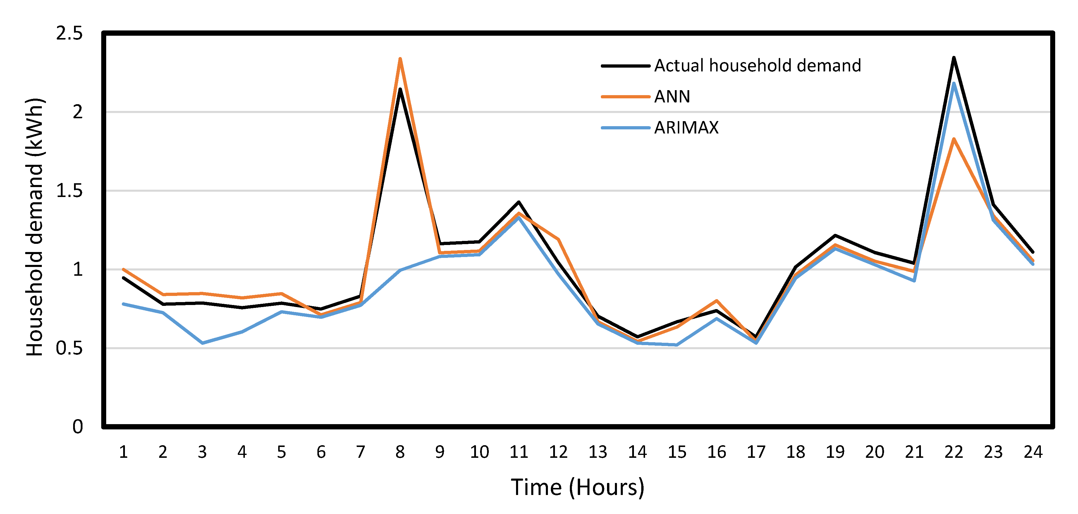
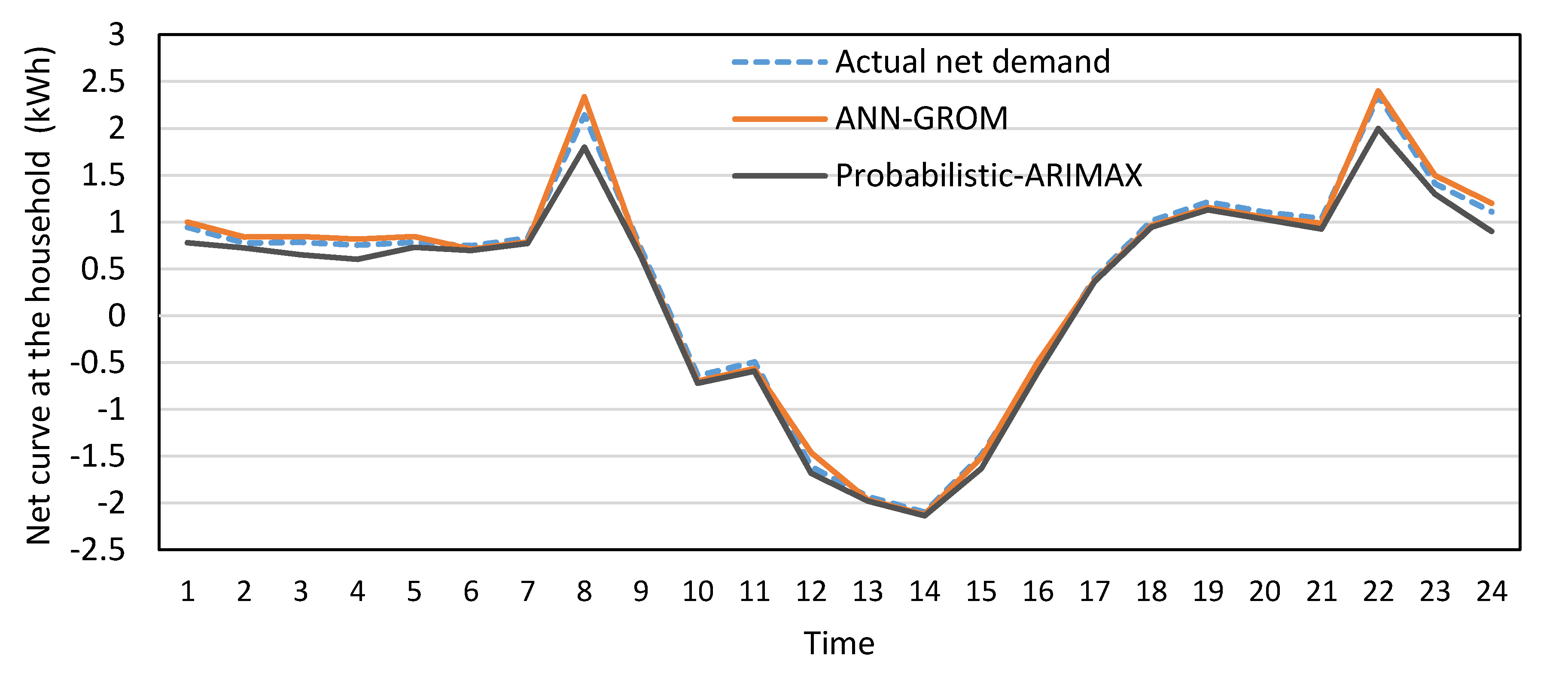
The MAPE and RMSE were calculated over the testing period for each day, as presented in

Table 6. Overall performance of the proposed forecast models.

	Traditional ANN		ANN-GROM		Probabilistic-ARIMAX		ARIMAX
	Mean Absolute Percentage Error (MAPE)	Root Mean Square Error (RMSE)	MAPE	RMSE	MAPE	RMSE	MAPE	RMSE
Household demand	5.7%	30.1 W	3.4%	20.1 W	4.7%	28.1 W	6.2%	39.8 W
PV system output	6.1%	44.9 W	4.8%	25.8 W	5.9%	31.9 W	7.1%	50.0 W
Net curve at the household	7.5%	59.8 W	5.3%	28.6 W	6.5%	40.8 W	8.4%	70.1 W
Madaba City	4.3%	860 kW	3.1%	620 kW	4.2%	845 kW	4.9%	980 kW

. The MAPE and RMSE scores of the Probabilistic-ARIMAX forecast model are based on the average demand scenario. Furthermore, the MAPE and RMSE for the household demand application are calculated based on the average of the ten houses’ results, where these results are without any significant deviation. In general, the mean value approach is one of the most common in solving stochastic problems [29]. In terms of the overall performance, the ANN-GROM forecast models provided the highest prediction accuracy for all data profiles over the testing period. Firstly, the traditional ANN and ARIMAX models’ profiles are generated for the three types of data sets over the testing period and compared to the actual data. A specific example of the actual household, net demand and prediction models’ profiles are illustrated for one day in Figure 19 and Figure 20. The ARIMAX model misses a significant peak at 8:00 o’clock and tends to underestimate the household demand, as shown in Figure 19. On the other hand, the ARIMAX and Probabilistic-ARIMAX models tend to underestimate compared to the traditional ANN and ANN-GROM models, as presented in Figure 19 and Figure 20. For all three types of data sets, the ANN-GROM and Probabilistic-ARIMAX outperformed the traditional ANN and ARIMAX models, as presented in Table 6. The MAPEs for ANN-GROM model were improved by 41.2%, 22.1%, 30.1% and 27.9% for household, PV output, net demand and Madaba city demand data profiles, respectively, compared to traditional ANN models. In addition, Table 6 shows that the Probabilistic-ARIMAX models outperformed ARIMAX by providing minimum RMSE values of 28.1 W, 31.9 W, 40.8 W and 845 kW for the household, PV, net demand and Madaba city demand data profiles, respectively. ARIMAX generated the highest RMSE value during forecasting of the net demand curve. In addition, all forecast models show a lower prediction performance during forecasting of the net demand curve compared to PV and household profiles. This is mainly due to the fact that the exogenous variables for both forecast techniques were chosen based on the correlation between weather conditions and PV and household profile without taking into account the net demand curve. Section 5.2 will present the effect of choosing the exogenous variables on both forecast models’ accuracy in more details. The ARIMA and ARIMAX was concerned with point forecasts where there is only a single estimate value is generated at each time step. The point forecast model (ARIMAX) is limited in to the demand data behavior and mainly for data with large degree of uncertainty. Instead, the probabilistic-ARIMAX give a more detailed picture of demand by generating a number of future demand scenarios, which will help to capture all possible scenarios including the worst-case scenario based on the historical data. Therefore, the mean value of probabilistic-ARIMAX showed more accurate forecast results compared to the ARIMAX, as shown in Table 6. However, the probabilistic-ARIMAX model will be limited to the number of generating scenarios and the size of available historical data. In general, increases in number generation demand scenarios in the probabilistic-ARIMAX will increase computational costs.

5.2. Forecast Error Analysis

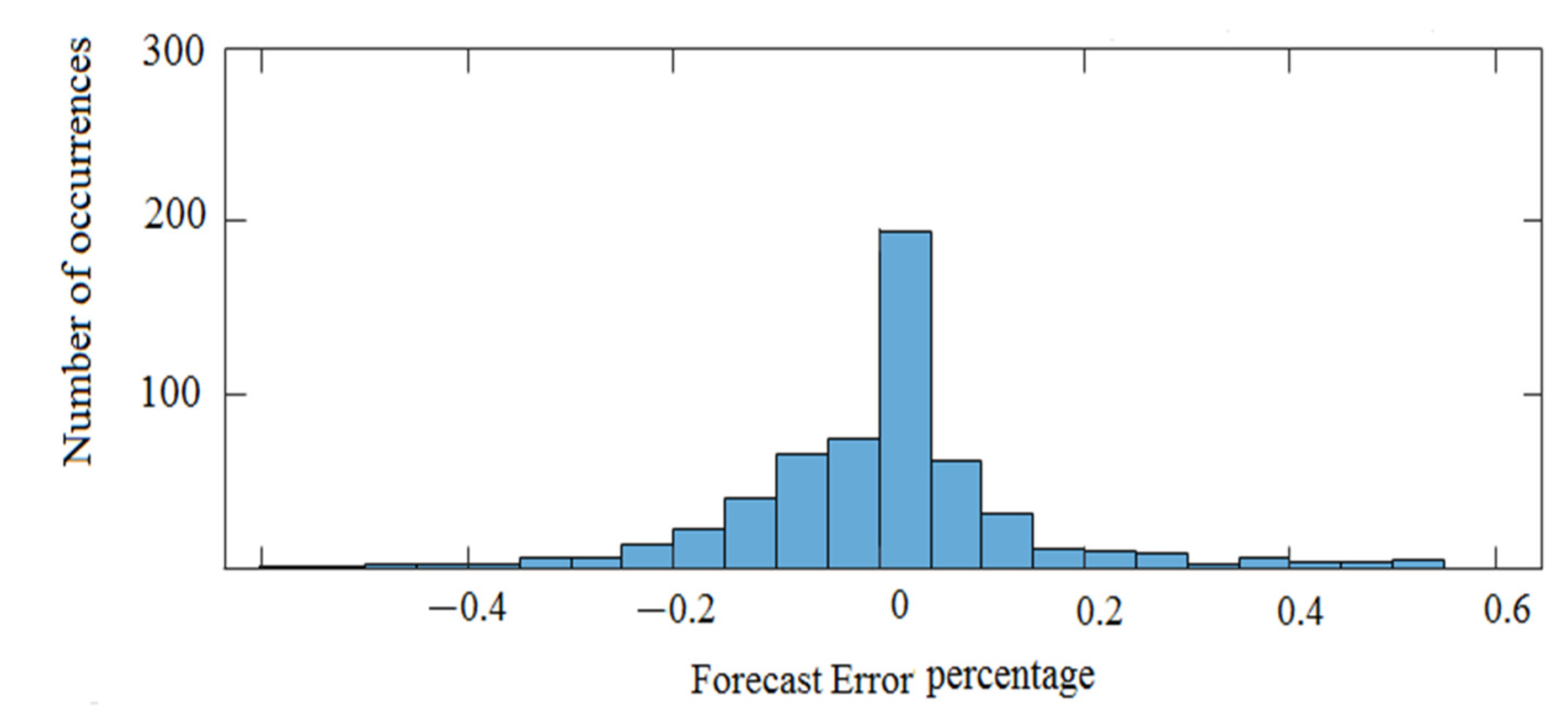
Table 6 presents the overall performance of all prediction models. In this section, the percentage of forecast error for ARIMAX, as an example, over one week of the PV system data, has been analysed by plotting the histogram of prediction error in Figure 21. Firstly, the values of forecast error were distributed within a wide range (−0.6 and 0.6). Secondly, the high number of forecast error percentages clustered around 0%, while many of the errors were distributed between −0.2% and 0.2%. Therefore, the normal distribution of the forecast error seems to accurately describe the ARIMAX model error by showing no bias distribution. In addition, this shows that it may be difficult to improve the performance of the forecast models any further, as the error centralised around zero. As previously discussed, the household demand and PV system profiles are volatile and less predictable compared to aggregated LV demands or MV demands. However, the forecast models in this paper are accurate compared to examples presented in the literature. For example, an ANN forecast model was presented by Bi et al. [46] to predict the power output of a PV system. The results show a 10.06% and 18.9% MAPE forecast error during sunny and rainy days, respectively. The high MAPE was mainly related to the type of exogenous variables used in the model. In [46], the high, low and average temperature values for similar days was used to generate the forecast profile. The average temperature over the day introduced less correlation with current demand compared to the hourly temperature, where normally the temperature changes from morning to midday to evening time. The differences between the actual temperature and average temperature will reflect demand consumption and PV output, as presented in Section 3. In this paper, the hourly temperature and historical data correlation were used to predict the PV profile.

5.3. Effect of Exogenous Variables on Forecast Models

In order to improve the performance of the forecast models and minimise the high error peaks, exogenous variables such as weather conditions have been used. In this paper, the impact of the exogenous variables in ANN and ARIMAX models has been evaluated by dividing the forecast models into sub-models as follows:

• Model A1: ARIMAX with two exogenous variables (${\mathrm{X}}_1$: Temperature and${ \mathrm{X}}_2$: Wind Speed).
• Model A2: ARIMAX with one exogenous variable (${\mathrm{X}}_1$: Temperature).
• Model A3: ARIMAX with one exogenous variable (${\mathrm{X}}_2$: Wind Speed).
• Model A4: ARIMA (2,1,2) model for the household and Madaba city demand and ARIMA (1,1,2) for PV output. The ARIMA model has been derived by removing the external variables term from the ARIMAX model.
• Model NN1: ANN with the following exogenous variables (${\mathrm{X}}_1$: Temperature, ${\mathrm{X}}_2$: Wind Speed, ${\mathrm{X}}_3:$Hour of the day, ${\mathrm{X}}_4$: Previous hour data, ${\mathrm{X}}_5$: Previous day data in same hour).
• Model NN2: ANN model without exogenous variables that is related to weather conditions and includes the following variables (${\mathrm{X}}_3:$Hour of the day, ${\mathrm{X}}_4$: Previous hour data, ${\mathrm{X}}_5$: Previous day data in same hour).
• Model NN3: ANN model without exogenous variables that is related to time series and seasonality and includes only the variables related to weather condition (${\mathrm{X}}_1$: Temperature, ${\mathrm{X}}_2$: Wind Speed).

In this section, the previous prediction models have been tested for predicting the PV power output (single household system) over the testing period.

Table 7. Overall performance of short-term forecasting models over testing days.

	Forecast Models
	Model A1	Model A2	Model A3	Model A4	Model NN1	Model NN2	Model NN3	ANN [47]	LSTM [47]
MAPE	7%	8.3%	10.1%	15.8%	6.2%	14.9%	19.7%	17.3%	24.%
RMSE	49.2 W	54.3 W	61.7 W	75.8 W	45.1 W	70.3 W	108.9 W	98.7 W	153.2 W

shows significant improvements in the MAPE and RMSE for all ARIMAX and ANN forecast models using the exogenous variables (weather conditions) compared to the ARIMA and ANN models that depend only on the time series correlation. The MAPE of NN1 model decreased by 5.6% compared to NN2. The RMSE values of Model A1 decreased by 21.6 W compared to Model A4. Overall, forecast models with the exogenous variables improve the prediction accuracy and exhibit large errors. This indicates, in the current PV system data set, that the exogenous variables in line with the historical data are recommended as inputs for the forecast model. Model A2 using only the temperature as exogenous variable and Model A1 (with two exogenous variables: wind speed and temperature) performed in a similar way with differences in accuracy of less than 1.3%. Furthermore, Table 5 shows that Model A2 is slightly more accurate compared to Model A3 with wind speed as exogenous variable. This indicates that temperature information has a more significant impact on the prediction performance than the wind speed for the PV system output forecast. Based on the analysis of the PV data set and performance of the forecast models, the prediction models require both wind speed and temperature as exogenous variables. On the other hand, one of these as exogenous variable can help to reduce the error peaks and the impact of outlier values. The results of Model A4 and Model NN2 show high forecast errors compared to all other models. This is mainly due to the high correlation between current demand and external variables (related to weather conditions) which are stronger and associated more with demands compared to times series autocorrelation at low voltage demand, with a high level of uncertainty. Weather conditions (as external variables) increase the ability to capture the chaining of demand behaviour at low voltage level in line with the seasonality and time series autocorrelation presented by Model A1 and Model NN1. However, Model NN3 employed only weather conditions (as external variables) without taking into account any time series autocorrelation or variables such as the time of the day or the previous load, which led to a high forecast error of 19.7% due to the weather conditions normally being fixed for different hours during the day. The forecast models NN1 and NN2, as ‘inelegant’ forecast models, outperformed the deep learning ANN model [47] and Long Short-Term Memory model (LSTM) [47]. The results of [47] in Table 7 are the average best results for ten householders.

5.4. Evaluating of the Importance of Designing a Rolling Load Forecast

In this paper, the proposed forecast models are extended to create a rolling demand forecast. The rolling forecast model aims to firstly predict the hourly household demand a day ahead, and then the forecast model will be updated after each time step. This procedure aims to recalculate and update the forecast profile for the following 24 h by using the new real-time measurements and forecast error. The rolling forecast model aims to minimise the forecast error compared to a fixed forecast model over one day.

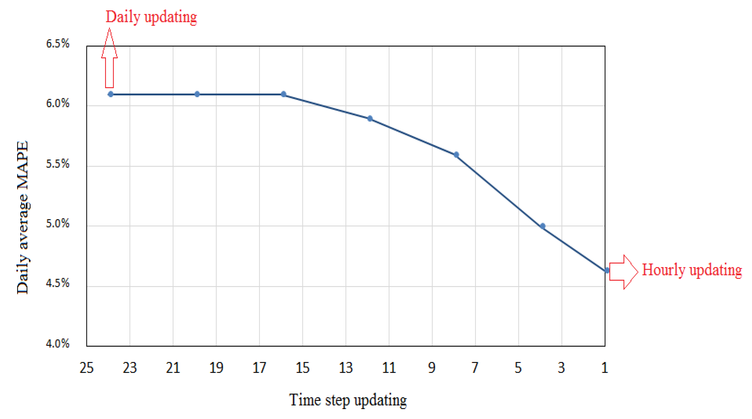
To assess the rolling forecast accuracy for the proposed forecast models, overall daily MAPE is presented in

Table 8. The daily mean absolute percentage error (MAPE) for the rolling and fixed models started from 1 October 2020.

	Traditional ANN		ARIMAX		ANN-GROM		Probabilistic-ARIMAX
	Rolling Forecast	Fixed Forecast	Rolling Forecast	Fixed Forecast	Rolling Forecast	Fixed Forecast	Rolling Forecast	Fixed Forecast
Day 1	4.2%	5.8%	5.9%	6.6%	3.1%	4.0%	4.3%	5.7%
Day 2	3.9%	4.1%	5.7%	7.1%	2.8%	3.9%	4.5%	5.9%
Day 3	4.8%	6.1%	5.3%	6.9%	3.3%	5.1%	4.2%	6.0%
Day 4	5.2%	7.3%	7.1%	8.6%	4.2%	5.3%	5.1%	6.8%
Day 5	5.4%	6.1%	6.7%	7.9%	4.5%	5.5%	5.4%	6.1%
Day 6	5.1%	8.7%	8.1%	9.3%	4.1%	6.2%	5.5%	7.2%
Day 7	3.8%	4.1%	3.8%	4.2%	2.9%	3.9%	4.0%	4.1%

. A comparison of the rolling (updating each time step) and fixed forecast models (updating with daily bases) of a single household demand over 7 days, as depicted in Table 8 and Figure 22, shows that prediction performance of the rolling model significantly improves compared to the fixed model. For example, on Day 4 the daily MAPE decreased from 7.3% to 5.2% for ANN and from 8.6% to 7.1% for ARIMAX. The minimum and maximum daily MAPE improvements in the rolling ANN-GROM forecast model was on Day 5 and Day 3, by 18% and 35.2%, respectively. In addition, the average daily MAPE over the testing period for the rolling ANN but with a different time updating schedule is presented in Figure 22. The hourly updating (rolling forecast) improves the overall daily MAPE by 28% compared to 12 h updating. The MAPE slightly improves (less than 3%) after 12-time step updating. This indicates that the updated measurements can help to increase the prediction model accuracy. However, the rolling process will increase the computational costs compared to fixed forecast.

5.5. Evaluating the Impact of Demand Disaggregation

In Section 1, the literature of load forecasting focused on a high and medium voltage level and, for low voltage level, focused on feeders’ demand (aggregations of smart meter data). In general, low voltage demand for individual users is much more stochastic and non-smooth than high and medium voltage level or aggregation low voltage demand level due to the high uncertainty in the demand profile. Nowadays, smart grid and micro-grid systems aim to concentrate on using distribution generation and individual user needs for more efficient energy management models and networks. Therefore, implementation of new intelligent methods and probabilistic forecasts is required to consider the high level of uncertainty based on the level of aggregation of smart meters [21]. For example, the authors in [21] used Recurrent Neural Network (RNN) to estimate the power and energy demand of low voltage applications as load disaggregation in order to achieve a more efficient energy management system.

Table 9. Overall performance of the proposed forecast models for demand disaggregation.

	Traditional ANN		ANN-GROM		Probabilistic-ARIMAX
	MAPE	RMSE	MAPE	RMSE	MAPE	RMSE
Single household demand	5.7%	30.1 W	3.4%	20.1 W	4.7%	28.1 W
Aggregation of ten household demand	4.9%	250.9 W	3.2%	190.5 W	4.5%	250.3 W
Madaba City	4.3%	860 kW	3.1%	620 kW	4.2%	845 kW

presented the forecast models’ results for three different level of aggregations: single household, aggregation of ten households’ demand (LV demand feeder), and small city (medium voltage). All forecast models performed more accurately with aggregated demand compared to single household demand. This is mainly related to the time series autocorrelations and correlation between the current demand and external variables which are stronger and more associated with aggregation demands, such as feeder and medium voltage level demand. For more explanation, larger demands (high and medium voltage levels and aggregation low voltage), which consist of aggregations of larger numbers of individual householders, increase the prominent regularities in daily, weekly and seasonal behaviour.

5.6. Evaluation of the Proposlaictc Forecast

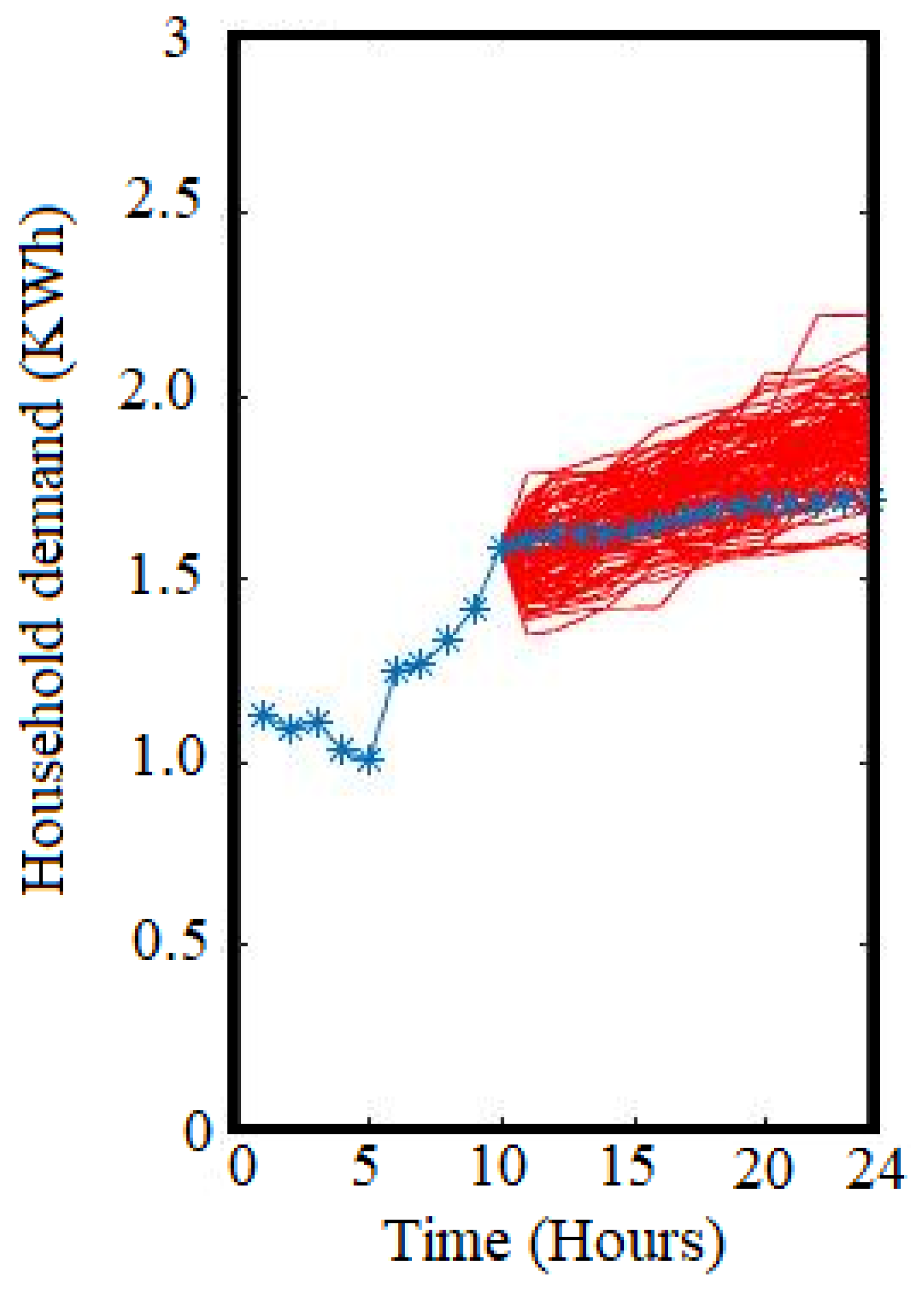
The ensemble forecast model is a common technique to create future power load scenarios and feed stochastic controllers with different input scenarios [31,38]. However, there are difficulties in comparing point forecasting model results such as ARIMAX and ANN to ensemble forecast scenarios, where these techniques are not directly comparable. The analysis of the ensemble forecast results in this section aims to show the significance of using different forecasting techniques when it is important to handle uncertainty in different engineering problems. In general, the forecast process can be repeated to generate 1000 to 10,000 scenarios. However, the more scenarios created, the higher the computational cost, but it will give more diversity of the power load to be captured. In Figure 23, an example of the simulated ensembles forecast model is presented. The scenarios of future single household demand $\hat{\mathrm{L}}\left(\mathrm{t}\right)$, are shown in red lines deviating closely around the actual demand values. However, the forecast errors get wider when increasing the horizon length in the forecast model due to the accumulation of forecast errors over each step, which also describes the high uncertainty at the end of the prediction horizon length.

6. Conclusions

The non-smooth and stochastic nature of household demand and PV power output, with no clear time series patterns compared to aggregate demand such as MV, increases the uncertainty levels and challenge of predicting LV applications. Therefore, an advanced prediction technique is required to minimise the impact of non-smooth demand behavior and reduce forecast error. In this paper, Probabilistic-ARIMAX and ANN-GROM forecast models have been developed and implemented to predict different LV applications and improve the performance of the prediction models by using exogenous variables, a new optimization method and a rolling forecast technique to forecast models. The proposed forecast models have been trained and tested by using real-time power grid data. The forecast model results show that the proposed prediction models with exogenous variables and a rolling forecast technique are effective at reducing forecast error. In particular, the ANN-GROM, for the given household demand data, has favourable results and outperforms the traditional ANN, ARIMAX and Probabilistic-ARIMAX. For example, the MAPE for ANN-GROM model improved by 41.2% for household demand forecast compared to the traditional ANN model and showed high ability to capture the chaining in disaggregation demands. In line with the benefits of forecast error reduction, it could also potentially understand LV application demand, and DNOs gain considerable technical and economic benefits from household demand and PV data analysis and this forecast model. In addition, using different optimization methods such as ELM to train the ANN forecast model will form part of our future work.

References

1. Klingler, A.-L.; Teichtmann, L. Impacts of a forecast-based operation strategy for grid-connected PV storage systems on profitability and the energy system. Sol. Energy 2017, 158, 861–868. [Google Scholar] [CrossRef]
2. Lee, C.-M.; Ko, C.-N. Short-Term Load Forecasting Using Adaptive Annealing Learning Algorithm Based Reinforcement Neural Network. Energies 2016, 9, 987. [Google Scholar] [CrossRef] [Green Version]
3. Bennett, C.J.; Stewart, R.A.; Lu, J.W. Forecasting low voltage distribution network demand profiles using a pattern recognition based expert system. Energy 2014, 67, 200–212. [Google Scholar] [CrossRef] [Green Version]
4. Deb, C.; Zhang, F.; Yang, J.; Lee, S.E.; Shah, K.W. A review on time series forecasting techniques for building energy consumption. Renew. Sustain. Energy Rev. 2017, 74, 902–924. [Google Scholar] [CrossRef]
5. Aneiros, G.; Vilar, J.; Raña, P. Short-term forecast of daily curves of electricity demand and price. Int. J. Electr. Power Energy Syst. 2016, 80, 96–108. [Google Scholar] [CrossRef]
6. Alasali, F.; Haben, S.; Becerra, V.; Holderbaum, W. Day-ahead industrial load forecasting for electric RTG cranes. J. Mod. Power Syst. Clean Energy 2018, 6, 223–234. [Google Scholar] [CrossRef] [Green Version]
7. Yogarajah, B.; Elankumaran, C.; Vigneswaran, R. Application of ARIMAX Model for Forecasting Paddy Production in Trincomalee District in Sri Lanka. In Proceedings of the 3rd International Conference at the South Eastern University of Sri Lanka, Oluvil, Sri Lanka, 6–7 July 2013. [Google Scholar]
8. Alfares, H.; Nazeeruddin, M. Electric load forecasting: Literature survey and of methods. Int. J. Syst. Sci. 2002, 33, 23–34. [Google Scholar] [CrossRef]
9. Chadsuthi, S.; Modchang, M.; Lenbury, Y.; Iamsirithaworn, S.; Triampo, W. Modeli-ng seasonal leptospirosis transmission and its association with rainfall and temperature in Thailand using time-series and ARIMAX analyses. Asian Pac. J. Trop. Med. 2012, 5, 539–546. [Google Scholar] [CrossRef] [Green Version]
10. Barak, S.; Sadegh, S.S. Forecasting energy consumption using ensemble ARIMA–ANFIS hybrid algorithm. Int. J. Electr. Power Energy Syst. 2016, 82, 92–104. [Google Scholar] [CrossRef] [Green Version]
11. Amini, M.H.; Kargarian, A.; Karabasoglu, O. ARIMA-based decoupled time series forecasting of electric vehicle charging demand for stochastic power system operation. Electr. Power Syst. Res. 2016, 140, 378–390. [Google Scholar] [CrossRef]
12. Hernandez, L.; Baladrón, C.; Aguiar, J.M.; Carro, B.; Sanchez-Esguevillas, A.J.; Lloret, J. Short-Term Load Forecasting for Microgrids Based on Artificial Neural Networks. Energies 2013, 6, 1385–1408. [Google Scholar] [CrossRef] [Green Version]
13. Yuan, S.; Kocaman, A.S.; Modi, V. Benefits of forecasting and energy storage in isolated grids with large wind penetration—The case of Sao Vicente. Renew. Energy 2017, 105, 167–174. [Google Scholar] [CrossRef]
14. Labidi, M.; Eynard, J.; Faugeroux, O.; Grieu, S. A new strategy based on power demand forecasting to the management of multi-energy district boilers equipped with hot water tanks. Appl. Therm. Eng. 2017, 113, 1366–1380. [Google Scholar] [CrossRef]
15. Wei, D.; Wang, J.; Ni, K.; Tang, G. Research and Application of a Novel Hybrid Model Based on a Deep Neural Network Combined with Fuzzy Time Series for Energy Forecasting. Energies 2019, 12, 3588. [Google Scholar] [CrossRef] [Green Version]
16. Hossain, M.; Mekhilef, S.; Danesh, M.; Olatomiwa, L.; Shamshirband, S. Application of extreme learning machine for short term output power forecasting of three grid-connected PV systems. J. Clean. Prod. 2017, 167, 395–405. [Google Scholar] [CrossRef]
17. Bessani, M.; Massignan, J.; Santos, T.; London, J., Jr.; Maciel, C. Multiple households very short-term load forecasting using Bayesian Networks. Elect. Power Syst. Res. 2020, 189, 106733. [Google Scholar] [CrossRef]
18. Wen, L.; Zhou, K.; Yang, S. Load demand forecasting of residential buildings using a deep learning model. Electr. Power Syst. Res. 2020, 179, 106073. [Google Scholar] [CrossRef]
19. Grant, J.; Eltoukhy, M.; Asfour, S. Short-Term Electrical Peak Demand Forecasting in a Large Government Building Using Artificial Neural Networks. Energies 2014, 7, 1935–1953. [Google Scholar] [CrossRef] [Green Version]
20. Teo, T.T.; Logenthiran, T.; Woo, W.L. Forecasting of photovoltaic power using extreme learning machine. In Proceedings of the 2015 IEEE Innovative Smart Grid Technologies—Asia (ISGT ASIA), Bangkok, Thailand, 3–6 November 2015; Institute of Electrical and Electronics Engineers (IEEE): New York, NY, USA, 2016; pp. 1–6. [Google Scholar]
21. Quek, Y.T.; Woo, W.L.; Logenthiran, T. Load Disaggregation Using One-Directional Convolutional Stacked Long Short-Term Memory Recurrent Neural Network. IEEE Syst. J. 2019, 14, 1395–1404. [Google Scholar] [CrossRef]
22. Wang, Y.; Hug, G.; Liu, Z.; Zhang, N. Modeling load forecast uncertainty using generative adversarial networks. Electr. Power Syst. Res. 2020, 189, 106732. [Google Scholar] [CrossRef]
23. Alasali, F.; Nusair, K.; Alhmoud, L.; Zarour, E. Impact of the COVID-19 Pandemic on Electricity Demand and Load Forecasting. Sustainability 2021, 13, 1435. [Google Scholar] [CrossRef]
24. Badran, I.; El-Zayyat, H.; Halasa, G. Short-Term and Medium-Term Load Forecasting for Jordan’s Power System. Am. J. Appl. Sci. 2008, 5, 763–768. [Google Scholar] [CrossRef]
25. Arfoa, A.A. Long-Term Load Forecasting of Southern Governorates of Jordan Distribution Electric System. Energy Power Eng. 2015, 7, 242–253. [Google Scholar] [CrossRef] [Green Version]
26. AbuAl-Foul, B. Forecasting Energy Demand in Jordan Using Artificial Neural Networks. Top. Middle East. Afr. Econ. 2012, 14, 473–478. [Google Scholar]
27. Momani, M.; Alrousan, W.; Alqudah, A. Short-term load forecasting based on NARX and radial basis neural networks approaches for the Jordanian power grid. Jordan J. Electr. Eng. 2016, 2, 81–93. [Google Scholar]
28. Huang, N.; Lu, G.; Xu, D. A Permutation Importance-Based Feature Selection Method for Short-Term Electricity Load Forecasting Using Random Forest. Energies 2016, 9, 767. [Google Scholar] [CrossRef] [Green Version]
29. Alasali, F.; Haben, S.; Holderbaum, W. Energy management systems for a network of electrified cranes with energy storage. Int. J. Electr. Power Energy Syst. 2019, 106, 210–222. [Google Scholar] [CrossRef]
30. Feuerriegel, S.; Riedlinger, S.; Neumann, D. Predictive Analytics for Electricity Prices Using Feed-ins From Renewables. In Proceedings of the Twenty Second European Conference on Information Systems, Aviv, Israel, 9–11 June 2014. [Google Scholar]
31. Alasali, F.; Haben, S.; Becerra, V.; Holderbaum, W. Optimal Energy Management and MPC Strategies for Electrified RTG Cranes with Energy Storage Systems. Energies 2017, 10, 1598. [Google Scholar] [CrossRef] [Green Version]
32. Cui, H.; Peng, X. Short-term city electrical load forecasting with considering tempe-rature effects: An improved ARIMAX model. Math. Probl. Eng. 2015, 2015, 589374. [Google Scholar] [CrossRef] [Green Version]
33. Ziegel, E.R.; Box, G.; Jenkins, G.; Reinsel, G. Time Series Analysis, Forecasting, and Control. Technometrics 1995, 37, 238. [Google Scholar] [CrossRef]
34. Jalalkamali, A.; Moradi, M.; Moradi, N. Application of several artificial intelligence models and ARIMAX model for forecasting drought using the Standardized Precipitation Index. Int. J. Environ. Sci. Technol. 2015, 12, 1201–1210. [Google Scholar] [CrossRef] [Green Version]
35. Sun, M.; Li, J.; Gao, C.; Han, D. Identifying regime shifts in the US electricity market based on price fluctuations. Appl. Energy 2017, 194, 658–666. [Google Scholar] [CrossRef]
36. Lee, C.-W.; Lin, B.-Y. Application of Hybrid Quantum Tabu Search with Support Vector Regression (SVR) for Load Forecasting. Energies 2016, 9, 873. [Google Scholar] [CrossRef] [Green Version]
37. Yan, X.; Chowdhury, N.A. Mid-term electricity market clearing price forecasting utilizing hybrid support vector machine and auto-regressive moving average with external input. Int. J. Electr. Power Energy Syst. 2014, 63, 64–70. [Google Scholar] [CrossRef]
38. Montgomery, D.; Jennings, C.; Kulahchi, M. Introduction to Time Series Analysis and Forecasting—III; John Wiley and Sons: Hoboken, NJ, USA, 2014; ISBN 978-0-4 71-65397-4. [Google Scholar]
39. Taylor, J.W.; de Menezes, L.M.; McSharry, P.E. A comparison of univariate methods for forecasting electricity demand up to a day ahead. Int. J. Forecast. 2006, 22, 1–16. [Google Scholar] [CrossRef]
40. Bennett, C.; Stewart, R.A.; Lu, J. Autoregressive with Exogenous Variables and Neural Network Short-Term Load Forecast Models for Residential Low Voltage Distribution Networks. Energies 2014, 7, 2938–2960. [Google Scholar] [CrossRef]
41. Amjady, N.; Keynia, F. A New Neural Network Approach to Short Term Load Forecasting of Electrical Power Systems. Energies 2011, 4, 488–503. [Google Scholar] [CrossRef]
42. Ramos, D.; Faria, P.; Vale, Z.; Mourinho, J.; Correia, R. Industrial Facility Electricity Consumption Forecast Using Artificial Neural Networks and Incremental Learning. Energies 2020, 13, 4774. [Google Scholar] [CrossRef]
43. Nusair, K.; Alasali, F. Optimal Power Flow Management System for a Power Network with Stochastic Renewable Energy Resources using Golden Ratio Optimization Method. Energies 2020, 13, 3671. [Google Scholar] [CrossRef]
44. Hyndman, R.; Athanasopoulos, G. Forecasting: Principles and Practice. ISBN 978-0-9875071-0-5, Printed Edition 2014. Available online: https://www.otexts.org/fpp (accessed on 20 January 2021).
45. Munkhammara, J.; Widna, J.; Rydnb, J. On a probability distribution model comb-ining household power consumption, electric vehicle home-charging and photovoltaic power production. Appl. Energy 2015, 142, 135–143. [Google Scholar] [CrossRef]
46. Ding, M.; Wang, L.; Bi, R. An ANN-based Approach for Forecasting the Power Output of Photovoltaic System. Procedia Environ. Sci. 2011, 11, 1308–1315. [Google Scholar] [CrossRef] [Green Version]
47. Acharya, S.K.; Wi, Y.-M.; Lee, J. Short-Term Load Forecasting for a Single Household Based on Convolution Neural Networks Using Data Augmentation. Energies 2019, 12, 3560. [Google Scholar] [CrossRef] [Green Version]
Figure 1. The PV installed at the house, Jordan.
Energies 14 02151 g001
Figure 2. 3D Sketch for the photo-voltaic (PV) panel.
Energies 14 02151 g002
Figure 3. An example for a single household PV system output (House 5) over one week with sunny day.
Energies 14 02151 g003
Figure 4. The ten household PV system output curves for a typical sunny day (22 August 2019).
Energies 14 02151 g004
Figure 5. An example for a single household PV system output (House 7) over one week with unclear (cloudy) weather.
Energies 14 02151 g005
Figure 6. Partial Autocorrelation Function (PACF) plot for household PV output system within unclear sky days.
Energies 14 02151 g006
Figure 7. Illustration of distribution of: (a) household demand and temperature (b) PV system output and temperature in a 2D histogram.
Energies 14 02151 g007
Figure 8. Scatter plot of hourly demand vs. temperature in Jordan (Madaba).
Energies 14 02151 g008
Figure 9. Distribution and classification of hourly household demand.
Energies 14 02151 g009
Figure 10. Distribution and classification of hourly household demand.
Energies 14 02151 g010
Figure 11. Cluster analysis for total daily demand at Madaba city depending on days of the week.
Energies 14 02151 g011
Figure 12. Box plot of hourly household demand over six weeks starting from 1 January 2019.
Energies 14 02151 g012
Figure 13. Breakdown of hourly demand distribution by day type.
Energies 14 02151 g013
Figure 14. PACF plot for household demand for two-week time lags.
Energies 14 02151 g014
Figure 15. General schematic of the short-term load forecasting procedure implemented in this article.
Energies 14 02151 g015
Figure 16. Methodology of the Autoregressive Integrated Moving Average (ARIMA) and ARIMAX forecasting models.
Energies 14 02151 g016
Figure 17. The structure of typical artificial neuron processing in a neural network (NN) unit.
Energies 14 02151 g017
Figure 18. The methodology of the Artificial Neural Network (ANN) forecasting model.
Energies 14 02151 g018
Figure 19. An example of actual and forecast household demand profile results.
Energies 14 02151 g019
Figure 20. An example of actual and forecast net demand profile.
Energies 14 02151 g020
Figure 21. Illustration of prediction error in a histogram distribution.
Energies 14 02151 g021
Figure 22. Average of daily MAPE of rolling forecast model with different time step updating.
Energies 14 02151 g022
Figure 23. An example of the ensemble forecasts for household demand.
Energies 14 02151 g023