On Optimistic and Pessimistic Bilevel Optimization Models for Demand Response Management

Abstract

This paper investigates bilevel optimization models for demand response management, and highlights the often overlooked consequences of a common modeling assumption in the field. That is, the overwhelming majority of existing research deals with the so-called optimistic variant of the problem where, in case of multiple optimal consumption schedules for a consumer (follower), the consumer chooses an optimal schedule that is the most favorable for the electricity retailer (leader). However, this assumption is usually illegitimate in practice; as a result, consumers may easily deviate from their expected behavior during realization, and the retailer suffers significant losses. One way out is to solve the pessimistic variant instead, where the retailer prepares for the least favorable optimal responses from the consumers. The main contribution of the paper is an exact procedure for solving the pessimistic variant of the problem. First, key properties of optimal solutions are formally proven and efficiently solvable special cases are identified. Then, a detailed investigation of the optimistic and pessimistic variants of the problem is presented. It is demonstrated that the set of optimal consumption schedules typically contains various responses that are equal for the follower, but bring radically different profits for the leader. The main procedure for solving the pessimistic variant reduces the problem to solving the optimistic variant with slightly perturbed problem data. A numerical case study shows that the optimistic solution may perform poorly in practice, while the pessimistic solution gives very close to the highest profit that can be achieved theoretically. To the best of the authors’ knowledge, this paper is the first to propose an exact solution approach for the pessimistic variant of the problem.

1. Introduction

Stackelberg game models and the corresponding bilevel programming solution approaches for demand response management have received considerable attention recently. When focusing on the operational level, most models capture the interplay of an electricity retailer, who is the leader in the Stackelberg game, and its multiple consumers, who act as the followers. In the sequential game, the leader decides first on the electricity tariff or some other incentives, whereas the followers respond to the tariff by scheduling their loads accordingly. Stackelberg game models assume that the load response is calculated by solving an optimization problem, with the tariff as the parameter, to optimality. Numerous such approaches have been published, including models with deferrable or curtailable loads, batteries, electric vehicles (EVs), etc. [1,2,3,4,5].

In this paper, it is argued that despite the remarkable results, an important detail is frequently overlooked: the followers often have a large set of optimal solutions to their problems, and the selection of the response from this set is not defined properly. Moreover, different optimal solutions for the follower may bring radically different benefits for the leader. In bilevel optimization, the optimistic assumption states that the followers select their optimal solution that is the most favorable for the leader. In contrast, the pessimistic variant deals with the case where the followers return their least favorable optimal response to the leader, and hence, it safeguards from potential losses due to an unexpected selection. Most previous approaches in the literature implicitly make the optimistic assumption, although this assumption can hardly be enforced in practice. In this paper, the difference between the two variants of the bilevel problem is highlighted. Then, to the best of the authors’ knowledge, the first efficient exact solution approach for the pessimistic variant of a bilevel electricity tariff optimization problem in the literature is introduced. Moreover, it is shown that in most cases, the profit of the leader in the pessimistic variant can approach the profit that can be achieved in the optimistic variant.

It is important to emphasize at this point the difference between bilevel optimization as a mathematical modeling and solution approach, and hierarchical modeling techniques in general. Bilevel optimization [6] applies formal mathematical techniques to characterize and find the equilibrium in game-theoretical decision situations with two fully rational parties with given constraints and objectives, and a well-defined serial decision workflow. This is different from generic hierarchical modeling techniques that analyze the interplay of two or more decision makers, typically by solving the problems faced by the individual parties one by one, and constructing the overall outcome by assuming some coordination mechanism between them, often using simulation techniques; see, e.g., [7]. This paper considers bilevel optimization strictly in the former sense.

Main results. On the one hand, this paper proves formal properties of the optimal solutions of a bilevel tariff optimization problem, both for the easily tractable single-consumer special case, and the computationally hard general case with an arbitrary number of consumers. The main implication of these results is the reduction of the pessimistic variant to the optimistic one by perturbing the problem data and also the optimal price vector, which also results in the first efficient solution approach for the pessimistic variant. On the other hand, a numerical case study is presented that demonstrates that solving the optimistic problem may directly cause a significant loss of profit for the retailer if the consumers do not choose their optimal solution as expected.

Structure of the paper. After a brief literature review in Section 2, the bilevel electricity tariff optimization problem is defined formally in Section 3. Some general observations are presented in Section 4. In Section 5, a special case with one consumer only is studied. The general optimistic variant is treated in Section 6.1, and the pessimistic one in Section 6.2. An experimental evaluation is presented in Section 7, and the paper concludes in Section 8.

2. Literature Review

Introduced by the seminal paper of Bracken and McGill [8], bilevel optimization has become a field rich in deep theoretical results and with many practical applications; see, e.g., Bard [9], Dempe [6], and Colson et al. [10]. One of the central questions is expressing the optimality of the followers’ solutions in mathematical programming formulations. To this end, Karush–Kuhn–Tucker (KKT) necessary optimality conditions, or the Fritz John necessary optimality conditions, value functions, or penalty functions can be used [11,12,13,14,15,16].

As for the methods, the optimistic or strong bilevel optimization problem appears to be easier to solve than the pessimistic or weak bilevel problem in general; see, e.g., [17]. Most approaches reduce the strong bilevel optimization problem to a single-level problem by expressing the optimality of the lower-level solution by using one of the techniques mentioned above and then applying some non-linear programming methods for solving the resulting formulation [18]. There are many results for special cases. The linear bilevel programming problem, in which all constraints and objective functions are linear, is well understood; see, e.g., Ben-Ayed [19] and Dempe [6]. Lozano and Smith [20] described an exact method for nonlinear bilevel optimization problems, in which the leader has only integer variables, while the follower can have both integer and continuous variables. The constraints and the objective functions can be nonlinear, but all constraints are separable in terms of the leader and follower variables. They used a value function-based problem formulation in their enumeration procedure, and they extended it to the pessimistic problem as well. Since the leader’s variables can take only discrete values, an optimal solution always exists, provided the problem is feasible. Brotcorne et al. [21] studied a concrete application in which the leader sets freight tariffs on the arcs of a traffic network, and the follower aims at minimizing its transportation costs while satisfying transportation demands. Both objective functions are non-linear, but all constraints are linear. The authors proposed heuristics to obtain good solutions.

As for the weak variant, Loridan and Morgan [22], approximated the optimal solution by solving a sequence of strong bilevel optimization problems. Wiesemann et al. [23] provided an in-depth study of the pessimistic bilevel optimization problem under some restrictions. That is, the follower’s feasible set must be independent of the leader’s solution, and both the leader and the follower must have a compact set of feasible solutions. However, integrality of the variables at both levels is permitted. Under these assumptions, the optimal solution is approximated by solving a sequence of problems obtained by relaxing the value function of the follower by a decreasing sequence of additive constants. A new relaxation, based on the value function approach, was proposed by Zeng [17]. The approach works if an optimal solution exists, but the author also discussed some remedies when that is not the case, which may help sometimes. The crux of the method is to reduce the pessimistic bilevel optimization problem to solving one or two optimistic problems with a few additional constraints.

The electricity tariff optimization problem in scope and its various extensions have been investigated extensively in the electrical engineering community for demand response management in smart grids. This formulation is named the simple multi-period energy tariff optimization problem (SMETOP) in [24], where its NP-hardness is proved in case of multiple followers. Various papers address the extensions of the SMETOP, including generic piecewise linear, quadratic, or other non-linear follower utility functions [3,4]; battery storage at the follower [2], multi-energy systems [25]; or the heating, ventilation, and air-conditioning (HVAC) of buildings using a dedicated thermal model [26]. The typical solution approach is reformulating the bilevel problem into an equivalent single-level problem using the KKT conditions, eliminating non-linear terms, and then solving the model as a mixed-integer linear program (MILP) [3,5,27,28]. The possible alternatives include exploiting strong duality for the follower’s linear problem to convert the problem into a single-level quadratic program [2], or to use custom (meta-)heuristics to keep the computational load at bay [4,29,30]. A more detailed review on the solution approaches to bilevel programming models of demand response management can be found, e.g., in [2]. However, these approaches are applicable only to the optimistic (strong) variant of the bilevel problem. Applications of bilevel programming to energy networks are reviewed in [18]. Extensions to the stochastic case are presented, e.g., in [31,32].

The difference between the optimistic and the pessimistic variants of the bilevel optimization problem specifically in energy management is emphasized in [33]. The paper introduces the notion of a deceiving solution to denote the worst possible outcome for the leader if it applies the optimistic assumption but the follower deviates from the expected response, and similarly, the rewarding solution for the best possible outcome if the leader applies the pessimistic assumption but the follower decides for an unexpectedly favorable response. The paper applies a hybrid solution approach by combining a genetic algorithm and a MILP solver to find close-to-optimal solutions for both the optimistic and the pessimistic variants of the semivectorial bilevel problem in which the follower addresses the minimization of the bi-criteria composed of electricity cost and discomfort. However, the authors are not aware of efficient exact solution approaches to pessimistic bilevel optimization problems applicable to energy management.

3. Problem Definition

The paper investigates a bilevel electricity tariff optimization problem for demand response management as follows. In the bilevel problem, the leader is an electricity retailer who controls the electricity tariff (unit price) over a finite time horizon divided into T time periods, e.g., the 24 hours of a day. For each $t\in \{1,\dots ,T\}$, let $c_t$ be the wholesale market price of electricity, Q the average unit price, and $q_t^l$ and $q_t^u$ the lower and upper bounds, respectively, on the unit price of the electricity (to be determined by the leader) in time period t. There are m followers, the consumers, who buy electricity at the given prices over the time horizon in order to meet their demands. Follower i attributes some utility $u_{it}$ to consuming one unit of electricity in each time period t, its total demand over the time horizon is at least $D_i^l$ and at most $D_i^u$, and its consumption will be between $x_{it}^l$ and $x_{it}^u$ in each time period t.

It is noted that different loads of a household, which are scheduled independently (e.g., air conditioning, a washing machine, an EV charger, and other, inflexible loads) can be captured as separate consumers (followers) in the model. Likewise, a single consumer in the model can capture the ensemble of consumers with similar parameters in reality.

The profit of the leader, for a given price vector q, and the consumption vector x of the followers, are

$$p(q,x):=\sum _{t=1}^T\sum _{i=1}^m(q_t-c_t)x_{it}.$$

The leader wants to determine the unit prices $q_t$ in order to maximize its profit, that is,

$$\mathrm{Maximize}F\left(q\right)$$

(1)

subject to the constraints

$$\begin{array}{cc}\hfill & \frac{1}{T}\sum _{t=1}^T{q}_t\le Q\hfill \end{array}$$

(2)

$$\begin{array}{cc}\hfill & q_t^l\le q_t\le q_t^u,t=1,\dots ,T,\hfill \end{array}$$

(3)

where F is a function mapping the price vector to a profit value, and it can be evaluated after the followers solve their own optimization problems. F is defined after presenting the followers’ optimization problems. In fact, each follower i solves a continuous knapsack problem in which the objective function is parameterized by the price vector set by the leader:

$$\begin{array}{cc}\hfill \mathrm{Maximize}& \sum _{t=1}^T(u_{it}-q_t)x_{it}\hfill \end{array}$$

(4)

$$\begin{array}{cc}\hfill & D_i^l\le \sum _{t=1}^T{x}_{it}\le D_i^u\hfill \end{array}$$

(5)

$$\begin{array}{cc}\hfill & x_{it}^l\le x_{it}\le x_{it}^u,t=1,\dots ,T\hfill \end{array}$$

(6)

Assuming that (5)–(6) has a solution, each follower i has at least one optimal solution for any price vector q. Let $\Omega \left(q\right)\subset {\mathbb{R}}^{m\times T}$ denote the set of all optimal solutions of the followers. Observe that $\Omega \left(q\right)$ is never empty. If the followers have a unique optimal solution for q, i.e., $\Omega \left(q\right)$ contains only one element, then the leader’s profit is well defined for q. However, if $\Omega \left(q\right)$ has 2 or more members, then it is not clear in advance, which optimal solution would be returned by the followers. For instance, if $u_{it}-q_t=u_{i{t}^{\prime }}-q_{t^{\prime }}$, $x_{it}^u=x_{i{t}^{\prime }}^u$, and $x_{it}^l=x_{i{t}^{\prime }}^l$, for some $t\ne t^{\prime }$, and either $x_{it}$ or $x_{i{t}^{\prime }}$ can be set to upper bound in an optimal solution, then it is up to follower i which one to choose. However, its decision can significantly impact the profit of the leader. In the optimistic or strong variant of the bilevel problem, it is assumed that in cases with multiple optimal solutions, the followers return the one most favorable for the leader, i.e.,

$$F\left(q\right)=F_o\left(q\right):=\mathrm{Maximize}\{p(q,x^{☆}):x^{☆}\in \Omega \left(q\right)\}.$$

In contrast, in the pessimistic or weak variant, the leader prepares for the worst case; thus F(q), is computed using the least favorable optimal solution of the followers.

$$F\left(q\right)=F_p\left(q\right):=\mathrm{Minimize}\{p(q,x^{☆}):x^{☆}\in \Omega \left(q\right)\}.$$

As it will be shown shortly, the maximum of $F_p\left(q\right)$ may not be attained by any price vector q; hence, in the pessimistic variant, (1) is replaced by

$$\mathrm{Supremum}{F}_p\left(q\right).$$

(7)

The difference between the optimistic and pessimistic variants is illustrated by a small example.

Example 1

(Difference between the optimistic and the pessimistic variants). Suppose $T=2$, there is only one follower, the leaders’s average tariff is $Q=30$, and the follower’s desired consumption is $D^l=D^u=1$. Further data is depicted in

Table 1. Data for Example 1.

t	1	2
$c_t$	10	50
$q_t^l$	20	20
$q_t^u$	40	40
$u_t$	10	30
$x_t^l$	0	0
$x_t^u$	1	1

. In the optimistic variant of the problem, the optimal tariff vector is $q=(20,40)$ for which the best response is $x^o=(1,0)$ giving an objective function value of 10. In contrast, in the pessimistic variant of the problem, if $u_2-q_2\ge u_1-q_1$, the follower will load the second period with 1 unit of consumption, i.e., $x^p=(0,1)$, for which the leader’s objective function value is $q_2-50$. Since $20\le q_t\le 40$ and $q_1+q_2\le 60$, $u_1-q_1\le u_2-q_2$ for any feasible q. Thus the best option for the leader is $q_2=40$ (with arbitrary $q_1$), and its objective function value is $-10$ on $x^p=(0,1)$. Observe that with higher values of $c_2$, the loss of the leader can increase arbitrarily.

The next example shows that the pessimistic variant may not have an optimal solution, which justifies the supremum in (7).

Example 2

(No optimal solution for the pessimistic variant). Suppose $T=2$, there is only one follower, the leaders’s average tariff is $Q=40$, and $D^l=D^u=1$. Further data are depicted in

Table 2. Data for Example 2.

t	1	2
$c_t$	10	50
$q_t^l$	20	20
$q_t^u$	40	40
$u_t$	40	40
$x_t^l$	0	0
$x_t^u$	1	1

. The optimistic solution is $q=(40,40)$ and $x^o=(1,0)$, resulting in a profit of 30 for the leader. However, for $q=(40,40)$, the pessimistic answer would be $x^p=(0,1)$ for which the leader’s objective function value is $-10$. However, the leader can do much better by setting $q=(40-ϵ,40)$. Then $u-q=(ϵ,0)$; thus, the follower’s unique optimal solution is $x^p=(1,0)$ for which the leader’s objective function value is $30-ϵ$. Clearly, the supremum of the leader’s objective function value is 30, but it cannot be attained by any feasible solution.

4. Preliminaries

4.1. The Continuous Knapsack Problem

This section briefly overview the key properties of optimal solutions of the continuous knapsack problem as follows:

$$\begin{array}{cc}\hfill \mathrm{Maximize}& \sum _{t=1}^T{w}_t{x}_t\hfill \\ \hfill & D^l\le \sum _{t=1}^T{x}_t\le D^u\hfill \\ \hfill & x_t^l\le x_t\le x_t^u,t=1,\dots ,T,\hfill \end{array}$$

(8)

where $0\le x_t^l<x_t^u$ for all t. Note that the $w_t$ are not restricted in sign.

The continuous knapsack problem (8) admits a feasible solution if and only if ${\sum }_{t\in \left[T\right]}{x}_t^l\le D^u\le {\sum }_{t\in \left[T\right]}{x}_t^u$. When feasible, it always has a finite optimum, since all variables are bounded. Without loss of generality, $D^l\ge {\sum }_{t\in \left[T\right]}{x}_t^l$.

Proposition 1.

Suppose the continuous knapsack problem (8) admits a feasible solution. Then it has an optimal solution $x^{☆}$ of the following structure:

1. 

$x_t^{*}=x_t^l$ for $t\in L$, $x_t^{*}=x_t^u$ for $t\in U$;

2. 

$x_p^{*}\in \{x_p^l,x_p^u,D_p^l-{\sum }_{t\in L\cup U}{x}_t^{*},D_p^u-{\sum }_{t\in L\cup U}{x}_t^{*}\}$.

where $L\cup P\cup U$ is a partitioning of $\left[T\right]$ such that $P=\left\{p\right\}$ for some $p\in \left[T\right]$, $w_t\ge w_p$ for $t\in U$, and $w_t\le w_p$ for $t\in L$. Moreover, such a partitioning can be computed in $O(TlogT)$ time by determining a permutation π such that $w_{\pi \left(t\right)}\ge w_{\pi (t+1)}$ for $t=1,\dots ,T-1$.

4.2. General Properties of Optimal Solutions

Firstly, observe that without loss of generality, the lower bounds on the prices can be assumed to be 0.

Proposition 2.

If $q_t^l>0$, then an equivalent problem can be derived by setting

• $u_{it}:=u_{it}-q_t^l$ for $i=1,\dots ,m$;
• $c_t:=c_t-q_t^l$;
• $Q:=Q-q_t^l/T$;
• $q_t^u:=q_t^u-q_t^l$;
• $q_t^l:=0$.

Proof. 

Let ${\tilde{q}}_t=q_t-q_t^l$, while ${\tilde{q}}_{\tau }=q_{\tau }$ for $\tau \in \left[T\right]\setminus \left\{t\right\}$. Substituting $q_t$ with ${\tilde{q}}_t+q_t^l$ in (1)–(3) + (4)–(6) yields a formulation satisfying the properties of the statement. □

From now on, the following assumption is made:

Assumption 1.

$q_t^l=0$ for all $t\in \left[T\right]$, $Q>0$, and ${\sum }_{t=1}^T{q}_t^u\ge QT$.

The minimum consumption of each follower i is at least ${\sum }_{t=1}^T{x}_{it}^l$, while the maximum consumption is at most ${\sum }_{t=1}^T{x}_{it}^u$. Moreover, if $D_i^u={\sum }_{t=1}^T{x}_{it}^l$, then the follower i has a unique optimal solution, which is independent of q. Hence, without loss of generality, the following assumption also holds:

Assumption 2.

$D_i^l\ge {\sum }_{t=1}^T{x}_{it}^l$, and ${\sum }_{t=1}^T{x}_{it}^l<D_i^u\le {\sum }_{t=1}^T{x}_{it}^u$ for each i.

Now, an easy observation can be made about the leader’s optimal price vector, which is valid in the optimistic and in the pessimistic variant of the bilevel tariff optimization problem.

Proposition 3.

Let $(q^{☆},x^{☆})$ be an optimal solution for (1)–(3) + (4)–(6) such that ${\sum }_{t=1}^T{\sum }_{i=1}^m{x}_{it}^{☆}>0$. Then either $q_t^{☆}=q_t^u$ for some $t\in \left[T\right]$, or ${\sum }_{t=1}^T{q}_t^{☆}=QT$.

Proof. 

Suppose $q^{☆}$ does not satisfy the conditions of the statement. Then for $ϵ>0$ sufficiently small, the price vector $\tilde{q}=(q_1^{☆}+ϵ,\dots ,q_T^{☆}+ϵ)$ is feasible, and induces the same partitioning of the time periods as $q^{☆}$ for each follower i; cf. Proposition 1. Hence $(\tilde{q},x^{☆})$ constitutes a feasible solution for (1)–(3) + (4)–(6), and

$$\sum _{t=1}^T({\tilde{q}}_t-c_t)\sum _{i=1}^m{x}_{it}^{☆}=\sum _{t=1}^T(q_t^{☆}-c_t)\sum _{i=1}^m{x}_{it}^{☆}+ϵ\sum _{t=1}^T\sum _{i=1}^m{x}_{it}^{☆}>\sum _{t=1}^T(q_t^{☆}-c_t)\sum _{i=1}^m{x}_{it}^{☆},$$

where the last inequality follows from the assumption of the theorem. However, it follows that $(x^{☆},q^{☆})$ is not an optimal solution, a contradiction. □

5. Polynomially Solvable Special Cases with One Consumer Only

This section investigates the one-consumer special case ($m=1$), and under some further restrictions, polynomial time algorithms are provided for solving the optimistic and pessimistic variants as well.

Throughout this section, it is assumed that the prices are unbounded; i.e., $q_t^u=\infty$ for all t. In fact, by (2), it may equivalently be assumed that $q_t^u=QT$ for all t. Further on, some assumptions on regularity are introduced in the next section.

Firstly, the optimistic variant is discussed in Section 5.1, and the pessimistic one in Section 5.2.

5.1. The Optimistic Variant

Let us assume that $D^l=D^u$, and let D denote the common value. The case with $D^l<D^u$ will be discussed later.

Definition 1.

A price vector q is feasible if it satisfies (2) and (3).

Definition 2.

If $D=D^l=D^u$, then a time period $t\in \left[T\right]$ is regular, if

$$x_t^l<\frac{D}{T}<x_t^u.$$

Observation 1.

If there is at least one regular time period, then $D>0$.

Definition 3.

From now on, an optimal solution $(q^{☆},x^{☆})$ of (1)–(3) + (4)–(6) is called non-degenerate if $q_t^{☆}>0$ for all $t\in \left[T\right]$.

In the following results, it is assumed that $x^{☆}$ is an optimal solution of the continuous knapsack problem (8) for weights $w_t=u_t-q_t^{☆}$, and it respects the conditions of Proposition 1 for some partitioning $L\cup P\cup U$ of $\left[T\right]$, where $P=\left\{p\right\}$.

Lemma 1.

Assume (1)–(3) + (4)–(6) admits a non-degenerate optimal solution $(q^{☆},x^{☆})$, and suppose $t\in L$ is a regular time period. Then

$$u_t-q_t^{☆}=u_p-q_p^{☆}.$$

Proof. 

Let $(q^{☆},x^{☆})$ be a non-degenerate optimal solution of (1)–(3) + (4)–(6) such that $u_t-q_t^{☆}<u_p-q_p^{☆}$. Let

$$ϵ=min\{u_p-q_p^{☆}-(u_t-q_t^{☆}),q_t^{☆}\}.$$

Define a new price vector

$$\tilde{q}=\left(q_1^{☆}+\frac{ϵ}{T},\dots ,q_t^{☆}-ϵ+\frac{ϵ}{T},\dots ,q_T^{☆}+\frac{ϵ}{T}\right).$$

Then $\tilde{q}$ is a non-degenerate feasible solution of (1)–(3). Moreover, $x^{☆}$ is an optimal solution of the continuous knapsack problem (8) with weights ${\tilde{w}}_t=u_t-{\tilde{q}}_t$, as it satisfies the conditions of Proposition 1 for the same partitioning $L\cup P\cup U$ of $\left[T\right]$. However, the objective value (1) changes by

$$-ϵ·x_t^l+\frac{ϵ}{T}D.$$

Due to the regularity assumption

$$x_t^l<\frac{D}{T},$$

the change in the objective value is positive:

$$-ϵ·\left(x_t^l-\frac{D}{T}\right)>0$$

which contradicts the optimality of $(q^{☆},x^{☆})$. □

Lemma 2.

Assume (1)–(3) + (4)–(6) admits a non-degenerate optimal solution $(q^{☆},x^{☆})$, and suppose $t\in U$ is a regular time period. Then

$$u_t-q_t^{☆}=u_p-q_p^{☆}.$$

Proof. 

(sketch) Analogous to that of Lemma 1. It is only mentioned that in this case

$$\tilde{q}=\left(q_1^{☆}-\frac{ϵ}{T},\dots ,q_t^{☆}+ϵ-\frac{ϵ}{T},\dots ,q_T^{☆}-\frac{ϵ}{T}\right).$$

The rest follows from the regularity assumption, i.e., $D/T<x_t^u$. □

Lemma 3.

Suppose all time periods are regular, and (1)–(3) + (4)–(6) admits a non-degenerate optimal solution $(q^{☆},x^{☆})$. Then

$$u_{\tau }-q_{\tau }^{☆}=\sum _{t\in \left[T\right]}\frac{u_t}{T}-Q,\tau =1\dots ,T.$$

Proof. 

Since $u_t-q_t^{☆}=u_p-q_p^{☆}$ for all $t\in \left[T\right]$ by Lemmas 1 and 2, it holds for any $\tau \in \left[T\right]$ that

$$T(u_{\tau }-q_{\tau }^{☆})=\sum _{t\in \left[T\right]}{u}_t-\sum _{t\in \left[T\right]}{q}_t^{☆}=\sum _{t\in \left[T\right]}{u}_t-Q·T,$$

where the second equation follows from Proposition 3, since ${\sum }_{t=1}^T{x}_t^{☆}=D>0$, as each time period is regular. □

Now, a necessary and sufficient condition is provided for the existence of a non-degenerate optimal solution. Let $u_{min}={min}_{t\in \left[T\right]}{u}_t$.

Theorem 1.

Assume that all time periods are regular. The bilevel tariff optimization problem (1)–(3) + (4)–(6) admits a non-degenerate optimal solution if and only if $Q-(1/T){\sum }_{t\in \left[T\right]}{u}_t+u_{min}>0$.

Proof. 

First suppose (1)–(3) + (4)–(6) admits a non-degenerate optimal solution $(q^{☆},x^{☆})$. Then by Lemma 3, $q_t^{☆}=u_t-(1/T){\sum }_{\tau \in \left[T\right]}{u}_{\tau }+Q$, and thus $u_t-(1/T){\sum }_{\tau \in \left[T\right]}{u}_{\tau }+Q>0$ for all $t\in \left[T\right]$, and in particular $u_{min}-(1/T){\sum }_{\tau \in \left[T\right]}{u}_{\tau }+Q>0$.

In order the prove the converse direction, let us relax the bound constraints () for the $q_t$ variables, i.e., $-\infty <q_t<\infty$. Note that this relaxation permits unbounded optimum value for the leader. However, as it is shown below, this is not the case. Fix some feasible price vector $q^{☆}$, and let $x^{☆}$ be the corresponding optimal solution of the follower respecting the partitioning $L\cup P\cup U$ of $\left[T\right]$ given by Proposition 1. If ${\sum }_{t=1}^T{q}_t^{☆}<QT$, then while increasing all coordinates of $q^{☆}$ by the same value, the follower’s solution $x^{☆}$ remains optimal, and the profit of the leader increases. Thus, without loss of generality, ${\sum }_{t=1}^T{q}_t^{☆}=QT$. Suppose $P=\left\{p\right\}$ in the partitioning. If $q^{☆}$ fails to satisfy $u_t-q_t^{☆}=u_p-q_p^{☆}$ for some $t\in \left[T\right]$, then almost the same transformations can be applied as in Lemmas 1 and 2 to conclude that the leader’s objective function value can be improved:

• If $u_t-q_t^{☆}<u_p-q_p^{☆}$, then $t\in L$, and $q_t^{☆}$ is decreased by $ϵ-ϵ/T$, while $q_{\tau }^{☆}$ is increased by $ϵ/T$ for all $\tau \ne t$, where $ϵ=u_p-q_p^{☆}-(u_t-q_t^{☆})$.
• If $u_t-q_t^{☆}>u_p-q_p^{☆}$, then $t\in U$, and $q_t^{☆}$ is increased by $ϵ-ϵ/T$, while $q_{\tau }^{☆}$ increases by $ϵ/T$ for all $\tau \ne t$, where $ϵ=u_t-q_t^{☆}-(u_p-q_p^{☆})$.

In either case, $x^{☆}$ remains optimal for the resulting price vector, and the leader’s objective function value strictly increases.

By repeating this transformation, a solution $\widehat{q}$ of the relaxed problem is derived such that $u_t-{\widehat{q}}_t=u_p-{\widehat{q}}_p$ for all $t\in \left[T\right]$, while $x^{☆}$ remains optimal for $\widehat{q}$. However, $\widehat{q}$ satisfies ${\widehat{q}}_t=u_t-(1/T){\sum }_{\tau \in \left[T\right]}{u}_{\tau }+Q$ for all $t\in \left[T\right]$ (see the proof of Lemma 3). Consequently, if $u_{min}-(1/T){\sum }_{\tau \in \left[T\right]}{u}_{\tau }+Q>0$, then $u_t-(1/T){\sum }_{\tau \in \left[T\right]}{u}_{\tau }+Q>0$ for all $t\in \left[T\right]$. Hence, $\widehat{q}$ is a non-degenerate feasible solution for the leader and $(x^{☆},\widehat{q})$ has a strictly greater objective function value than $(x^{☆},q^{☆})$. Since the above argument applies to any vector $q^{☆}$ with finite coordinates only, it can be deduced that $u_{min}-(1/T){\sum }_{\tau \in \left[T\right]}{u}_{\tau }+Q>0$ implies that there exists a non-degenerate optimal solution of the bilevel tariff optimization problem. □

Theorem 2.

Suppose $D^l=D^u$, all time periods are regular, and (1)–(3) + (4)–(6) admits a non-degenerate optimal solution $(q^{☆},x^{☆})$. Then

$$q_{\tau }^{☆}=u_{\tau }-\frac{1}{T}\sum _{t\in \left[T\right]}{u}_t+Q,\tau =1,\dots ,T.$$

Moreover, the optimal consumptions $x^{☆}$ can be obtained by solving the continuous knapsack problem:

$$\begin{array}{cc}\hfill \mathrm{Maximize}& \sum _{t=1}^T(q_t^{☆}-c_t)x_t\hfill \\ \hfill & \sum _{t=1}^T{x}_t=D\hfill \\ \hfill & x_t^l\le x_t\le x_t^u,t=1,\dots ,T.\hfill \end{array}$$

Proof. 

The first part of the statement follows from Lemma 3, and the second part from the optimality of $q^{☆}$. □

Note that Theorem 2 yields an optimal solution for the optimistic variant of the bilevel tariff optimization problem. Then, $x^{☆}$ can be computed by using Proposition 1.

Now, consider the more general case when $D^l<D^u$.

Definition 4.

If $D^l<D^u$, then a time period $t\in \left[T\right]$ is regular if

$$x_t^l<\frac{D^l}{T}and\frac{D^u}{T}<x_t^u.$$

Theorem 3.

Suppose $D^l<D^u$, all time periods are regular, and (1)–(3) + (4)–(6) admits a non-degenerate optimal solution $(q^{☆},x^{☆})$. Then $x^{☆}$ satisfies

$$D^l\le \sum _{t\in \left[T\right]}{x}_t^{☆}\left\{\begin{array}{cc}=D^u\hfill & \mathrm{if}(1/T)\sum _{t\in \left[T\right]}{u}_t-Q>0,\hfill \\ \le D^u\hfill & \mathrm{if}(1/T)\sum _{t\in \left[T\right]}{u}_t-Q=0,\hfill \\ =D^l\hfill & \mathrm{if}(1/T)\sum _{t\in \left[T\right]}{u}_t-Q<0.\hfill \end{array}\right.$$

Proof. 

The first inequality follows from the feasibility of $x^{☆}$. Define $q_t^{☆}$ as in Theorem 1. Then $u_t-q_t^{☆}=(1/T){\sum }_{\tau \in \left[T\right]}{u}_{\tau }-Q$ for all $t\in \left[T\right]$; i.e., the objective function coefficient of the follower is the same in all time periods. Hence, the follower’s optimal solution is chosen based on the leader’s objective function ${\sum }_{t\in \left[T\right]}(q_t^{☆}-c_t)x_t$. That is, the follower solves (8) with

Clearly, if $(1/T){\sum }_{\tau \in \left[T\right]}{u}_{\tau }-Q<0$, then in any optimal solution of the follower, the periods are loaded to the least possible extent until $D^l$ is reached, since all objective function coefficients (of the follower) are negative. Therefore, since the follower chooses an optimal solution which maximizes the leader’s objective function value, the follower solves (8) with cost vector $w_t:=q_t^{☆}-c_t$ for $t\in \left[T\right]$, while $D^u$ is replaced with $D^l$. Analogously, if $(1/T){\sum }_{\tau \in \left[T\right]}{u}_{\tau }-Q>0$, then in any optimal solution of the follower, the periods are loaded to the maximal possible amount until $D^u$ is reached. Therefore, the follower solves (8) with cost vector $w_t:=q_t^{☆}-c_t$ for $t\in \left[T\right]$, while $D^l$ is replaced with $D^u$.

Finally, if $(1/T){\sum }_{\tau \in \left[T\right]}{u}_{\tau }-Q=0$, then the follower chooses its optimal solution solely by considering the objective function of the leader—namely, it solves the fractional knapsack problem (8) with weights $w_t:=q_t^{☆}-c_t$. The result follows from Proposition 1. □

5.2. The Pessimistic Variant

Under the conditions of Theorem 2, the optimum value of the pessimistic variant (where (1) is replaced with (7)) can be approximated by a slight perturbation of the optimal price vector for the optimistic variant.

Definition 5.

Let q be any feasible price vector, and π a permutation of $(1,\dots ,T)$ such that $q_{\pi \left(t\right)}-c_{\pi \left(t\right)}\ge q_{\pi (t+1)}-c_{\pi (t+1)}$ for $t=1,\dots ,T-1$. For any $\delta >0$, the price vector $q^{\delta }$ defined by

$$q_{\pi \left(t\right)}^{\delta }=\frac{QT}{T(Q-\delta (T-1)/2)}(q_{\pi \left(t\right)}-(T-t)\delta ),t=1,\dots ,T,$$

is called the$\delta$-perturbation of q.

Theorem 4.

Suppose that all time periods are regular, and (1)–(3) + (4)–(6) admits a non-degenerate optimal solution $(q^{☆},x^{☆})$ such that ${\sum }_{t=1}^T{x}_t^{☆}>0$. Then for any $ϵ>0$, there exists $\delta >0$ such that for the price vector ${\left(q^{☆}\right)}^{\delta }$ obtained by the δ-perturbation of $q^{☆}$, the follower has a unique optimum $x^{\delta }$ and ${\sum }_{t=1}^T({\left(q^{☆}\right)}_t^{\delta }-c_t)x_t^{\delta }\ge {\sum }_{t=1}^T(q_t^{☆}-c_t)x_t^{☆}-ϵ$.

Proof. 

By assumption, the conditions of Proposition 3 are satisfied, so ${\sum }_{t=1}^T{q}_t^{☆}=Q·T$. Then, it holds that

$$\sum _{t=1}^T{\left(q^{☆}\right)}_t^{\delta }=\frac{QT}{T(Q-\delta (T-1)/2)}(QT-\sum _{k=0}^{T-1}k\delta )=QT.$$

For a sufficiently small $\delta$, ${\left(q^{☆}\right)}^{\delta }\ge 0$, since $q_t^{☆}>0$ for all t by assumption. Moreover, all the values $u_t-{\left(q^{☆}\right)}_t^{\delta }$ are different, and $u_t-{\left(q^{☆}\right)}_t^{\delta }>u_k-{\left(q^{☆}\right)}_k^{\delta }$ if and only if $q_t^{☆}-c_t>q_k^{☆}-c_k$. It follows that for the price vector ${\left(q^{☆}\right)}^{\delta }$, the follower will prefer the time periods with higher $q_t^{☆}-c_t$ values. On the one hand, $x^{☆}$ is an optimal solution of the follower for the price vector ${\left(q^{☆}\right)}^{\delta }$. On the other hand, since ${\left(q^{☆}\right)}_t^{\delta }\ge q_t^{☆}-(T-1)\delta$, the decrease of the objective function value of the leader is at most

$$(T-1)\delta \sum _{t=1}^T{x}_t^{☆}=(T-1)\delta D.$$

Therefore, for $\delta =ϵ/\left(\right(T-1\left)D\right)$, the leader’s objective function value decreases by at most $ϵ$, as claimed. □

If the conditions of Theorem 4 are not satisfied, then the more general Theorem 5 can be applied to obtain a suboptimal solution of the pessimistic variant of the bilevel tariff optimization problem; see Section 6.2.

6. The General Case with Multiple Consumers

6.1. Solution of the General Optimistic Variant

This section presents an equivalent single-level MILP formulation for the optimistic variant of the bilevel tariff optimization problem, for arbitrary number of followers. No restrictions are imposed on the problem data, except Assumptions 1 and 2.

The MILP is derived from a reformulation of the followers’ problems using the familiar complementary slackness conditions of linear programming at the expense of using new binary indicator variables. Moreover, the quadratic term ${\sum }_{t=1}^T{\sum }_{i=1}^m{q}_t{x}_{it}$ that appears in both the leader’s and the followers’ objective functions is substituted with an equivalent linear expression from the equivalence of the followers’ primal and dual objective functions.

Let us start by formalizing the dual of the linear program (4)–(6) of follower $i\in \{1,\dots ,m\}$ using dual variables ${\alpha }_i^{+}$ and ${\alpha }_i^{-}$ for the lower and upper bounds on ${\sum }_{t=1}^T{x}_{it}$ in constraint (5), respectively, and ${\beta }_{it}^{+}$ and ${\beta }_{it}^{-}$ for the lower and upper bounds on $x_{it}$ in constraint (6):

$$\mathrm{Minimize}{D}_i^u{\alpha }_i^{+}-D_i^l{\alpha }_i^{-}+\sum _{t=1}^T(x_{it}^u{\beta }_{it}^{+}-x_{it}^l{\beta }_{it}^{-})$$

(9)

subject to

$$\begin{array}{ccc}& {\alpha }_i^{+}-{\alpha }_i^{-}+{\beta }_{it}^{+}-{\beta }_{it}^{-}=u_{it}-q_t,\hfill & \hfill t\in \left[T\right]\\ & {\alpha }_i^{-},{\alpha }_l^{+},{\beta }_{it}^{-},{\beta }_{it}^{+}\ge 0\hfill & \hfill t\in \left[T\right]\end{array}$$

Now, strong duality of linear programs (LP) is exploited—that is, the optimum objective function values of the primal and the corresponding dual LP are equal, provided a finite optimum exists for either of them. Since the primal LP of each follower always admits a finite optimum, the following holds:

$$\sum _{t=1}^T(u_{it}-q_t)x_{it}=D_i^u{\alpha }_i^{+}-D_i^l{\alpha }_i^{-}+\sum _{t=1}^T(x_{it}^u{\beta }_{it}^{+}-x_{it}^l{\beta }_{it}^{-})$$

Hence,

$$\sum _{t=1}^T{q}_t{x}_{it}=\sum _{t=1}^T{u}_{it}{x}_{it}-D_i^u{\alpha }_i^{+}+D_i^l{\alpha }_i^{-}-\sum _{t=1}^T(x_{it}^u{\beta }_{it}^{+}-x_{it}^l{\beta }_{it}^{-})$$

Consequently, the optimistic variant of the bilevel tariff optimization problem can be equivalently described by the following mathematical problem with complementarity constraints:

$$\mathrm{Maximize}\sum _{t=1}^T\sum _{i=1}^m(u_{it}{x}_{it}-x_{it}^u{\beta }_{it}^{+}+x_{it}^l{\beta }_{it}^{-}-c_t{x}_{it})-\sum _{i=1}^m(D_i^u{\alpha }_i^{+}-D_i^l{\alpha }_i^{-})$$

(10)

subject to

$$\begin{array}{cc}& \sum _{t=1}^T{q}_t\le T·Q,\hfill \\ & q_t^l\le q_t\le q_t^u,\hfill & \hfill & t\in \left[T\right]\hfill \\ & 0\le {\alpha }_i^{+}\perp D_i^u-\sum _{t=1}^T{x}_{it}\ge 0,\hfill & & i\in \left[m\right]\hfill \\ & 0\le {\alpha }_i^{-}\perp \sum _{t=1}^T{x}_{it}-D_i^l\ge 0,\hfill & & i\in \left[m\right]\hfill \\ & 0\le {\beta }_{it}^{+}\perp x_{it}^u-x_{it}\ge 0,\hfill & & i\in \left[m\right],t\in \left[T\right]\hfill \\ & 0\le {\beta }_{it}^{-}\perp x_{it}-x_{it}^l\ge 0,\hfill & & i\in \left[m\right],t\in \left[T\right]\hfill \\ & {\alpha }_i^{+}-{\alpha }_i^{-}+{\beta }_{it}^{+}-{\beta }_{it}^{-}=u_{it}-q_t,\hfill & \hfill & i\in \left[m\right],t\in \left[T\right]\hfill \end{array}$$

where $0\le L\perp R\ge 0$ denotes that $L\ge 0$, $R\ge 0$, and either $L=0$, or $R=0$. The latter complementarity constraint can be described by two linear constraints using an extra binary variable and some big M constant, which is a standard rewriting technique. One issue with this transformation is the choice of the big M constant. In the above mathematical program, the $D_i^u$, ${\sum }_{t=1}^T{x}_{it}^u-D_i^l$, $x_{it}^u$, and $x_{it}^u-x_{it}^l$ will do for the corresponding R expressions. However, in the L expressions, the maximum values of the ${\alpha }_i^{+}$, ${\alpha }_i^{-}$, ${\beta }_{it}^{+}$, and ${\beta }_{it}^{-}$ variables have to bound in the optimal solutions. Since the primal program (4)–(6) always has a finite optimum for each follower i, the dual LP (9) always admits a basic optimum solution. It is not hard to see that the values of ${\alpha }_i^{+}$ and ${\beta }_{it}^{+}$ are bounded by ${max}_t{u}_{it}$, provided this quantity is non-negative; otherwise, they are 0. For ${\alpha }_i^{-}$ and ${\beta }_{it}^{-}$, the upper bound is ${max}_t(q_t^u-u_{it})$, provided this quantity is positive, and otherwise 0.

6.2. Solution of the General Pessimistic Variant

In the pessimistic variant of the bilevel tariff optimization problem, the followers are adversarial toward the leader. Suppose the tariff vector q is fixed by the leader. By Proposition 1, each follower i loads the periods in non-increasing $u_{it}-q_t$ order. In case of ties, the period with smaller $q_t-c_t$ value must be loaded first. Hence, follower i loads the time periods in the order given by the permutation ${\pi }_i$ of $\{1,\dots ,T\}$ satisfying the following conditions:

• Either $u_{i{\pi }_i\left(t\right)}-q_{{\pi }_i\left(t\right)}>u_{i{\pi }_i(t+1)}-q_{{\pi }_i(t+1)}$, or
• $u_{i{\pi }_i\left(t\right)}-q_{{\pi }_i\left(t\right)}=u_{i{\pi }_i(t+1)}-q_{{\pi }_i(t+1)}$, and $q_{{\pi }_i\left(t\right)}-c_{{\pi }_i\left(t\right)}\le q_{{\pi }_i(t+1)}-c_{{\pi }_i(t+1)}$ for $t=1,\dots ,T-1$.

The next goal is to characterize the optimal solution of the followers. First suppose that $D_i^l=D_i^u$:

Proposition 4.

For a fixed price vector q, let permutation ${\pi }_i$ be defined as above. If $D_i^l=D_i^u$, then the optimal solution of follower i has the following structure: There exists an index k such that $x_{i{\pi }_i\left(t\right)}=x_{i{\pi }_i\left(t\right)}^u$ for $t\in [1,k]$, $x_{i{\pi }_i(k+1)}=D_i^l-{\sum }_{t=1}^k{x}_{i{\pi }_i\left(t\right)}^u-{\sum }_{t=k+2}^T{x}_{i{\pi }_i\left(t\right)}^l$, and $x_{i{\pi }_i\left(t\right)}=x_{i{\pi }_i\left(t\right)}^l$ for $t\in [k+2,T]$.

Proof. 

By definition, $u_{i{\pi }_i\left(t\right)}-q_{{\pi }_i\left(t\right)}\ge u_{i{\pi }_i(t+1)}-q_{{\pi }_i(t+1)}$ for $t<T$. Hence, the follower maximizes its profit by saturating the $x_{it}$ in the order given by ${\pi }_i$, which at the same time minimizes the objective function of the leader for the fixed price vector q. □

Now, consider the case when $D_i^l<D_i^u$. Let the vectors ${\underset{\overline{}}{x}}_i\in {\mathbb{R}}^T$ and ${\overline{x}}_i\in {\mathbb{R}}^T$ be the optimal solutions of follower i when the total consumption must be equal to $D_i^l$ or $D_i^u$, respectively.

Proposition 5.

For a fixed price vector q, let permutation ${\pi }_i$ be defined as above. If $D_i^l<D_i^u$, then the optimal solution of follower i has the following structure: there exists an index k such that $x_{i{\pi }_i\left(t\right)}={\overline{x}}_{i{\pi }_i\left(t\right)}$ for $t\in [1,k]$, and $x_{i{\pi }_i\left(t\right)}={\underset{\overline{}}{x}}_{i{\pi }_i\left(t\right)}$ for $t\in [k+1,T]$. Moreover, $k=T$ unless there exists an index t such that either $u_{i{\pi }_i\left(t\right)}-q_{{\pi }_i\left(t\right)}=0$ and $q_{{\pi }_i\left(t\right)}-c_{{\pi }_i\left(t\right)}>0$, or $u_{i{\pi }_i\left(t\right)}-q_{{\pi }_i\left(t\right)}<0$, in which case $(k+1)$ is the smallest index with this property.

Proof. 

First, suppose that $k=T$. Then follower i will certainly assign the largest possible consumption to $x_{i{\pi }_i\left(t\right)}$ if $u_{i{\pi }_i\left(t\right)}-q_{{\pi }_i\left(t\right)}>0$. Moreover, in all the positions t with $u_{i{\pi }_i\left(t\right)}-q_{{\pi }_i\left(t\right)}=0$, if any, it holds that $q_{{\pi }_i\left(t\right)}-c_{{\pi }_i\left(t\right)}\le 0$, since $k=T$, and then again, follower i will maximize the $x_{i{\pi }_i\left(t\right)}$. In both cases, the maximum consumption is reached by setting $x_{i{\pi }_i\left(t\right)}$ to ${\overline{x}}_{i{\pi }_i\left(t\right)}$. Finally, since $k=T$, there can be no t such that $u_{i{\pi }_i\left(t\right)}-q_{{\pi }_i\left(t\right)}<0$.

Now suppose $k<T$. Then, in position $k+1$, either $u_{i{\pi }_i(k+1)}-q_{{\pi }_i(k+1)}=0$ and $q_{{\pi }_i(k+1)}-c_{{\pi }_i(k+1)}>0$, or $u_{i{\pi }_i(k+1)}-q_{{\pi }_i(k+1)}<0$ holds. The best option for follower i is to maximize the consumption $x_{i{\pi }_i\left(t\right)}$ for $t\in [1,k]$, i.e., $x_{i{\pi }_i\left(t\right)}={\overline{x}}_{i{\pi }_i\left(t\right)}$ for $t\in [1,k]$. However, to maximize its utility, and minimize the leader’s profit, from position $k+1$ on, it has to assign the least possible amount to get a feasible solution, and accordingly, for $t=k+1,\dots ,T$, $x_{i{\pi }_i\left(t\right)}={\underset{\overline{}}{x}}_{i{\pi }_i\left(t\right)}$. □

The above propositions can easily be turned into algorithms; the details are omitted.

Definition 6.

It is said that $(q^{☆},x^{☆})$ satisfies the optimality conditions if $x_i^{☆}$ fulfills the conditions of Proposition 4 if $D_i^l=D_i^u$, or Proposition 5 if $D_i^l<D_i^u$, for $i\in [1,m]$; $q^{☆}$ satisfies the optimality conditions of Proposition 3.

Lemma 4.

Fix some $\epsilon >0$. If an optimal solution $(x^{☆},q^{☆})$ of the optimistic variant of the bilevel tariff optimization problem is such that either $q_t^{☆}<q_t^u$ for all t, or $q_t^{☆}>0$ for all t, then the price vector $q^{☆}$ can be slightly perturbed such that $x^{☆}$ becomes the unique optimal solution of the followers for the modified price vector, and the objective function value of the leader decreases by less than ε.

Proof. 

First suppose $q_t^{☆}<q_t^u$ for all t. Let $\sigma$ be a permutation of $\left[T\right]$ such that $q_{\sigma \left(t\right)}^{☆}-c_{\sigma \left(t\right)}\ge q_{\sigma (t+1)}^{☆}-c_{\sigma (t+1)}$ for $t=1,\dots ,T-1$. Define ${\tilde{q}}_{\sigma \left(t\right)}:=s·(q_{\sigma \left(t\right)}^{☆}+{\delta }^{(T-t+1)})$ for $t\in \left[T\right]$, where $\delta >0$ is a parameter, and s is a scaling factor such that ${\sum }_{t=1}^T{\tilde{q}}_t=QT$. For $\delta$ sufficiently small, $\tilde{q}$ is feasible for the leader, and if $u_{it}-q_t^{☆}>u_{ik}-q_k^{☆}$, then $u_{it}-{\tilde{q}}_t>u_{ik}-{\tilde{q}}_k$. Moreover, if $u_{it}-q_t^{☆}=u_{i{t}^{\prime }}-q_{t^{\prime }}^{☆}$, and $q_t^{☆}-c_t>q_{t^{\prime }}^{☆}-c_{t^{\prime }}$ for some $t\ne t^{\prime }$, then $u_t-{\tilde{q}}_t>u_{t^{\prime }}-{\tilde{q}}_{t^{\prime }}$. Hence, for $\tilde{q}$, both the optimistic and the pessimistic answers of the followers are equal to $x^{☆}$. Finally,

$$\sum _{i=1}^m\sum _{t=1}^T({\tilde{q}}_t-c_t)x_{it}^{☆}\ge \sum _{i=1}^m\sum _{t=1}^T(q_t^{☆}-c_t)x_{it}^{☆}-ϵ$$

for a sufficiently small $\delta$.

Now suppose $q_t^{☆}>0$ for all t. Then a very similar transformation can be applied, but this time the prices are decreased by some power of $\delta >0$ sufficiently small; the details are omitted. □

Let S be the supremum of the leader’s objective function value (7) over all feasible solutions.

Theorem 5.

Suppose $q_t^u>0$ for all $t\in \left[T\right]$, and $Q>0$. For any $ϵ>0$, the pessimistic problem admits a solution $(\tilde{q},\tilde{x})$ such that ${\sum }_{i=1}^m{\sum }_{t=1}^T({\tilde{q}}_t-c_t){\tilde{x}}_{it}\ge S-2ϵ$, ${\tilde{q}}_t<q_t^u$ for all $t\in \left[T\right]$, and $\tilde{x}$ is the unique answer of the followers for $\tilde{q}$.

Proof. 

Take any solution $(q,x)$ such that ${\sum }_{t=1}^T(q_t-c_t)x_t\ge S-ϵ$, and $(q,x)$ respects the optimality conditions. Let $UB:=\{t\in \left[T\right]|q_t>0\mathrm{and}{q}_t^u-q_t=min\{q_{\tau }^u-q_{\tau }:\tau \in \left[T\right],q_{\tau }>0\}\}$. Let ${\delta }_1$ be a small positive number. A new price vector $q^{\prime }$ is defined from q as follows.

$$q_t^{\prime }=\left\{\begin{array}{cc}{q}_t-{\delta }_1\hfill & \mathrm{if}t\in UB,\hfill \\ q_t\hfill & \mathrm{otherwise}.\hfill \end{array}\right.$$

If $UB=\varnothing$, then $q_t=0$ for all $t\in \left[T\right]$, and ${\sum }_{t\in \left[T\right]}{q}_t=T·Q$ must hold, since q satisfies the optimality conditions by assumption. However, this contradicts the previous general assumptions, namely, $T·Q>0$ and $q_t^u>0$ for all $t\in \left[T\right]$.

Observe $q_t^{\prime }\le q_t$ for all t. Then, ${\delta }_1$ is chosen small enough such that for each $t\in \left[T\right]$, it holds that

• $q_t^{\prime }\ge 0$;
• If $q_t-c_t>q_{t^{\prime }}-c_{t^{\prime }}$ for some $t^{\prime }$, then $q_t^{\prime }-c_t>q_{t^{\prime }}^{\prime }-c_{t^{\prime }}$;
• If $u_{it}-q_t>u_{i{t}^{\prime }}-q_{t^{\prime }}$ for some $t^{\prime }$, then $u_{it}-q_t^{\prime }>u_{i{t}^{\prime }}-q_{t^{\prime }}^{\prime }$;
• If $q_t-c_t>0$ then $q_t^{\prime }-c_t>0$, and
• If $u_{it}-q_t<0$ then $u_{it}-q_t^{\prime }<0$ for each follower i.

It follows immediately that $q^{\prime }$ is feasible for the leader.

Consider a particular follower i. Without loss of generality, the optimal ordering of the time periods for follower i is given by the identity permutation defined by ${\pi }_i\left(t\right)=t$. Let us examine how this ordering changes for the updated $q^{\prime }$ vector. Suppose $1\le t_1<t_2\le T$.

• If $u_{i,t_1}-q_{t_1}>u_{i,t_2}-q_{t_2}$, then $u_{i,t_1}-q_{t_1}^{\prime }>u_{i,t_2}-q_{t_2}^{\prime }$ and the order of the two time periods does not change.
• If $u_{i,t_1}-q_{t_1}=u_{i,t_2}-q_{t_2}$ and $q_{t_1}-c_{t_1}\le q_{t_2}-c_{t_2}$ then three cases can be distinguished:

  -

  If $q_{t_1}^{\prime }=q_{t_1}$ and $q_{t_2}^{\prime }<q_{t_2}$ then $u_{i,t_1}-q_{t_1}^{\prime }<u_{i,t_2}-q_{t_2}^{\prime }$. Hence, the order of periods $t_1$ and $t_2$ will change for $q^{\prime }$ in order to satisfy the optimality conditions.

  -

  If $q_{t_1}^{\prime }<q_{t_1}$ and $q_{t_2}^{\prime }=q_{t_2}$ then $u_{i,t_1}-q_{t_1}^{\prime }>u_{i,t_2}-q_{t_2}^{\prime }$. Hence, the order of $t_1$ and $t_2$ will not change for $q^{\prime }$.

  -

  If $q_{t_1}-q_{t_2}=q_{t_1}^{\prime }-q_{t_2}^{\prime }$, then the order of $t_1$ and $t_2$ will not change for $q^{\prime }$.

Consider any follower i, and let $x_i^{\prime }$ be its pessimistic response for $q^{\prime }$, and ${\pi }_i^{\prime }$ the corresponding permutation of the time periods. Clearly, ${\sum }_{t=1}^T(q_t^{\prime }-c_t){\sum }_{i=1}^T{x}_{it}^{\prime }\le S$ by the definition of S. Let ℓ be the largest index such that $x_{i,\ell }>x_{i,\ell }^l$. Then clearly, $x_{i,t}=x_{i,t}^u$ for all $t<\ell$, and $x_{i,t}=x_{i,t}^l$ for all $t>\ell$ by the optimality conditions. Analogously, let ${\ell }^{\prime }$ be the unique index such that $x_{i,{\pi }_i^{\prime }\left(t\right)}^{\prime }=x_{i,{\pi }_i^{\prime }\left(t\right)}^u$ for $t<{\ell }^{\prime }$, $x_{i,{\pi }_i^{\prime }\left(t\right)}^{\prime }=x_{i,{\pi }_i^{\prime }\left(t\right)}^l$ for $t>{\ell }^{\prime }$, and $x_{i,{\pi }_i^{\prime }\left({\ell }^{\prime }\right)}^{\prime }>x_{i,{\pi }_i^{\prime }\left({\ell }^{\prime }\right)}^l$. Let $t_1$ and $t_2$ be the smallest and the largest indices, respectively, such that $u_{i,t_1}-q_{t_1}=u_{i,\ell }-q_{\ell }=u_{i,t_2}-q_{t_2}$. Observe that in ${\pi }_i^{\prime }$,

$$\{{\pi }_i^{\prime }\left(t\right):t\in [t_1,t_2]\}=[t_1,t_2]and\{{\pi }_i^{\prime }\left(t\right):t\in [1,t_1-1]\}=[1,t_1-1]$$

(11)

by the choice of ${\delta }_1$. This implies ${\ell }^{\prime }\ge t_1$. It is argued that

$$\sum _{i=1}^m\sum _{t=1}^T(q_t^{\prime }-c_t)x_{it}^{\prime }\ge \sum _{i=1}^m\sum _{t=1}^T(q_t-c_t)x_{it}-ϵ.$$

(12)

Two cases can be distinguished. First suppose ${\ell }^{\prime }\le t_2$. Then (11) implies that in ${\pi }_i^{\prime }$, the time periods $t_1,\dots ,t_2$ can be in any order. Since $q_t-c_t\le q_{t+1}-c_{t+1}$ for $t\in [t_1,t_2-1]$ (since $x_i$ is the pessimistic answer of follower i for q), it follows that any permutation of $t_1,\dots ,t_2$ is more beneficial for the leader for the price vector q. However, if two or more indices are swapped in ${\pi }_i^{\prime }$, then it means that the corresponding $q_t$ variables are decreased by ${\delta }_1$ each, whence the objective function decreases by at most ${\delta }_1(x_{it}^u-x_{it}^l)$ in these time periods, and (12) follows for a sufficiently small ${\delta }_1$.

Now suppose ${\ell }^{\prime }>t_2$. Then (11) implies $D_i^l\le {\sum }_{t=1}^{\ell }{x}_t<{\sum }_{t=1}^{{\ell }^{\prime }}{x}_{{\pi }_i^{\prime }\left(t\right)}^{\prime }\le D_i^u$. Hence, $u_{i{\pi }_i^{\prime }\left({\ell }^{\prime }\right)}-q_{{\pi }_i^{\prime }\left({\ell }^{\prime }\right)}^{\prime }\ge 0$, and thus $u_{i{\pi }_i^{\prime }\left({\ell }^{\prime }\right)}-q_{{\pi }_i^{\prime }\left({\ell }^{\prime }\right)}\ge 0$ by the choice of ${\delta }_1$. On the other hand, $u_{i,\ell +1}-q_{\ell +1}\le 0$. Since ${\pi }_i^{\prime }\left({\ell }^{\prime }\right)\ge \ell +1$, it follows that $0=u_{i,\ell +1}-q_{\ell +1}=u_{i{\pi }_i^{\prime }\left({\ell }^{\prime }\right)}-q_{{\pi }_i^{\prime }\left({\ell }^{\prime }\right)}$. Moreover, $\ell \le t_2<{\pi }_i^{\prime }\left({\ell }^{\prime }\right)$ implies $q_{\ell +1}-c_{\ell +1}\ge 0$; otherwise, for q, follower i could use the period $\ell +1$ to decrease the objective function value of the leader. Let $t_3>t_2$ be the largest index such that $u_{i,t}-q_t=0$. Since $q_t-c_t\ge q_{\ell +1}-c_{\ell +1}$ for all $t\in [t_2+1,t_3]$, it can be concluded that $q_{{\pi }_i^{\prime }\left(t\right)}-c_{{\pi }_i^{\prime }\left(t\right)}\ge 0$, for $t\in [t_2+1,t_3]$, and thus $q_{{\pi }_i^{\prime }\left(t\right)}^{\prime }-c_{{\pi }_i^{\prime }\left(t\right)}\ge -{\delta }_1$ for $t\in [t_2+1,t_3]$. However, this implies (12) for a sufficiently small ${\delta }_1$.

To finish the proof of the Theorem, let $\sigma$ be a permutation of $\left[T\right]$ such that $q_{\sigma \left(t\right)}^{\prime }-c_{\sigma \left(t\right)}\le q_{\sigma (t+1)}^{\prime }-c_{\sigma (t+1)}$ for $t=1,\dots ,T-1$. Define ${\tilde{q}}_{\sigma \left(t\right)}:=q_{\sigma \left(t\right)}^{\prime }+{\delta }_2^{(T-t+1)}$ for $t\in \left[T\right]$, where ${\delta }_2>0$ is a parameter. For a sufficiently small ${\delta }_2$, $\tilde{q}$ is feasible for the leader; it preserves the permutation ${\pi }_i^{\prime }$ for each follower i (that is, $u_{i{\pi }_i^{\prime }\left(t\right)}-{\tilde{q}}_{{\pi }_i^{\prime }\left(t\right)}\ge u_{i{\pi }_i^{\prime }(t+1)}-{\tilde{q}}_{{\pi }_i^{\prime }(t+1)}$ for $t\in [T-1]$); and for $\tilde{q}$ the optimistic and the pessimistic solutions coincide. Hence, the followers have a unique answer $\tilde{x}$, and

$$\sum _{i=1}^m\sum _{t=1}^T({\tilde{q}}_t-c_t){\tilde{x}}_{it}\ge \sum _{i=1}^m\sum _{t=1}^T(q_t^{\prime }-c_t)x_{it}^{\prime }\ge S-2ϵ$$

and the theorem is proved. □

The main idea of the following algorithm is exploiting that there is a pessimistic solution $(\tilde{x},\tilde{q})$, which has a value very close to the pessimistic optimum, while no ${\tilde{q}}_t$ is at upper bound. Thus, all upper bounds were slightly decreased, and then the optimistic variant was solved with the perturbed data. Finally, the prices were modified such that the solution value decreased only by a small amount, but the followers’ solution is unique.

Notice that in the first step of the algorithm, the pessimistic answer x is computed based on the permutations ${\pi }_i$, $i\in \left[m\right]$, corresponding to the vector q. In Step 2 the MILP (10) is solved by using a general mixed-integer linear programming solver.

Proposition 6.

Algorithm 1.Pessimistic Solutionoutputs a feasible solution $(\tilde{q},x^{\prime })$ for the bilevel tariff optimization problem which respects the optimality conditions, and has an objective function value $S-ϵ$ for any $ϵ>0$ and for ${\delta }_1>0$ and $0<{\delta }_2<<{\delta }_1$ sufficiently small.

Algorithm 1. Pessimistic Solution

If $Q=0$, then let $q:=(0,\dots ,0)$, compute a pessimistic answer x for the fixed q and STOP. Let ${\delta }_1$ be a small positive number. Let ${\overline{q}}_t^u=q_t^u-{\delta }_1$ for all $t\in \left[T\right]$ such that $q_t^u>0$, and $Q^{\prime }=Q-{\delta }_1$. Compute an optimistic solution $(q^{\prime },x^{\prime })$ of (10) with the parameters ${\overline{q}}_t^u$, $Q^{\prime }$ for the leader, and unchanged parameters for the followers. Let $\sigma$ be a permutation of $\left[T\right]$ such that $q_{\sigma \left(t\right)}^{\prime }-c_{\sigma \left(t\right)}\ge q_{\sigma (t+1)}^{\prime }-c_{\sigma (t+1)}$ for $t=1,\dots ,T-1$. Let $0<{\delta }_2<<{\delta }_1$, and define ${\tilde{q}}_{\sigma \left(t\right)}:=q_{\sigma \left(t\right)}^{\prime }+{\delta }_2^{(T-t)}$ for $t\in \left[T\right]$. Raise all components of $\tilde{q}$ until there exists $t\in \left[T\right]$ such that ${\tilde{q}}_t=q_t^u$ or ${\sum }_{t\in \left[T\right]}{\tilde{q}}_t=T·Q$. Output $(\tilde{q},x^{\prime })$ and STOP.

Proof. 

If the algorithm stops in the first step, then the leader has a unique feasible solution, and a pessimistic answer x will do.

Now, by Theorem 5, there is a feasible price vector $\tilde{q}$ such that ${\tilde{q}}_t\le q_t^u-{\delta }_1$ for some small enough ${\delta }_1>0$, and it admits a pessimistic answer $\tilde{x}$ of the followers such that the leader’s objective function value is close to the supremum S. In Step 2, the upper bounds $q_t^u$ and Q are decreased slightly, before solving the optimistic variant of the bilevel tariff optimization problem. The computed optimal solution, $(q^{\prime },x^{\prime })$, is the best solution for the leader with the decreased upper bounds on the prices. Hence, it cannot be worse than $(\tilde{q},\tilde{x})$. Finally, Lemma 4 can be applied to conclude that after perturbation; the resulting price vector along with $x^{\prime }$ constitutes a solution only slightly worse than $(q^{\prime },x^{\prime })$. □

7. Experimental Evaluation

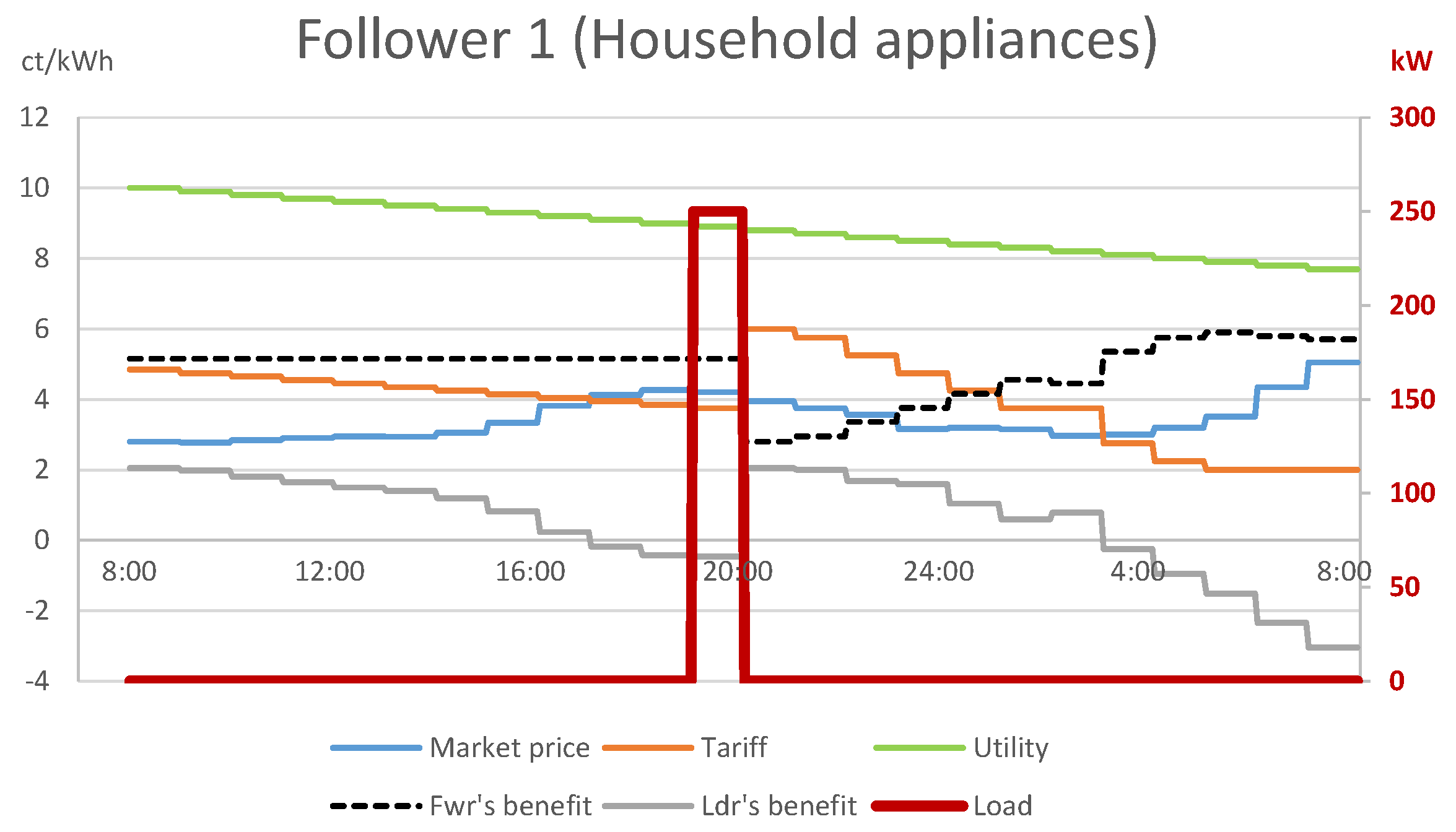
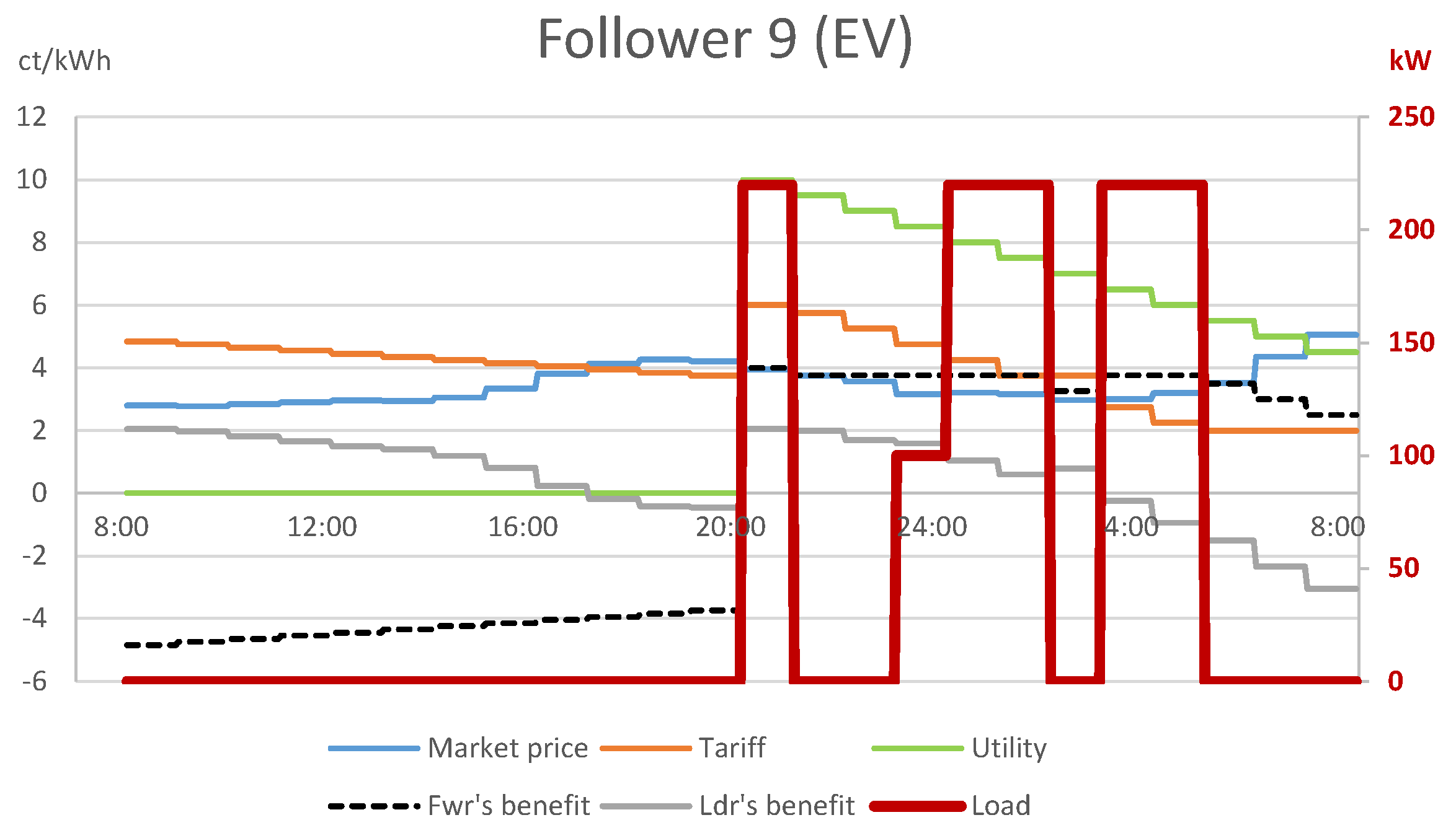
7.1. Numerical Example

This section demonstrates the proposed approach, and emphasizes the importance of being very conscious of the assumptions made, potentially implicitly, in regard to the way the followers select their response to the decision of the leader (e.g., the optimistic or the pessimistic assumption). In the example, the problem faced by an electricity retailer (leader) and its residential consumers (followers) is investigated on a daily time horizon divided into 24 hourly time units. Two types of consumers are distinguished, with household appliances and EV charging modeled as deferrable loads, respectively. Loads considered for the first consumer type were a 1.5 kW dishwasher and a 0.5 kW washing machine, both with a one-hour washing cycle. The consumers had slight preference for scheduling their load as early as possible, modeled with monotonously decreasing utility values. One-thousand such individual consumers were considered, organized into eight groups with different time windows for these loads. Each homogeneous consumer group was modeled as a separate follower, resulting in eight followers, each with $D_i^l=D_i^u=$ 250 kWh, $i=1,\dots ,8$.

The other type of consumers wished to charge their EVs, equipped with a 75 kWh battery from 20% to 100% using a 11 kW wall charger (which corresponds to the battery capacity of the most popular EV worldwide in 2019 and the power output of the corresponding charger). The EV was connected to the grid from 20:00 to 06:00 the next morning. These consumers had a stronger preference for scheduling their load as early as possible, in order to have their vehicles fully charged, even if they had to leave home earlier than usual. The ensemble of 20 such consumers is the 9th follower in the problem, with $D_9^l=D_9^u=$ 1200 kWh. For the sake of simplicity, other, inflexible loads are disregarded.

Market prices reflect the hourly prices recorded on the Hungarian power exchange (HUPX) on 1 January 2020, from 08:00, varying between 2.771 and 5.047 ct/kWh. The retailer must set an electricity tariff subject to $q_t^l=2$ ct/kWh and $q_t^u=6$ ct/kWh, for all t, with $Q=4$ ct/kWh.

Figure 1 displays the solution of this problem subject to the commonly applied optimistic assumption. The diagram shows the wholesale market price, the calculated tariff offered to consumers, the leader’s net benefit $(q_t-c_t)$ (ct/kWh, left vertical axis), and the grid-level load resulting from the followers’ demand response (kW, right vertical axis). With the appropriate tariff, the electricity retailer could motivate its consumers to schedule all their deferrable loads into periods when electricity is cheap, yet the retailer can realize a massively positive profit of 4983 cents.

A closer look into the sub-problem faced by follower 1 with household appliances (Figure 2) explains that the retailer achieved the above by compensating for the decreasing utility of followers 1–8 with a similar, decreasing tariff between 08:00 and 20:00, which resulted in a constant net benefit $(u_{i,t}-q_t)$ of 5.155 ct/kWh for followers 1–8 in this time interval. Since the followers were indifferent about the choice between these time periods, by the optimistic assumption, they decided on the period which was the most favorable for the leader: the period 08:00–09:00 in case of follower 1. In a similar fashion, the net benefit of follower 9 with EV charging (see Figure 3) was a constant 3.755 ct/kWh for 21:00–02:00 and 03:00–05:00. Hence, consumers charged their EVs in the period 21:00–02:00, to the benefit of the leader. However, this choice comes purely from an unnatural assumption of the mathematical model, which cannot be enforced in reality.

Given that various time periods bring similar net benefits for the followers, they may equivalently schedule their loads in other periods. Figure 4 depicts a solution in which the leader applies the same tariff, calculated using the optimistic assumption, but among periods that bring identical net benefits for the followers, they select the one that is the least favorable for the leader. In this case, followers 1–8 with household appliances schedule all their deferrable load into period 19:00–20:00 (see Figure 5), where the wholesale market price is higher than the tariff announced by the leader. Similarly, follower 9 charges the EVs partly in periods 03:00–05:00, resulting in further loss for the leader (see Figure 6). Hence, given that the retailer cannot realize its optimistic assumption, its assumed that positive profit can easily turn into considerable loss, −220 cents for the solution depicted.

At the same time, by Proposition 6, the leader can slightly modify the tariff to ensure that the followers have a unique optimal response, with loads identical to the optimistic solution and a tariff arbitrarily close to the optimistic tariff. Consequently, the profit of the leader is also arbitrarily close the the value calculated using the optimistic assumption. This pessimistic solution is not depicted in separate diagrams, since it is arbitrarily close to the optimistic solution displayed in Figure 1, Figure 2 and Figure 3.

7.2. Computational Experiments

Computational experiments investigated the efficiency and the scalability of the proposed approach on randomly generated problem instances of various sizes. Namely, the number of consumers (consumer groups), m, was taken from $\{5,10,15,20,25\}$, and the number of time periods, T, from $\{12,24,36,48\}$. Ten random instances were generated for each combination of m and T, resulting in 200 instances altogether.

The instances were similar in their structure to the numerical example presented above: half of the consumers captured different groups of households with deferrable loads (e.g., washing machines) that can be scheduled into a single time period. Other consumers modeled EV charging, where the load had to be distributed over 4–8 periods due to the upper bound $x_{it}^u$. In both cases, the load amounts, the time windows, and the utility values were generated randomly.

The proposed approach was implemented in FICO Xpress 8.8 in the Mosel programming language. During the experiments, the computational time required for solving the proposed MILP formulation (10) of the optimistic variant of the bilevel tariff optimization problem was measured. Given this optimistic solution, the pessimistic solution can be derived in negligible time using the pessimistic solution algorithm. The time limit was set to 300 s. All experiments were run on a personal computer with Intel i7-10510U 1.80 GHz CPU and 16 GB RAM.

The computational results are displayed in

Table 3. Results of computational experiments.

m	T	Opt	Time [s]	Gap [%]
				Avg.	Max.
5	12	10	0.08	-	-
	24	10	0.16	-	-
	36	10	0.72	-	-
	48	10	1.40	-	-
10	12	10	0.28	-	-
	24	10	2.73	-	-
	36	10	5.06	-	-
	48	10	13.92	-	-
15	12	10	1.83	-	-
	24	10	6.01	-	-
	36	10	30.85	-	-
	48	10	47.88	-	-
20	12	10	4.39	-	-
	24	8	81.29	0.58	5.34
	36	9	66.10	0.20	2.03
	48	7	172.74	1.37	12.76
25	12	10	5.00	-	-
	24	5	185.13	0.90	3.41
	36	5	250.15	2.12	11.81
	48	5	203.51	13.11	100.00

, where each row contains aggregated results over the 10 instances for a given problem size. Column Opt shows the number of instances solved to optimality out of 10; Time contains the average computation time in seconds; columns Gap/avg. and Gap/max. display the average and the maximum optimality gap for the given problem size. For each instance, the gap is computed as $(UB-LB)/UB$, where $UB$ and $LB$ are the upper and lower bounds, respectively.

The results show that the proposed approach could solve all instances with moderate sizes, i.e., with $m\le 15$ or $T=12$ to optimality in less than a minute. An increase of m has a stronger influence on the computational time than an increase of T. For larger problems, the solver often hit the time limit (for 10–30% of instances with $m=20$, and 50% of instances with $m=25$). In such cases, the optimality gap was reasonable, below 15% for all instances, except for a single instance with $m=25$ and $T=48$ for which the solver could not find an integer solution within the time limit; this is accounted for as a gap of 100%. For even larger instances, the development of more efficient solution algorithms is recommended.

8. Conclusions and Managerial Implications

This paper gave a detailed analysis of a simple bilevel tariff optimization problem for demand response management. Key properties of the optimal solutions were proven formally. It was shown that in some special cases with a single follower (e.g., when the electricity retailer can offer a dedicated tariff for an individual consumer) the optimal solution can be calculated analytically. For the general case with multiple followers, efficient solution approaches were proposed both for the optimistic and the pessimistic variants, based on a MILP formulation that exploited complementarity for the follower’s LP sub-problem. Hence, to the best of the authors’ knowledge, this paper proposed the first efficient exact solution approach for the pessimistic variant of the problem. Moreover, it was shown that in most cases, the supremum of the pessimistic variant equals the optimum of the optimistic variant, which means that with fully rational followers, the leader can attain a similar profit without the impracticable optimistic assumption.

8.1. Managerial Implications

The main finding of the research is related to the importance of defining clearly the assumption of how the followers select their response to the decision of the leader: almost all previous studies in the literature implicitly make the optimistic assumption that followers select the most favorable response for the leader, but this assumption cannot be enforced in practice. Instead, the followers typically have many optimal responses, and they may easily select another response that dramatically decrease the profit of the leader. This problem is addressed by the pessimistic variant of the bilevel problem, which assumes that the followers may select their optimal response that is the least favorable for the leader, and hence safeguards the leader from the consequences of an unexpected response. While the pessimistic variant of bilevel optimization problems is often harder to solve than the optimistic variant, this paper showed that for the studied bilevel tariff optimization problem, the pessimistic variant can also be solved efficiently.

8.2. Directions for Future Research

Future research should focus on generalizing the proposed approach to the pessimistic variant of richer bilevel models for energy management, including batteries and generators controlled by the leader or the followers, or specialized applications such, as HVAC. Moreover, the applicability of robust optimization approaches to these bilevel problems should be investigated, for instance, with uncertain consumer parameters or sub-optimal responses from followers.

References

1. de Souza Dutra, M.D.; Alguacil, N. Optimal residential users coordination via demand response: An exact distributed framework. Appl. Energy 2020, 279, 115851. [Google Scholar] [CrossRef]
2. Kovács, A. Bilevel programming approach to demand response management with day-ahead tariff. J. Mod. Power Syst. Clean Energy 2019, 7, 1632–1643. [Google Scholar] [CrossRef] [Green Version]
3. Wei, W.; Liu, F.; Mei, S. Energy Pricing and Dispatch for Smart Grid Retailers Under Demand Response and Market Price Uncertainty. IEEE Trans. Smart Grid 2015, 6, 1364–1374. [Google Scholar] [CrossRef]
4. Yu, M.; Hong, S.H. Supply-demand balancing for power management in smart grid: A Stackelberg game approach. Appl. Energy 2016, 164, 702–710. [Google Scholar] [CrossRef]
5. Zugno, M.; Morales, J.M.; Pinson, P.; Madsen, H. A bilevel model for electricity retailers’ participation in a demand response market environment. Energy Econ. 2013, 36, 182–197. [Google Scholar] [CrossRef]
6. Dempe, S. Foundations of Bilevel Programming; Kluwer Academic Publishers: Dordrecht, The Netherlands, 2002. [Google Scholar]
7. Cupelli, L.; Schumacher, M.; Monti, A.; Mueller, D.; De Tommasi, L.; Kouramas, K. Simulation Tools and Optimization Algorithms for Efficient Energy Management in Neighborhoods. In Energy Positive Neighborhoods and Smart Energy Districts; Monti, A., Pesch, D., Ellis, K., Mancarella, P., Eds.; Academic Press: Cambridge, MA, USA, 2017; pp. 57–100. [Google Scholar]
8. Bracken, J.; McGill, J.T. Mathematical programs with optimization problems in the constraints. Oper. Res. 1973, 21, 37–44. [Google Scholar] [CrossRef]
9. Bard, J.F. Practical Bilevel Optimization: Algorithms and Applications; Kluwer Academic Publishers: Dordrecht, The Netherlands; Boston, MA, USA, 1998. [Google Scholar]
10. Colson, B.; Marcotte, P.; Savard, G. An overview of bilevel optimization. Ann. Oper. Res. 2007, 153, 235–256. [Google Scholar] [CrossRef]
11. Boyd, S.; Vandenberghe, L. Convex Optimization; Cambridge University Press: Cambridge, UK, 2004. [Google Scholar]
12. Bard, J.F.; Falk, J.E. An explicit solution to the multi-level programming problem. Comput. Oper. Res. 1982, 9, 77–100. [Google Scholar] [CrossRef]
13. Ye, J.; Zhu, D. Optimality conditions for bilevel programming problems. Optimization 1995, 33, 9–27. [Google Scholar] [CrossRef] [Green Version]
14. Ye, J.J.; Zhu, D. New necessary optimality conditions for bilevel programs by combining the MPEC and value function approaches. SIAM J. Optim. 2010, 20, 1885–1905. [Google Scholar] [CrossRef]
15. Dempe, S.; Mordukhovich, B.S.; Zemkoho, A.B. Necessary optimality conditions in pessimistic bilevel programming. Optimization 2014, 63, 505–533. [Google Scholar] [CrossRef]
16. Dempe, S.; Mordukhovich, B.S.; Zemkoho, A.B. Two-level value function approach to non-smooth optimistic and pessimistic bilevel programs. Optimization 2019, 68, 433–455. [Google Scholar] [CrossRef] [Green Version]
17. Zeng, B. A Practical Scheme to Compute the Pessimistic Bilevel Optimization Problem. INFORMS J. Comput. 2020, 32, 1128–1142. [Google Scholar] [CrossRef]
18. Dempe, S.; Kalashnikov, V.; Pérez-Valdés, G.A.; Kalashnykova, N. Bilevel Programming Problems: Theory, Algorithms and Applications to Energy Networks; Springer: Berlin/Heidelberg, Germany, 2015. [Google Scholar]
19. Ben-Ayed, O. Bilevel linear programming. Comput. Oper. Res. 1993, 20, 485–501. [Google Scholar] [CrossRef]
20. Lozano, L.; Smith, J.C. A value-function-based exact approach for the bilevel mixed-integer programming problem. Oper. Res. 2017, 65, 768–786. [Google Scholar] [CrossRef]
21. Brotcorne, L.; Labbé, M.; Marcotte, P.; Savard, G. A bilevel model and solution algorithm for a freight tariff-setting problem. Transp. Sci. 2000, 34, 289–302. [Google Scholar] [CrossRef] [Green Version]
22. Loridan, P.; Morgan, J. Weak via strong Stackelberg problem: New results. J. Glob. Optim. 1996, 8, 263–287. [Google Scholar] [CrossRef]
23. Wiesemann, W.; Tsoukalas, A.; Kleniati, P.M.; Rustem, B. Pessimistic bilevel optimization. SIAM J. Optim. 2013, 23, 353–380. [Google Scholar] [CrossRef]
24. Kovács, A. On the Computational Complexity of Tariff Optimization for Demand Response Management. IEEE Trans. Power Syst. 2018, 33, 3204–3206. [Google Scholar] [CrossRef] [Green Version]
25. Wei, F.; Jing, Z.; Wu, P.Z.; Wu, Q. A Stackelberg game approach for multiple energies trading in integrated energy systems. Appl. Energy 2017, 200, 315–329. [Google Scholar] [CrossRef]
26. Yoon, A.Y.; Kang, H.K.; Moon, S.I. Optimal Price Based Demand Response of HVAC Systems in Commercial Buildings Considering Peak Load Reduction. Energies 2020, 13, 862. [Google Scholar] [CrossRef] [Green Version]
27. Jalali, M.; Zare, K.; Seyedi, H. Strategic decision-making of distribution network operator with multi-microgrids considering demand response program. Energy 2017, 141, 1059–1071. [Google Scholar] [CrossRef]
28. Nguyen, D.T.; Nguyen, H.T.; Le, L.B. Dynamic Pricing Design for Demand Response Integration in Power Distribution Networks. IEEE Trans. Power Syst. 2016, 31, 3457–3472. [Google Scholar] [CrossRef]
29. Soliman, H.; Leon-Garcia, A. Game-Theoretic Demand-Side Management With Storage Devices for the Future Smart Grid. IEEE Trans. Smart Grid 2014, 5, 1475–1485. [Google Scholar] [CrossRef]
30. Song, X.; Lin, H.; De, G.; Li, H.; Fu, X.; Tan, Z. An Energy Optimal Dispatching Model of an Integrated Energy System Based on Uncertain Bilevel Programming. Energies 2020, 13, 477. [Google Scholar] [CrossRef] [Green Version]
31. Vardanyan, Y.; Madsen, H. Stochastic Bilevel Program for Optimal Coordinated Energy Trading of an EV Aggregator. Energies 2019, 12, 3813. [Google Scholar] [CrossRef] [Green Version]
32. Zhang, Q.; Zhang, S.; Wang, X.; Li, X.; Wu, L. Conditional-Robust-Profit-Based Optimization Model for Electricity Retailers with Shiftable Demand. Energies 2020, 13, 1308. [Google Scholar] [CrossRef] [Green Version]
33. Alves, M.J.; Antunes, C.H. A semivectorial bilevel programming approach to optimize electricity dynamic time-of-use retail pricing. Comput. Oper. Res. 2018, 92, 130–144. [Google Scholar] [CrossRef]
Figure 1. Optimistic bilevel solution: grid-level consumption.
Energies 14 02095 g001
Figure 2. Optimistic bilevel solution: consumption of follower 1 with household appliances.
Energies 14 02095 g002
Figure 3. Optimistic bilevel solution: consumption of follower 9 with EV charging.
Energies 14 02095 g003
Figure 4. Optimistic tariff with the least favorable follower response: grid-level consumption.
Energies 14 02095 g004
Figure 5. Optimistic tariff with least favorable follower response: consumption of follower 1 with household appliances.
Energies 14 02095 g005
Figure 6. Optimistic tariff with the least favorable follower response: consumption of follower 9 with EV charging.
Energies 14 02095 g006