Large Eddy Simulation of Film Cooling with Forward Expansion Hole: Comparative Study with LES and RANS Simulations

Abstract

The forward expansion hole improves the film cooling effectiveness by reducing the penetration of the coolant jet into the main flow compared to the cylindrical holes. In addition, compound angles improve the film cooling effectiveness by promoting the lateral spreading of the coolant on a wall. Evidently, the combination of a compound angle and shaped hole further improves the adiabatic film cooling effectiveness. The film cooling flow with a shaped hole with 15° forward expansion, a 35° inclination angle, and 0° and 30° compound angles at 0.5 and 1.0 blowing ratios was numerically simulated with Large Eddy Simulations (LES) and Reynolds-averaged Navier–Stokes (RANS) simulations. The results of the time-averaged film cooling effectiveness, temperature, velocity, and root-mean-square (rms) values of the fluctuating velocity and temperature profiles were compared with the experimental data by Lee et al. (2002) to verify how the LES improves the results compared to those of the RANS. For the forward expansion hole, the velocity and temperature fluctuations in the LES contours are smaller than those of the cylindrical hole; thus, the turbulence and mixing intensity of the forward expansion hole are weaker and lower than those of the cylindrical hole, respectively. This leads to the higher film cooling effectiveness of the forward expansion hole. By contrast, the RANS contours do not exhibit velocity or temperature fluctuations well. These results are discussed in detail in this paper.

1. Introduction

In an ideal Brayton cycle, the gas turbine efficiency could be increased by an increase in the turbine inlet temperature [1]. However, if the turbine blades are not sufficiently cooled, the increased heat load can reduce the service life of the gas turbine and damage the turbine blade [2]. The surface temperature on the turbine blades should remain below an acceptable limit, and the film cooling technique is usually applied. The cooling air bled from the compressor is spread through small holes, thereby creating a thin cooling air film on the surface, which protects the blade from the hot mainstream flow.

Film cooling in gas turbines can be effectively investigated at a reasonable cost with computational fluid dynamics (CFD). Strong turbulence is formed in film cooling flow fields; this turbulence must be fully modeled with Reynolds-averaged Navier–Stokes (RANS) simulations or partially modeled with large eddy simulations (LES). The latter predicts the mixing state of the hot main flow and coolant jet better than RANS simulations. This is because the turbulent fluctuations are ensemble-averaged in RANS simulations, while LES resolves large-scale eddies directly in the turbulent flow, which results in more accurate predictions of film cooling flow fields [3,4,5,6].

A cylindrical hole shape has been commonly selected for film cooling holes owing to its simple structure and easy manufacture. Walters and Leylek (1997) investigated the film cooling effect of a cylindrical hole on a flat plate with the standard k–ε model [7]. They found that the reattachment of the injectant at high blowing ratios was not well predicted. In addition, they reported that the numerical simulations overpredicted centerline film cooling effectiveness (η_c); the results showed less lateral spreading of the coolant on the wall. McGovern and Leylek (2000) compared the effects of holes with 45°, 60°, and 90° compound angles with those of an ordinary cylindrical hole with the standard k–ε turbulence model [8]. They stated that the compound angle improved the lateral spreading of the coolant and increased the cooling effectiveness of the laterally averaged film compared to that created via the inclined inline injection from a hole. However, they discovered that the heat transfer coefficient increased owing to the effects of the compound angle injection. Moreover, Tyagi, and Acharya (2003) conducted LES to study the film cooling effect of a cylindrical hole [9]. The film cooling process resulted in complex flow fields and coherent structures; the LES results showed better predictions of η than the RANS simulations. Rozati and Tafti (2007) studied the effects of freestream turbulence on film cooling with a cylindrical hole using a leading-edge model with LES [10]. The fully turbulent jet increased the mixing with the main flow, which decreased the adiabatic film cooling effectiveness. They also reported that the turbulent injectant did not greatly affect the heat transfer coefficients, which were significantly affected by the near-wall turbulence. Johnson et al. (2011) investigated the effects of the length-to-diameter ratio, momentum ratio, and grid resolution on the film cooling process with a cylindrical hole with the realizable k–ε turbulence model [11]. They stated that the injectant with high momentum and short L/D ratio decreased η via the generation of a jet lift-off. In addition, refining the grid in the region near the hole’s trailing edge was important for obtaining good numerical results at high momentum ratios.

However, several researchers have reported that cylindrical holes can be relatively vulnerable to the penetration of injectant into the main flow, which decreases η. A specifically shaped hole can promote film cooling and therefore provide better thermal protection than cylindrical holes. When Goldstein et al. (1974) presented the results of film cooling experiments with shaped holes for the first time, shaped holes could not be adopted in applications with gas turbine blades because of the difficult manufacture [12]. Because the manufacturing techniques have evolved, shaped holes have been adopted in applications with real gas turbines. Bell, Hamakawa, and Ligrani (2000) experimentally investigated the spanwise-averaged film cooling effectiveness and Stanton number ratios of laterally and forward-diffused holes [13]. In addition, they investigated the effects of a shaped hole with a 45° compound angle. The shaped holes increased the film cooling effectiveness because of less jet penetration, better diffusion of cooling air, lower velocity gradients at the exit, and increased lateral spreading of the cooling air. They found that a laterally diffused hole with a compound angle exhibits the best film cooling effect at blowing ratios from 0.7 to 1.8. Furthermore, Hyams and Leylek (2000) numerically studied the effects of forward-diffused, laterally diffused, inlet shaped, and cusp shaped holes on the film cooling effectiveness and flow fields [14]. The spreading of the coolant in the lateral direction from the forward-diffused hole was weak, although the cooling performance along the centerline was good. Because the laterally diffused hole provided the best film cooling performance, the researchers concluded that the shaped holes greatly affected the film cooling performance. Wang et al. (2018) investigated the interaction between the main flow and injectant in a fan-shaped hole whose cross-sectional shape at the hole exit looked like a fan with the blowing ratio, M = 0.5 and 1.0 with LES [15]. Numerous hairpin vortices were randomly distributed downstream of the hole. Moreover, the roller and horseshoe vortices were weaker than those in the cylindrical hole system. The researchers found plenty of small-scale vortices due to the break-up of large-scale coherent vortex structures in the far-field region of the hole. Oliver, Bogard, and Moser (2019) investigated the effect of the Mach number of the main flow on the film cooling performance of a 7-7-7 shaped hole representing a fan-shaped hole with forward, left, and right lateral expansion angles of 7 degrees with LES [16]. When the Mach number of the main flow was 0.5, the spanwise-averaged film cooling effectiveness decreased up to approximately 50% with respect to that at a Mach number of 0.25; the researchers concluded that the Mach number of the freestream could substantially affect η. They stated that the reason for the decrease in the effectiveness at high Mach numbers was the separation and large-scale oscillation of the coolant in the hole. Furthermore, Wang, Su, and Yuan (2020) studied the effect of the cross-flow on the film cooling process on an end wall and the flow fields of a 7-7-7 shaped hole with the LES Smagorinsky–Lilly model [17]. The cross-flow caused the counter-rotating vortex pair (CRVP) to be asymmetric. In addition, the large-scale vortices induced by the cross-flow greatly affected the shapes and convection of the vortices (e.g., hairpin and horseshoe vortices), thereby substantially affecting the distribution of the cooling air. Zamiri, You, and Chung (2020) optimized the geometry of the laidback fan-shaped hole to optimize the film cooling performance with LES [18]. They chose three parameters (the metering length, forward expansion angle, and lateral expansion angle) as the design variables; η of the optimized fan-shaped hole was increased by approximately 50% compared to that of an ordinary hole.

Although some LES predictions of the film cooling effect of shaped holes have been published, the phenomenon has not been thoroughly discussed. In the current study, the effects of the forward expansion hole system with compound angles of 0° and 30° on the film cooling performance at blowing ratios of M = 0.5 and 1.0 were investigated, and the LES results were compared with experimental data and RANS predictions. More specifically, time-averaged η, temperature contours, time-averaged velocity profiles, and contours of velocity and temperature fluctuations predicted with LES were compared with the RANS results. Because the LES simulations require excessively high computation time, most gas turbine manufacturers wonder if RANS simulations could be a good alternative for predicting the film cooling flow fields. The main goal of the presented study was to verify that the LES film cooling results of a forward expansion hole are better than the RANS results.

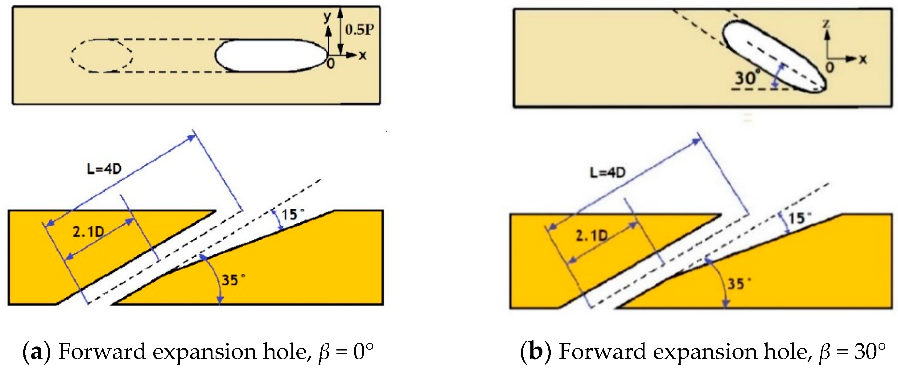
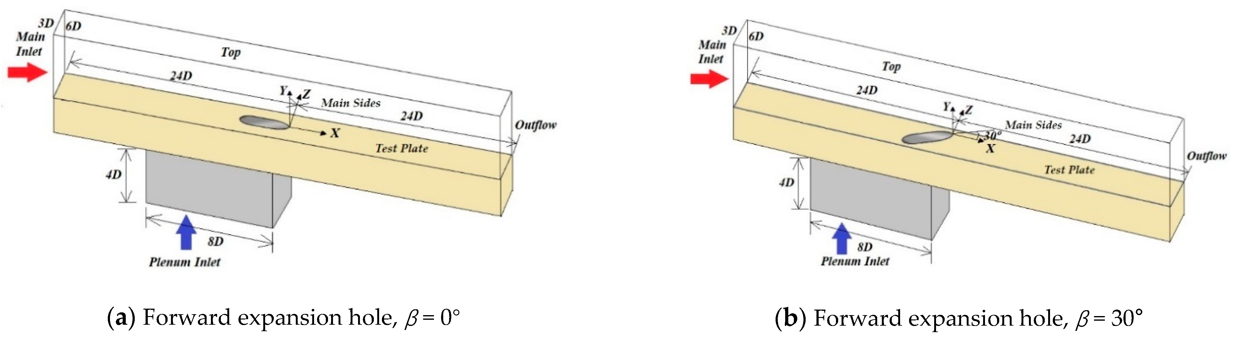
2. Geometry and Boundary Conditions

Figure 1 presents schematics of the forward expansion hole configurations with compound angles β of 0° and 30°; Figure 2 illustrates the computational domains of the forward expansion holes. The geometry of the forward expansion hole system was based on those presented in [19] in which the experimental equipment had a row of seven cooling holes. The compound angle β is the angle between the streamwise direction and projected injection vector on the x–z plane. The single-shaped hole configuration was adopted, and periodic boundary conditions were applied at the spanwise centerline between the holes (z = ±1.5 D) to reduce the computational cost. The diameter of the lower hole (D), the ratio of the hole length to the hole diameter, L/D, the angle of injection (α), and the ratio of the pitch between holes to the hole diameter, P/D were 15 mm, 4, 35°, and 3, respectively.

Table 1. Boundary conditions of the domain.

Surface	Boundary Condition
Main inlet	Velocity inlet (u = constant)
Plenum inlet	Velocity inlet (u = constant)
Top	Symmetry ($\frac{\partial \mathrm{u}}{\partial \mathrm{y}}=0,\frac{\partial \mathrm{w}}{\partial \mathrm{y}}=0,\mathrm{v}=0$)
Test plate	Adiabatic wall (u = v = w = 0)
Outflow	Pressure outlet
Main sides	Periodic (u(x, y, z, t) = u(x, y, z + P, t), ΔP = 0)
Sides of plenum	Wall (u = v = w = 0)
Hole wall	Wall (u = v = w = 0)

shows the boundary conditions of the domain. The turbulence intensity of the main flow was 0.2% at the main inlet, and the main flow velocity was 10 m/s. The vortex method as the fluctuating velocity algorithm was adopted at the main inlet, and 190 vortices were injected in the inlet plane to generate turbulent inflow conditions. At the inlets, the temperature of the main flow was 313 K, and the coolant temperature was 293 K.

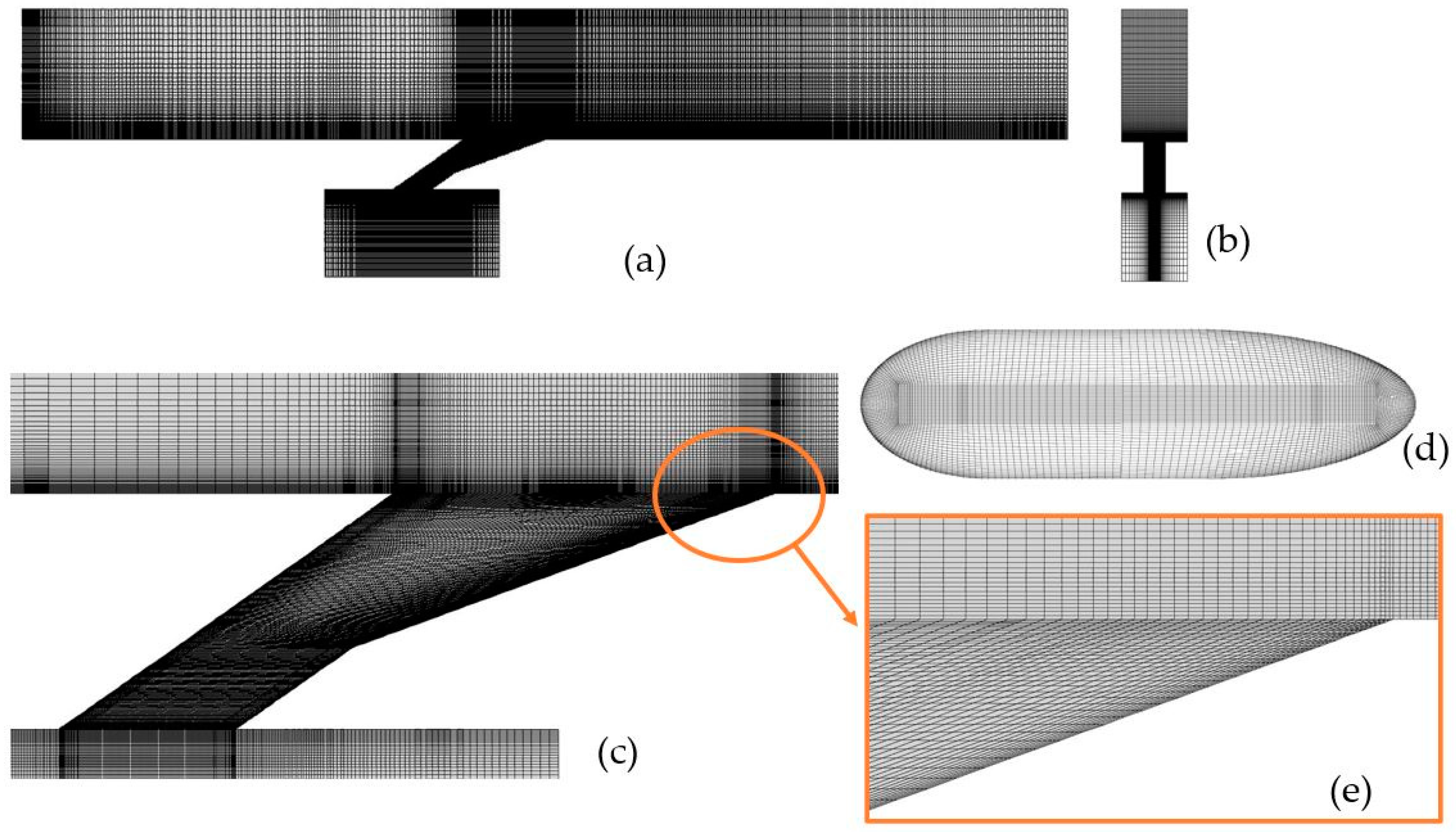
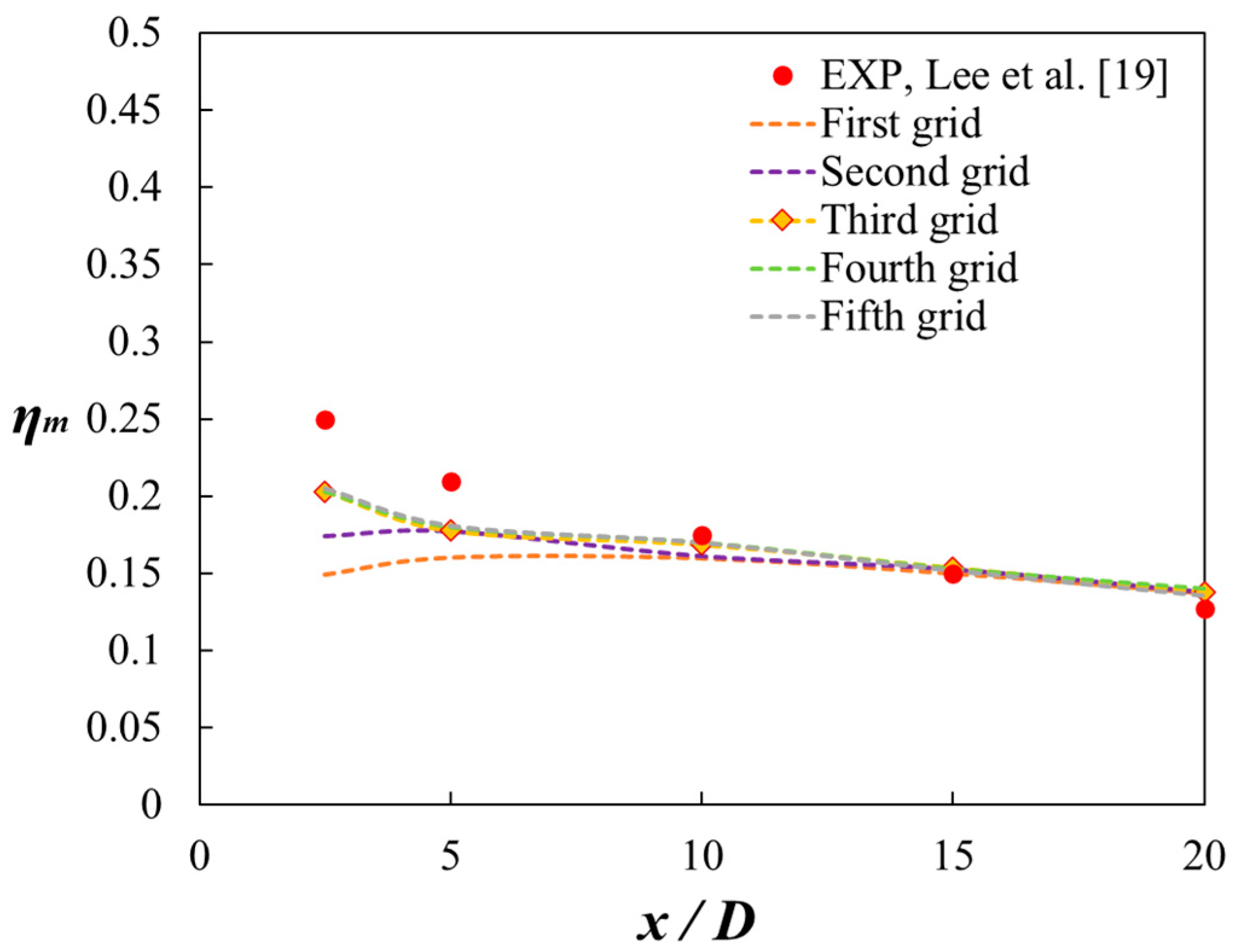
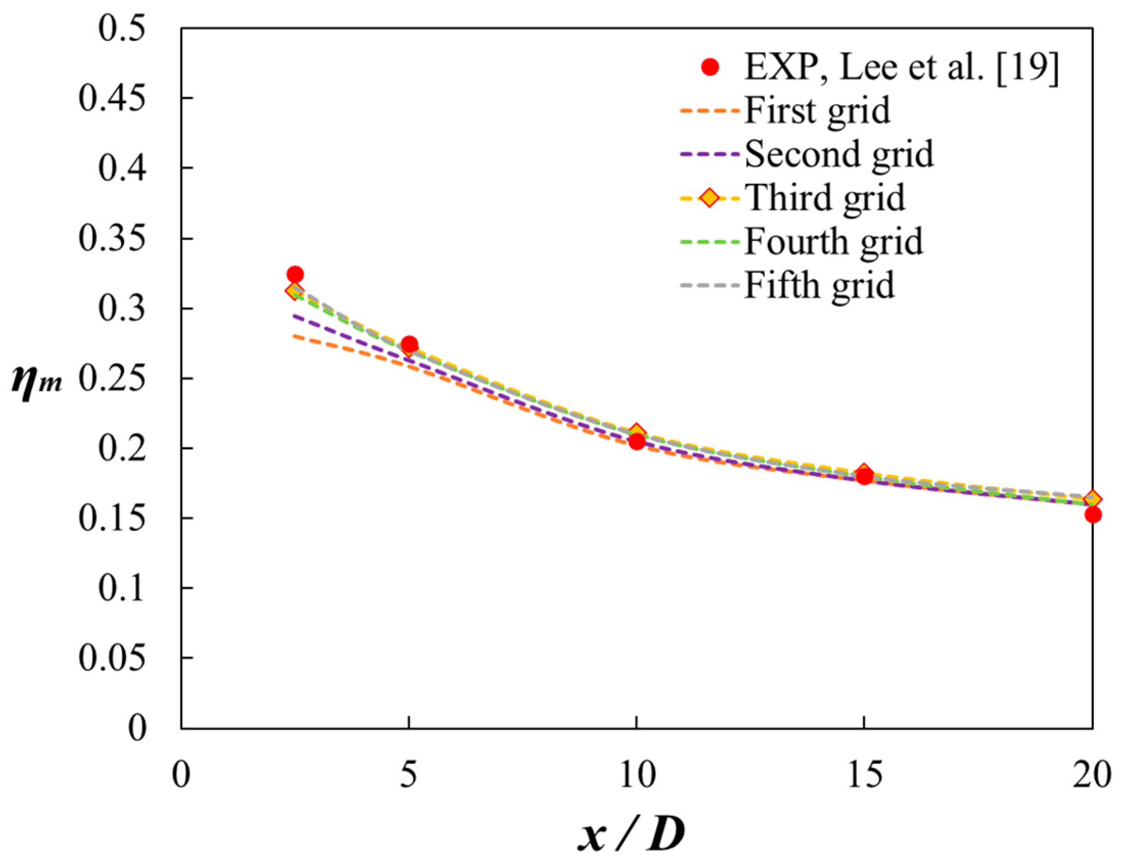
3. Validation of Numerical Methods

The numerical calculations were conducted by ANSYS Fluent v.19.1 (ANSYS, Canonsburg, PA, USA) [20], and the meshes were formed in Pointwise v.18.1 (Pointwise, Fort worth, TX, USA) [21]. The LES was executed with the Smagorinsky–Lilly model as the subgrid-scale model because it was shown that the Smagorinsky–Lilly model predicted the best results for the film cooling effectiveness compared to the results by other models in ANSYS Fluent such as kinetic energy transport model, WMLES (Wall-Modeled Large Eddy Simulation) and WALE (Wall-Adapting Local Eddy-Viscosity) [22]. The 6.25 × 10⁻⁶ s time step means that the mainstream convects the hole diameter after 400-time steps [23,24]. The maximum Courant–Friedrichs–Lewy (CFL) number was less than one (U∆t/∆x = 0.3125) [25]. After the solution had reached a statistical steady state, the statistics of the solution were collected for about 20 flow-through times for the main flow (about 0.5 s). The LES runtime with an Intel Xeon Gold 6148 processor 16 cores was approximately 6–7 weeks in each case. In addition, the fluid was assumed to be Newtonian and incompressible with temperature-dependent properties. The compressibility was negligible because the main flow velocity was 10 m/s (Mach number of 0.029), and the jet injection velocities were 5 and 10 m/s at blowing ratios of M = 0.5 and 1.0, respectively [26]. The governing equations are the incompressible Navier–Stokes and energy equations. Moreover, the Semi Implicit Method for Pressure Linked Equations (SIMPLE) scheme was used; the convection term was solved with the second-order upwind scheme, and the diffusion term was solved via central differencing. In the LES, the governing equations were transformed into a filtered equation [20,27,28]. The governing equations [29,30] were not shown here because a commercial CFD code was used. Figure 3 illustrates the meshes of the forward expansion hole system, including the mesh configuration in the x–y plane, the mesh configuration in the y–z plane, close-up of the mesh near the cooling hole, and mesh configuration at the hole exit. The LES and RANS simulations were conducted in the same mesh in the figure.

Figure 4 and Figure 5 show the grid sensitivity results of the spanwise-averaged effectiveness at x/D = 2.5 in the forward expansion hole with β = 0° and 30° at a blowing ratio of M = 0.5; the grid characteristics are presented in

Table 2. Specifications of the cell number for grid sensitivity test of forward expansion hole with β = 0°.

Grid	Number of Cells in x Direction	Number of Cells in y Direction	Number of Cells in z Direction	Number of Cells in Cross Flow Block (Million)	Total Cell Number (Million)
First	320	70	70	1.89	4.49
Second	502	75	76	3.18	5.78
Third	552	80	82	3.94	6.53
Fourth	602	85	86	4.72	7.31
Fifth	682	90	90	5.85	8.45

and

Table 3. Specifications of the cell number for grid sensitivity test of forward expansion hole with β = 30°.

Grid	Number of Cells in x Direction	Number of Cells in y Direction	Number of Cells in z Direction	Number of Cells in Cross Flow Block (Million)	Total Cell Number (Million)
First	426	70	92	3.06	5.65
Second	480	75	102	3.99	6.59
Third	530	80	114	5.16	7.75
Fourth	560	85	124	6.22	8.82
Fifth	594	88	134	7.32	9.91

.

The results were obtained with the LES Smagorinsky–Lilly model for five different meshes. As shown in Figure 4 and Figure 5 the effectiveness value along x/D = 2.5 on the third grid approximately matches those of the finer fourth and fifth grids. Thus, a 6.53 million-cell grid for β = 0° and a 7.75 million-cell grid for β = 30° were selected to model the film cooling effect in the system with the forward expansion hole.

4. Results and Discussion

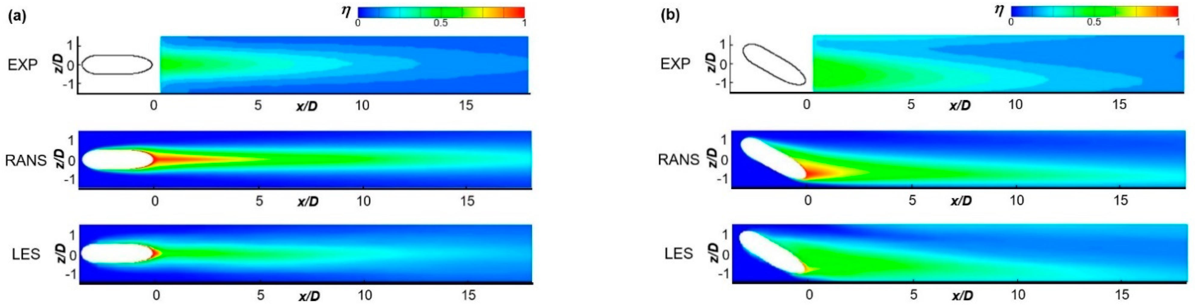
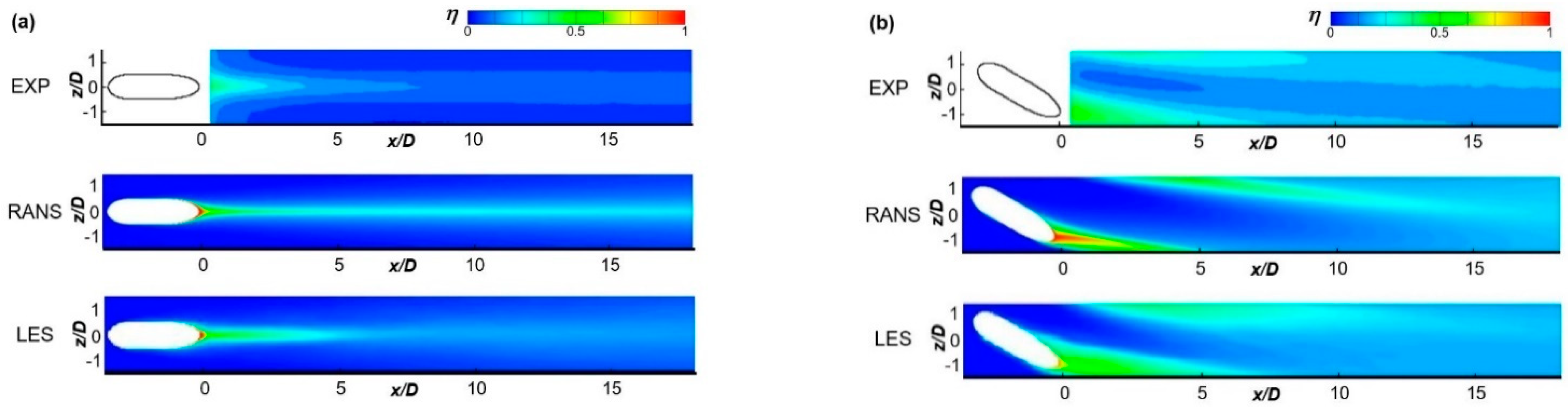
4.1. Contours of Time-Averaged η

Figure 6 and Figure 7 display the contours of the time-averaged film cooling effectiveness on the wall; these results were compared with the experimental data presented in [19,31]. As indicated by the contours of the experimental results, when a compound angle (β) of 30° is adopted, and the coolant is injected at a spanwise velocity, the coolant spreading in the lateral direction on the wall is more effective than that for a compound angle of 0° because the CRVP is asymmetric [32]. At a β of 30°, the effect of the CRVP decreased, and the entrainment of the hot cross-flow under the injectant is weakened, which leads to a more uniform coolant coverage and increased lateral-averaged η. As illustrated in the figures of the experimental data, the effect of the compound angle was more pronounced at a blowing ratio of 1.0 than at a blowing ratio of 0.5. The RANS and LES contours showed this trend well. However, the RANS simulations overpredicted the film cooling effectiveness in the narrow region near the cooling hole; by contrast, the LES results exhibited more similar contours to those of the experimental data, although the spreading of the coolant in the lateral direction in the LES results was less effective than in the experimental results.

Figure 8 and Figure 9 display the cross-sectional time-averaged dimensionless temperature contours of the forward expansion hole with β = 0° and 30° for blowing ratios of M = 0.5 and 1.0 at x/D = 2.5, 5, and 10, respectively. For the shaped hole with β = 30°, the cooling air was injected at a spanwise velocity. As the mainstream flow moves downstream and the x/D value increases, the dimensionless temperature of the coolant decreased because of the coolant dispersion caused by the mixing mainstream flow and injectant. The contours illustrate that the outlines of the dimensionless temperature contours of the LES and RANS results showed no significant differences. However, the dimensionless temperature of the coolant core area in the RANS results was higher than that in the LES results because the mixing intensity between the hot mainstream flow and injectant in the RANS results was not as high as in the LES results. Moreover, the outlines of the dimensionless temperature of the coolant in the RANS results were more circular than those in the LES results owing to less mixing. In addition, as shown in Figure 8f, for β = 30°, the contours of the coolant from the neighboring hole were more clearly visible in the LES contours than in the RANS contours because the cooling air spread more between adjacent holes on the test plate in the LES. This is also shown in Figure 6 and Figure 7.

At a blowing ratio of 1.0, the location of the coolant core was lifted up with respect to that at M = 0.5 because of the high momentum of the injectant; however, the jet lift-off in the forward expansion hole was not as large as that of the cylindrical hole because the injection velocity of the coolant is lower in the first scenario [33]. In Figure 10 and Figure 11, the mean streamlines are superimposed on the cross-sectional time-averaged contours of the dimensionless temperature at x/D = 2.5 and M = 0.5 and 1.0, respectively. Without a compound angle (β = 0°), symmetric CRVPs were generated in the LES and RANS contours. The CRVP (i.e. the kidney vortices) promoted the coolant lift-off, which resulted in stronger entrainment of the hot gas under the coolant.

At M = 1.0, the intensity of the CRVP is increased owing to the increased coolant mass flow, and entrainment of the hot air of the mainstream flow is stronger compared to that at M = 0.5. For a compound angle (β) of 30°, the CRVP transformed into a single vortex, as shown in the LES and RANS flow patterns. The streamlines in the LES and RANS results were similar, and the locations of the vortex centers are approximately identical; however, the outlines of the RANS contours are more circular than those of the LES contours due to the weaker mixing of the cooling air with the cross-flow.

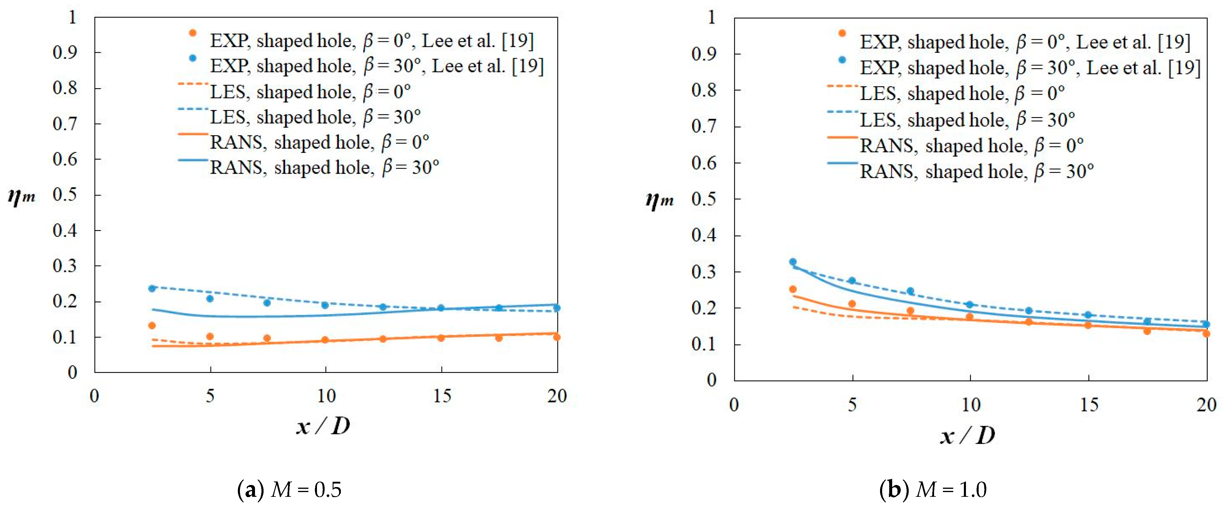
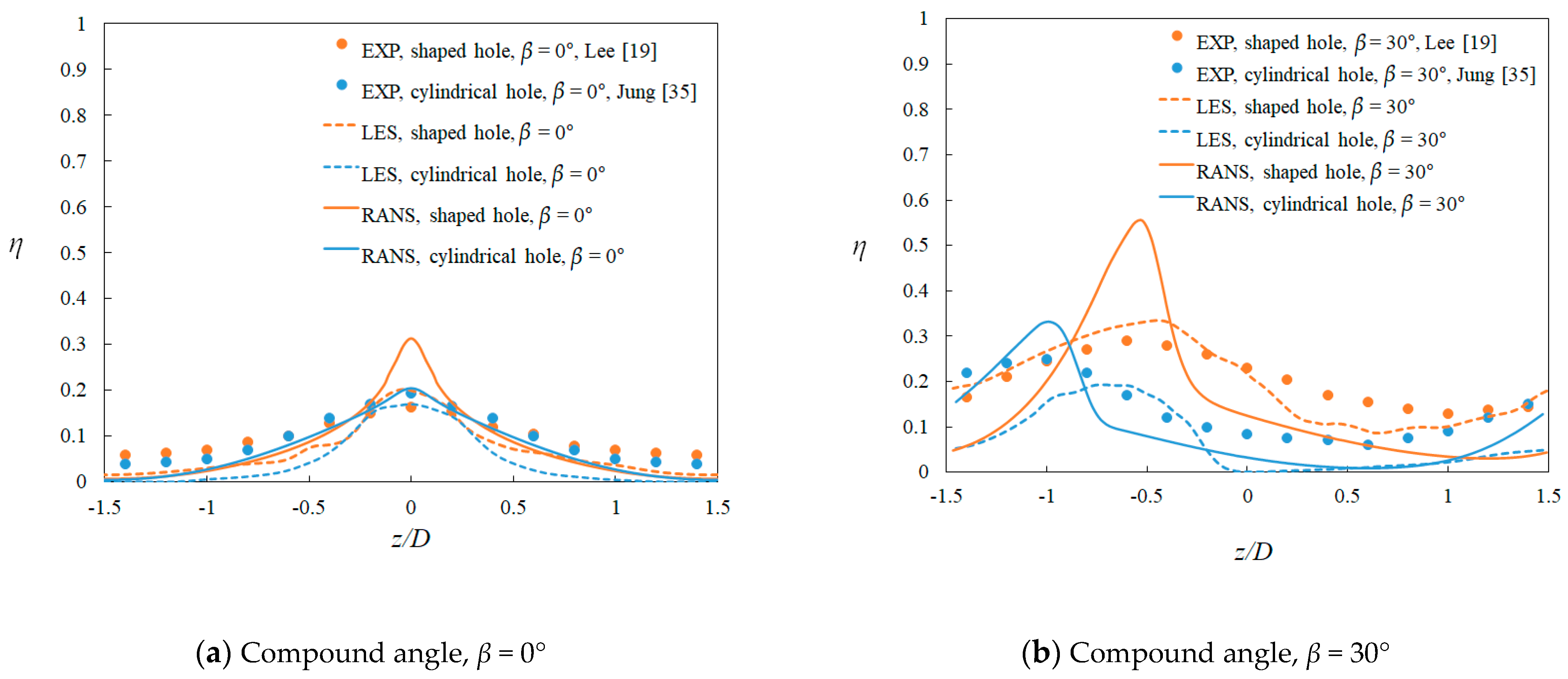
4.2. Time-Averaged Film Cooling Effectiveness

Figure 12 displays the spanwise-averaged film cooling effectiveness as a function of x/D at blowing ratios of 0.5 and 1.0. The spanwise-averaged film cooling effectiveness obtained with LES and RANS simulations agreed well with the experimental data, except for the narrow region near the cooling hole. In particular, for a compound angle of 30°, the LES predicted the film cooling effectiveness better than the RANS simulations. For β = 30°, the average difference in the spanwise-averaged effectiveness between the experimental data and LES results was approximately 3%, while the difference between the experimental data and RANS results was approximately 6%, and the deviations were mostly attributed to the difference in the effectiveness around the narrow region near the hole. Considering the deviations in LES results were similar to that in RANS results, RANS could be a good alternative for predicting the spanwise-averaged effectiveness of forward expansion holes because RANS over-predicted the centerline effectiveness for β = 0°, while it underpredicted core jet dissipation and lateral spreading of the coolant. Thus, the spanwise-averaged effectiveness became similar to the experimental data.

Figure 13 and Figure 14 illustrate the time-averaged spanwise film cooling effectiveness at x/D = 5 and blowing ratios of 0.5 and 1.0, respectively. Although the RANS results of the spanwise-averaged effectiveness agreed well with the experimental data in Figure 12, the local distributions of the film cooling effectiveness in the spanwise direction predicted with RANS simulations and experimental data did not agree well. The RANS simulations overpredicted the film cooling effectiveness, whereas the LES results show more accurate predictions for the local film cooling effectiveness.

For a shaped hole with β = 30°, the spanwise effectiveness obtained with the RANS simulations at x/D = 5 and M = 0.5 differed by approximately 77% from the experimental data, whereas the spanwise effectiveness obtained with the LES exhibited a 15% deviation from the experimental data. The different prediction results are attributed to the lower predicted mixing characteristics of the mainstream and coolant in the RANS simulations compared to those of the actual case. As previously mentioned, RANS simulations could be a good alternative for the prediction of the spanwise-averaged film cooling effectiveness because the respective results agreed well with the experimental data. However, considering that the thermal damage on turbine blades is usually generated by poor local cooling characteristics, it can be concluded that LES instead of RANS simulations should be used to predict the local film cooling effectiveness on turbine blades.

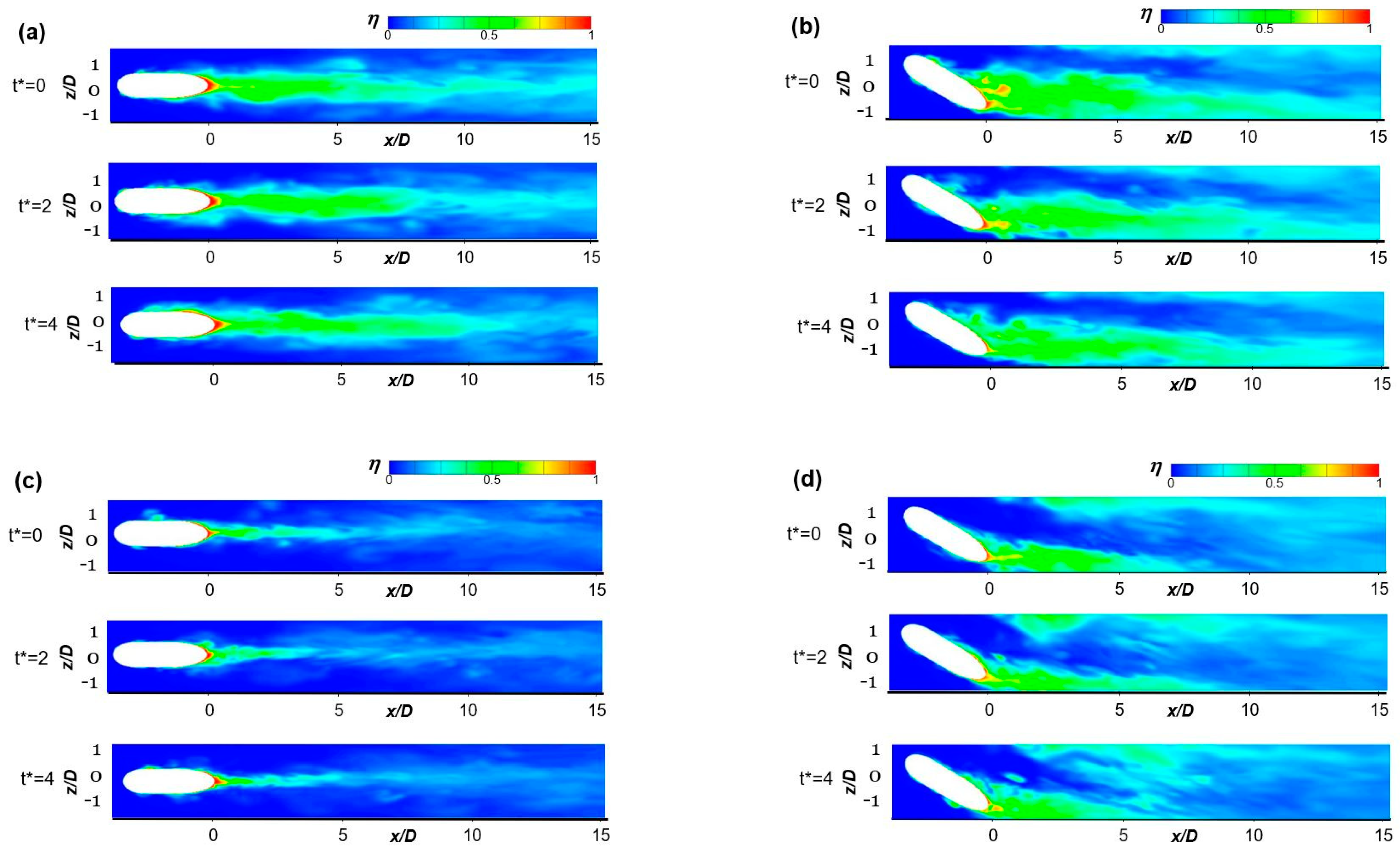
4.3. Contours of Instantaneous Film Cooling Effectiveness on Wall

Figure 15 shows the contours of the instantaneous film cooling effectiveness on the test plate obtained with LES at β = 0° and 30° and M = 0.5 and 1.0. The variable t* represents the dimensionless time defined by the main flow velocity and hole diameter; t* = 1 is the time required for the mainstream flow to travel across the hole diameter. The figure shows the LES contours of the instantaneous film cooling effectiveness under steady conditions at t* = 0, 2, and 4; the contours were not significantly different. For a compound angle of 30°, the contours exhibit a wider cooling air spread in the lateral direction than those for β = 0°, as shown by the mean contours in Figure 6 and Figure 7. Even in the forward expansion hole configuration, for β = 0°, the coverage area of the coolant on the wall at M = 1.0 was distinctly smaller than that at M = 0.5; however, the coverage area of the cooling air was wider for a compound angle of 30°.

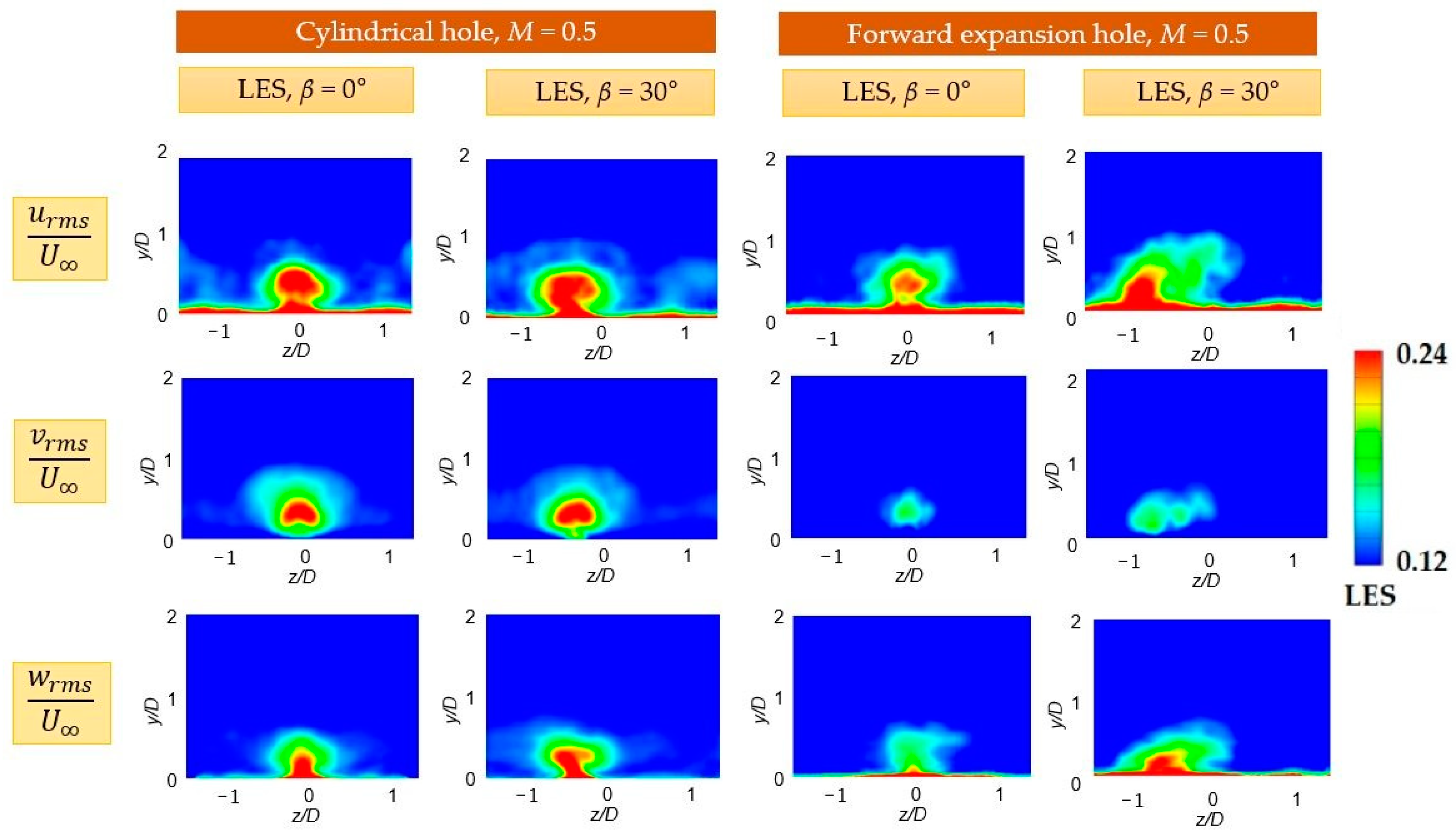
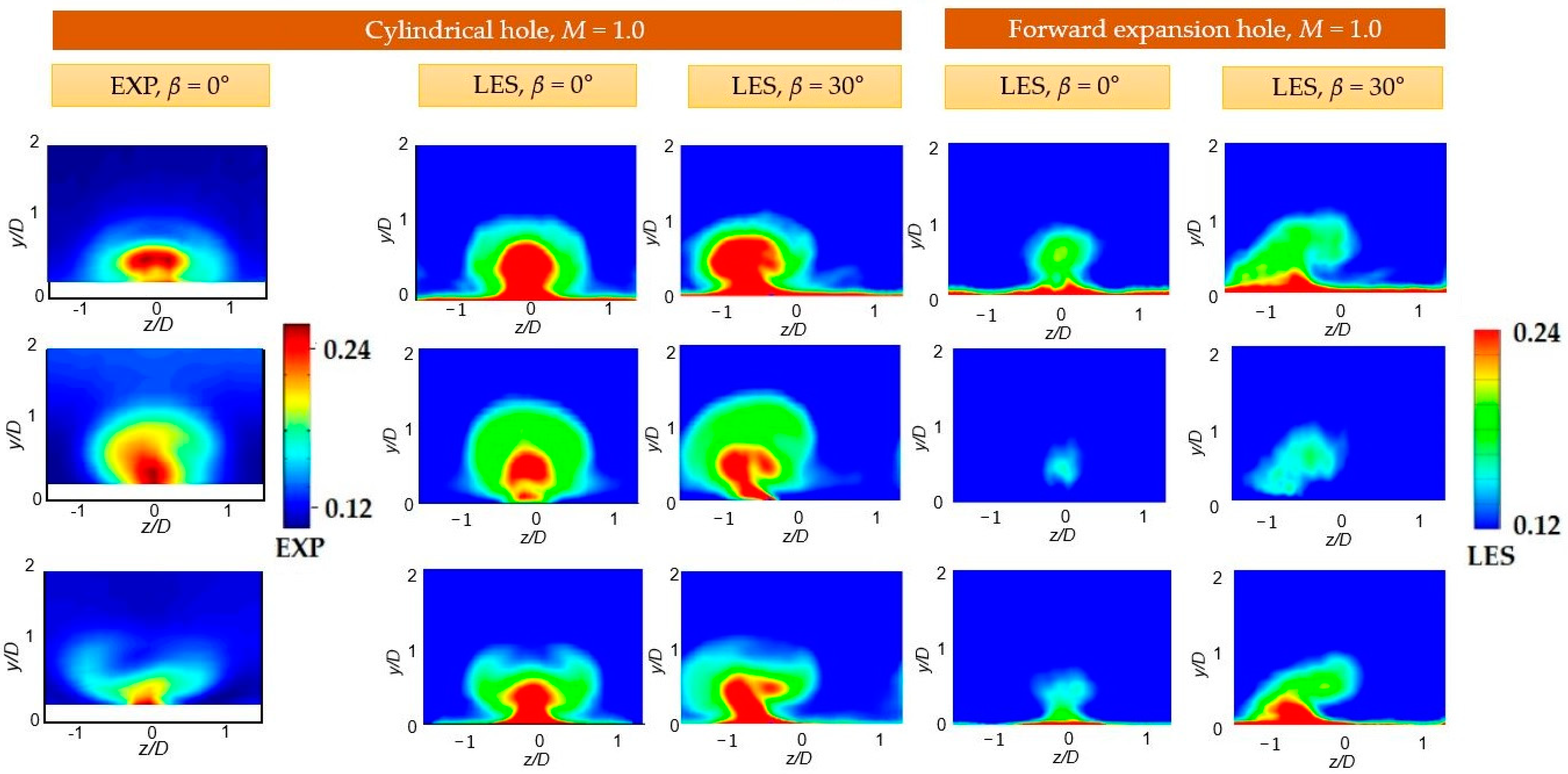
4.4. Contours of Velocity Fluctuation on Streamwise-Normal Plane

Figure 16 and Figure 17 present the turbulence intensity for the components u, v, w predicted in the LES for the blowing ratio of 0.5 and 1.0, respectively. For β = 0°, the contours for M = 1.0 were compared to those of the experimental data of Burd et al. [34]. The contours of the cylindrical hole in the figures originate from [33]. The outlines of the contours obtained by the experiment were similar to those obtained by LES even though the areas with the highest values of turbulence intensity in the x, y, and z directions were somewhat different. Compared with the contours of the time-averaged dimensionless temperature and streamlines in Figure 10 and Figure 11, the maximum values of the turbulence intensity were generated around the upward flow in the vortex, while the turbulence intensity around the downward flow in the vortex was very low. The results of the RANS model showed extremely small velocity fluctuations compared to those of the LES contour range, and only the velocity fluctuations obtained with the LES are shown in Figure 16 and Figure 17. The overall velocity fluctuations of the forward expansion hole were smaller than those of the cylindrical hole; thus, the turbulence intensity of the forward expansion hole is lower than that of the cylindrical hole, thereby leading to the better film cooling effectiveness of the former. In particular, the v_rms/U_∞ values of the forward expansion hole were greatly decreased compared to those of the cylindrical hole as the injection velocity in the normal direction was decreased by increased cross-sectional area at the forward expansion hole exit. When the compound angle was 30°, the contours of the velocity fluctuations showed that the distribution of the turbulence intensity had shifted along the −z-direction because the coolant was injected at a spanwise velocity, as shown in Figure 6 and Figure 7.

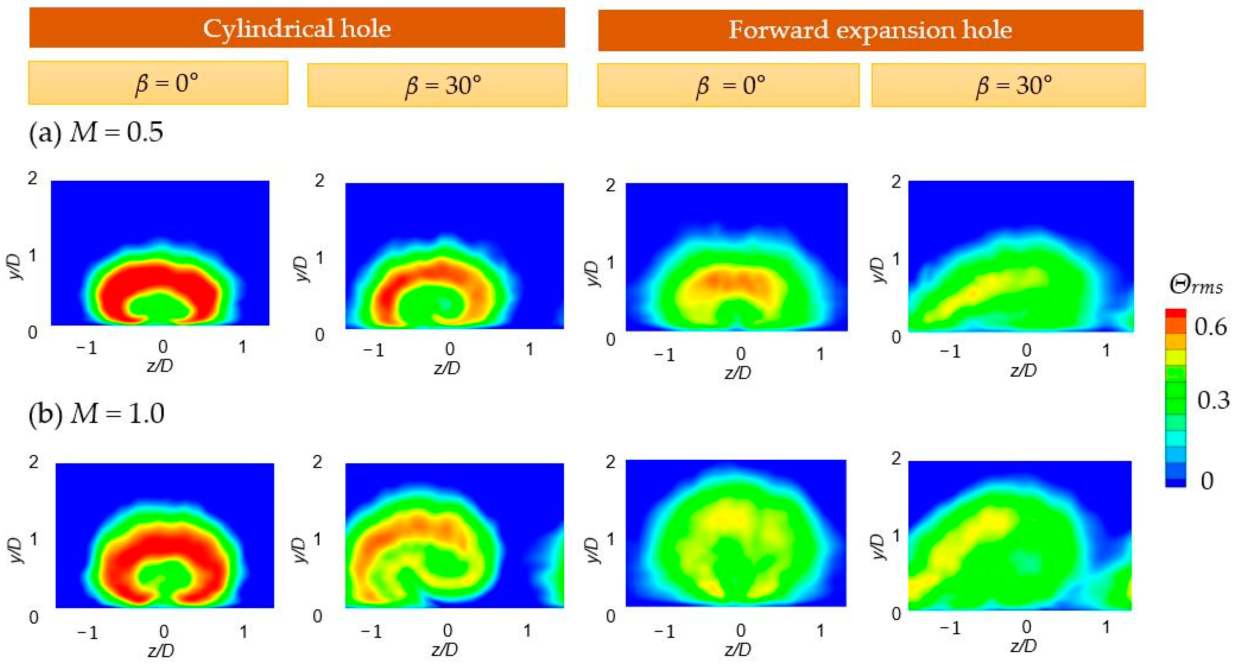
4.5. Contours of Temperature Fluctuations on Streamwise-Normal Plane

Figure 18 shows the time-averaged cross-sectional contours of θ_rms at x/D = 2.5. Like the contours of the velocity fluctuations in Section 4.4, the prediction results of the RANS model showed extremely small temperature fluctuations compared to those of the LES contour range, and only the temperature fluctuations obtained with the LES are shown in the figure. High θ_rms is connected to the large gradients in the mean temperature contour illustrated in Figure 8 and Figure 9, indicating that the mixing intensity between the hot mainstream flow and injectant around the area with high θ_rms is high and the area with high-temperature fluctuation was larger than the area with large velocity fluctuations in Figure 16 and Figure 17. As indicated by the contours, for the shaped hole with β = 0°, the maximum of θ_rms was higher than that for β = 30°; thus, the mixing intensity for β = 0° was higher than that for β = 30°, which resulted in a higher η on the test plate for β = 30°. The mixing of the hot main flow and coolant was supported by numerous vortices such as hairpin, horseshoe, and roller vortices; these vortices were weakened in the forward expansion hole with β = 30° compared to that in the case with β = 0°. In addition, the maximal θ_rms of the shaped hole was much lower relative to the contours of the cylindrical hole; this resulted in a higher film cooling performance in the shaped hole configuration compared to that in the cylindrical hole system.

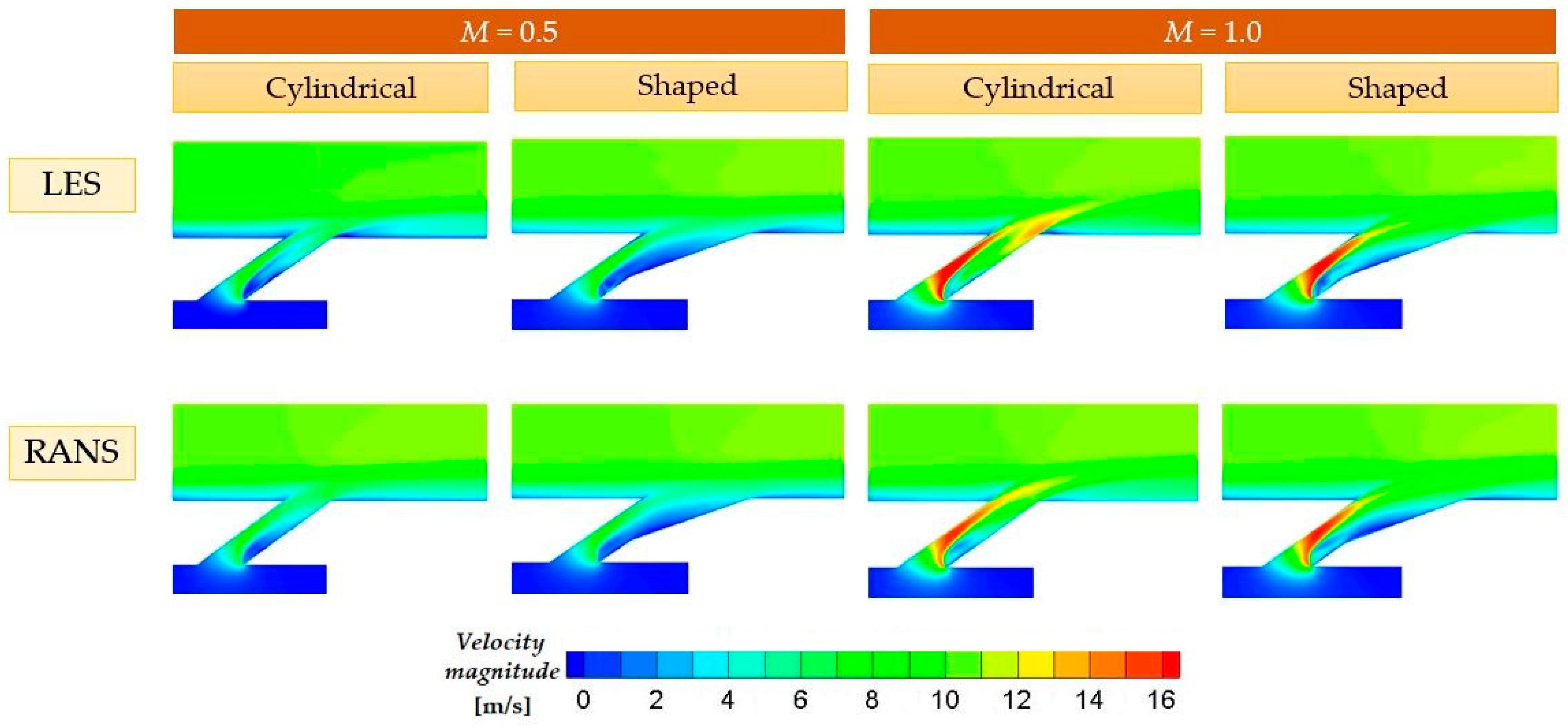
4.6. Time-Averaged Velocity Magnitude Contours in Hole

Figure 19 depicts the contours for the time-averaged velocity magnitude on the x–y plane obtained with LES and RANS simulations for blowing ratios of 0.5 and 1.0. The contours in the cylindrical hole were added as a baseline. Only the contours for the shaped hole with β = 0° are shown because the contours for β = 30° were almost identical. In the forward expansion hole, the mean velocity magnitude of the injectant around the trailing edge of the hole exit was lower than that in the cylindrical hole because of the expanded hole area around the exit. The regions with high velocities in the hole due to the separated coolant flow are evident in Figure 19. The contours obtained with RANS and LES simulations exhibit small differences in the mean velocities in the hole; however, in the LES contours, the time-averaged velocity magnitude of the injectant at the hole exit was slightly higher than that of the RANS contours; this led to the better penetration of the coolant into the hot main flow and the lower film cooling effectiveness.

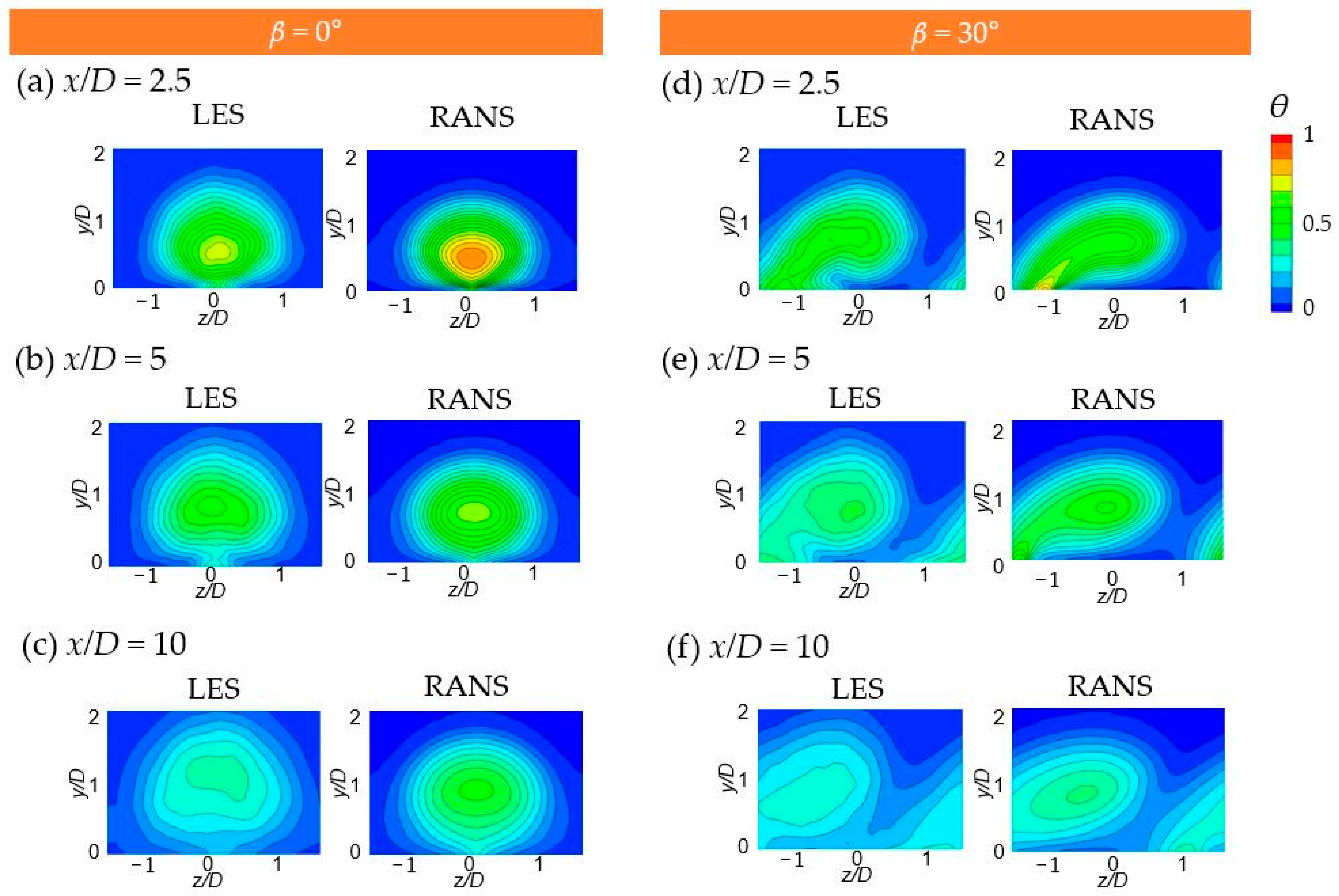
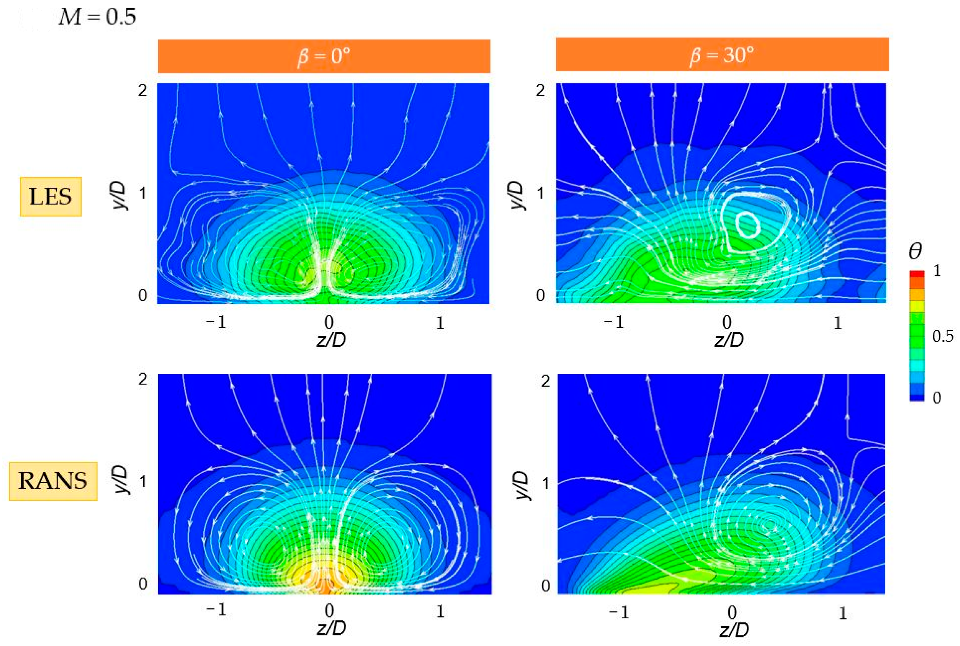
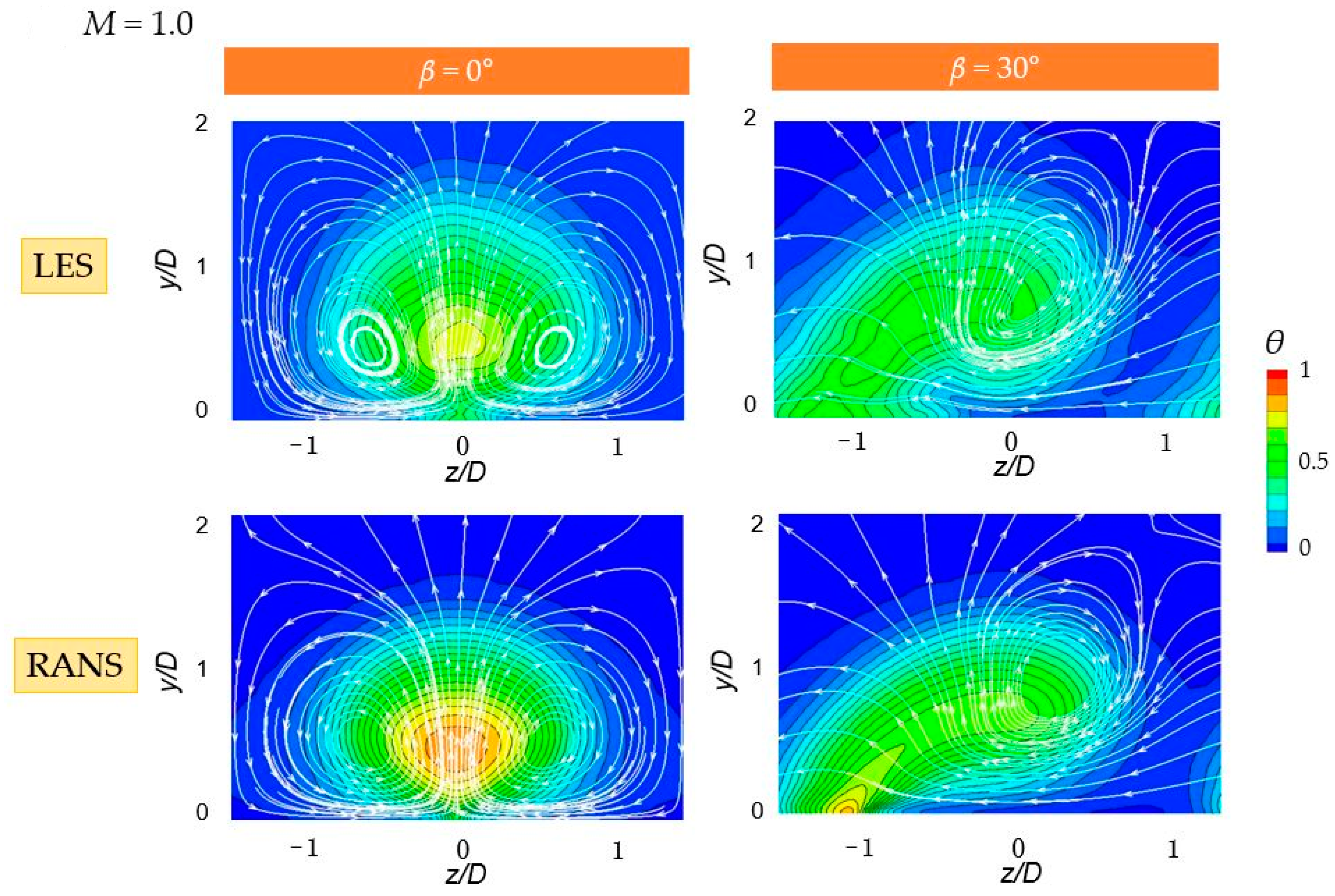
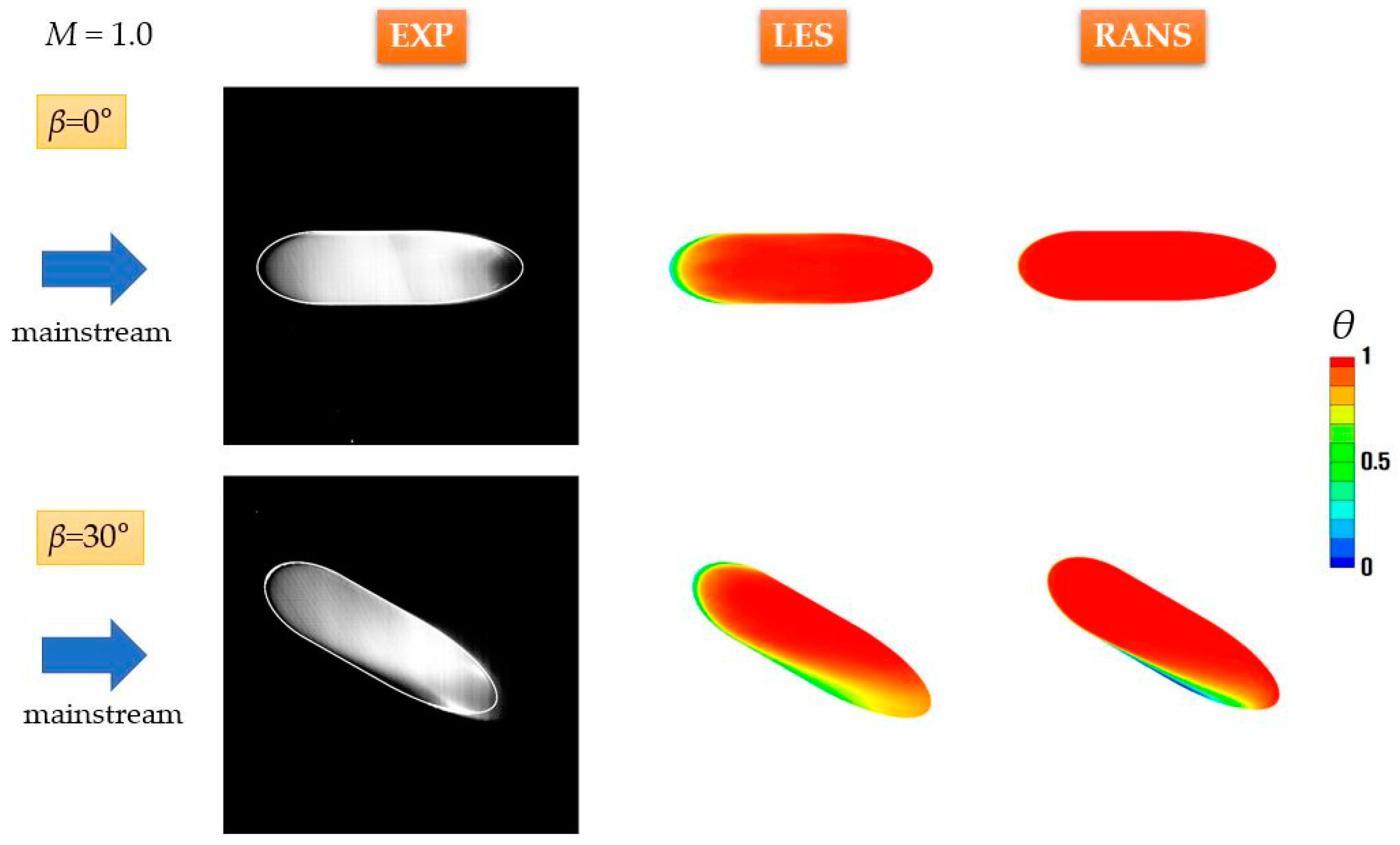
4.7. Mean Dimensionless Temperature Contours at Hole Exit

The cross-sectional area in the forward expansion hole was larger than that in the cylindrical hole, and the interaction between the hot main flow and coolant at the hole exit is complex [31]. Figure 20 and Figure 21 illustrate the contours of the time-averaged dimensionless temperature at the hole exit obtained with LES and RANS simulations for M = 0.5 and 1.0, respectively; these results were compared to the experimental flow visualization contours presented in [19]. The purpose of flow visualization is to determine the region in which the mainstream is ingested into the hole and to understand the interaction between the main flow and injectant at the hole exit [19]. After the coolant and oil aerosol had been mixed, it was illuminated by the laser sheet at the hole exit. The motion of the mixed injectant was captured by camera [31]. The dark color in the visualization contour indicates that the hot main flow was reversed in the hole, whereas the white color in the visualization contour indicates that the hot main flow was injected from the hole, corresponding with a non-dimensional temperature of 1 [19]. When the main flow is ingested into the hole, it could damage the hole owing to its high temperature. Moreover, the reversed flow can affect the film cooling performance downstream of the hole on the test plate [31]. Thus, it is important to know the area of hot main flow reversal. Compared to that of the flow visualization contours, the RANS contours show that the area in which the hot main flow was ingested into the hole is smaller than that of the LES results at M = 0.5 and 1.0. The flow visualization contours show the reversal of the flow in the hole around its leading edge; the LES results present this phenomenon for β = 0° and 30° well, while the RANS results indicate the occurrence of this phenomenon slightly. However, for β = 30°, the reversed flow around the upstream edge of the hole was observed in both RANS and LES results clearly. In the figures, for β = 0°, the reversed flow was generated only around the leading edge, while for β = 30°, the reversed flow was also generated around the upstream edge of the hole because the injectant with a high momentum near the leading edge cannot protect a low momentum region vulnerable to the hot main flow near the upstream edge of the hole when the compound angle (β) was 30° [31].

5. Conclusions

The film cooling process with a forward expansion hole with 0° and 30° compound angles at M = 0.5 and 1.0 was numerically simulated with LES and RANS simulations. Regarding the contours of the film cooling effectiveness on the wall, combining the compound angle of 30° and shaped hole promoted the lateral spreading of the coolant, leading to a more uniform coolant coverage and increased the spanwise-averaged film cooling effectiveness. RANS overpredicted the film cooling effectiveness in the narrow region near the hole; by contrast, the LES results and experimental data agree well. Thus, the local distribution of η in the spanwise direction based on RANS simulations did not agree well with the experimental data; however, the RANS simulation predicted the spanwise-averaged film cooling effectiveness well because it underpredicted lateral spreading of the coolant. Because the thermal damage on turbine blade surfaces is generated by poor local cooling, LES should be used to predict the local film cooling effectiveness instead of RANS. In the cross-sectional time-averaged dimensionless temperature contours, the dimensionless temperature of the coolant core area in the RANS results was higher than that in the LES results because the mixing intensity between the hot mainstream flow and injectant in the RANS results was not as high as in the LES results. Regarding the forward expansion hole, the overall velocity and temperature fluctuations in the LES contours were smaller than those of the cylindrical hole; thus, the turbulence and mixing intensity in the forward expansion hole were lower than those in the cylindrical hole, respectively. In particular, the velocity fluctuations in the normal direction for the forward expansion hole were greatly decreased compared to those of the cylindrical hole since the injection velocity in the normal direction was reduced by increased cross-sectional area at the forward expansion hole exit. The area with high θ_rms was larger than the area with high-velocity fluctuations. Additionally, for the forward expansion hole with β = 0°, the maximal θ_rms in the LES contour exceeded that for β = 30°; thus, the mixing intensity for β = 0° exceeded that for β = 30°; this resulted in a higher η on the wall for β = 30°. The flow visualization contours of the experiment and LES results clearly show the flow reversal around its leading edge in the forward expansion hole, whereas the RANS results did not show this phenomenon because the velocity of the injectant near the trailing edge of the hole was lower in the forward expansion hole than that in the cylindrical hole. Considering the reversed main flow into the hole can damage the hole and affect the film cooling performance downstream of the hole, it is important to know the area of hot main flow reversal accurately.

References

1. Moran, M.; Shapiro, H.; Boettner, D.; Bailey, M. Fundamentals of Engineering Thermodynamics, 8th ed.; Wiley: Hoboken, NJ, USA, 2014; p. 532. [Google Scholar]
2. Mai, T.D.; Ryu, J. Effects of leading-edge modification in damaged rotor blades on aerodynamic characteristics of high-pressure gas turbine. Mathematics 2020, 8, 2191. [Google Scholar] [CrossRef]
3. Leedom, D.H.; Acharya, S. Large eddy simulations of film cooling flow fields from cylindrical and shaped holes. In Proceedings of the ASME Turbo Expo 2008, Berlin, Germany, 9–13 June 2008; GT2008-51009. pp. 865–877. [Google Scholar]
4. Acharya, S.; Leedom, D.H. Large eddy simulations of discrete hole film cooling with plenum inflow orientation effects. J. Heat Transf. 2013, 135, 011010. [Google Scholar] [CrossRef]
5. Baek, S.I.; Ahn, J. Large Eddy Simulation of Film Cooling with Bulk Flow Pulsation: Comparative Study of LES and RANS. Appl. Sci. 2020, 10, 8553. [Google Scholar] [CrossRef]
6. Fujimoto, S. Large eddy simulation of film cooling flows using octree hexahedral meshes. In Proceedings of the ASME Turbo Expo 2012, Copenhagen, Denmark, 11–15 June 2012. GT-2012-7009. [Google Scholar]
7. Walters, D.K.; Leylek, J.H. Impact of film-cooling jets on turbine aerodynamic losses. ASME J. Turbomach. 2000, 122, 537–545. [Google Scholar] [CrossRef]
8. McGovern, K.T.; Leylek, J.H. A detailed analysis of film cooling physics: Part II—Compound-angle injection with cylindrical holes. ASME J. Turbomach. 2000, 122, 113–121. [Google Scholar] [CrossRef]
9. Tyagi, M.; Acharya, S. Large eddy simulation of film cooling flow from an inclined cylindrical jet. ASME J. Turbomach. 2003, 125, 734–742. [Google Scholar] [CrossRef]
10. Rozati, A.; Tafti, D. Large eddy simulation of leading edge film cooling: Part II—Heat transfer and effect of blowing ratio. In Proceedings of the ASME Turbo Expo 2007, GT2007-27690, Montreal, QC, Canada, 14–17 May 2007. [Google Scholar]
11. Johnson, P.; Shyam, V.; Hah, C. Reynolds-Averaged Navier–Stokes Solutions to Flat Plate Film Cooling Scenarios, NASA/TM-2011-217025. Available online: https://ntrs.nasa.gov/api/citations/20110012464/downloads/20110012464.pdf (accessed on 1 February 2021).
12. Goldstein, R.J.; Eckert, E.R.G.; Burggraf, F. Effects of hole geometry and density on three-dimensional film cooling. Int. J. Heat Mass Transf. 1974, 17, 595–607. [Google Scholar] [CrossRef]
13. Bell, C.M.; Hamakawa, H.; Ligrani, P.M. Film cooling from shaped holes. J. Heat Transf. 2000, 122, 224–232. [Google Scholar] [CrossRef]
14. Hyams, D.G.; Leylek, J.H. A detailed analysis of film cooling physics: Part III-Streamwise injection with shaped holes. J. Turbomach. 2000, 122, 122–132. [Google Scholar] [CrossRef]
15. Wang, C.; Zhang, J.; Feng, H.; Huang, Y. Large eddy simulation of film cooling flow from a fanshaped hole. Appl. Therm. Eng. 2018, 129, 855–870. [Google Scholar] [CrossRef]
16. Oliver, T.A.; Bogard, D.G.; Moser, R.D. Large eddy simulation of compressible, shaped-hole film cooling. Int. J. Heat Mass Transf. 2019, 140, 498–517. [Google Scholar] [CrossRef]
17. Wang, Q.; Su, X.; Yuan, X. Large-eddy simulation of shaped hole film cooling with the influence of cross flow. Int. J. Turbo Jet Eng. 2020. ahead-of-print. [Google Scholar]
18. Zamiri, A.; You, S.; Chung, J. Large eddy simulation in the optimization of laidback fan-shaped hole geometry to enhance film-cooling performance. Int. J. Heat Mass Transf. 2020, 158, 120014. [Google Scholar] [CrossRef]
19. Lee, H.W.; Park, J.J.; Lee, J.S. Flow visualization and film cooling effectiveness measurements around shaped holes with compound angle orientations. Int. J. Heat Mass Transf. 2002, 45, 145–156. [Google Scholar] [CrossRef]
20. ANSYS Fluent Theory Guide Version 19. Available online: https://www.ansys.com/products/fluids/ansys-fluent (accessed on 1 February 2021).
21. Pointwise Version 18. Available online: http://www.pointwise.com/ (accessed on 1 February 2021).
22. Baek, S.I.; Yavuzkurt, S. Effects of flow oscillations in the mainstream on film cooling. Inventions 2018, 3, 73. [Google Scholar] [CrossRef] [Green Version]
23. Renze, P.; Schröder, W.; Meinke, M. Large-eddy simulation of film cooling flows with variable density jets. Flow Turbul. Combust. 2008, 80, 119–132. [Google Scholar] [CrossRef]
24. Iourokina, I.; Lele, S. Towards large eddy simulation of film cooling flows on a model turbine blade leading edge. In Proceedings of the 43rd AIAA Aerospace Sciences Meeting and Exhibit, No. 2005-0670, Reno, NV, USA, 10–13 January 2005. [Google Scholar]
25. Ravelli, S.; Abdeh, H.; Barigozzi, G. Numerical Assessment of Density Ratio and Mainstream Turbulence Effects on Leading-Edge Film Cooling: Heat and Mass Transfer Method. J. Turbomach. 2021, 143, 041002. [Google Scholar] [CrossRef]
26. White, F. Fluid Mechanics, 8th ed.; McGraw-Hill: New York, NY, USA, 2015. [Google Scholar]
27. Ryu, J.; Lele, S.; Viswanathan, K. Study of supersonic wave components in high-speed turbulent jets using an LES database. J. Sound Vib. 2014, 333, 6900–6923. [Google Scholar] [CrossRef]
28. Choi, M.G.; Ryu, J. Numerical study of the axial gap and hot streak effects on thermal and flow characteristics in two-stage high pressure gas turbine. Energies 2018, 11, 2654. [Google Scholar] [CrossRef] [Green Version]
29. Oh, J.S.; Kang, T.; Ham, S.; Lee, K.S.; Jang, Y.J.; Ryou, H.S.; Ryu, J. Numerical analysis of aerodynamic characteristics of hyperloop system. Energies 2019, 12, 518. [Google Scholar] [CrossRef] [Green Version]
30. Le, T.T.G.; Jang, K.S.; Lee, K.S.; Ryu, J. Numerical investigation of aerodynamic drag and pressure waves in hyperloop systems. Mathematics 2020, 8, 1973. [Google Scholar] [CrossRef]
31. Lee, H.W. Effects of Bulk Flow Pulsations on Film Cooling with Shaped Holes. Ph.D. Thesis, Seoul National University, Seoul, Korea, 2000. [Google Scholar]
32. Lee, S.W.; Kim, Y.B.; Lee, J.S. Flow characteristics and aerodynamic losses of film cooling jets with compound angle orientations. J. Turbomach. 1997, 119, 310–319. [Google Scholar] [CrossRef]
33. Baek, S.I.; Ahn, J. Large eddy simulation of film cooling with triple holes: Injectant behavior and adiabatic film cooling effectiveness. Processes 2020, 8, 1443. [Google Scholar] [CrossRef]
34. Burd, S.W.; Kaszeta, R.W.; Simon, T.W. Measurements in film cooling flows: Hole L/D and turbulence intensity effects. J. Turbomach. 1998, 120, 791–798. [Google Scholar] [CrossRef] [Green Version]
Figure 1. Schematics of forward expansion hole configuration. D: diameter of the lower hole.
Energies 14 02063 g001
Figure 2. Computational domains of forward expansion holes.
Energies 14 02063 g002
Figure 3. Computational fluid dynamic (CFD) meshes of forward expansion hole with β = 0°: (a) mesh in x–y plane (b) mesh in y–z plane (c,e) close-up of mesh near the cooling hole, and (d) mesh at hole exit.
Energies 14 02063 g003
Figure 4. Spanwise-averaged effectiveness of forward expansion hole with β = 0° in grid sensitivity test with large eddy simulations (LES).
Energies 14 02063 g004
Figure 5. Spanwise-averaged effectiveness of forward expansion hole with β = 30° in grid sensitivity test with LES.
Energies 14 02063 g005
Figure 6. Time-averaged distribution of η at M = 0.5: (a) β = 0° and (b) β = 30°.
Energies 14 02063 g006
Figure 7. Distribution of time-averaged η at M = 1.0: (a) β = 0° and (b) β = 30°.
Energies 14 02063 g007
Figure 8. Cross-sectional time-averaged dimensionless temperature distributions at M = 0.5.
Energies 14 02063 g008
Figure 9. Cross-sectional time-averaged dimensionless temperature distributions at M = 1.0.
Energies 14 02063 g009
Figure 10. Contours of time-averaged dimensionless temperature and streamlines at x/D = 2.5 and M = 0.5.
Energies 14 02063 g010
Figure 11. Contours of time-averaged dimensionless temperature and streamlines at x/D = 2.5 and M = 1.0.
Energies 14 02063 g011
Figure 12. Spanwise-averaged film cooling effectiveness at blowing ratios of 0.5 and 1.0.
Energies 14 02063 g012
Figure 13. Time-averaged film cooling effectiveness at x/D = 5 for 0.5 blowing ratio.
Energies 14 02063 g013
Figure 14. Time-averaged film cooling effectiveness at x/D = 5 for 1.0 blowing ratio.
Energies 14 02063 g014
Figure 15. Contours of instantaneous film cooling effectiveness on wall obtained with LES: (a) β = 0°, M = 0.5; (b) β = 30°, M = 0.5; (c) β = 0°, M = 1.0; (d) β = 30°, M = 1.0.
Energies 14 02063 g015
Figure 16. Contours of turbulence intensities obtained with LES for x/D = 2.5 and M = 0.5.
Energies 14 02063 g016
Figure 17. Comparison of contours of turbulence intensities obtained with LES for x/D = 2.5 and M = 1.0 with experimental results presented in [34].
Energies 14 02063 g017
Figure 18. Contours of dimensionless temperature fluctuations obtained with LES at x/D = 2.5.
Energies 14 02063 g018
Figure 19. Mean velocity on x−y plane.
Energies 14 02063 g019
Figure 20. Mean dimensionless temperature compared with experimental flow visualization [19] at hole exit at M = 0.5.
Energies 14 02063 g020
Figure 21. Mean dimensionless temperature compared with experimental flow visualization [19] at hole exit at M = 1.0.
Energies 14 02063 g021