Weather Related Fault Prediction in Minimally Monitored Distribution Networks

Abstract

Power distribution networks are increasingly challenged by ageing plant, environmental extremes and previously unforeseen operational factors. The combination of high loading and weather conditions is responsible for large numbers of recurring faults in legacy plants which have an impact on service quality. Owing to their scale and dispersed nature, it is prohibitively expensive to intensively monitor distribution networks to capture the electrical context these disruptions occur in, making it difficult to forestall recurring faults. In this paper, localised weather data are shown to support fault prediction on distribution networks. Operational data are temporally aligned with meteorological observations to identify recurring fault causes with the potentially complex relation between them learned from historical fault records. Five years of data from a UK Distribution Network Operator is used to demonstrate the approach at both HV and LV distribution network levels with results showing the ability to predict the occurrence of a weather related fault at a given substation considering only meteorological observations. Unifying a diverse range of previously identified fault relations in a single ensemble model and accompanying the predicted network conditions with an uncertainty measure would allow a network operator to manage their network more effectively in the long term and take evasive action for imminent events over shorter timescales.

1. Introduction

Adverse weather conditions can have a significant impact on electricity network infrastructure and will subsequently compromise the quality of power delivered to consumers. A study on the effects of climate change on the US electrical network concluded that $80\%$ of all large scale power outages between 2003 and 2012 were caused by weather and the average number of weather related outages per year doubled during those years [1]. Although some results refer to weather conditions specific to the US climate, they are indicative of how changing weather conditions can affect the electricity network. In the UK, the distribution network operators have published climate adaptation reports, outlining the current risks and the anticipated impacts as a result of a changing climate. Among others, ref. [2] discusses the main results of a study conducted with the UK Met Office regarding the impacts on the electricity network, which identified the major causes of weather related outages and estimated how their frequency might change in the future. Using the Met Office climate projections [3], the study showed that there is an uncertainty regarding the future occurrence of wind related faults, as there is uncertainty in the wind gust projections as well. However, the number of lightning related faults is more likely to increase and the faults due to snow, sleet and blizzard are estimated to be fewer but with the same or increased intensity.

1.1. Overview of Research

This work examines the consequence of weather conditions on the distribution network operation and attempts to predict the occurrence of weather-related faults in the case where only weather observations are available. These are typical conditions for a UK distribution network, where little to no monitoring is usually available. In addition, this work was conducted with a UK Distribution Network Operator (DNO) and stemmed from expert observations that certain faults occurred following certain weather conditions, therefore it is an application with real operational value. Therefore, the methodology and predictive models from this research can be deployed immediately to offer value in a distribution network. There is no need for costly additional monitoring equipment installation. This is also achieved without detailed topographic information or widespread environmental sensing. The focus of this paper is on the prediction of weather related faults at the HV and LV level of a distribution network, considering only the fault history for that network and historical weather conditions. While weather is not the sole contributor to a distribution network’s faults, it has been proven from the relevant research (as discussed later in this paper) that it has a major impact on the power systems faults. This combined with the fact that weather data are usually more easily obtained (and with less cost) than component specific measurements led to the decision to address this issue using meteorological data only. The purpose of this work is not to predict the exact location of the fault or specific type of electrical fault, but the circuit that is more likely to be affected by a fault, given the expected weather conditions in that area. To this end, statistical analysis and machine learning methods are used, where the fault records are used as ground truth for the event occurrences in the network and minimal environmental data are examined as fault causes. The results presented and discussed later in this paper show that the prediction of a weather related fault at a specific part of a distribution network considering only meteorological observations is possible. A practical application stemming from the work presented in this paper would be utilising longer term weather forecasts in order to identify areas of the distribution network that might be at risk of fault under specific weather conditions. This can extend to both HV and LV levels of the network, where this methodology could be used to enhance preparedness for a fault potentially affecting a large number of customers or strategically position maintenance staff, therefore assisting in the overall distribution network management. The uncertainty measure associated with the predictions would allow the DNOs to act on predictions according to their attitude to risk. The data analysis methodology presented in this paper can be summarised in Figure 1.

The diagram shown in Figure 1 gives an overview of how the weather variables are analysed in conjunction with the fault records in order to identify a suitable fault prediction model. The different stages of the methodology from the dataset development to the selection of the fault prediction model of Figure 1 are detailed in Section 2 and Section 3 of this paper, which discuss the data used and the data analysis process, respectively.

1.2. Related Work

The weather related impacts on the power system and the uncertainties accompanying climate change have been a recurring research subject of the academic and power industry sectors. The existing research on weather related fault prediction is reviewed in this section, which concludes with the contribution of the work presented in this paper and how it differs from the previously conducted research.

A review of the research addressing the impacts of extreme weather on the power systems’ resilience is presented in [4], where a framework for the modelling of weather related impacts on power systems is proposed. A methodology based on this framework is developed in [5], where the effects of windstorms on the transmission network’s resilience are assessed, utilising real time weather conditions and calculating the weather dependent failure probabilities. The application of this methodology on the GB transmission network determined the critical wind speed above which there was a sharp increase in the event occurrences per year.

The effect of wind on the GB transmission system was also investigated in [6], where historical data was used to identify the relationship between wind gust and fault occurrence. The work presented in this paper concluded that, when extreme values of wind gust are observed there is a higher probability for a wind related fault to occur. The occurrence, intensity and duration of wind storms in the northeast US are modelled in [7]. Subsequently, the dependencies of weather and component failure are investigated, and the risk of failure is quantified for the components of a real distribution system.

Weather data have been used as part of an improved protection strategy called hierarchically coordinated protection [8,9]. Unlike other fault prediction approaches which aim to prevent the occurrence of a fault, the purpose of prediction in hierarchically coordinated protection is to give the utilities the opportunity to anticipate a weather-related fault and be better prepared to deal with it. This approach utilises weather data and machine learning techniques such as Neural Networks or Support Vector Machines to detect and classify the potential faults. Then, when a fault is detected and recognised by the system, the protection is adjusted based on the type of the fault. The prediction of occurrence and location of weather-related faults in the distribution network was also examined in [10] which provides a comparison of machine learning models developed for this purpose. Again, the aim of these predictive models, which utilised grid electrical parameters and infrastructure type alongside historical weather and fault data, was to enhance preparedness for an event rather than preventing it.

The use of historical weather data alongside a number of other data sources such as customer calls and Smart Meter data, geographical information system data, asset condition data etc, for post fault analysis is proposed in [11]. Work utilising the above ideas is presented in [12,13], where historical and real time weather data are analysed alongside data from various other sources in order to provide an understanding of the effects that different nature-caused events have on the network and produce risk maps for weather-related outages using a geographical information system framework and fuzzy logic, respectively.

Weather conditions and lightning strike positions have been used in addition to data from remote power quality monitoring devices to improve their predictive maintenance system by detecting incipient equipment failure in [14], while in [15] wind speed data in conjunction with component resiliency index and distance from the hurricane centre have been used as inputs to a Support Vector Machine model, in order to predict an electrical grid component outage following a hurricane.

Data from maintenance tickets, features related to equipment vulnerability and various weather-related features, mostly related to temperature and precipitation to model monthly weather conditions have been used for the modelling approach presented in [16]. The aim of this model was to gain an insight of the weather factors that significantly affect the power grid and, subsequently, lead to serious events and model their dependencies.

A framework to predict the duration of distribution system outages is presented in [17]. Using outage reports and their respective repair logs in conjunction with weather data, it was found that certain weather features were correlated with specific causes and good results could be achieved, even when taking only weather data into account. The inclusion of information contained in the outage reports and repair logs was found to enhance the model’s performance.

An analysis of the correlation between failures and weather conditions is presented in [18], where market basket style analysis is used to generate predictive rules using weather data which has been earlier categorised as “high”, “medium” or “low”. The analysis gave a moderate accuracy of prediction but indicated that there is potential in using weather forecasts to predict component failure. In [19], an extended version of logistic regression is used to perform a probabilistic classification and calculate the probability of a fault occurrence given information regarding the weather conditions, location, time and operating voltage.

The relationship between weather conditions and the total number of interruptions is examined in [20], where historical weather data and daily number of failures are considered in order to predict the total number of weather related failures in a year. The purpose of this work is to assess the network’s performance by the end of the year by comparing the actual and the previously predicted number of failures. Similar work is presented in [21], where a Neural Network based model is developed to predict the total number of interruptions and not only those that are directly caused by weather conditions.

The previously conducted research presented above, gives an idea of how weather data have been used to predict weather related faults for various applications. The first examples of research work discussed, refer to fault prediction at the transmission level and wind is the environmental factor that is predominantly considered. Next, the relevant work at the distribution level was discussed. The majority of this work utilises a substantial amount of data, coming from various sources alongside the weather data that they use. Two of the papers presented above [20,21], make use of weather data and number of failures only but their purpose is to predict the total number of interruptions in a region. 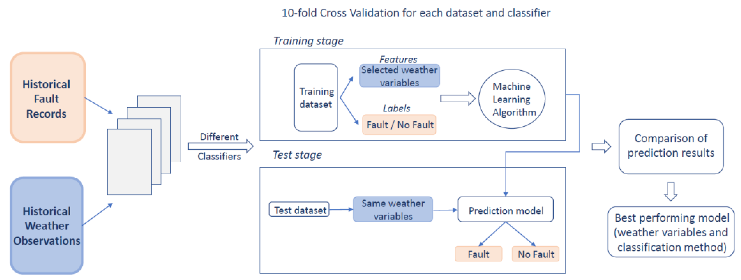Another [18], aims to predict a component failure using only weather data but, instead of using the actual measurements, they have previously classified them in three categories (high, medium, low). In contrast, the research work presented in this paper aims to assess the impact of weather on the occurrence of distribution network faults in the absence of extensive monitoring. As the distribution networks in the UK are usually minimally observed, this work utilises already existing meteorological data from local Met Office weather stations and fault records provided by a UK Distribution Network Operator, in order to predict a weather related fault occurrence at a given location. This work extends the fault prediction methodology down to the LV level of the distribution network and follows an ensemble approach, which unifies a range of identified fault relations as these were captured by a number of machine learning methods, allowing the benefits of different techniques to be combined in a single model. The machine learning methods used in this paper have already been used in the literature to address various applications and no new techniques are proposed as part of this paper. The motivation for using machine learning was to address the unknown physics of the individual fault cause processes. Identifying the most suitable methods for this specific task and combining them in an ensemble model that retains the strengths of individual models results in the development of fault prediction models for the HV and LV distribution network that can have a significant impact from a practical point of view.

The remainder of this paper is organised as follows. The network operator data and context are described in Section 2. In Section 3, the machine learning methods and the data analysis process are described, while the results are presented and discussed in the three case studies of Section 4. Finally, a brief summary and conclusion discussing the operational benefit of this research are given in Section 5.

2. Network Operator Data and Context

The work presented in this paper utilises fault data from a real distribution network alongside historic weather observations. This section provides an overview of the context and nature of the data used.

2.1. Fault Records

Five years of fault records were provided by Northern Powergrid (NPG) and used for the work presented in this paper. The data files contained the recorded incidents that occurred at both the HV and LV levels of their distribution network (covering the areas of North East of England, Yorkshire and northern Lincolnshire) and were examined first separately and then together.

The HV fault records cover the period 20 May 2013–20 July 2018 and contain 17,653 events in total. The range of voltages covered in the HV fault records was $6.6$ kV–132 kV with the majority of recorder faults occurring at 11 kV (~76%) followed by 20 kV (~18%), which is reasonable as the largest part of NPG’s distribution network operates in these levels. The postcode of the incident location was available in the report description for 16,318 of these faults, with 2441 of them being weather related faults (based on the cause registered in the fault records). The causes included in the weather related faults and the number of events per cause are listed in

Table 1. HV weather related faults.

Cause	No. of Events	Customers Affected (Median)	Total CML (Median)
Wind and Gale (excl. Windborne Material)	1023	82	12,243
Lightning	902	20	4439
Snow, Sleet and Blizzard	204	133	21,655
Windborne Materials	133	49	10,109
Flooding	70	8	3088
Ice	34	58	9009
Rain	34	163	15,962
Solar Heat	25	62	4595
Freezing Fog and Frost	16	64	7871

, which also states the median number of customers affected and the median Customer Minutes Lost (CML) that correspond to the faults that belong to each of the weather fault causes considered.

The locations of the faults on Northern Powergrid’s HV network can be seen in Figure 2, where the size of the circles corresponds to the number of customers affected by each event and the colour to the total CML. The darker colour of the circles indicates lower CML. According to Ofgem [22], all interruptions with durations of 3 min or longer contribute to a fault’s CML. In this paper, the CML is used to explain the impact of weather related faults and how this differs in the different voltage levels.

A histogram of the CML that corresponds to each of the HV recorded faults can be seen in Figure 3.

Figure 3 demonstrates that the majority of faults have low CML, reflecting a short duration and/or a small number of affected customers-at HV this is more likely to be the former. The LV fault records cover the period 16 June 2013–11 June 2018 and contain 103,819 events in total. The LV faults refer to the LV side of the secondary transformer ($0.4$ kV). The postcode of the incident location was available in the report description for 60,501 of these faults, with only 711 of them being weather related faults. The number of events per weather related cause for the LV level, the number of customers affected and the CML for each fault are shown in

Table 2. LV weather related faults.

Cause	No. of Events	Customers Affected (Median)	Total CML (Median)
Wind and Gale (excl. Windborne Material)	476	2	594
Rain	132	1	260
Flooding	64	6	1190
Solar Heat	16	1	60
Snow, Sleet and Blizzard	10	2	604
Lightning	8	4	915
Windborne Materials	5	3	625

. It can be seen that no faults due to “Ice” or “Freezing Fog and Frost” are present at the LV level, which is probably due to the fact that it is a predominantly underground network.

Unlike the HV level, where the numbers of weather, non-weather and unknown cause faults were comparable, this is not the case for the LV level, where the amount of faults with a registered weather cause is significantly lower than the rest. It is worth noting that even when including the 43,318 LV incidents, for which no postcode was available (and were not included in the analysis), the number of events that have been registered as weather related faults is only 1034 which is still very low compared to the total amount of LV faults. This, combined with the fact that the number of unknown cause faults at the LV level is very high, could be an indication that weather related faults at LV level are underestimated as they cannot always be correctly identified. The fault occurrences and their locations for the LV level can be seen in Figure 4 and a histogram of the CML that corresponds to each of the LV recorded faults can be seen in Figure 5. The ratio of customers affected at HV and LV level has been taken into account so that the sizes of the circles appearing on the map are of the same order of magnitude. The visualisation of the fault data on the map serves two purposes. First, it provides an easy way of assessing the impact of weather related faults and identify areas of the network that are affected more by this type of faults. In addition, the ratio of weather related faults with respect to the total number of faults indicates where there is a greater need for a weather related fault prediction. It is worth noting, that although the number of fault occurrences is much higher at the LV level, the HV faults are more valuable to predict as there are more customers per substation at the HV compared to the LV level. Therefore an HV fault results in higher CML.

Figure 5 shows a similar distribution to Figure 3, in that the majority of faults have a low CML; unlike HV, the distribution tail is heavier, indicating the potential for longer (although with fewer customers affected) CML from weather related faults-this may be exacerbated by the lack of automation on distribution networks, necessitating manual restoration of power or replacement of damaged components.

It is worth noting that the effects of weather on the distribution network can vary significantly. Certain weather conditions can have an immediate effect that would result in a fault (short term fault cause) or can have a cumulative effect, leading to asset degradation and failure at a later date (long term fault cause). This would affect the assets’ Health Index which would subsequently influence the resulting CML [23].

2.2. Weather Data

For the purposes of this analysis, access to the Met Office UK MIDAS datasets was granted by the Centre of Environmental Data Analysis (CEDA). Nineteen weather variables were considered for the analysis and are shown in

Table 3. Fault predictive weather variables.

	Variable	Units
1	Precipitation on the day before	mm
2	Sum of precipitation 2 days before	mm
3	Sum of precipitation 3 days before	mm
4	Sum of precipitation 6 days before	mm
5	Max daily air temperature	deg C
6	Min daily air temperature	deg C
7	Difference in max air temperature with day before	deg C
8	Difference in min air temperature with day before	deg C
9	Mean wind speed	knots
10	Mean wind direction	deg (true)
11	Max gust speed	knots
12	Max gust direction	deg (true)
13	Air temperature	deg C
14	Dew point temperature	deg C
15	Wet bulb temperature	deg C
16	Humidity	%
17	Derived hourly sunshine duration	0.1 h
18	Total cloud amount code	eighths
19	Visibility	dam

. The total number of active Met Office weather stations within NPG’s licence area is 276. Not all measurements are available at each weather station, so data from more than one station was used to describe the weather conditions at the time of a fault. The 19 variables are categorised in 4 groups of weather data: daily rainfall (RD), daily temperature (TD), hourly wind (WM) and hourly weather observations (WH). To obtain the desired data, the locations of all active weather stations within Northern Powergrid’s licence area were compared to the known fault locations (postcode found in each fault’s ‘location text’ description in the fault records) and a nearest weather station for each group of variables was assigned to each fault. These measurements were then used to form the datasets that are discussed later in the paper.

The measurements used for the variables (1)–(8) were recorded on a daily basis, while hourly measurements were used for the rest of the variables. There were two reasons why daily precipitation data was selected over hourly. Based on the network owners experience, in the case of an underground fault at both HV and LV levels, the rainfall in the days before the event has a greater impact than at the time of the event, as it takes some time for the rainfall to permeate through the ground into the cables that have been damaged by the ground movement. This is not the case for flooding events, when the faults occur fairly soon after the rain. However, since there are more Met Office weather stations collecting daily precipitation data compared to those collecting hourly, and it was possible to use data from a site nearer to the fault location, daily precipitation data was chosen for this analysis. The timescales of the selected weather variables that are used as inputs to the classification models with respect to the time of the fault (or no fault) example can be seen in Figure 6.

Using the information available for the weather related faults and the weather measurements for the corresponding periods, a new dataset was created for each voltage level. These new datasets contained weather variables describing the conditions for Fault and No Fault examples and were used as inputs to the classifiers, which are described in the next section. The dates and times of the Fault examples were taken directly from the fault records. In our analysis, anything that results in the interruption of power supply is considered a Fault, while a No Fault example can be any time when no fault occurred, i.e., there was no fault record present. For each of the recorded faults, two No Fault examples were selected for the same location. The time of the first No Fault example was selected to be 24 h before the fault (previous day, same time) and the time of the second No Fault example was one week before the fault (one week before, same day, same time). This was done to ensure that the fault was not caused by a typical time based network event. If a selected date and time for a No Fault example coincided with a date and time of a fault in the fault records, then it was not included in the analysis. After the dates and times were finalised, the corresponding values for the selected weather variables were extracted from the nearest weather station corresponding to each of the 4 groups of variables mentioned earlier in this section. The day ahead prediction model uses two major sets of inputs to create its forecast of faults: the relevant weather conditions up to one week before (the timescales for each weather variable considered are shown in Figure 6); and, the weather forecast for the next day. If a longer term prediction of faults is required, then long-range weather forecasts can be used and the predictions updated as weather forecasts change closer to the period when the fault prediction is required.

As the measurements for the selected weather variables were not available for all dates and times in the new dataset, a number of different subsets were explored, including different combinations of weather variables and Fault/No Fault examples each time. These subsets, which had different sizes, were then used as inputs to the classifiers for a comparison in order to identify the best performing method, based on the criteria outlined in Section 3. The datasets resulting from the process discussed above, describe the training and test datasets used later in the paper. A more detailed presentation of the process described above and how this work fits in a more general data analysis methodology for distribution networks can be found in [24].

3. Application of Data Analysis Methodology

This section is divided into two subsections, which describe the classification methods compared in this paper and the overall data analysis process.

3.1. Classification Methods

The main challenge is the need to accurately map environmental conditions to fault occurrence. The functional form of this relation will vary across networks, so a means of articulating it for all eventualities must possess a flexible decision surface that can be learned from past observations. To determine the optimal model choice, a selection of candidate classification techniques with diverse underlying decision surfaces were compared in order to identify the most suitable methods to classify exemplar data into: (a) Fault and No Fault and (b) No Fault and Fault Type. The characteristics of each of the methods considered in this paper are summarised in

Table 4. Characteristics of classification methods.

Classifier	Description	Advantages	Disadvantages	Decision Boundary
Classification and Regression Trees (CART)	One of the most established and commonly used classifiers. It works by partitioning data into rectangular boxes with bounding rules forming a decision tree. The tree is then used to predict the class of new, previously unseen, data examples [25].	Simple classifier, interpretable as a decision tree.	Functionally limited, prone to overfitting	Rectangular boxes
Naïve Bayes (NB)	Based on the Bayes Theorem and uses the probabilities of each feature for each class to make a prediction with the ‘naive’ assumption that observations are completely independent given the class label. The assumption of independence simplifies the calculation of the joint probability of the attributes for this class and, then, the class with the highest probability is selected [26].	Does not require large amount of training data. Fast compared to more sophisticated methods.	Assumption that predictors are completely independent.	Linear
Logistic Regression (LR)	A linear machine learning model that uses the logistic sigmoid function to estimate a probability value from the training data, which is then assigned to the relevant class to make a prediction [27].	Simple and easy to implement. Can be easily updated to incorporate new data.	Sensitive to outliers. Difficult to capture complex relationships	Linear
Support Vector Machines (SVM)	They construct a hyperplane that separates the data into their classes. The best separation can be generally achieved when the distance of the nearest points of each class to the hyperplane is greatest. For non linearly separable data, SVMs take this concept a step further by first mapping input variables into a high dimensional space to provide greater discriminative power [28]	Versatile and memory efficient method.	Large datasets required to train the SVM. Do not directly provide probability estimates	Linear or nonlinear. Nonlinear boundary used here (Radial Basis Function (RBF) kernel)
k-Nearest Neighbours (k-NN)	Uses a metric such as Euclidean distance to apportion labels to new data points based upon the labels of the k nearest data points [29].	Easy to understand and implement. No parameters to tune.	Memory intensive. Sensitive to noise.	Nonlinear
Gradient Boost Machines (GB)	Use multiple single predictors (often trees or rules) to make very simple, broad classifications and then weigh outputs from these according to their expected error into an overall classifier that has greater predictive power than any one of the constituent predictors [30].	Effective on wide area if applications. Flexible–allows to optimise user preferred loss functions.	Computationally expensive, not easily interpretable.	Can learn complex nonlinear decision boundaries.
Bagged Trees (BT)	Bagging is applied on a decision tree classifier. This means that the classifier is trained on random subsets (drawn with replacement) of the original training dataset and the final prediction is constructed by aggregating the individual predictions [31].	Improved accuracy compared to a single decision tree.	Can be computationally expensive.	Similar but smoother decision boundaries compared to CART.
Random Forest (RF)	Modified version of bagged trees, where many trees with reduced correlation are developed and then averaged [30].	Flexible, can fit a variety of data well.	Slow at training. Not suitable for small samples.	Similar to BT
Linear Discriminant Analysis (LDA)	Uses a linear boundary implied by the intersection of probability distributions representing difference classes. In LDA, a simplifying assumption is that classes have the same covariance structure [30].	Fast classification, easy to implement. Inherently multiclass classifier.	Can only learn linear boundaries.	Linear
Quadratic Discriminant Analysis (QDA)	QDA is similar to LDA but it differs in that it relaxes the assumption that classes have the same covariance, resulting in class decision boundaries that are quadratic [30].	More flexible than LDA, as it is not limited to a linear decision boundary.	More parameters to estimate.	Nonlinear (quadratic)
Multi-Layer Perceptron (MLP)	Neural Networks allow arbitrary nonlinear functions to be modelled either as regressors or classifiers. This is enabled by layers of hidden weights that are tuned to map model inputs to outputs through a process called Backpropagation [32]. The MLP that is used here is a basic type of feedforward neural network that is trained using the backpropagation algorithm to obtain parameter estimates.	Can learn nonlinear models. Can learn models in real time.	Sensitive to feature scaling. More than one local minima (in loss function) can lead to different validation accuracy for different random initialisations.	Nonlinear
Gaussian Process Classifier (GPC)	A Gaussian Process is a collection of random variables whose functional relation is represented as the covariance function of a multivariate Gaussian distribution. A GPC can take a number of decision surface shapes. It achieves this by modelling decision boundaries as a Multivariate Gaussian distribution with position dictated by its mean and decision threshold by is covariance function-this can be specified via a kernel function to take a different form along the length of the decision boundary [33].	Probabilistic prediction. Versatile-different kernels can be specified.	Efficiency decreases with higher dimensions.	Nonlinear

, while a brief description of how the two best performing classifiers work is given as follows.

Gradient Boost (GB): In machine learning, boosting is a method that combines many simple models in an ensemble that performs better than the individual models, by sequentially applying a weak classifier to repeatedly modified versions of the data. The first successful implementation of boosting was the AdaBoost algorithm, which is short for adaptive boosting. GB, which is a generalisation of AdaBoost, uses multiple single predictors (often trees or rules) to make very simple, broad classifications and then weighs outputs from these according to their expected error into an overall classifier that has greater predictive power than any one of the constituent predictors [30]. The classification process starts with a very simple model (e.g., a decision tree), which is a weak classifier, meaning that it produces predictions which are only slightly better than guessing. Then subsequent models are used to predict the error made by the model so far. The models, which are trained sequentially, focus on the difficult to predict data examples. The objective of these classifiers is to minimise the loss, which is the difference between the actual and the predicted class value of a training example. To minimise this loss, this method uses gradient descent.

Gradient Boost identifies the difficult to predict examples using residuals, which are calculated in each iteration m (and for each class k) using Equation (1). The difficult to predict data examples are identified by large residuals.

$$r_{k,im}=-{\left[\frac{\partial L(y_i,f_k\left(x_i\right))}{\partial f_k\left(x_i\right)}\right]}_{f_k=f_{k,m-1}}$$

(1)

where $L(y,f(x\left)\right)$ is the loss function.

The residuals are then used to train a weak classifier $h_{km}\left(x\right)$ which is multiplied by a multiplier ${\gamma }_{km}$. This is calculated using:

$${\gamma }_{km}=\underset{\gamma }{argmin}(\sum _{i=1}^{N}L(y_i,f_{k,m-1}\left(x_i\right)+\gamma h_{km}\left(x_i\right))$$

(2)

In the above equation, gradient descent is used to find the $\gamma$ that minimises this expression. The model is then updated to

$$f_{k,m}\left(x\right)=f_{k,m-1}\left(x\right)+{\gamma }_{km}{h}_{km}$$

(3)

This process is repeated K times at each iteration m, one for each class and the final model is given by K different (coupled) tree expansions $f_{kM}$, where $k=1,2,\dots ,K$, which produce the probabilities that a data point $x_i$ belongs to each of the K classes, as explained in [30].

Linear Discriminant Analysis (LDA): To make predictions, LDA as the name suggests, uses a linear decision boundary implied by the intersection of probability distributions representing difference classes [30]. A linear separation of the data is achieved when the data points are separated by class using a line or a hyperplane in the d dimensional input variable space. LDA finds a linear combination of input variables and the high dimensional data points are then projected on this eigenvector. Then, a hyperplane perpendicular to this vector is used as the linear decision boundary used for data classification (LDA can also be used for dimensionality reduction like PCA). In LDA, two simplifying assumptions about the data are made: (i) the data are assumed to follow a Gaussian distribution and (ii) the inputs of every class have the same covariance. A brief explanation of LDA for the case of binary classification of a high dimensional data point $\overrightarrow{x}=[x_1,x_2,\dots ,x_d]$, where each data point $\overrightarrow{x}$ belongs to one of two classes, namely $y=0$ or $y=1$, is given below.

To perform classification, LDA assumes that the conditional probability density functions of the two classes $p\left(\overrightarrow{x}\right|y=0)$ and $p\left(\overrightarrow{x}\right|y=1)$ follow a normal distribution. The mean vectors and covariance matrices of these distributions are assumed to be $(\overrightarrow{{\mu }_0},{\sum }_0)$ and $(\overrightarrow{{\mu }_1},{\sum }_1)$, respectively. Based on the above, a data point $\overrightarrow{x}$ belongs to the second class (here $y=1$) if the log of the likelihood ratio is bigger than some threshold T, so that:

$$\begin{array}{ccc}\hfill {(\overrightarrow{x}-\overrightarrow{{\mu }_0})}^T{\Sigma }_0^{-1}(\overrightarrow{x}-\overrightarrow{{\mu }_0})+ln\left|{\Sigma }_0\right|-& & \hfill \\ \hfill {(\overrightarrow{x}-\overrightarrow{{\mu }_1})}^T{\Sigma }_1^{-1}(\overrightarrow{x}-\overrightarrow{{\mu }_1})-ln\left|{\Sigma }_1\right|& >& T\hfill \end{array}$$

(4)

After the application of the second assumption of LDA, which is that the classes have common covariance matrices (${\Sigma }_0={\Sigma }_1=\Sigma$), the above expression is simplified and the decision criterion becomes a threshold on the dot product

$$\overrightarrow{w}·\overrightarrow{x}>c$$

(5)

where $\overrightarrow{w}={\Sigma }^{-1}(\overrightarrow{{\mu }_1}-\overrightarrow{{\mu }_0})$ and c is some threshold constant given by

$$c=\frac{1}{2}(T-{\overrightarrow{{\mu }_0}}^T{\Sigma }^{-1}\overrightarrow{{\mu }_0}+{\overrightarrow{{\mu }_1}}^T{\Sigma }^{-1}\overrightarrow{{\mu }_1})$$

(6)

In terms of classification of a data point $\overrightarrow{x}$ to one of the two classes, it is determined by which side of a hyperplane (that is perpendicular to $\overrightarrow{w}$) this point is located on. The threshold c determines the location of the above hyperplane.

The tradeoff to be made, when comparing the different methods, is one of complexity versus generalisation: the relation between fault occurrence and complex weather phenomena may not be captured by a simple classification boundary. However, closely fitting a classification boundary to very specific weather conditions is also undesirable as the classifier will capture too few eventualities-this phenomenon is referred to as overfitting [32].

Apart from the individual classification methods that were described in this section, two additional ensemble methods were used in the analysis presented in this paper. Ensemble methods provide a means of unification of a diverge range of identified fault relations in a single model. Two types of ensemble models were considered in this analysis: Voting and Stacking. A Voting classifier works by taking the outputs of a set of estimators (other classification methods) and calculating its output using ‘hard’ or ‘soft’ voting. Hard voting is based on the ‘majority rule’ meaning that the voting classifier outputs the label that was assigned to an example by a majority of estimators, while soft voting takes into account the probability of prediction along with the label assigned by each estimator. A Stacking classifier uses the outputs of the individual estimators as inputs to a final estimator in order to produce its prediction, allowing the strengths of each estimator to be reflected in the final prediction.

3.2. Data Analysis Process

The classification methods presented in Section 3.1 were applied to the data in order to do a classification between Fault and No Fault examples. Using a 10-fold cross validation approach, all the classifiers were applied on the same datasets and compared to find the ones that performed better. In cross validation, the dataset is split into a number of smaller subsets, which is 10 in this case. Out of these 10 subsets, 9 are used as the training set and 1 is used as the test set. This process is repeated 10 times so that all data points have been used for both training and testing. For datasets with an adequate number of faults for more than 1 weather related cause, the same process was used to classify the data between No Fault and each fault type. This process is repeated for the different datasets in order to obtain the final results of the best performing dataset and classification method, which determine the optimal model choice. The metrics used to assess the classification performance of each method were the classification accuracy, precision and recall and are computed using the expressions shown in

Table 5. Classification performance metrics.

Metric	Expression
Accuracy	$\frac{TP+TN}{TP+TN+FP+FN}$
Precision	$\frac{TP}{TP+FP}$
Recall	$\frac{TP}{TP+FN}$

, where TP is true positive, TN is true negative, FP is false positive and FN is false negative.

In the context of fault prediction, precision refers to the ability of the classifier not to label a No Fault as a Fault example, while the recall refers to its ability to find all Fault examples. Using these metrics, the overall performance of a classification method on each of the developed datasets is assessed and compared to that of the other classifiers. The ‘optimal model choice’ refers to selecting the model with the highest classification accuracy, precision and recall, while taking into account both the input variables (as different datasets have different combination of weather variables) and the classification algorithm. After applying the different classification methods to the different datasets at the HV and LV level separately, the best performing models were combined into two ensemble classifiers in order to assess their performance on a single dataset containing faults that occurred at both HV and LV distribution levels.

4. Results and Discussion

The process of jointly analysing distribution network fault data and historic weather data in order to predict the occurrence of weather related faults was described in the previous section. The results of this analysis are presented in the form of the following three case studies.

4.1. Weather-Related Fault Prediction at the HV Level

Section 2 describes the subsets of data considered which contain a different number of Fault/No Fault examples and part of the weather variables shown in Table 3. The dataset characteristics and the accuracy of the best performing classifier for each of these subsets are summarised in

Table 6. Summary of results for HV datasets.

Dataset	Weather Variables	Dataset Size	Accuracy	Classifier
#1	All	86 examples	$0.728$$\left(0.130\right)$	RF
#2	Excluding variable (17)	277 examples	$0.764$$\left(0.174\right)$	LDA
#3	(1)–(16)	381 examples	$0.792$$\left(0.156\right)$	LDA
#4	(1)–(4) and (9)–(16)	717 examples	$0.743$$\left(0.165\right)$	LDA

.

The numbers shown in the “Weather Variables” column in Table 6 correspond to the weather variable numbers in Table 3 and the values in the “Accuracy” column are the mean and standard deviation (in parentheses) accuracy resulted from the cross validation process. The accuracy refers to the accuracy of prediction of a fault at a given location given the weather conditions at the time of the fault and the days before the fault. The above results show that Linear Discriminant Analysis performed better in the majority of the analysed datasets, while the highest accuracy was achieved when dataset #3, which contained 381 Fault/No Fault examples, was used as input to the classifier. More detailed results regarding the analysis of this subset are presented below.

The 12 classifiers described in Section 3 were compared in order to find which of them performed better in this case study. The result of this comparison for the Fault/No Fault classification on dataset #3 is shown in Figure 7, which shows the range of the fault prediction accuracies for each classifier and

Table 7. Cross validation accuracy and standard deviation for HV dataset #3.

Classifier	Mean Accuracy	Standard Deviation
CART	$0.648$	$0.126$
NB	$0.761$	$0.145$
LR	$0.782$	$0.161$
SVM	$0.638$	$0.057$
KNN	$0.706$	$0.171$
BT	$0.711$	$0.134$
GB	$0.719$	$0.136$
RF	$0.743$	$0.113$
LDA	$\mathbf{0}.\mathbf{792}$	$\mathbf{0}.\mathbf{156}$
QDA	$0.755$	$0.162$
MLP	$0.677$	$0.159$
GPC	$0.683$	$0.130$

which shows the mean and standard deviation of the resulting accuracies for each classifier for dataset #3.

The majority of faults in this dataset were caused by “Wind and Gale” or “Lightning”, while only 7 faults were caused by other conditions. In order to explore the potential of the classifiers to classify the data not only into Fault and No Fault but also into the fault types, these 7 faults were removed from the dataset and the classification process was repeated for the reduced dataset. The results of this analysis were similar to those shown in Figure 7, with the mean classification accuracy for the best performing classifier (LDA) being $0.792$. To assess the classification results, metrics such as the precision and recall were considered alongside the classification accuracy. The meaning of these metrics was discussed in Section 3.2.

After removing the 7 Fault examples mentioned above, $80\%$ of the remaining dataset was used for training and $20\%$ for testing. Using LDA, which was the best performing classifier, the classification results on the held-out test set (48 No Fault and 27 Fault examples) are shown in Figure 8a, which shows the confusion matrix for this classification’s results and the relevant performance metrics.

It can be seen that, for this randomly chosen test set, the overall classification accuracy when using LDA is $86.67\%$. The model correctly classified 44 out of the 48 No Fault examples and 21 out of 27 Fault examples. Even though there are more Fault than No Fault examples that were misclassified, the accuracy is high considering the fact that only weather variables have been used to predict the occurrence of a fault. The same process was repeated in order to classify the faults based on their cause and the results are shown in Figure 8b.

Again, the overall classification accuracy is $86.67\%$ and 44 out of the 48 No Fault examples have been correctly identified. Regarding the fault causes, the model correctly classified 9 out of 10 faults caused by lightning and 12 out of 17 of those caused by wind. It is worth noting that no Fault example was attributed to the wrong cause as all the misclassified Faults were classified as No Faults. The results presented above show that it is possible to predict the occurrence of a weather related fault with a relatively high accuracy, considering only common weather variables that are not specific to a certain fault cause. From a network operator’s point of view, this work could be extended to make use of weather forecasts covering their licence area in order to identify potential fault locations ahead of time. Such an analysis could provide the opportunity for DNOs to identify vulnerable areas of their network and, therefore, be better prepared to respond to potential weather related faults.

4.2. Weather-Related Fault Prediction at the LV Level

As seen in Section 2, the LV faults with a registered weather related cause are fewer than those at HV level, even though a much higher number of faults occurred at the LV network. This combined with the lack of location information associated with many of the LV faults resulted in considerably smaller datasets. The results for the best performing classifier for the LV datasets are summarised in

Table 8. Summary of results for LV datasets.

Dataset	Weather Variables	Dataset Size	Accuracy	Classifier
#2	Excluding variable (17)	50 examples	$0.820$$\left(0.227\right)$	GB
#3	(1)–(16)	95 examples	$0.797$$\left(0.188\right)$	NB
#4	(1)–(4) and (9)–(16)	205 examples	$0.758$$\left(0.183\right)$	LR

. As there were only 9 Fault/No Fault examples with available data for all 19 weather variables, the LV equivalent to the #1 dataset is not included in this table.

During the LV fault analysis, the best performing dataset was found to be #2, which contained 50 Fault / No Fault examples. It is worth noting that the accuracy of prediction is also relatively high when datasets #3 and #4 are considered. The comparison of the results, however, indicates that the increased number of weather variables considered in dataset #2 gives a better description of the weather conditions affecting the LV network operation and, therefore, help to identify the most suitable prediction model. This is why dataset #2 was selected for a more detailed presentation of the results. When this dataset was used as input to the Gradient Boost classifier, an accuracy of $82\%$ was achieved. The cross validation results and classifier comparison for dataset #2 are shown in Figure 9 and

Table 9. Cross validation accuracy and standard deviation for LV dataset #2.

Classifier	Mean Accuracy	Standard Deviation
CART	$0.700$	$0.184$
NB	$0.820$	$0.244$
LR	$0.720$	$0.240$
SVM	$0.600$	$0.126$
KNN	$0.400$	$0.237$
BT	$0.740$	$0.237$
GB	$\mathbf{0}.\mathbf{820}$	$\mathbf{0}.\mathbf{227}$
RF	$0.720$	$0.223$
LDA	$0.720$	$0.256$
QDA	$0.600$	$0.126$
MLP	$0.600$	$0.126$
GPC	$0.580$	$0.166$

.

The above results show that the average classification accuracy of the Naive Bayes classifier was the same as that of Gradient Boost ($82\%$). However, due the range of accuracies during cross validation being larger in the case of Naive Bayes, Gradient Boost was selected as the best performing classifier. The dataset was randomly split into the train and test sets (80–20% respectively) and the classification results on the held-out test set are shown with the confusion matrix and the performance metrics of Figure 10.

The overall classification accuracy on the test set was $80\%$. More specifically, 5 out of 6 No Fault and 3 out of 4 Fault examples were correctly classified. This methodology has incorporated multiple performance metrics. This is because operationally true or false positives will have a different consequences on decision making process. Similarly to the results of the HV case study presented above, the results of this case study show that there is potential in using weather forecasts to predict the occurrence of weather related faults at the LV level as well. As discussed earlier, the number of LV faults that are attributed to weather related causes is very low compared to the total number of fault occurrences. Adopting a methodology that would successfully predict the occurrence of weather related LV faults could identify any weather related faults that would be otherwise attributed to an unknown cause. This could be another possible contribution of this analysis for the LV level as it would enable DNOs to get a better understanding of the environmental factors affecting their network. As can be seen from Table 2, rain and flooding are the second and third most common fault causes, respectively, and amount to a total of 196 out of the 711 weather related LV faults. However, for these faults, there was either no information related to their location in the fault records or no weather data available. This explains why no classification based on fault type was undertaken in this case, as almost all faults in the final datasets considered for the LV level were caused by wind.

4.3. Weather-Related Fault Prediction Using Ensemble Methods

The above case studies identified the combination of weather variables and classifiers that achieved the highest prediction accuracy for the HV and LV distribution levels. Section 4.1 showed that LDA performs better for the HV faults, followed by LR and NB, while the best performing classifier for the LV faults was GB, followed by NB (Section 4.2). In the case of HV faults, the best performance was achieved when the weather variables in Dataset #3 were used, while in the case of LV faults, the highest accuracy was achieved when Dataset #2 was used. It is worth noting, however, that LV Dataset #3 performed well (achieving slightly higher cross-validation accuracy compared to the same dataset for the HV level). The above results combined with the fact that Dataset #2 had very few data examples led to the decision to focus on Dataset #3 on both voltage levels for this part of the analysis. While having different models can be useful for capturing the specific fault characteristics at each level, having a single model for the network could be more effective operationally. To do this, the weather-related faults occurred at both HV and LV distribution levels are combined in a single dataset, where the weather variables corresponding to Dataset #3 are used as predictors. An ensemble model can combine a range of identified fault relations and retain the strengths of individual models, so here, the four classifiers identified in the previous case studies (LDA, GB, LR and NB), are used as estimators in two ensemble classifiers. The cross validation accuracy comparison between the ensemble classifiers and against the individual classifier is shown in

Table 10. Cross validation accuracy for the joint HV, LV datasets.

Classifier	Mean CV Accuracy and Standard Deviation
NB	$0.775 \left(0.135\right)$
LR	$0.782 \left(0.136\right)$
GB	$0.768 \left(0.102\right)$
LDA	$0.793 \left(0.126\right)$
Voting	$0.800 \left(0.118\right)$
Stacking	$0.793 \left(0.108\right)$

.

It can be seen that both ensemble classifiers perform better than the individual models (although LDA shows a very similar performance in terms of mean CV accuracy), with the voting classifier accuracy being only slightly better than that of stacking. Applying the classifiers on a random split of the dataset ($80\%$ training, $20\%$ test), gave the results shown in

Table 11. Cross validation accuracy for the joint HV, LV datasets.

Classifier	Accuracy	Precision (NF)	Recall (NF)	Recall (F)	Recall (F)
NB	$0.707$	$0.871$	$0.675$	$0.519$	$0.778$
LR	$0.793$	$0.833$	$0.875$	$0.688$	$0.611$
GB	$0.793$	$0.868$	$0.825$	$0.650$	$0.722$
LDA	$0.776$	$0.829$	$0.850$	$0.647$	$0.611$
Voting	$0.845$	$0.897$	$0.875$	$0.737$	$0.778$
Stacking	$0.828$	$0.895$	$0.850$	$0.700$	$0.778$

, which details the results for all the metrics considered. The precision and recall are calculated for both No Fault (NF) and Fault (F) examples as can be seen in the table.

When the specific examples on the test set and the labels assigned to them by each classifier were examined, it was found that there are certain examples that were easy or difficult for all classifiers to predict, while there were also cases were different classifiers performed better on different examples. The results on Table 11 show that for this case, the ensemble classifiers performed much better than the individual classifiers, with voting scoring higher in all metrics. Looking at the misclassified examples for each classifier, it was found that 9 out of the 58 examples of the test set were misclassified by voting classifier and 10 out of the 58 examples were misclassified by the stacking classifier. Figure 11 shows the label probabilities for each classifier, based on which the Fault or No Fault label was assigned to two selected examples of the test set.

Figure 11a shows the probabilities for sample 20 of the test set. Sample 20 corresponds to a No Fault example that was correctly classified by the voting classifier but missed by stacking. It can be seen from this figure that sample 20 is a difficult to predict example as the majority of individual estimators give probability close to $0.5$ for both labels, with only LR giving a higher probability to No Fault, although still not very high. Using the probabilities of prediction as well as the labels, Voting classifier managed to correctly predict sample 20 as No Fault, as opposed to the Stacking classifier which uses the predictions only. Figure 11b shows the probabilities for sample 56, which is a No Fault example that was misclassified by all classifiers. Although both ensemble methods made a wrong prediction (as all classifiers in this case), the label probabilities show that the Fault prediction made by the Voting classifier was with less confidence than that of Stacking.

The above results indicate that the voting classifier with ‘soft’ voting that takes into account the probabilities of prediction of the individual estimators along with the labels, can produce better results in difficult to predict data examples. Providing the probability of prediction along with the Fault/No Fault label can provide an additional measure for DNOs to assess the model’s prediction and inform the decision making process.

5. Conclusions

Fault prediction on networks with minimal monitoring was addressed in this paper. After a brief discussion on the relevant research in the Introduction, the proposed methodology towards the prediction of weather related faults using only weather data and its application on a real distribution network were presented. The results are presented with three case studies. In the first two, the performance of different classification methods on datasets with varying input variables is compared. Linear Discriminant Analysis was the best performing method for weather-related fault prediction at the HV level, with an accuracy of $79.2\%$ for both Fault/No Fault classification and classification based on the fault cause. For the LV level, Gradient Boost performed better in Fault/No Fault classification for weather-related faults with and accuracy of $82\%$. The above results show that it is possible to predict the occurrence of a weather-related fault at a specific part of the network using only weather variables. The third case study, which looks into the distribution network as a whole, combines the best performing classifiers into ensemble models. It is found that the ensemble methods, and in particular the Voting classifier, generally achieve better results compared to the individual methods. From a DNO perspective, having a single model that retains the strengths of a number of other models that perform better for different faults, may be preferable compared to having various models for different fault types and voltage levels. In addition, providing a level of confidence of the prediction as this is reflected by the class probabilities is important as it can be used by the DNO to inform the decision making process.

The contribution and novelty of this work is a methodology for finding the functional relation between fault occurrence and environmental conditions. The practical use case stemming from this methodology would be using the model with a longer term weather forecast to understand which parts of the network were at risk of fault under forecast weather conditions. At LV levels of the network, this would assist in the refinement of spares budgets and strategic positioning of maintenance staff although at shorter timescales. At HV level, switching out at risk areas before the occurrence of a fault could forestall an outage affecting a large number of customers. With both use cases in mind, the benefits for network operators could be further enhanced by moving the methodology towards a probabilistic framework which would in turn accommodate uncertainties in forecasts and measurement errors to provide probability of fault, and therefore priority of action, rather than just prediction. As distribution network operators face increasingly diverse challenges on their ageing infrastructure, such an approach would allow them to act on predictions according to their attitude to risk which in turn could be informed by asset health and criticality indices. Changes in the distribution network, such as component repairs or replacements, could result in the causes of weather-related faults being removed and hence impacting on the accuracy of prediction. Future research will examine the use of fault analysis from maintenance records [34] in order to develop a more advanced decision support system that would take into account changes in the network. As the work presented in this paper proposes the weather-related fault prediction using weather data alone, there is no need for deploying additional monitoring on the network. Therefore, DNOs could gain value from this methodology immediately using their already available fault records and weather data.

References

1. Kenward, A.; Raja, U. Blackout: Extreme weather, climate change and power outages. Clim. Cent. 2014, 10, 1–23. [Google Scholar]
2. Northern Powergrid. Adapting to Climate Change; Northern Powergrid: Newcastle upon Tyne, UK, 2015. [Google Scholar]
3. Murphy, J.M.; Sexton, D.; Jenkins, G.; Booth, B.; Brown, C.; Clark, R.; Collins, M.; Harris, G.; Kendon, E.; Betts, R.; et al. UK Climate Projections Science Report: Climate Change Projections; Met Office Hadley Centre: Exeter, UK, 2009. [Google Scholar]
4. Panteli, M.; Mancarella, P. Influence of extreme weather and climate change on the resilience of power systems: Impacts and possible mitigation strategies. Electr. Power Syst. Res. 2015, 127, 259–270. [Google Scholar] [CrossRef]
5. Panteli, M.; Pickering, C.; Wilkinson, S.; Dawson, R.; Mancarella, P. Power system resilience to extreme weather: Fragility modelling, probabilistic impact assessment, and adaptation measures. IEEE Trans. Power Syst. 2017, 32, 3747–3757. [Google Scholar] [CrossRef] [Green Version]
6. Murray, K.; Bell, K. Wind related faults on the GB transmission network. In Proceedings of the 2014 International Conference on Probabilistic Methods Applied to Power Systems, PMAPS 2014, Durham, UK, 7–10 July 2014. [Google Scholar]
7. Li, G.; Zhang, P.; Luh, P.B.; Li, W.; Bie, Z.; Serna, C.; Zhao, Z. Risk analysis for distribution systems in the northeast US under wind storms. IEEE Trans. Power Syst. 2014, 29, 889–898. [Google Scholar] [CrossRef]
8. Matic-Cuka, B.; Kezunovic, M. Improving smart grid operation with new hierarchically coordinated protection approach. In Proceedings of the 8th Mediterranean Conference on Power Generation, Transmission, Distribution and Energy Conversion (MEDPOWER 2012), Cagliari, Italy, 1–3 October 2012. [Google Scholar]
9. Kezunovic, M.; Chen, P.; Esmaeilian, A.; Tasdighi, M. Hierarchically coordinated protection: An integrated concept of corrective, predictive, and inherently adaptive protection. In Proceedings of the 5th International Scientific and Technical Conference, London, UK, 22–28 June 2015. [Google Scholar]
10. Dagnino, A.; Smiley, K.; Ramachandran, L. Forecasting Fault Events in Power Distribution Grids Using Machine Learning. In Proceedings of the SEKE 2012, San Francisco, CA, USA, 1–3 July 2012; pp. 458–463. [Google Scholar]
11. Chen, P.C.; Dokic, T.; Kezunovic, M. The use of big data for outage management in distribution systems. In Proceedings of the International Conference on Electricity Distribution (CIRED) Workshop, Rome, Italy, 11–12 June 2014. [Google Scholar]
12. Chen, P.C.; Dokic, T.; Stokes, N.; Goldberg, D.W.; Kezunovic, M. Predicting weather-associated impacts in outage management utilizing the GIS framework. In Proceedings of the 2015 IEEE PES Innovative Smart Grid Technologies Latin America (ISGT LATAM), Montevideo, Uruguay, 5–7 October 2015; IEEE: Piscataway, NJ, USA, 2015; pp. 417–422. [Google Scholar]
13. Chen, P.C.; Kezunovic, M. Fuzzy logic approach to predictive risk analysis in distribution outage management. IEEE Trans. Smart Grid 2016, 7, 2827–2836. [Google Scholar] [CrossRef]
14. Tremblay, M.; Pater, R.; Zavoda, F.; Valiquette, D.; Simard, G.; Daniel, R.; Germain, M.; Bergeron, F. Accurate fault-location technique based on distributed power-quality measurements. In Proceedings of the 19th International Conference on Electricity Distribution, Vienna, Austria, 21–24 May 2007; pp. 21–24. [Google Scholar]
15. Eskandarpour, R.; Khodaei, A.; Arab, A. Improving power grid resilience through predictive outage estimation. In Proceedings of the 2017 North American Power Symposium (NAPS), Morgantown, WV, USA, 17–19 September 2017; IEEE: Piscataway, NJ, USA, 2017; pp. 1–5. [Google Scholar]
16. Wang, D.; Passonneau, R.J.; Collins, M.; Rudin, C. Modeling weather impact on a secondary electrical grid. Procedia Comput. Sci. 2014, 32, 631–638. [Google Scholar] [CrossRef] [Green Version]
17. Jaech, A.; Zhang, B.; Ostendorf, M.; Kirschen, D.S. Real-Time Prediction of the Duration of Distribution System Outages. IEEE Trans. Power Syst. 2019, 34, 773–781. [Google Scholar] [CrossRef] [Green Version]
18. Gu, T.; Janssen, J.; Tazelaar, E.; Popma, G. Risk prediction in distribution networks based on the relation between weather and (underground) component failure. CIRED-Open Access Proc. J. 2017, 2017, 1442–1445. [Google Scholar] [CrossRef] [Green Version]
19. Dokic, T.; Pavlovski, M.; Gligorijevic, D.; Kezunovic, M.; Obradovic, Z. Spatially Aware Ensemble-Based Learning to Predict Weather-Related Outages in Transmission. In Proceedings of the Hawaii International Conference on System Sciences–HICSS, Maui, HI, USA, 8–11 January 2019. [Google Scholar]
20. Zhou, Y.; Pahwa, A.; Yang, S.S. Modeling weather-related failures of overhead distribution lines. IEEE Trans. Power Syst. 2006, 21, 1683–1690. [Google Scholar] [CrossRef]
21. Sarwat, A.I.; Amini, M.; Domijan, A.; Damnjanovic, A.; Kaleem, F. Weather-based interruption prediction in the smart grid utilizing chronological data. J. Mod. Power Syst. Clean Energy 2016, 4, 308–315. [Google Scholar] [CrossRef] [Green Version]
22. Ofgem. RIIO-ED1 Glossary of Terms. Available online: https://www.ofgem.gov.uk/ofgem-publications/47151/riioed1sconglossary.pdf (accessed on 28 March 2021).
23. Ofgem. DNO Common Network Asset Indices Methodology. 2017. Available online: https://www.ofgem.gov.uk/system/files/docs/2017/05/dno_common_network_asset_indices_methodology_v1.1.pdf (accessed on 28 March 2021).
24. Tsioumpri, E. Fault Anticipation in Distribution Networks. Ph.D. Thesis, University of Strathclyde, Glasgow, Scotland, 2020. [Google Scholar]
25. Breiman, L.; Friedman, J.; Stone, C.J.; Olshen, R.A. Classification and Regression Trees; CRC Press: Boca Raton, FL, USA, 1984. [Google Scholar]
26. Murphy, K.P. Machine Learning: A Probabilistic Perspective; MIT Press: Cambridge, MA, USA, 2012. [Google Scholar]
27. Bishop, C.M. Pattern Recognition and Machine Learning; Springer: Berlin/Heidelberg, Germany, 2006. [Google Scholar]
28. Smola, A.J.; Schölkopf, B. A tutorial on support vector regression. Stat. Comput. 2004, 14, 199–222. [Google Scholar] [CrossRef] [Green Version]
29. Cover, T.; Hart, P. Nearest neighbor pattern classification. IEEE Trans. Inf. Theory 1967, 13, 21–27. [Google Scholar] [CrossRef]
30. Friedman, J.; Hastie, T.; Tibshirani, R. The Elements of Statistical Learning; Springer Series in Statistics; Springer: New York, NY, USA, 2001; Volume 1. [Google Scholar]
31. Breiman, L. Bagging predictors. Mach. Learn. 1996, 24, 123–140. [Google Scholar] [CrossRef] [Green Version]
32. MacKay, D.J. Probable networks and plausible predictions—A review of practical Bayesian methods for supervised neural networks. Netw. Comput. Neural Syst. 1995, 6, 469–505. [Google Scholar] [CrossRef]
33. Rasmussen, C.E. Gaussian processes in machine learning. In Advanced Lectures on Machine Learning; Springer: Berlin/Heidelberg, Germany, 2004; pp. 63–71. [Google Scholar]
34. Stephen, B.; Jiang, X.; McArthur, S.D. Extracting distribution network fault semantic labels from free text incident tickets. IEEE Trans. Power Deliv. 2019, 35, 1610–1613. [Google Scholar] [CrossRef] [Green Version]
Figure 1. Data analysis methodology.
Energies 14 02053 g001
Figure 2. HV faults in NPG distribution network licence area–darker colour of circles indicates lower CML (Left: all faults, Right: weather related faults).
Energies 14 02053 g002
Figure 3. Distribution of the CML that resulted from the HV faults in NPG distribution network licence area (left: all faults, right: weather related faults).
Energies 14 02053 g003
Figure 4. LV faults in NPG distribution network licence area–darker colour of circles indicates lower CML (left: all faults, right: weather related faults).
Energies 14 02053 g004
Figure 5. Distribution of the CML that resulted from the LV faults in NPG distribution network licence area (left: all faults, right: weather related faults).
Energies 14 02053 g005
Figure 6. Timeline for selection of the 4 groups of weather variables approaching a fault occurrence classification (d is the day of each fault or no fault example). The codes RD, TD, WM and WH correspond to subsets of the weather variables shown in Table 3. Each group includes the following variables. RD: 1–4, TD: 5–8, WM: 9–12 and WH: 13–19.
Energies 14 02053 g006
Figure 7. Cross validation results on dataset #3 for the HV level faults.
Energies 14 02053 g007
Figure 8. Confusion matrix and classification metrics for classification on the 20% held-out test set for the best performing classifier and dataset at HV level.
Energies 14 02053 g008
Figure 9. Cross validation results on dataset #2 for the LV level faults.
Energies 14 02053 g009
Figure 10. Confusion matrix and classification metrics for Fault/No Fault classification on the 20 % held-out test set for the best performing classifier and dataset at LV level.
Energies 14 02053 g010
Figure 11. Label probabilities for two samples of the test set that correspond to the same dataset with the results shown in Table 11.
Energies 14 02053 g011