Inverse Optimal Control in State Derivative Space System with Applications in Motor Control

Abstract

This paper mathematically explains how state derivative space (SDS) system form with state derivative related feedback can supplement standard state space system with state related feedback in control designs. Practically, inverse optimal control is attractive because it can construct a stable closed-loop system while optimal control may not have exact solution. Unlike the previous algorithms which mainly applied state feedback, in this paper inverse optimal control are carried out utilizing state derivative alone in SDS system. The effectiveness of proposed algorithms are verified by design examples of DC motor tracking control without tachometer and very challenging control problem of singular system with impulse mode. Feedback of direct measurement of state derivatives without integrations can simplify implementation and reduce cost. In addition, the proposed design methods in SDS system with state derivative feedback are analogous to those in state space system with state feedback. Furthermore, with state derivative feedback control in SDS system, wider range of problems such as singular system control can be handled effectively. These are main advantages of carrying out control designs in SDS system.

1. Introduction

In modern control, state space system is used to carry out state related feedback control design. In state space system, state derivative vector $\dot{x}\left(t\right)$ is a dependent function of both control input vector $u\left(t\right)$ and state vector $x\left(t\right)$ as follows.

$$\dot{x}\left(t\right)=f(x\left(t\right),u\left(t\right))$$

(1)

Previously, in most researches, state related feedback control algorithms $u\left(t\right)=\varphi \left(x\left(t\right)\right)$ were developed in state space system form so that the following is a stable closed loop system.

$$\dot{x}\left(t\right)=f(x\left(t\right),\varphi \left(x\left(t\right)\right))$$

(2)

However, in reality the control design approach of carrying out state related feedback in state space system has some limitations. For instance, not every system can have its state space system form. Singular systems [1] with pole at infinity are such cases. For example, electrical circuits [2], aerospace vehicles [3], piezoelectric smart structures [4], and chemical systems [5] are actually singular systems. Control design of singular systems were mainly developed in the following generalized state space system or descriptor system form [6,7] where E is a singular matrix.

$$E\dot{x}\left(t\right)=F\left(x\left(t\right),u\left(t\right)\right).$$

(3)

Control designs for such systems are carried out in large augmented systems and usually require feedbacks of both state and state derivative variables [7,8,9,10,11].

Therefore, comparing with the design processes for standard state space system, control design processes for singular systems are much more complicate. In the analysis, singular systems are further classified into impulse-free mode and impulse mode [7,12]. When a singular system has impulse mode, designers have to further investigate if the system is impulse controllable and if the impulse mode can be eliminated [7]. In the best case, applying state feedback control only can stabilize singular systems with impulse mode. Therefore, state feedback control design for a singular systems with impulse mode is usually considered as very challenging task.

Moreover, in many systems, the direct measurements by sensor are not state signals but state derivative signals. For example, accelerations sensed by accelerometers [13] and voltages or more precisely speaking current derivatives sensed by inductors are directly measured state derivative related signals in many applications. Especially, velocities and accelerations which can be modelled as state derivative vector are easily available from measurements in vehicle dynamic systems [14,15,16,17,18] and piezoelectric smart structure systems [4]. For those applications, we should not insist to apply state related feedback in control designs because additional numerical integrations or integrators are needed in implementation that result in complex and expensive controllers. Instead, state derivative related feedback should be applied. However, it is not convenient to develop state derivative related feedback algorithms under standard state space system form. Another system form for people to conveniently develop state derivative feedback is needed.

Inspired by the above analysis, the correspondence author of this paper proposed the following state derivative space system form, abbreviated as SDS systems and dedicated for state derivative related feedback control designs.

$$x\left(t\right)=F\left(\dot{x}\left(t\right),u\left(t\right)\right).$$

(4)

In SDS systems, state vector $x\left(t\right)$ is an explicit function vector of state derivative vector $\dot{x}\left(t\right)$ and control vector $u\left(t\right)$.

When state derivative related feedback control law $u\left(t\right)=\varphi \left(\dot{x}\left(t\right)\right)$ is properly designed and applied, one can obtain a stable closed loop system as

$$x\left(t\right)=F\left(\dot{x}\left(t\right),\varphi \left(\dot{x}\left(t\right)\right)\right).$$

(5)

The linear time invariant system of SDS system, namely, Reciprocal State Space (RSS) system can be described as

$$x=f\dot{x}+gu$$

(6)

where f and g are constant matrices. When $u=-K\dot{x}$ is properly designed and applied, the following closed loop system is stable.

$$x=\left(f-gK\right)\dot{x}=f_c\dot{x}$$

(7)

It is well known that the eigenvalues of an invertible matrix and the eigenvalues of its inverse matrix are actually reciprocals to each other and that was why the name of Reciprocal State Space system was given. Therefore, closed loop system poles are the reciprocals of the eigenvalues of matrix $f_c$ in (7). To construct a stable closed loop RSS system, all eigenvalues of matrix $f_c$ in (7) must have negative real parts by design of feedback gain K.

Both SDS system and RSS system forms were proposed by the correspondence author of this paper. State derivative related feedback control algorithms such as sliding mode control [19,20], H infinity control [21,22], optimal, and LQR control [23] have been developed in SDS system or RSS system form. Even the complicated singular system with impulse mode were successfully controlled in SDS system with state derivative related feedback control laws [22,23].

When systems’ global operations are accurately modeled, they are mostly nonlinear systems. However, control design of nonlinear systems are more difficult than of linear systems. Optimal control is among the handful design approaches that can systematically handle nonlinear systems.

Mathematically speaking, problems of nonlinear optimal control can be solved based on a Hamilton–Jacobi–Bellman (HJB) equation to obtain a Lyapunov function of closed-loop system (or control Lyapunov function) and correlated optimal control law that minimize a given performance functional. However, it is not easy to solve this equation. In general cases, exact solution may not even exist [24,25]. For unstable nonlinear systems, the fundamental requirement is to find control laws to stabilize them but this requirement may not be achieved with optimal control. In 1964, Kalman proposed inverse optimal control (IOC) as the alternative for finding control laws that can stabilize nonlinear systems. In design approach of inverse optimal control, a control Lyapunov function is selected at the beginning. Therefore, solving a HJB equation is circumvented. Followed by design steps according to the Lyapunov stability theorem and the coupling in HJB equation, one can find an optimal controller related to a meaningful performance integrand [24,26]. More precisely speaking, the performance integrand to be constructed is related to the control Lyapunov function, system dynamic and feedback control law because they are coupled in the HJB equation. Therefore, Inverse optimal control has great design flexibility by varying parameters in both the performance integrand and the control Lyapunov function to characterize globally stabilizing controller to meet response constraints of closed loop system [27]. Hence, for unstable nonlinear systems, inverse optimal control is usually considered as the last resort to stabilize them.

Inverse optimal control has been widely applied in robotic control [28,29], biological systems [30,31], aerospace vehicles [24,32,33,34] and power systems [35,36,37]. In this paper, inverse optimal control in SDS system with state derivative related feedback is presented. To authors’ best knowledge, this type of research have not been reported before.

To verify the proposed algorithm, a non-traditional speed tracking controller and torque tracking controller of a DC motor without tachometer by feeding back the voltage of a small inductor externally connected in series with armature circuit of a DC motor are provided as one application example. The small inductor serves as sensor in the DC motor tracking control. Unlike the traditional DC motor controls which apply state related feedback of speed or current, the inductor’s voltage is state derivative related measurement feedback of current which is well suitable to apply the proposed IOC algorithm based on state derivative feedback. The advantages of the proposed controllers with inductor’s voltage include 1. Inductor’s average power is zero so it does not damage the armature circuit. 2. No tachometer is needed so it can save the implementation cost. Another example of a challenging singular system with impulse mode and bounded disturbance is also provided.

The organization of paper is described as follows. In Section 2, we introduce the inverse optimal control design algorithms for SDS systems with state derivative related feedback. In Section 3, we present illustrative examples and simulation results. Finally, we discuss the results and potential of constructing compact and cheap controller for system with direct state derivative measurement in Section 4 and conclusions in Section 5.

2. Inverse Optimal Control in State Derivative Space (SDS) System with State Derivative Related Feedback

This section first introduces stability analysis of SDS system, followed by the algorithms of carrying out inverse optimal control in SDS system with state derivative related feedback building on the inspirations of inverse optimal control deign in state space system with state feedback in [26,27,31].

2.1. Stability Analysis of SDS Systems

Consider the following SDS system with proper dimensions.

$$x=f\left(\dot{x}\left(t\right)\right),x\left(0\right)=x_0, t\ge 0$$

(8)

A Lyapunov function $V\left(x\right)$ should be continuously differentiable and meet the following requirements.

$$V\left(x\right)>0, \mathrm{if} \mathrm{and} \mathrm{only} \mathrm{if} x\ne 0 \mathrm{and} V\left(0\right)=0.$$

(9)

For $x\ne 0$, taking derivative of $V\left(x\right)$ with respect to time t and substituting system Equation in (8), if the result is negative, the SDS system is stable.

$$\dot{V}\left(x\right)=\frac{dV\left(x\right)}{dt}=\frac{dV\left(x\right)}{dx}\frac{dx}{dt}=V^{\prime }\left(x\right)\dot{x}={\dot{x}}^T{V^{\prime }}^T\left(f\left(\dot{x}\left(t\right)\right)\right)<0$$

(10)

For a stable system, when $t\to \infty ,$ $V\left(x(\infty )\right)\to 0$ as $x(\infty )\to 0.$

For simplicity of presentation and for people to better understand that in formula derivation of SDS system control designs, state x should be substituted by its SDS system equation. In this paper, a popular quadratic Lyapunov function $V\left(x\right)$ that meets the requirements in (9) is selected for formula derivation as follows.

$$V\left(x\right)=\frac{1}{2}{x}^{T}Px>0,$$

(11)

where P is a positive definite and symmetric matrix.

Consequently, using SDS system Equation in (8), if

$$\dot{V}\left(x\right)=\frac{dV\left(x\right)}{dt}=x^{T}P\dot{x}={\dot{x}}^{T}Px={\dot{x}}^{T}Pf\left(\dot{x}\right)<0$$

(12)

the SDS system is stable.

Hence, for a stable SDS system, let the performance integrand as

$$L\left(\dot{x}\left(t\right)\right)=-{\dot{x}}^{T}Pf\left(\dot{x}\right)=-\dot{V}\left(x\left(t\right)\right)>0$$

(13)

We have the following positive performance functional

$$J\left(x_0\right)={\displaystyle {\int }_0^{\infty }L\left(\dot{x}\left(t\right)\right)}dt=-V\left(x(\infty )\right)+V\left(x\left(0\right)\right)=V\left(x_0\right)=\frac{1}{2}{x}_0^{T}P{x}_0>0$$

(14)

The value of performance functional is bounded, greater than zero and related to the initial condition $x\left(0\right)=x_0$.

2.2. Inverse Optimal Control for SDS Systems with State Derivative Related Feedback

In this section, we explain the inverse optimal nonlinear control design process for SDS systems with state derivative feedback.

Consider the following nonlinear controlled dynamic SDS system with proper dimensions and initial condition.

$$x=F\left(\dot{x}\left(t\right),u\left(t\right)\right),x\left(0\right)=x_0, t\ge 0,$$

(15)

with performance functional as

$$J\left(x_0,u(\cdot )\right)={\displaystyle {\int }_0^{\infty }L\left(\dot{x}\left(t\right),u\left(t\right)\right)}dt$$

(16)

where $u(\cdot )$ is an admissible control.

The following process is to construct an inverse optimal globally stabilizing control law.

$$u\left(t\right)=\varphi \left(\dot{x}\left(t\right)\right)$$

(17)

First, a symmetric and positive definite matrix P serving as the design parameter should be selected for Lyapunov function in (11).

Therefore, when the control law $u\left(t\right)$ is properly designed and substitute SDS system Equation in (15), we should have

$$\dot{V}\left(x\right)=\frac{dV\left(x\right)}{dt}=x^{T}P\dot{x}={\dot{x}}^{T}Px={\dot{x}}^{T}PF\left(\dot{x}\left(t\right),u\left(t\right)\right)<0$$

(18)

For simplicity of presentation, we omit (t) in the following formula derivation.

Second, select another design parameter, namely the performance integrand $L\left(\dot{x},u\right)$ and applying (15) so that we have the following Hamiltonian for the SDS system in (15) with the performance functional in (16).

$$H\left(\dot{x},u\right)=L\left(\dot{x},u\right)+\dot{V}\left(x\right)=L\left(\dot{x},u\right)+{\dot{x}}^{T}Px=L\left(\dot{x},u\right)+{\dot{x}}^{T}PF\left(\dot{x},u\right)\ge 0$$

(19)

Third, one can have the inverse optimal feedback control law in (17) by setting

$$\frac{\partial H\left(\dot{x},u\right)}{\partial u}=0$$

(20)

Fourth, applying the obtained inverse optimal feedback control law in the third step, if

$$\dot{V}\left(x\right)=\frac{dV\left(x\right)}{dt}=x^{T}P\dot{x}={\dot{x}}^{T}Px={\dot{x}}^{T}PF\left(\dot{x},\varphi \left(\dot{x}\right)\right)<0$$

(21)

and the steady-state Hamilton–Jacobi–Bellman Equation is zero as follows.

$$H\left(\dot{x},\varphi \left(\dot{x}\right)\right)=0$$

(22)

Then, the following closed-loop SDS system is stable.

$$x=F\left(\dot{x}\left(t\right),\varphi \left(\dot{x}\left(t\right)\right)\right)$$

(23)

Therefore, the selection of design parameter $L\left(\dot{x},u\right)$ should meet the requirement of Hamiltonian in (19). Consequently, the inverse optimal feedback control law in (17) obtained from solving (20) should satisfy both (21) and (22) to guarantee the global asymptotic stability of the closed-loop SDS system in (23).

Furthermore, from (19), we have the following performance integrand.

$$L\left(\dot{x},u\left(t\right)\right)=-\dot{V}\left(x\right)+H\left(\dot{x},u\left(t\right)\right).$$

(24)

Taking integrals of both sides of (24) and using (19) and (22), it follows that

$$\begin{array}{l}J\left(x_0,u(\cdot )\right)={\displaystyle {\int }_0^{\infty }L\left(\dot{x}\left(t\right),u\left(t\right)\right)}dt={\displaystyle {\int }_0^{\infty }\left[-\dot{V}\left(x\right)+H\left(\dot{x}\left(t\right),u\left(t\right)\right)\right]}dt\\ =-\underset{t\to \infty }{\lim }V\left(x\left(t\right)\right)+V\left(x_0\right)+{\displaystyle {\int }_0^{\infty }H\left(\dot{x}\left(t\right),u\left(t\right)\right)}dt\\ =V\left(x_0\right)+{\displaystyle {\int }_0^{\infty }H\left(\dot{x}\left(t\right),u\left(t\right)\right)}dt\ge V\left(x_0\right)+{\displaystyle {\int }_0^{\infty }H\left(\dot{x}\left(t\right),\varphi \left(\dot{x}\left(t\right)\right)\right)}dt\\ \ge V\left(x_0\right)=J\left(x_0,\varphi \left(\dot{x}(\cdot )\right)\right),\end{array}$$

(25)

Hence, when we apply inverse optimal control law in (17), we have (22). Consequently, performance functional is the minimum as follows.

$$J\left(x_0,\varphi \left(\dot{x}\right)\right)=\min J\left(x_0,u(·)\right)=V\left(x_0\right)=\frac{1}{2}{x}_0^{T}P{x}_0>0$$

(26)

2.3. Inverse Optimal Control for Affine SDS Systems with State Derivative Related Feedback

Affine systems are nonlinear systems that are linear in the input. Consider the nonlinear affine SDS system with dimension notations given by

$$x_{n\times 1}=f_{n\times 1}\left(\dot{x}\left(t\right)\right)+g_{n\times m}\left(\dot{x}\left(t\right)\right)u_{m\times 1}\left(t\right),x\left(0\right)=x_0,t\ge 0,$$

(27)

with performance functional as

$$J\left(x_0,u(\cdot )\right)={\displaystyle {\int }_0^{\infty }L\left(\dot{x}\left(t\right),u\left(t\right)\right)}dt.$$

(28)

The following process is to construct an inverse optimal globally stabilizing control law.

First, a symmetric and positive definite matrix P serving as the first design parameter should be selected for Lyapunov function $V\left(x\right)$ in (11). Therefore, when the control law $u\left(t\right)$ is properly designed and substitute SDS system Equation in (27), we should have

$$\dot{V}\left(x\right)=\frac{dV\left(x\right)}{dt}=x^{T}P\dot{x}={\dot{x}}^{T}Px={\dot{x}}^{T}P\left[f\left(\dot{x}\left(t\right)\right)+g\left(\dot{x}\left(t\right)\right)u\left(t\right)\right]<0$$

(29)

Second, we consider the performance integrand $L\left(\dot{x}\left(t\right),u\left(t\right)\right)$ which is also a design parameter of the form

$$L_{1\times 1}\left(\dot{x}\left(t\right),u\left(t\right)\right)=L_{1_{1\times 1}}\left(\dot{x}\left(t\right)\right)+L_{2_{1\times m}}\left(\dot{x}\left(t\right)\right)u_{m\times 1}+u_{1\times m}{}^T\left(t\right)R_{m\times m}\left(\dot{x}\right)u_{m\times 1}\left(t\right).$$

(30)

$$\begin{gathered} \mathrm{Therefore}, L\left(\dot{x}\left(t\right),u\left(t\right)\right) \mathrm{is} \mathrm{decomposed} \mathrm{into} \mathrm{three} \mathrm{design} \mathrm{parameters}, \\ \mathrm{namely}, L_{1_{1\times 1}}\left(\dot{x}\left(t\right)\right),L_{2_{1\times m}}\left(\dot{x}\left(t\right)\right) \mathrm{and} R_{m\times m}\left(\dot{x}\right). \end{gathered}$$

(31)

For simplicity of presentation, we omit (t) and dimension notations in the following formula derivation.

Third, use (29) and define following Hamiltonian for the SDS system in (27) with the performance functional specified in (28).

$$H\left(\dot{x},u\right)=L\left(\dot{x},u\right)+\dot{V}\left(x\right)=L_1\left(\dot{x}\right)+L_2\left(\dot{x}\right)u+u^{T}R\left(\dot{x}\right)u+{\dot{x}}^{T}P\left[f\left(\dot{x}\right)+g\left(\dot{x}\right)u\right]\ge 0$$

(32)

We should first select a positive definite $R\left(\dot{x}\right)$ so that $u^{T}R\left(\dot{x}\right)u>0$ in (32).

Setting the partial derivative of the Hamiltonian with respect to u to zero,

$$\frac{\partial H\left(\dot{x},u\right)}{\partial u}=L_2^T\left(\dot{x}\right)+2R\left(\dot{x}\right)u+g^T\left(\dot{x}\right)P\dot{x}=0,$$

(33)

the inverse optimal state derivative related feedback control law is obtained as follows.

$$u=\varphi \left(\dot{x}\right)=\frac{-1}{2}{R}^{-1}\left(\dot{x}\right)\left[L_2^T\left(\dot{x}\right)+g^T\left(\dot{x}\right)P\dot{x}\right].$$

(34)

From (34), we have

$$\left[L_2\left(\dot{x}\right)+{\dot{x}}^{T}Pg\left(\dot{x}\right)\right]=-2{\varphi }^T\left(\dot{x}\right)R\left(\dot{x}\right).$$

(35)

Fourth, substituting (34) into (29), we should have

$$\begin{gathered} \dot{V}\left(x\right)=\frac{dV\left(x\right)}{dt}=x^{T}P\dot{x}={\dot{x}}^{T}Px={\dot{x}}^{T}P\left[f\left(\dot{x}\right)+g\left(\dot{x}\right)\varphi \left(\dot{x}\right)\right] \\ ={\dot{x}}^{T}P\left[f\left(\dot{x}\right)-\frac{1}{2}g\left(\dot{x}\right)R^{-1}\left(\dot{x}\right)L_2^T\left(\dot{x}\right)-\frac{1}{2}g\left(\dot{x}\right)R^{-1}\left(\dot{x}\right)g^T\left(\dot{x}\right)P\dot{x}\right]. \end{gathered}$$

(36)

Therefore, to ensure (34) is a stabilizing control law, $L_2\left(\dot{x}\right)$ should be selected such that

$${\dot{x}}^{T}P\left[f\left(\dot{x}\right)-\frac{1}{2}g\left(\dot{x}\right)R^{-1}\left(\dot{x}\right)L_2^T\left(\dot{x}\right)-\frac{1}{2}g\left(\dot{x}\right)R^{-1}\left(\dot{x}\right)g^T\left(\dot{x}\right)P\dot{x}\right]<0.$$

(37)

Fifth, using (32) and (35), $L_1\left(\dot{x}\right)$ should be selected as

$$L_1\left(\dot{x}\right)={\varphi }^T\left(\dot{x}\right)R\left(\dot{x}\right)\varphi \left(\dot{x}\right)-{\dot{x}}^{T}Pf\left(\dot{x}\right)$$

(38)

The following is the proof.

Substituting (35) and (38) into (32), it can be shown that

$$\begin{array}{l}H\left(\dot{x},u\right)=L_1\left(\dot{x}\right)+L_2\left(\dot{x}\right)u+u^{T}R\left(\dot{x}\right)u+{\dot{x}}^{T}P\left[f\left(\dot{x}\right)+g\left(\dot{x}\right)u\right]\\ ={\varphi }^T\left(\dot{x}\right)R\left(\dot{x}\right)\varphi \left(\dot{x}\right)-{\dot{x}}^{T}Pf\left(\dot{x}\right)+L_2\left(\dot{x}\right)u+u^{T}R\left(\dot{x}\right)u+{\dot{x}}^{T}P\left[f\left(\dot{x}\right)+g\left(\dot{x}\right)u\right]\\ ={\varphi }^T\left(\dot{x}\right)R\left(\dot{x}\right)\varphi \left(\dot{x}\right)+\left[L_2\left(\dot{x}\right)+{\dot{x}}^{T}Pg\left(\dot{x}\right)\right]u+u^{T}R\left(\dot{x}\right)u\\ ={\varphi }^T\left(\dot{x}\right)R\left(\dot{x}\right)\varphi \left(\dot{x}\right)-2{\varphi }^T\left(\dot{x}\right)R\left(\dot{x}\right)+u^{T}R\left(\dot{x}\right)u\\ ={\left[u-\varphi \left(\dot{x}\right)\right]}^{T}R\left(\dot{x}\right)\left[u-\varphi \left(\dot{x}\right)\right]\ge 0\end{array}$$

(39)

Based on (39), applying the inverse optimal control law in (34), the steady-state Hamilton–Jacobi–Bellman equation is zero as follows.

$$H\left(\dot{x},\varphi \left(\dot{x}\right)\right)=0$$

(40)

Consequently, the performance integrand in (30) is obtained as

$$\begin{array}{l}L\left(\dot{x},u\right)={\varphi }^T\left(\dot{x}\right)R\left(\dot{x}\right)\varphi \left(\dot{x}\right)-{\dot{x}}^{T}Pf\left(\dot{x}\right)+L_2\left(\dot{x}\right)u+u^{T}R\left(\dot{x}\right)u\\ ={\varphi }^T\left(\dot{x}\right)R\left(\dot{x}\right)\varphi \left(\dot{x}\right)+L_2\left(\dot{x}\right)u+u^{T}R\left(\dot{x}\right)u-{\dot{x}}^{T}P\left[f\left(\dot{x}\right)+g\left(\dot{x}\right)\varphi \left(\dot{x}\right)\right]+{\dot{x}}^{T}Pg\left(\dot{x}\right)\varphi \left(\dot{x}\right)\end{array}$$

(41)

From (35), we have

$$L_2\left(\dot{x}\right)=-2{\varphi }^T\left(\dot{x}\right)R\left(\dot{x}\right)-{\dot{x}}^{T}Pg\left(\dot{x}\right).$$

(42)

Substituting (34) and (42) into (41) and using (29) yields

$$\begin{gathered} L\left(\dot{x},\varphi \left(\dot{x}\right)\right)={\varphi }^T\left(\dot{x}\right)R\left(\dot{x}\right)\varphi \left(\dot{x}\right)+\left(-2{\varphi }^T\left(\dot{x}\right)R\left(\dot{x}\right)-{\dot{x}}^{T}Pg\left(\dot{x}\right)\right)\varphi \left(\dot{x}\right)+{\varphi }^T\left(\dot{x}\right)R\left(\dot{x}\right)\varphi \left(\dot{x}\right) \\ -{\dot{x}}^{T}P\left[f\left(\dot{x}\right)+g\left(\dot{x}\right)\varphi \left(\dot{x}\right)\right]+{\dot{x}}^{T}Pg\left(\dot{x}\right)\varphi \left(\dot{x}\right) \\ =-{\dot{x}}^{T}P\left[f\left(\dot{x}\right)+g\left(\dot{x}\right)\varphi \left(\dot{x}\right)\right]=-\dot{V}\left(x\right) \end{gathered}$$

(43)

Therefore, based on (43) when inverse optimal law in (34) is applied, the closed loop SDS system is stable, performance functional in (28) becomes

$$J\left(x_0,\varphi \left(\dot{x}\right)\right)={\displaystyle {\int }_0^{\infty }L\left(\dot{x},\varphi \left(\dot{x}\right)\right)}dt=-{\displaystyle {\int }_0^{\infty }\dot{V}\left(x\right)}dt=-\underset{t\to \infty }{\lim }V\left(x\left(t\right)\right)+V\left(x_0\right)=\frac{1}{2}{x}_0^{T}P{x}_0>0$$

(44)

Hence, to have a small value of performance functional, one may consider to select a diagonal P matrix with positive but small diagonal elements.

2.4. Inverse Optimal Control for Affine SDS Systems with $L_2$ Disturbance

Consider the nonlinear affine SDS system with bounded $L_2$ input disturbance $\omega \left(t\right)$ [27] in the following form.

$$x\left(t\right)=f\left(\dot{x}\left(t\right)\right)+g\left(\dot{x}\left(t\right)\right)u+J_1\left(\dot{x}\left(t\right)\right)\omega \left(t\right),x\left(0\right)=x_0,\omega (\cdot )\in L_2,t\ge 0$$

(45)

with the following performance variables.

$$z=h\left(\dot{x}\left(t\right)\right)+J\left(\dot{x}\left(t\right)\right)u\left(t\right),$$

(46)

We consider the non-expansivity case [27] so that the supply rate is given by

$$r\left(z,w\right)={\gamma }^2{\omega }^T\omega -z^{T}z$$

(47)

where $\gamma >0$.

An inverse optimal globally stabilizing control law should be designed so that the closed loop system satisfies the non-expansivity constraint [27].

$${\displaystyle {\int }_0^T{z}^{T}zdt}\le {\displaystyle {\int }_0^T{\gamma }^2{\omega }^T\omega dt}+V\left(x_0\right), T\ge 0, \omega (\cdot )\in L_2$$

(48)

The performance integrand is considered as

$$L\left(\dot{x},u\right)=L_1\left(\dot{x}\right)+L_2\left(\dot{x}\right)u+u^{T}R\left(\dot{x}\right)u$$

(49)

Therefore, the performance functional becomes

$$J\left(x_0,u(\cdot )\right)={\displaystyle {\int }_0^{\infty }\left[L_1\left(\dot{x}\right)+L_2\left(\dot{x}\right)u+u^{T}R\left(\dot{x}\right)u\right]}dt$$

(50)

The following process is to construct an inverse optimal globally stabilizing control law $\varphi \left(\dot{x}\right)$ with state derivative feedback.

First, a symmetric and positive definite matrix P serving as the first design parameter should be selected for Lyapunov function in (11). Consequently, substituting SDS system Equation in (45), we have

$$\dot{V}\left(x\right)=\frac{dV\left(x\right)}{dt}=x^{T}P\dot{x}={\dot{x}}^{T}Px={\dot{x}}^{T}P\left[f\left(\dot{x}\left(t\right)\right)+g\left(\dot{x}\left(t\right)\right)u+J_1\left(\dot{x}\left(t\right)\right)\omega \left(t\right)\right]$$

(51)

In [22], $H_{\infty }$ control has been carried out for the same SDS system in (45), and the ${\omega }^T\omega$ is maximum when disturbance is

$$\omega ={\omega }^{*}=\frac{1}{2{\gamma }^2}{J}_1^T\left(\dot{x}\right)P\dot{x} \mathrm{and} {\omega }^{*}{}^{\mathrm{T}}{\omega }^{*}=\frac{1}{4{\gamma }^2}{\dot{x}}^{T}P{J}_1\left(\dot{x}\right)J_1^T\left(\dot{x}\right)P\dot{x}$$

(52)

Considering (46) and (52), when an inverse optimal globally stabilizing control law $\varphi \left(\dot{x}\right)$ is obtained, we should have the following conditions in (53)–(55).

$$\mathsf{\Gamma }\left(\dot{x},\varphi \left(\dot{x}\right)\right)\ge 0\mathrm{with} \mathsf{\Gamma }\left(\dot{x},u\right)=\frac{1}{4{\gamma }^2}{\dot{x}}^{T}P{J}_1\left(\dot{x}\right)J_1^T\left(\dot{x}\right)P\dot{x}+{\left[h\left(\dot{x}\right)+J\left(\dot{x}\right)u\right]}^T\left[h\left(\dot{x}\right)+J\left(\dot{x}\right)u\right]$$

(53)

$${\dot{x}}^{T}P\left[f\left(\dot{x}\left(t\right)\right)+g\left(\dot{x}\left(t\right)\right)\varphi \left(\dot{x}\right)\right]<0$$

(54)

$${\dot{x}}^{T}P{J}_1\left(\dot{x}\right)\omega \le {\gamma }^2{\omega }^T\omega -z^{T}z+L\left(\dot{x},\varphi \left(\dot{x}\right)\right)+\mathsf{\Gamma }\left(\dot{x},\varphi \left(\dot{x}\right)\right)$$

(55)

Therefore, applying (55) yields

$$\begin{array}{l}\dot{V}\left(x\right)=\frac{dV\left(x\right)}{dt}={\dot{x}}^{T}P\left[f\left(\dot{x}\right)+g\left(\dot{x}\right)\varphi \left(\dot{x}\right)+J_1\left(\dot{x}\right)\omega \left(t\right)\right]\\ \le {\dot{x}}^{T}P\left[f\left(\dot{x}\right)+g\left(\dot{x}\right)\varphi \left(\dot{x}\right)\right]+{\gamma }^2{\omega }^T\omega -z^{T}z+L\left(\dot{x},\varphi \left(\dot{x}\right)\right)+\mathsf{\Gamma }\left(\dot{x},\varphi \left(\dot{x}\right)\right)\end{array}$$

(56)

Second, an auxiliary cost functional is specified as

$$\Im \left(x_0,u(\cdot )\right)={\displaystyle {\int }_0^{\infty }\left[L\left(\dot{x},u\right)+\mathsf{\Gamma }\left(\dot{x},u\right)\right]}dt$$

(57)

From (50), (53), and (57) yields

$$J\left(x_0,\varphi \left(\dot{x}\right)\right)\le \Im \left(x_0,\varphi \left(\dot{x}\right)\right)={\displaystyle {\int }_0^{\infty }\left[L\left(\dot{x},\varphi \left(\dot{x}\right)\right)+\mathsf{\Gamma }\left(\dot{x},\varphi \left(\dot{x}\right)\right)\right]}dt$$

(58)

Third, with (45), (49), and (53), and the Hamiltonian has the form

$$\begin{array}{l}H\left(\dot{x},u\right)=L_1\left(\dot{x}\right)+L_2\left(\dot{x}\right)u+u^{T}R\left(\dot{x}\right)u+{\dot{x}}^{T}P\left[f\left(\dot{x}\right)+g\left(\dot{x}\right)u\right]\\ +\frac{1}{4{\gamma }^2}{\dot{x}}^{T}P{J}_1\left(\dot{x}\right)J_1^T\left(\dot{x}\right)P\dot{x}+{\left[h\left(\dot{x}\right)+J\left(\dot{x}\right)u\right]}^T\left[h\left(\dot{x}\right)+J\left(\dot{x}\right)u\right]\ge 0\end{array}$$

(59)

Then, with the feedback control law $\varphi \left(\dot{x}\right)$, there exists a neighborhood of the origin such that if $x_0$ within this neighborhood and when SDS system in (45) is undisturbed $\left(\omega \left(t\right)\equiv 0\right)$, the zero solution $x\left(t\right)\equiv 0$ of the closed loop system is locally asymptotically stable.

We should select a positive definite $R\left(\dot{x}\right)$ so that $u^{T}R\left(\dot{x}\right)u>0$ in (49), followed by setting

$$\frac{\partial H\left(\dot{x},u\right)}{\partial u}=L_2^T\left(\dot{x}\right)+2R\left(\dot{x}\right)u+g^T\left(\dot{x}\right)P\dot{x}+2J^T\left(\dot{x}\right)J\left(\dot{x}\right)u+2J\left(\dot{x}\right)h\left(\dot{x}\right)=0,$$

(60)

and define

$$R_a\left(\dot{x}\right)=R\left(\dot{x}\right)+J^T\left(\dot{x}\right)J\left(\dot{x}\right)$$

(61)

the inverse optimal state derivative related feedback control law is obtained as follows.

$$u=\varphi \left(\dot{x}\right)=\frac{-1}{2}{R}_a^{-1}\left(\dot{x}\right)\left[L_2^T\left(\dot{x}\right)+g^T\left(\dot{x}\right)P\dot{x}+2J^T\left(\dot{x}\right)h\left(\dot{x}\right)\right]$$

(62)

Consequently, from (62) yields

$$\left[L_2\left(\dot{x}\right)+{\dot{x}}^{T}Pg\left(\dot{x}\right)+2h^T\left(\dot{x}\right)J\left(\dot{x}\right)\right]=-2\varphi \left(\dot{x}\right)R_a\left(\dot{x}\right)$$

(63)

$L_2\left(\dot{x}\right)$ should be selected such that

$${\dot{x}}^{T}P\left[f\left(\dot{x}\right)-\frac{1}{2}g\left(\dot{x}\right)R_a^{-1}\left(L_2^T\left(\dot{x}\right)+g^T\left(\dot{x}\right)P\dot{x}+2J^T\left(\dot{x}\right)h\left(\dot{x}\right)\right)\right]+\mathsf{\Gamma }\left(\dot{x},\varphi \left(\dot{x}\right)\right)<0$$

(64)

According to (53), (64) implies (54).

In addition, the auxiliary cost functional in (57), with

$$L_1\left(\dot{x}\right)={\varphi }^T\left(\dot{x}\right)R_a\left(\dot{x}\right)\varphi \left(\dot{x}\right)-{\dot{x}}^{T}Pf\left(\dot{x}\right)-h^T\left(\dot{x}\right)h\left(\dot{x}\right)-\frac{1}{4{\gamma }^2}{\dot{x}}^{T}P{J}_1\left(\dot{x}\right)J_1^T\left(\dot{x}\right)P\dot{x}$$

(65)

in the sense that

$$\Im \left(x_0,\varphi \left(\dot{x}\right)\right)=\min \Im \left(x_0,u(\cdot )\right)$$

(66)

Applying (53), (59), (63), and (65), we have

$$\begin{array}{l}H\left(\dot{x},u\right)=L_1\left(\dot{x}\right)+L_2\left(\dot{x}\right)u+u^{T}R\left(\dot{x}\right)u+\mathsf{\Gamma }\left(\dot{x},u\right)+{\dot{x}}^{T}P\left[f\left(\dot{x}\right)+g\left(\dot{x}\right)u\right]\\ ={\varphi }^T\left(\dot{x}\right)R_a\left(\dot{x}\right)\varphi \left(\dot{x}\right)+\left[L_2\left(\dot{x}\right)+{\dot{x}}^{T}Pg\left(\dot{x}\right)+2h^T\left(\dot{x}\right)J\left(\dot{x}\right)\right]u+u^T\left[R\left(\dot{x}\right)+J_1^T\left(\dot{x}\right)J_1\left(\dot{x}\right)\right]u\\ ={\varphi }^T\left(\dot{x}\right)R_a\left(\dot{x}\right)\varphi \left(\dot{x}\right)-2\varphi \left(\dot{x}\right)R_a\left(\dot{x}\right)u+u^T{R}_a\left(\dot{x}\right)u\\ ={\left[u-\varphi \left(\dot{x}\right)\right]}^T{R}_a\left(\dot{x}\right)\left[u-\varphi \left(\dot{x}\right)\right]\ge 0\end{array}$$

(67)

Hence,

$$H\left(\dot{x},\varphi \left(\dot{x}\right)\right)=0$$

(68)

Furthermore, (67) and (68) imply that

$$\begin{array}{l}L\left(\dot{x},\varphi \left(\dot{x}\right)\right)+\mathsf{\Gamma }\left(\dot{x},\varphi \left(\dot{x}\right)\right)=L_1\left(\dot{x}\right)+L_2\left(\dot{x}\right)\varphi \left(\dot{x}\right)+\varphi \left(\dot{x}\right)R\left(\dot{x}\right)\varphi \left(\dot{x}\right)+\mathsf{\Gamma }\left(\dot{x},\varphi \left(\dot{x}\right)\right)\\ =-{\dot{x}}^{T}P\left[f\left(\dot{x}\right)+g\left(\dot{x}\right)\varphi \left(\dot{x}\right)\right]>0\end{array}$$

(69)

Substituting (69) into (56) yields

$$\dot{V}\left(x\right)=\frac{dV\left(x\right)}{dt}={\dot{x}}^{T}P\left[f\left(\dot{x}\right)+g\left(\dot{x}\right)\varphi \left(\dot{x}\right)+J_1\left(\dot{x}\right)\omega \left(t\right)\right]\le {\gamma }^2{\omega }^T\omega -z^{T}z$$

(70)

Integrating over $\left[\begin{array}{cc}0,& T\end{array}\right]$

$$V\left(x\left(T\right)\right)-V\left(x_0\right)\le {\displaystyle {\int }_0^T\left({\gamma }^2{\omega }^T\omega -z^{T}z\right)}dt$$

(71)

$$V\left(x\left(T\right)\right)+{\displaystyle {\int }_0^T{z}^{T}zdt}\le {\displaystyle {\int }_0^T{\gamma }^2{\omega }^T\omega dt}+V\left(x_0\right)$$

(72)

$$\because V\left(x\left(T\right)\right)\ge 0$$

(73)

$$\therefore {\displaystyle {\int }_0^T{z}^{T}zdt}\le {\displaystyle {\int }_0^T{\gamma }^2{\omega }^T\omega dt}+V\left(x_0\right)$$

(74)

Therefore, applying the inverse optimal control law in (62), the closed loop system satisfies the non-expansivity constraint in (74).

2.5. Brief Mathematical Review of Singular System with Impulse Mode

As mentioned in the introduction, singular systems with impulse mode are difficult in control designs with state related feedback alone. However, some of singular systems with impulse mode can be expressed in RSS system form and can be fully controlled with state derivative feedback. An example of such system will be provided in next section to verify the proposed design process, but before that, the limitation of applying state feedback alone to control singular system with impulse mode is reviewed in this subsection.

The researches of linear singular system control mainly focus on the impulse-free mode. For the following linear and time invariant singular system

$$E\dot{x}=Fx+Nu$$

(75)

When matrix E in (75) has zero eigenvalues, it cannot be expressed in state space system form. For people to better understand the nature of this kind of system, singular value decomposition (SVD) can be applied to convert the system to new coordinates as follows.

$$\left[\begin{array}{cc}I& 0\\ 0& 0\end{array}\right]\left[\begin{array}{c}{\dot{q}}_1\\ {\dot{q}}_2\end{array}\right]=\left[\begin{array}{cc}{F}_{11}& F_{12}\\ F_{21}& F_{22}\end{array}\right]\left[\begin{array}{c}{q}_1\\ q_2\end{array}\right]+\left[\begin{array}{c}{N}_1\\ N_2\end{array}\right]u$$

(76)

The singular system is impulse-free when matrix $F_{22}$ is invertible. Consequently, $q_2$ and $q_1$ are coupled by the following equation.

$$q_2=-F_{22}^{-1}{F}_{21}{q}_1-F_{22}^{-1}{N}_{2}u$$

(77)

Substituting (77) into the first equation in (76) gives the following subsystem in state space system form with state vector of $q_1$.

$${\dot{q}}_1=(F_{11}-F_{12}{F}_{22}^{-1}{F}_{21})q_1+(N_1-F_{12}{F}_{22}^{-1}{N}_2)u$$

(78)

Therefore, the state vector $q_1$ can be fully controlled with state feedback design if the subsystem in (78) is controllable. However, through the coupling in (77), state vector $q_2$ is only stabilized but not fully controlled.

When matrix $F_{22}$ is noninvertible, the singular system has impulse mode. This kind of system is usually very difficult to be controlled with state feedback alone. If it is impulse controllable, applying proper state feedback control may obtain a stabilizing closed loop systems as follows.

$$\left[\begin{array}{cc}I& 0\\ 0& 0\end{array}\right]\left[\begin{array}{c}{\dot{q}}_1\\ {\dot{q}}_2\end{array}\right]=\left[\begin{array}{cc}{F}_{c11}& F_{c12}\\ F_{c21}& F_{c22}\end{array}\right]\left[\begin{array}{c}{q}_1\\ q_2\end{array}\right]$$

(79)

In such case, matrix $F_{c22}^{-1}$ must exist. Similarly, state vector $q_2$ still can only be stabilized through its coupling with $q_1$. If the system is impossible to apply state feedback to obtain an invertible matrix $F_{c22}$, it is called impulse uncontrollable in the research literature. Consequently, the system is not stabilizable by applying state feedback alone. In short, applying state feedback alone cannot control the entire singular system. Singular systems can be stabilized with state feedback control only if it is impulse free or impulse controllable.

However, if matrix F of the singular system with impulse mode in (75) is invertible, we may express it in the following SDS form to fully control it with state derivative feedback alone.

$$x=F^{-1}E\dot{x}-F^{-1}Nu=f\dot{x}+gu.$$

(80)

In next section, we will provide an example that verify the proposed design process in this section.

3. Examples and Results

In this section, we provide four examples to verify the effectiveness of the proposed design method. In addition, from both the implementation and mathematical point of views, the advantages of using direct state derivative measurement in control design of SDS system are explained.

Example 1.

There are part (a) and part (b) in this example for different purposes.

(a) 

To illustrate the utility of the proposed design process for SDS systems and to emphasize that some SDS systems have no equivalent state space form, we consider

$$x\left(t\right)=\left[\begin{array}{c}{x}_1\left(t\right)\\ x_2\left(t\right)\end{array}\right]=\left[\begin{array}{c}-{\dot{x}}_1^5\left(t\right)+{\dot{x}}_2^2\left(t\right)\\ {\dot{x}}_1^2\left(t\right)\end{array}\right]+\left[\begin{array}{c}0\\ 1\end{array}\right]u\left(t\right)=f\left(\dot{x}\left(t\right)\right)+g\left(\dot{x}\left(t\right)\right)u\left(t\right)$$

(81)

Please note that we cannot convert the SDS form in (81) to state space form because the characteristics of original SDS system will be lost after using square root or power of even number order operation.

First, we select$R\left(\dot{x}\right)=1$and$V\left(x\right)=\frac{1}{2}{x}^{T}Px=\frac{1}{2}\left[\begin{array}{cc}{x}_1& x_2\end{array}\right]\left[\begin{array}{cc}2& 0\\ 0& 2\end{array}\right]\left[\begin{array}{c}{x}_1\\ x_2\end{array}\right]=x_1^2+x_2^2$.

Based on (36) and (37),$L_2\left(\dot{x}\right)$should be selected such that

$$\dot{V}\left(x\right)=\left[\begin{array}{cc}2{\dot{x}}_1& 2{\dot{x}}_2\end{array}\right]\left[\begin{array}{c}-{\dot{x}}_1^5+{\dot{x}}_2^2\\ {\dot{x}}_1^2-\frac{1}{2}{L}_2^T\left(\dot{x}\right)-\frac{1}{2}\left(2{\dot{x}}_2\right)\end{array}\right]=-2{\dot{x}}_1^6+2{\dot{x}}_1{\dot{x}}_2^2+2{\dot{x}}_1^2{\dot{x}}_2-L_2^T\left(\dot{x}\right){\dot{x}}_2-2{\dot{x}}_2^2<0$$

Select$L_2\left(\dot{x}\right)=2\left({\dot{x}}_1{\dot{x}}_2+{\dot{x}}_1^2\right)$, we have

$$\begin{gathered} \dot{V}\left(x\right)=\left[\begin{array}{cc}2{\dot{x}}_1& 2{\dot{x}}_2\end{array}\right]\left[\begin{array}{c}-{\dot{x}}_1^5+{\dot{x}}_2^2\\ {\dot{x}}_1^2-\frac{1}{2}{L}_2^T\left(\dot{x}\right)-\frac{1}{2}\left(2{\dot{x}}_2\right)\end{array}\right]=-2{\dot{x}}_1^6+2{\dot{x}}_1{\dot{x}}_2^2+2{\dot{x}}_1^2{\dot{x}}_2-L_2^T\left(\dot{x}\right){\dot{x}}_2-2{\dot{x}}_2^2<0 \\ \dot{V}\left(x\right)=-2{\dot{x}}_1^6-2{\dot{x}}_2^2<0 \end{gathered}$$

Therefore, the closed loop system is stable and the corresponding inverse optimal control law$\varphi \left(\dot{x}\right)$is obtained using (34) as

$$\varphi \left(\dot{x}\right)=\frac{-1}{2}{R}^{-1}\left(\dot{x}\right)\left[L_2^T\left(\dot{x}\right)+g^T\left(\dot{x}\right)P\dot{x}\right]=-{\dot{x}}_1{\dot{x}}_2-{\dot{x}}_1^2-{\dot{x}}_2.$$

Next, using (38) obtains

$$L_1\left(\dot{x}\right)={\varphi }^T\left(\dot{x}\right)R\left(\dot{x}\right)\varphi \left(\dot{x}\right)-{\dot{x}}^{T}Pf\left(\dot{x}\right)={\left({\dot{x}}_1{\dot{x}}_2+{\dot{x}}_1^2+{\dot{x}}_2\right)}^2-2{\dot{x}}_1\left(-{\dot{x}}_1^5+{\dot{x}}_2^2\right)-2{\dot{x}}_2{\dot{x}}_1^2.$$

Consequently, using (30) obtains the performance integrand in (28) as

$$\begin{gathered} L\left(\dot{x},u\right)=L_1\left(\dot{x}\right)+L_2\left(\dot{x}\right)u+u^{T}R\left(\dot{x}\right)u \\ ={\left({\dot{x}}_1{\dot{x}}_2+{\dot{x}}_1^2+{\dot{x}}_2\right)}^2+2{\dot{x}}_1^6-2{\dot{x}}_1{\dot{x}}_2^2-2{\dot{x}}_2{\dot{x}}_1^2+2\left({\dot{x}}_1{\dot{x}}_2+{\dot{x}}_1^2\right)u+u^{T}u. \end{gathered}$$

Furthermore, it can be shown that

$$H\left(\dot{x},\varphi \left(\dot{x}\right)\right)=L\left(\dot{x},\varphi \left(\dot{x}\right)\right)+\dot{V}\left(x\right)=0.$$

(b) 

To emphasize the possibility of constructing a stable closed loop system in SDS form with state feedback control, we consider

$$x=\left[\begin{array}{c}{x}_1\\ x_2\end{array}\right]=\left[\begin{array}{c}-{\dot{x}}_1+{\dot{x}}_2\\ {\dot{x}}_1+ {\dot{x}}_2^3\end{array}\right]+\left[\begin{array}{c}0\\ 1\end{array}\right]u=f\left(\dot{x}\right)+g\left(\dot{x}\right)u$$

(82)

Please note that the spirit of handling nonlinear control in SDS system is to construct a stable closed loop SDS system with feedback control regardless of using state derivative feedback or state feedback. In this example, if we use state feedback control$u=2x_2$, the closed loop SDS system becomes

$$x=\left[\begin{array}{c}{x}_1\\ x_2\end{array}\right]=\left[\begin{array}{c}-{\dot{x}}_1+{\dot{x}}_2\\ -{\dot{x}}_1- {\dot{x}}_2^3\end{array}\right]$$

If

$$P=\left[\begin{array}{cc}2& 0\\ 0& 2\end{array}\right],$$

we have

$$\dot{V}\left(x\right)={\dot{x}}^{T}Px=\left[\begin{array}{cc}2{\dot{x}}_1& 2{\dot{x}}_2\end{array}\right]\left[\begin{array}{c}-{\dot{x}}_1+{\dot{x}}_2\\ -{\dot{x}}_1- {\dot{x}}_2^3\end{array}\right]=-2{\dot{x}}_1^2-2{\dot{x}}_2^4<0.$$

Therefore, closed loop SDS system is stable.

Similarly, it is also possible to apply state derivative feedback to stabilize a nonlinear system in state space form. For example, for the following nonlinear state space system

$$\dot{x}=\left[\begin{array}{c}{\dot{x}}_1\\ {\dot{x}}_2\end{array}\right]=\left[\begin{array}{c}-x_1+x_2\\ x_1+ x_2^3\end{array}\right]+\left[\begin{array}{c}0\\ 1\end{array}\right]u$$

If we apply the following state derivative feedback control$u=2{\dot{x}}_2$, the closed loop SDS system becomes

$$\dot{x}=\left[\begin{array}{c}{\dot{x}}_1\\ {\dot{x}}_2\end{array}\right]=\left[\begin{array}{c}-x_1+x_2\\ -x_1-x_2^3\end{array}\right]$$

and also select the same$V\left(x\right)$, it follows

$$\dot{V}\left(x\right)=x^{T}P\dot{x}=\left[\begin{array}{cc}2x_1& 2x_2\end{array}\right]\left[\begin{array}{c}-x_1+x_2\\ -x_1- x_2^3\end{array}\right]=-2x_1^2-2x_2^4<0$$

Therefore, closed loop state space system is stable.

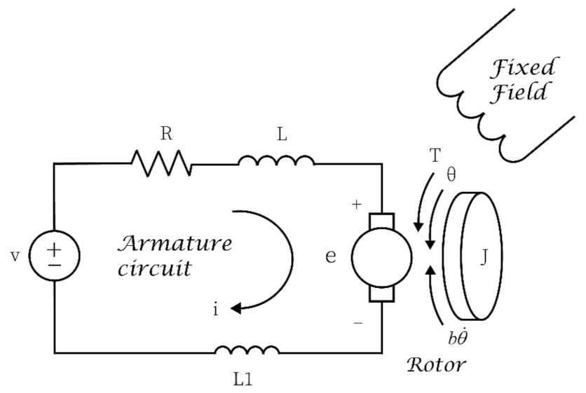
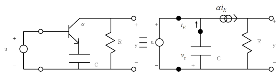
Example 2.

A popular actuator widely used in control systems is DC motor. The DC motor model in [38] is modified and adapted for this example.Figure 1 shows the free-body diagram of the rotor and the equivalent circuit of the armature. As seen in the figure, a small inductor L1 externally connected in series with armature circuit of a DC motor serves as the only sensor of the control system and we assume that tachometer is not installed to measure the rotational speed$\dot{\theta }$of the shaft. The voltage of L1 is measured and used in feedback controller design. Unlike the traditional DC motor controls which apply state related feedback of angular velocity or current, the inductor’s voltage$(\mathrm{L}1\frac{d\mathrm{i}}{dt})$is state derivative related measurement feedback of current derivative which is well suitable to apply the proposed IOC algorithm based on state derivative feedback. Furthermore, inductor’s average power is zero so it does not damage the armature circuit. Therefore, the controller can save implementation cost and avoid power lose.

In this example, torque tracking controller and rotational speed tracking controller are constructed based on the design algorithm of inverse optimal control for affine SDS Systems with state derivative related feedback. This example is used to illustrate the design method in Section 2.3 for linear time invariant SDS systems, namely RSS systems.

From the above figure, according to Newton’s second law and Kirchhoff’s voltage law, we can get the following governing Equations.

$$\mathrm{J}\ddot{\theta }+b\dot{\theta }=K\mathrm{i}$$

$$\left(\mathrm{L}+\mathrm{L}1\right)\frac{d\mathrm{i}}{dt}+\mathrm{i}R=\mathrm{v}-K\dot{\theta }$$

where i is armature circuit’s current, $\theta$ is rotor’s rotational angle, R is electric resistance, L is electric inductance, J is rotor’s moment of inertia, b is motor viscous friction constant, L1 is the external inductor sensor connected in series with armature circuit, and K represents both electromotive force constant and motor torque constant in SI unit.

For simulation purpose, the DC motor’s physical parameters in this example are given as R:$1 \mathsf{\Omega }$, L: $0.49 \mathrm{H}$, J: $0.01 kg.m^2$, L1: $0.01 \mathrm{H}$ and $K:$ $0.01 V/rad/sec$ for electromotive force constant and $0.01 N.m/Amp$ for motor torque constant.

Defining state vector as $x=\left[\begin{array}{c}\dot{\theta }\\ \mathrm{i}\end{array}\right]$, using the governing equations, one can obtain the following SDS system.

$$x=\left[\begin{array}{c}\dot{\theta }\\ \mathrm{i}\end{array}\right]=\frac{1}{\mathrm{R}b+K^2}\left[\begin{array}{cc}-\mathrm{RJ}& -K(\mathrm{L}+\mathrm{L}1)\\ K\mathrm{J}& -(\mathrm{L}+\mathrm{L}1)\end{array}\right]\left[\begin{array}{c}\ddot{\theta }\\ \frac{d\mathrm{i}}{dt}\end{array}\right]+\frac{1}{\mathrm{R}b+K^2}\left[\begin{array}{c}K\\ b\end{array}\right]\mathrm{v}$$

(83)

Substituting the physical parameters of the DC motor into above SDS system, one obtains

$$x=\left[\begin{array}{c}\dot{\theta }\\ \mathrm{i}\end{array}\right]=\left[\begin{array}{cc}-0.0999& -0.05\\ 0.001& -4.995\end{array}\right]\left[\begin{array}{c}\ddot{\theta }\\ \frac{d\mathrm{i}}{dt}\end{array}\right]+\left[\begin{array}{c}0.0999\\ 0.9990\end{array}\right]\mathrm{v}=f\dot{x}+gu$$

(84)

Since the L1 inductor’s voltage is state derivative related measurement, the measurement of the system is given as

$$y=\left[\begin{array}{cc}0& \mathrm{L}1\end{array}\right]\left[\begin{array}{c}\ddot{\theta }\\ \frac{d\mathrm{i}}{dt}\end{array}\right]=\left[\begin{array}{cc}0& 0.01\end{array}\right]\left[\begin{array}{c}\ddot{\theta }\\ \frac{d\mathrm{i}}{dt}\end{array}\right]=C\dot{x}$$

(85)

The measurement feedback control law is given as

$$u=-ky=-kC\dot{x}$$

where k is the measurement feedback gain.

If the rotational speed of the shaft $\dot{\theta }$ needs to track a reference command $r_0$, the performance output equation is given as follows.

$$z=\left[\begin{array}{cc}1& 0\end{array}\right]\left[\begin{array}{c}\dot{\theta }\\ \mathrm{i}\end{array}\right]=H_{s}x$$

(86)

If the torque $T=K\mathrm{i}$ needs to track a reference command $r_0$, the performance output equation is given as follows.

$$z=\left[\begin{array}{cc}0& K\end{array}\right]\left[\begin{array}{c}\dot{\theta }\\ \mathrm{i}\end{array}\right]=\left[\begin{array}{cc}0& 0.01\end{array}\right]\left[\begin{array}{c}\dot{\theta }\\ \mathrm{i}\end{array}\right]=H_{t}x$$

(87)

From (83) to (84), the DC motor model is linear and time invariant. Therefore, the SDS system is also a RSS system as mentioned in introduction section. Therefore, the open loop system poles: −9.9975 and −2.0025 are the reciprocals of the eigenvalues of matrix f in the system. Although the open loop RSS system is stable, its tracking performance can be further improved.

To carry out tracking control, the closed loop system should be stable.

First, a symmetric and positive definite matrix P serving as the design parameter for Lyapunov function $V\left(x\right)$ in (11) is selected as follows.

$$P=\left[\begin{array}{cc}1& 0\\ 0& 0.5\end{array}\right].$$

Followed by selecting another design parameter $R\left(\dot{x}\right)$ as

$$R\left(\dot{x}\right)=0.0004.$$

To ensure the closed loop system is stable, based on (37), the $L_2\left(\dot{x}\right)$ is selected as

$$L_2\left(\dot{x}\right)=\left[\begin{array}{cc}\ddot{\theta }& \frac{d\mathrm{i}}{dt}\end{array}\right]\left[\begin{array}{c}-0.0999\\ -0.4999\end{array}\right].$$

Using (34), the inverse optimal law $\varphi \left(\dot{x}\right)$ is obtained as

$$\varphi \left(\dot{x}\right)=0.497976\frac{d\mathrm{i}}{dt}=-kC\dot{x}=-k\left[\begin{array}{cc}0& 0.01\end{array}\right]\left[\begin{array}{c}\ddot{\theta }\\ \frac{d\mathrm{i}}{dt}\end{array}\right]=-0.01k\frac{d\mathrm{i}}{dt}.$$

Therefore, we obtain the measurement feedback gain k in (85) as

$$k=-49.7976.$$

Consequently, use (38) to obtain $L_1\left(\dot{x}\right)$ as

$$L_1\left(\dot{x}\right)=\left[\begin{array}{cc}\ddot{\theta }& \frac{d\mathrm{i}}{dt}\end{array}\right]\left[\begin{array}{cc}0.0999& 0.0500\\ -0.0005& 0.2498\end{array}\right]\left[\begin{array}{c}\ddot{\theta }\\ \frac{d\mathrm{i}}{dt}\end{array}\right]$$

and use (41) to obtain the performance integrand $L(\dot{x},u)$.

Applying the obtained control law with feedback gain, the close loop system poles have been moved to better locations at −10.0102 and −493.9479. We use the following tracking controller to illustrate the improvement of closed loop system.

$$u=-ky+N{r}_0=-kC\dot{x}+N{r}_0$$

where $r_0$ is given reference command vector to be tracked by performance output and N is a feedforward gain to be designed.

The steady state derivative is zero $\hspace{0.17em}(\dot{\overline{x}}(\infty )=0$) when the RSS closed loop system is stable. In that case, the steady state is

$$\overline{x}=\left(f-gkC\right)\dot{\overline{x}}+gN{r}_0=gN{r}_0.$$

If the performance output is $z=Hx$, to have zero tracking error of steady state, let

$$\overline{\epsilon }(\infty )=r_0-H\overline{x}=r_0-HgN{r}_0=(I-HgN)r_0=0.$$

Consequently, the feedforward gain N is obtained as

$$N={(Hg)}_{right}{}^{-1}$$

(88)

where $(Hg){\hspace{0.17em}}_{right}^{-1}$ is the right inverse of matrix Hg.

If Hg is a full rank matrix with the size of $m\times n$ and $m\le n$, we have

$$(Hg){\hspace{0.17em}}_{right}^{-1}={(Hg)}^T{(Hg{(Hg)}^T)}^{-1}$$

The feedforward gain N and feedback gain k can be designed separately because they are independent of each other.

Therefore, according to (86), for rotational speed tracking, we have feedforward gain $N_s$ as

$$N_s={(H_{s}g)}_{right}{}^{-1}=10.01$$

Similarly, for motor torque tracking, from (87) we have feedforward gain $N_t$ as

$$N_t={(H_{t}g)}_{right}{}^{-1}=100.1$$

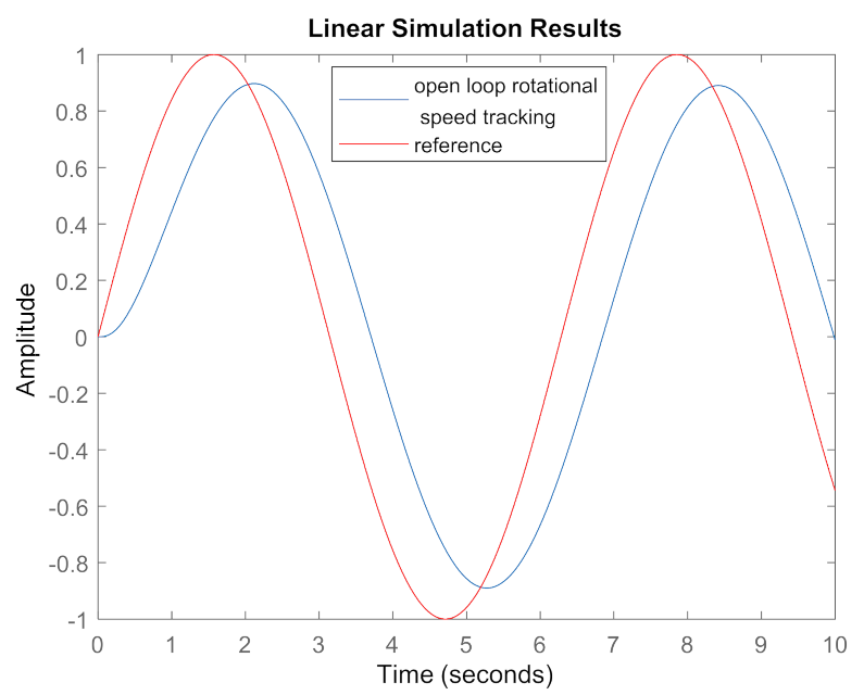
Since the open loop system is stable, we can give the reference command for system to track. As seen in Figure 2, there are obvious attenuation and phase lag for tracking a $\sin t$ reference command of rotational speed $\dot{\theta }$.

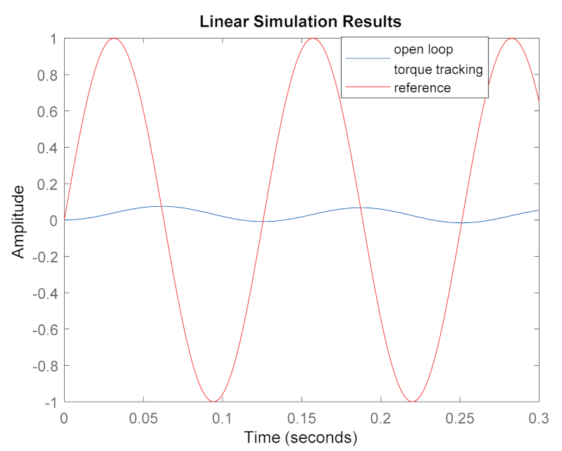
Furthermore, as seen in Figure 3, both attenuation and phase lag are large for tracking a $\sin 50t$ waveform of reference command of torque $K\mathrm{i}$.

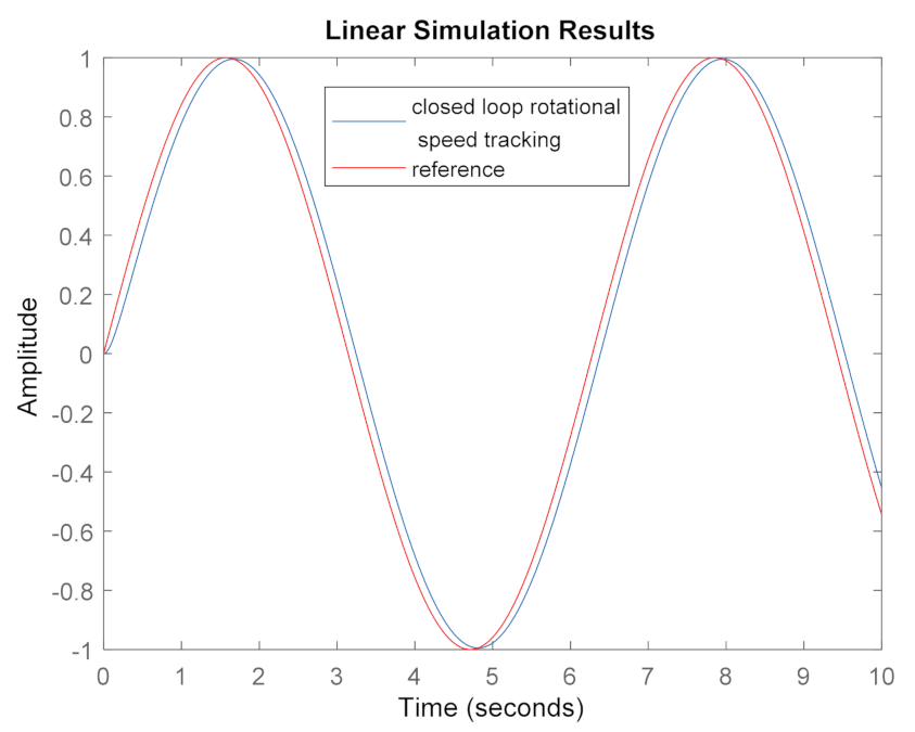
Therefore, tracking performance should be improved. Applying the obtained inverse optimal law, as seen in Figure 4, rotational speed $\dot{\theta }$ can better track $\sin t$ reference command. There is no attenuation and phase lag is only ${5.72}^{°}$.

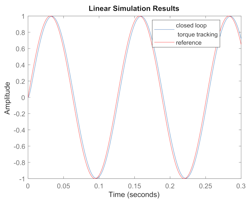
Applying the obtained inverse optimal law, as seen in Figure 5, torque $K\mathrm{i}$ can track $\sin 50t$ reference command much better. There is no attenuation and phase lag is only ${5.72}^{°}$.

Therefore, the control law works well to improve the tracking performance.

Example 3.

The following circuit in Figure 6 is a typical singular system with impulse mode from [39] with C = 1. It is unstable and has pole at infinity. This example is used to illustrate the design approach of Inverse Optimal Control for Affine SDS Systems with $L_2$Disturbance in Section 2.4.

$$E\dot{x}=\left[\begin{array}{cc}1& 0\\ 0& 0\end{array}\right]\dot{x}=\left[\begin{array}{cc}0& 1\\ 1& 0\end{array}\right]x+\left[\begin{array}{c}0\\ 1\end{array}\right]u=Fx+Nu, x=\left[\begin{array}{c}{v}_c\\ i_E\end{array}\right]=\left[\begin{array}{c}{x}_1\\ x_2\end{array}\right]$$

Since matrix F is invertible, the singular system with impulse mode can be expressed in the following SDS system form.

$$x=F^{-1}E\dot{x}-F^{-1}Nu=f\dot{x}+gu$$

(89)

For verifying the proposed algorithm, external disturbance $\omega$ is added to the system as follows.

$$\begin{gathered} x=\left[\begin{array}{cc}0& 0\\ 2& 0\end{array}\right]\dot{x}+\left[\begin{array}{c}-1\\ 0\end{array}\right]u+\left[\begin{array}{c}0.1\\ -0.1\end{array}\right]\omega =f\dot{x}+gu+J_1\omega \\ z=\left[\begin{array}{cc}2& 1\end{array}\right]\dot{x}+0.8u=h\dot{x}+Ju \\ u=-K_{\infty }\dot{x}, \gamma =0.6 \end{gathered}$$

First, a symmetric and positive definite matrix P serving as the design parameter for Lyapunov function $V\left(x\right)$ in (11) is selected as follows.

$$P=\left[\begin{array}{cc}1& 0\\ 0& 1\end{array}\right].$$

Followed by selecting another design parameter $R\left(\dot{x}\right)$ as

$$R\left(\dot{x}\right)=1.$$

Consequently,

$$\mathsf{\Gamma }\left(\dot{x},u\right)={\dot{x}}^T\left[\begin{array}{cc}4.0069& 1.9931\\ 1.9931& 1.0069\end{array}\right]\dot{x}+{\dot{x}}^T\left[\begin{array}{c}3.2\\ 1.6\end{array}\right]u+0.64u^{T}u$$

To ensure the closed loop system is stable, based on (64), the $L_2\left(\dot{x}\right)$ is selected as

$$L_2\left(\dot{x}\right)=\left[\begin{array}{cc}{\dot{x}}_1& {\dot{x}}_2\end{array}\right]\left[\begin{array}{c}-9.9759\\ -4.9702\end{array}\right]$$

(90)

Then using (62) yields

$$\varphi \left(\dot{x}\right)=\left[\begin{array}{cc}2.3707& 1.0275\end{array}\right]\dot{x}=-K_{\infty }\dot{x}$$

(91)

Therefore, the obtained full state derivative feedback gain is

$$K_{\infty }=\left[\begin{array}{cc}-2.3707& -1.0275\end{array}\right].$$

Applying the control law, the closed loop system poles locate at $-0.5768 \pm 0.3923\mathrm{i}$. Since their real parts are all negative, the closed loop system are stable.

Applying (65), we have

$$L_1\left(\dot{x}\right)={\dot{x}}^T\left[\begin{array}{cc}2.2102& 2.0018\\ 0.0018& 0.7245\end{array}\right]\dot{x}$$

Furthermore, applying (91) obtains

$$\mathsf{\Gamma }\left(\dot{x},\varphi \left(\dot{x}\right)\right)={\dot{x}}^T\left[\begin{array}{cc}15.1901& 7.0926\\ 7.0926& 3.3266\end{array}\right]\dot{x}$$

(92)

Substituting (90) and (92) into (64) yields

$$-12.5019x^{T}x<0$$

It proved that $L_2\left(\dot{x}\right)$ is properly selected.

In addition, this SDS system is actually controllable with state derivative feedback control. For example, if we want to assign the closed loop poles at −2 and −4 using full state derivative feedback control law $u=-K\dot{x}$, the closed loop SDS system becomes

$$x=f\dot{x}+gu=(f-gK)\dot{x}.$$

The gain K should be designed such that matrix $\left(f-gK\right)$ has eigenvalues at −0.5 and −0.25 because they are the reciprocals of −2 and −4, respectively. In this case, using Matlab command place, one can easily find $K=\left[\begin{array}{cc}-0.7500& -0.0625\end{array}\right]$. Therefore, using state derivative feedback control, it is possible to assign all closed loop poles for some singular systems with impulse mode if they can be expressed in a controllable SDS system form. However, using state feedback control, it is impossible to assign all closed loop poles for any singular systems. It is only possible to stabilize some of the singular systems with state feedback control.

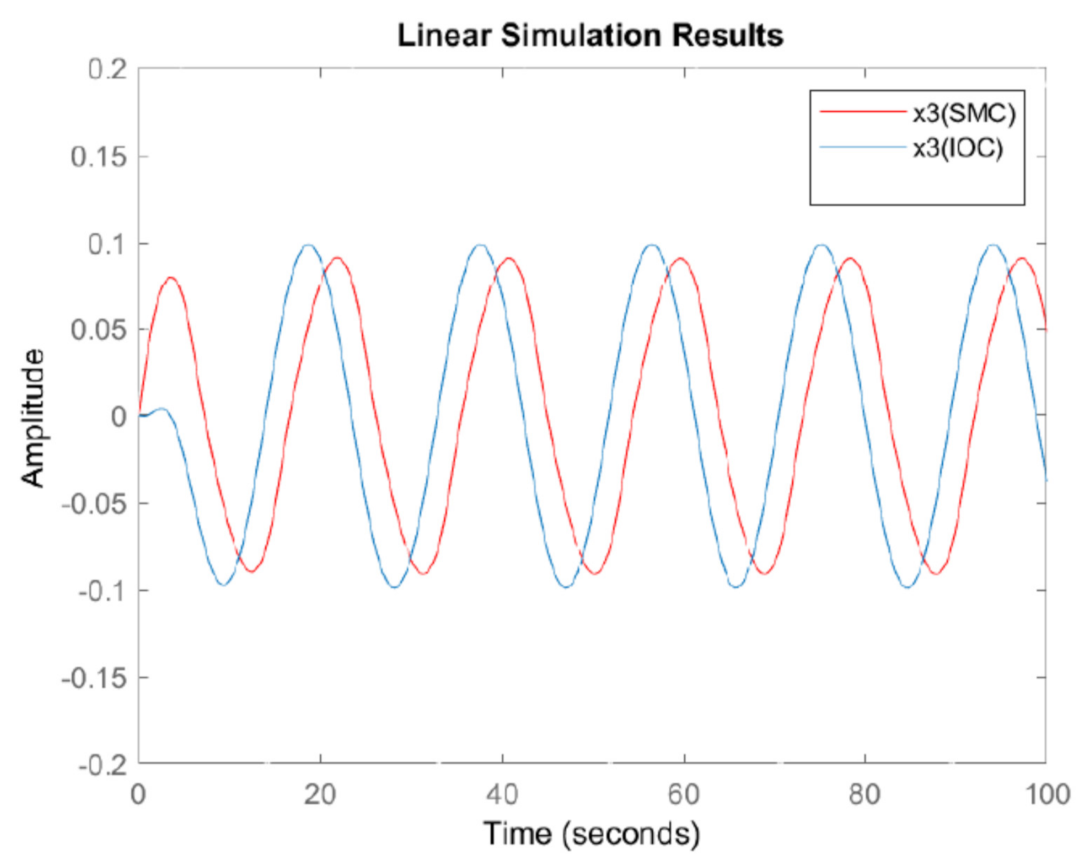
Example 4.

It is interesting to compare the proposed inverse optimal control (IOC) in Section 2.4 with sliding mode control (SMC) design for SDS system with matched disturbance because they are both developed based on Lyapunov stability theorem. Consider the following unstable SDS system with matched disturbance given in [20].

$$x(t)=f\dot{x}(t)+gu(t)+J_1\omega (t)=f\dot{x}+g(u+\omega (t)), t\ge 0$$

(93)

where $f=\left[\begin{array}{ccc}1& -0.5& 0.25\\ 0& 0.5& -0.25\\ 0& 0& 0.5\end{array}\right]$, $g=J_1=\left[\begin{array}{c}-0.25\\ 0.25\\ -0.5\end{array}\right]$ (for matched disturbance), $x(t)=\left[\begin{array}{c}\mathrm{x}1\\ \mathrm{x}2\\ \mathrm{x}3\end{array}\right]$, and $\omega (t)=0.2\sin 0.3333t$, with the following full state derivative performance variables.

$$z=h\dot{x}\left(t\right)+Ju\left(t\right)=\dot{x}\left(t\right)$$

where $h=I_{3\times 3}$ (identity matrix) and $J={[0 0 0]}^{\mathrm{T}}$.

(a)

For sliding mode control (SMC) [20], the sliding surface is selected as

$$s=\left[\begin{array}{ccc}-84& -180& -50\end{array}\right]x=Cx$$

Consequently, we have $Cg=1$.

The ideal controller is given as

$$u\left(t\right):=-{(Cg)}^{-1}Cf\dot{x}\left(t\right)-{(Cg)}^{-1}(\gamma +\alpha )sign\left(\dot{s}\left(t\right)\right)$$

(94)

where $\Vert \gamma \Vert >\Vert Cg\omega \left(t\right)\Vert =0.2$ in this example for countermeasure the matched disturbance and $\alpha >0$ should be selected to ensure that the approaching condition can happen.

In [20], it has been proven that applying the ideal controller in (94), the following approaching condition happens.

$$s^T\left(t\right)\cdot \dot{s}\left(t\right)<-\alpha \cdot \Vert \dot{s}\left(t\right)\Vert <0$$

To avoid or reduce “chattering phenomenon” due to $sign\left(\dot{s}\left(t\right)\right)$ switching function in (94), the following modified controller is used.

$$u\left(t\right):=-{(Cg)}^{-1}Cf\dot{x}\left(t\right)-{(Cg)}^{-1}(\gamma +\alpha )sat\left(\dot{s}\left(t\right),\epsilon \right)$$

(95)

where ″sat″ is a saturation function to smoothly handle the switching as follows.

$$sat(\dot{s},\epsilon )=\{\begin{array}{cc}1& \dot{s}>\epsilon \\ \frac{\dot{s}}{\epsilon }& \left|\dot{s}\right|\le \epsilon \\ -1& \dot{s}<-\epsilon \end{array}=\{\begin{array}{cc}sign\left(\dot{s}\right)& \left|\dot{s}\right|>\epsilon \\ \frac{\dot{s}}{\epsilon }& \left|\dot{s}\right|\le \epsilon \end{array}$$

Here $\epsilon$ is a small positive value as the bound of the differential sliding surface $\dot{s}$ such that

$$\left|\dot{s}\right|\le \epsilon$$

In this example $\epsilon =0.5$,$\gamma =0.4$ and $\alpha =0.05$ are used in the simulation. When sliding surface is selected, we need to tune design parameters of $\epsilon$, $\gamma$ and $\alpha$ to have a SMC controller with good enough performance.

(b)

For applying the inverse optimal control (IOC) design method in Section 2.4, we can follow the same design steps and use the same notations in example 3. In this example, we have

$$h=I_{3\times 3} (\mathrm{identity} \mathrm{matrix}) \mathrm{and} J={[0 0 0]}^{\mathrm{T}}$$

First, we select the following design parameters as

$$\gamma =0.6, P=I_{3\times 3} (\mathrm{identity} \mathrm{matrix}) \mathrm{and}R\left(\dot{x}\right)=1$$

To ensure the closed loop system is stable, based on (64), the $L_2\left(\dot{x}\right)$ is then selected as

$$L_2\left(\dot{x}\right)=\left[\begin{array}{cc}\dot{\mathrm{x}}1& \begin{array}{cc}\dot{\mathrm{x}}2& \dot{\mathrm{x}}3\end{array}\end{array}\right]\left[\begin{array}{c}-79.75\\ -76.25\\ -17.50\end{array}\right]$$

Consequently, using (62) yields

$$\varphi \left(\dot{x}\right)=\left[\begin{array}{ccc}40.00& 38.00& 9.00\end{array}\right]\dot{x}=-K_{\infty }\dot{x}$$

Therefore, the obtained full state derivative feedback gain is

$$K_{\infty }=\left[\begin{array}{ccc}-40.00& -38.00& -9.00\end{array}\right].$$

Applying this control law, the closed loop system poles locate at $-0.5 \pm 0.5\mathrm{i}$ and $-1$. Since their real parts are all negative, the closed loop system are stable.

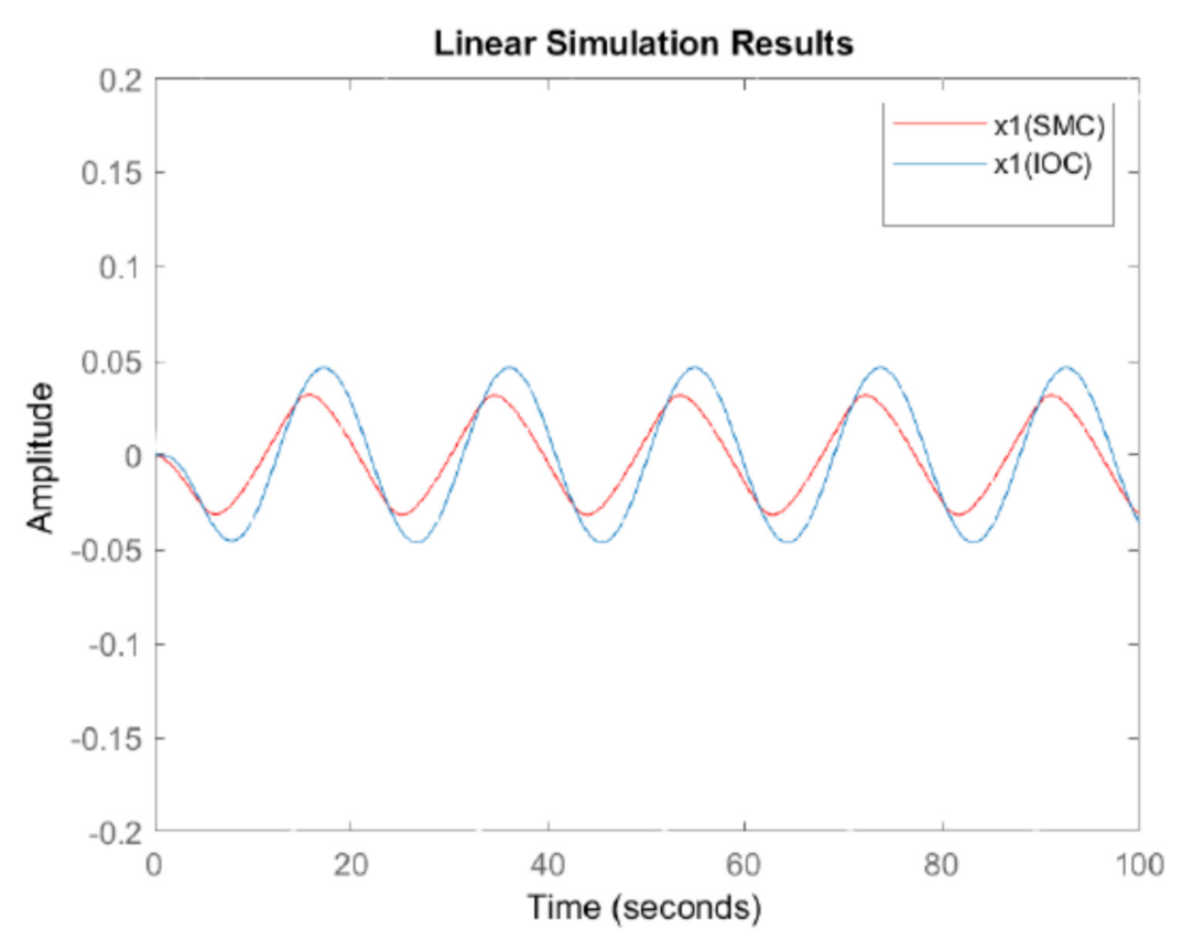
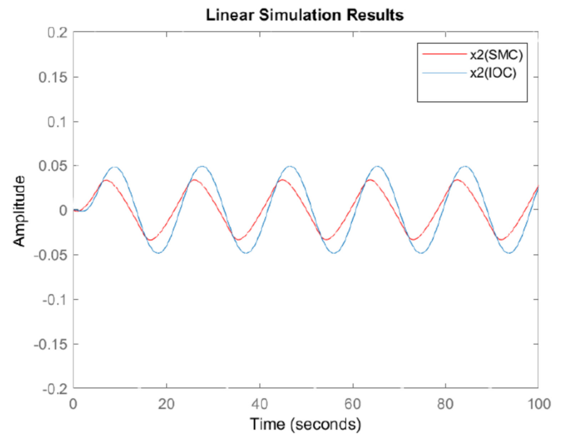
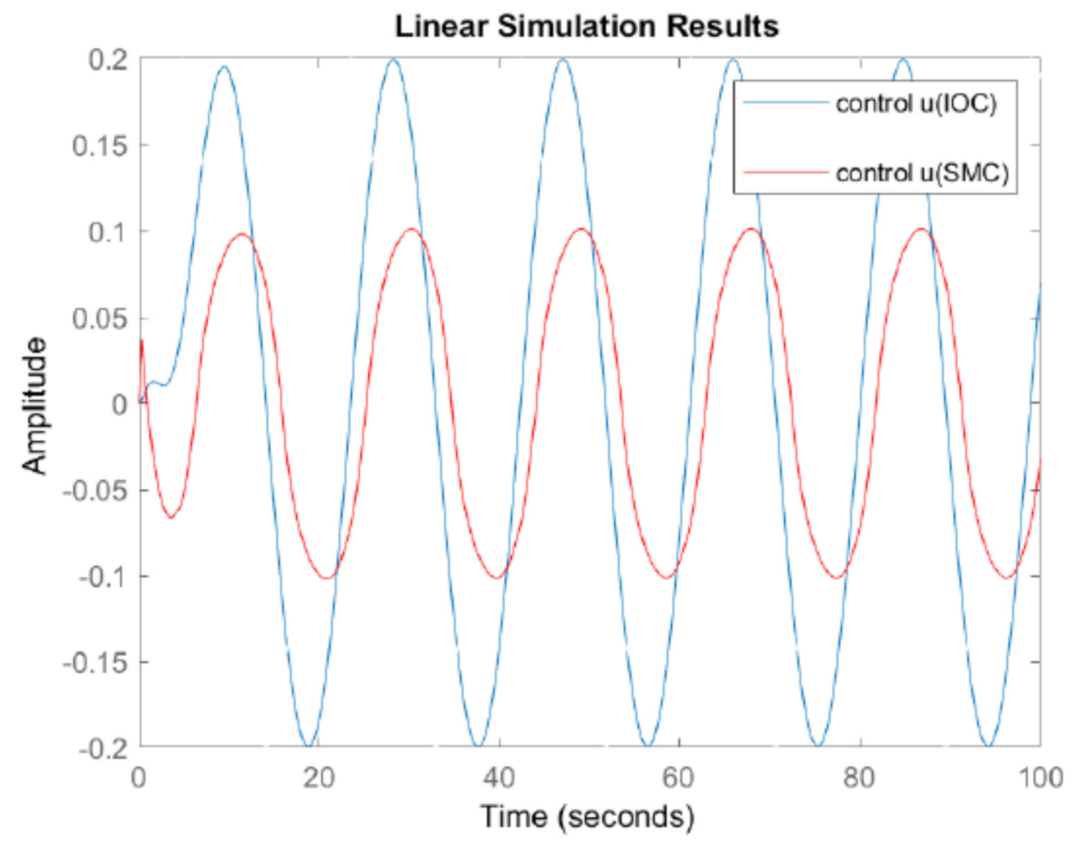
The state responses and control effort of both SMC and IOC are plotted in the following figures for comparisons.

The unstable system in this example can be properly controlled by both sliding mode control (SMC) and inverse optimal control (IOC) to have bounded closed loop state responses. As shown in Figure 7, Figure 8, Figure 9 and Figure 10, for matched disturbance case in this example, when SMC is properly designed, its performance could be better than that of IOC because SMC can have smaller state responses in Figure 7, Figure 8 and Figure 9 by applying smaller control effort in Figure 10.

4. Discussion

The proposed design methods are inspired by other previous work [26,27,31] in inverse optimal control in state space system with state feedback design approach. The results show that the use of state derivative feedback for control design in an SDS system is as simple as the use of state feedback for control design in a state space system.

Therefore, with the understanding of SDS systems, many design tools developed in state space system with state feedback can be modified and adapted for control designs in SDS system with state derivative feedback. Since the Hamilton–Jacobi–Bellman equation is not always solvable to obtain the control Lyapunov function, the existence of optimal control solution is not always guaranteed. On the other hand, if we can solve for a control Lyapunov function from HJB equation, we can find from it a control law that achieves the minimum of performance functional and the resulting closed loop system has a unique solution forward in time. Please refer to Chapter 6 in [27] for details, the descriptions and formula derivations are analogous to those for SDS system case. Since the control Lyapunov function is predefined in inverse optimal control design process and no need to solve HJB equation, it is very suitable to find stabilizing control laws for unstable nonlinear systems.

Regarding the examples to verify the proposed methods, Example 1 demonstrates the design steps for the design approach of inverse optimal control for affine SDS systems with state derivative related feedback. In the same example, it also suggests that people should free their mindset in control designs. No matter the system in state space form or SDS form, the possibilities of applying state feedback or state derivative feedback should be both checked so that the controller can be simple while perform well. The DC motor tracking control without tachometer in Example 2 discusses the possibility of using alternative measurement of inductor voltage in DC motor control based on the obtained state derivative feedback algorithms. This idea seems promising, because the method we propose can construct a cheap and compact controller without the need for an expensive tachometer. Furthermore, unlike resistor sensor, the average power of inductor sensor is zero, it will not damage the armature circuit or cause power loss. Example 3 is a singular system with impulse mode. This is a very challenging design problem in previous researches using state feedback in control design of the generalized state space system. Since it can be expressed in SDS system, the design approach is straightforward. Therefore, some systems that are difficult to control through state feedback can be controlled through state derivative feedback in SDS system form.

Since both sliding mode control (SMC) [19,20] and the inverse optimal control in SDS system form are developed based on Lyapunov stability theorem and their performances are dependent on tuning their design parameters, we compare them in terms of conditions to use and limitations. SMC methods in [19,20] have low sensitivity to parameter uncertainties, can work with matched uncertainties as well as matched disturbance that enter into control inputs and apply discontinuous switching control law to ensure the finite time convergence. Those are their advantages. However, SMC methods in [19,20] may suffer from chattering phenomenon and when uncertainties and disturbance are not matched ones, the performance could be downgraded. On the contrary, the inverse optimal control method in Section 2.4 can handle bounded disturbance which are not from control inputs. As shown in Example 4, for system with matched disturbance, the SMC controller could use smaller control effort to obtain smaller state responses than IOC controller. However, from the implementation point of view, the structure of IOC controller is simpler than that of SMC controller and consequently the implementation cost of IOC controller could be cheaper. The inverse optimal control methods in this paper are suitable for controlling the system with precise parameters, such as the DC motor used for tracking control in Example 2. Therefore, designers can make tradeoff between IOC and SMC in terms of performance and cost.

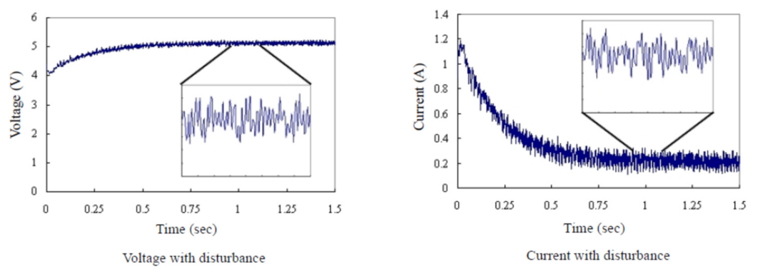
Regarding the future works, for implementation of the DC motor application in example 2, as seen in Figure 1, there is large electric inductance L in armature circuit in the model of DC motor. No matter what kind of sensor we use, one potential problem that is common in DC motor control is inductive kick (kickback) phenomenon or so called Ldi/dt voltages [39]. Since the windings of the DC motor will produce current conversion during commutation, the current conversion will cause the inductive kickback that disturbs both the voltage and current of armature circuit as shown in Figure 11. Therefore the measured voltage of L1 sensor in Figure 1 will also be disturbed.

Conventionally, in implementation, various absorption circuits of inductive load kickback [40] can be used as the countermeasure for disturbance caused by inductive kick. Other than applying absorption circuits, we are considering another solution of eliminating disturbance of L1 sensor voltage due to inductive kick in our future research. The basic idea is as follows. Since the inductive kick is formed by periodic commutation, it has an average of 0 characteristics, if the T is the time of every commutator segment passes through a brush, selecting the signal window of L1 sensor voltage with a period as a multiple of T and calculating the average voltage value of window, the L1 voltage disturbance caused by the inductive kick of commutators could be considerably decreased. The control voltage is then generated by feedback of L1 voltage with reduced disturbance. In addition, since this disturbance of L1 sensor voltage is through control input channel, it can be considered as matched disturbance. Hence, we will also consider to apply sliding mode control with state derivative measurement feedback to control it in future.

In this paper, we have proven that the inverse optimal control can be carried out in SDS system form with state derivative feedback. In future, more challenging problems such as stochastic systems can be explored. If a system has randomness associated with it, it is called a stochastic system and does not always produce the same output for a given input. Stochastic systems exist in many applications such as communication systems, markets, social systems, and epidemiology. Optimal control [41,42] and inverse optimal control [42,43] for stochastic systems in state space system form have been solved with stochastic Hamilton–Jacobi–Bellman equation to obtain state related feedback control laws. In future, for people who want to develop inverse optimal control for stochastic systems with state derivative feedback, it is highly recommended to first study [42] because the design approaches in [42] and this paper are both built on [27].

5. Conclusions

In this paper we have discussed about how SDS system with state derivative feedback can be supplement of state space system with state feedback in control designs. Followed by developing inverse optimal control methods in SDS systems with solely state derivative feedback. As far as the authors know, no similar results have been reported. Inverse optimal control can construct a stable closed-loop system while nonlinear optimal control may not have exact solution. Hence, inverse optimal control should be collaboratively used together with optimal control for designs. The proposed methods are very suitable to find stabilizing control laws for unstable nonlinear systems. The correctness of proposed methods has been properly verified by numerical examples and simulations. Especially, in the third example, a classic difficult problem in control, namely singular system with impulse mode is fully controllable by state derivative feedback in SDS system form and satisfy the non-expansivity constraint when the system is subjected to disturbance. On the contrary, the same system can only be stabilized by state feedback control. The above is the summary of academic contributions of this paper.

From application points of view, in vibration systems of vehicle dynamics and smart structure, accelerations and velocities are available measurements of state derivative vector. In addition, the inductor voltages in electrical systems are also state derivative related measurement. For those systems, using state derivative feedback design in SDS system form are very likely to have more simple, cheap and compact controllers because integrators or numerical integrations are not needed. Therefore, the idea of connecting a small inductor in series with an armature circuit as the only sensor of a DC motor control system in Example 3 is very promising because average power loss of inductor is zero and no tachometer is needed. DC motors are widely used in many industries and facilities for daily life. For example, in automotive body electronics, the estimated demand for automotive DC motors in body domain was 2 billion units in 2020 [44]. So the proposed design approach of this paper can have a wide range of practical applications.

With understandings and awareness of SDS system form, state derivative feedback and inverse optimal control, designers can solve more control problems and develop more new applications based on their previous knowledge and experience in state feedback designs in state space system without applying too much of advanced mathematics.

6. Patents

Authors, Yuan-Wei Tseng and Rong-Ching Wu hold the following patents related to state derivative feedback control in SDS systems.

• US Patent NO. US 10,598,688 B2, “Oscillation Control System and Oscillation Control Method”, 2020.03.24~2038.09.20
  (https://patents.google.com/patent/US10598688B2/en?oq=US+10%2c598%2c688+B2) (accessed on 16 March 2021).
• Taiwan Patent NO. I670924, “Vibrational Control System”, 2019.09.01~2038.07.01