Noninvasive Detection of Appliance Utilization Patterns in Residential Electricity Demand ^†

Abstract

Smart meters with automatic meter reading functionalities are becoming popular across the world. As a result, load measurements at various sampling frequencies are now available. Several methods have been proposed to infer device usage characteristics from household load measurements. However, many techniques are based on highly intensive computations that incur heavy computational costs; moreover, they often rely on private household information. In this paper, we propose a technique for the detection of appliance utilization patterns using low-computational-cost algorithms that do not require any information about households. Appliance utilization patterns are identified only from the system status behavior, represented by large system status datasets, by using dimensionality reduction and clustering algorithms. Principal component analysis, k-means, and the elbow method are used to define the clusters, and the minimum spanning tree is used to visualize the results that show the appearance of utilization patterns. Self organizing maps are used to create a system status classifier. We applied our techniques to two public datasets from two different countries, the United Kingdom (UK-DALE) and the US (REDD), with different usage patterns. The proposed clustering techniques enable effective demand-side management, while the system status classifier can detect appliance malfunctions only through system status analyses.

1. Introduction

The use of residential appliances is directly affected by the daily and weekly routines of people who live in the house. School and work schedules, eating habits, laundry, and other personal preferences or schedules affect the electricity demand in different households. Currently, with the social distancing imposed in most countries because of the COVID-19 pandemic, many of these patterns have changed; see, for instance, [1]. New appliances, remote work, and lockdowns have led to more people staying at home and thus have changed individual and aggregate daily consumption profiles. In general, personal routines are not easy to change, especially when it refers to what people do inside their homes; thus, automated solutions might be beneficial to manage the electric load demand [2,3]. From this perspective, it is clear that studying patterns of consumption is very important at present.

With the recent advances in disaggregation algorithms and the Internet of Things (IoT) [4], the system status can be obtained in a nonintrusive way, with only the information of the total power demand recorded by the smart meter. Feedback on the system status behavior could be offered either by the energy supplier itself or by a consultant company, always with the consent of the customer. By the detailed detection of the utilization patterns [5,6], it is possible to gain a better understanding of consumers’ habits and provide feedback, such as individual contracts, using real-time mobile applications with suggestions to improve the energy efficiency of the residence. This can be a motivating factor for more people to agree on having their residence monitored. In this context, several studies have already been performed on the demand side with the aim to characterize and classify the consumers in order to improve the energy efficiency [7,8,9,10]. In [11], for example, eighteen characteristics of the household and its occupants have been inferred from aggregated power measurements, with accuracy levels reaching over 80%. All these studies were conducted using intrusive monitoring to determine the system status, but, most importantly, by using other information about the house occupants and appliance characteristics to derive conclusions. This work describes a technique for the detection of utilization patterns using low-computational-cost algorithms, but unlike other works already published no further information about the appliances or occupants of the house is used.

With the large storage capacity available in clouds and several load monitoring programs [11,12,13], several data sets are now available with real house samplings and with a high quality of information, such as sampling periods from minutes to seconds, different harmonic ranges and monitoring periods, and other interesting characteristics. Some of the public data sets contain the model and manufacturer of the appliances, for example. Moreover, with the advancements in Information and Communication Technologies (ICTs), it has become feasible to process such a large amount of data [4,14,15,16].

The present work follows these lines and focuses on the detection of the utilization patterns of different appliances by using two strategies in steps: first, by using only linear and nonparametric algorithms (PCA, k-means clustering, and Minimum Spanning Tree methods) [17,18], the existence of appliance clusters is investigated, and a methodology for defining the groups of appliances inside each group is established. Second, by using nonlinear methods, specifically Self Organizing Maps (SOM), the possibility of using a trained map as a status classifier is explored.

In specific terms, we start from a relatively large set of system states (the larger, the better) and use an established dimensionality reduction method, followed by clustering algorithms, to find utilization patterns. These patterns are represented by groups of appliances that are statistically related (meaning that they are used at the same time). The appliances inside each group do not necessarily have to be used in combination (e.g., video game and TV); rather, they are statistically related, indicating that they are frequently used at the same time.

Our motivation for studying the loads usage patterns comes from industrial or commercial buildings where the process management system reads the system status and commands it (turning on or off devices such as pumps, lights, and cooling system), as indicated in [19,20,21], but with the aim to extend it to households in a non-intrusive manner.

It is important to note that the formulations chosen are well-established; require a small quantity of parameters (in the first step, no parameters at all); and are not related to the household habits, professions, or other personal information of the occupants. In summary, our main contributions are:

• We propose a methodology for the detection of utilization patterns in residential installations with a low computational cost;
• Our method is noninvasive because it does not require any personal information about the households;
• We show that the method for training Self Organizing Maps opens a wide range of analysis opportunities for the system status, starting from malfunction and fault detection.

The paper is organized as follows: Section 1 introduces the work and states the main contributions of the study. Section 2 describes the selected data sets (UK-DALE [13] and REDD [12]), and the formulations that comprise each step of the work (Principal Component Analysis, k-means, Minimum Spanning Tree, Self Organizing Maps). Section 3 provides the results from each step, which are then discussed in Section 4. Finally, Section 5 presents some conclusions and indicates the next steps.

2. Materials and Methods

2.1. Public Dataset Selected

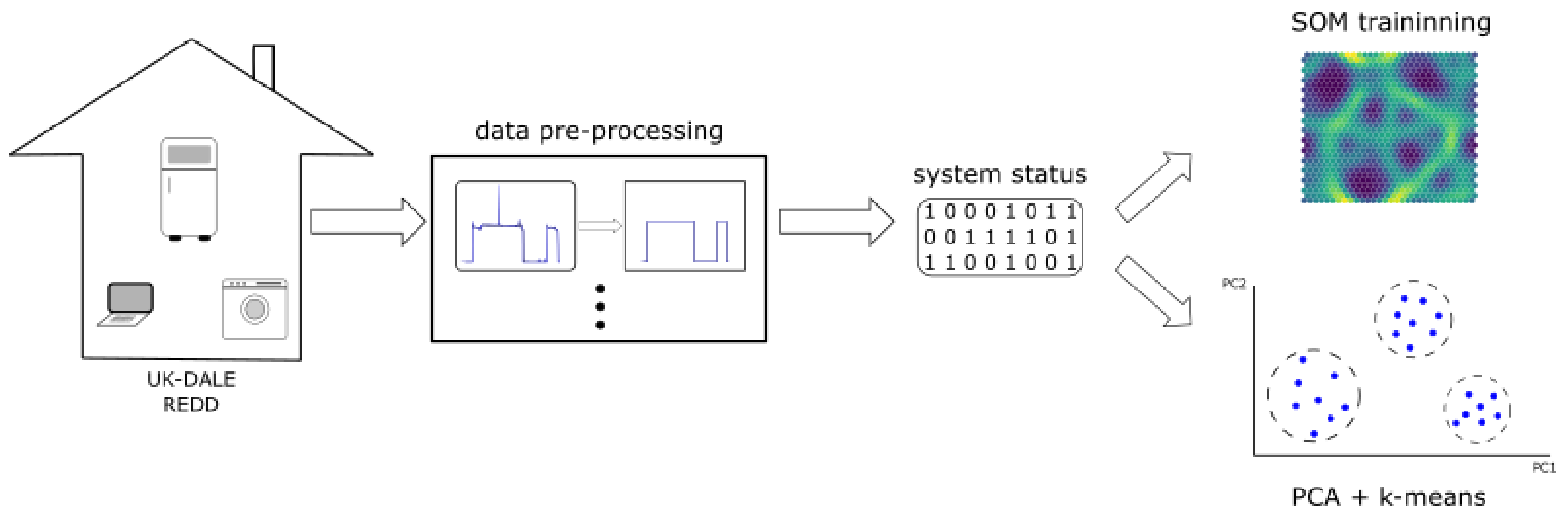
The datasets selected for this study are the UK-DALE [13] and the REDD [12] datasets. The UK-DALE dataset contains measurements from five different households in the United Kingdom with 6-second granularity for periods of more than a month. The measurements contain the individual consumption of 52, 18, 4, 5, and 24 individual channels (each channel can be a single appliance or a group of them); refer to

Table 1. Number of individual channels and time monitored for every house in the UK-DALEdata set.

House	Individual Channels	Time Monitored
UK-DALE HOUSE 1	52	more than 4 years
UK-DALE HOUSE 2	18	193 days
UK-DALE HOUSE 3	4	35 days
UK-DALE HOUSE 4	5	151 days
UK-DALE HOUSE 5	24	122 days
REDD HOUSE 1	18	25 days
REDD HOUSE 2	9	11 days
REDD HOUSE 3	20	14 days
REDD HOUSE 4	18	19 days
REDD HOUSE 5	24	2.7 days
REDD HOUSE 6	15	13 days

for more details.

REDD (Reference Energy Disaggregation Data Set) and UK-DALE (UK Domestic Appliance-Level Electricity) datasets were selected due to their consistency and low granularity, which enable the appliance status to be captured with a high degree of precision. Details about the impacts of the time granularity in electricity metering can be found in [22,23,24]. However, as we are going to discuss later, the proposed analysis is also valid for other time granularities; the only necessary condition is the time synchronization of the time series.

The REDD dataset contains measurements from six different households in the United States with a 3-s granularity, with monitoring periods from 2.7 to 25 days. The monitoring periods are not the best for detecting utilization patterns (unfortunately, 2.7 days can include some holidays, for example, and even 25 days do not cover different seasons of the year), but on the other hand this dataset records a good quantity of individual channels (18, 9, 20, 18, 24, 15), each of them representing one individual appliance.

The information in Table 1 leads to a system state domain of high dimension: ${\mathbb{R}}^{52}$, ${\mathbb{R}}^{18}$, ${\mathbb{R}}^4$, ${\mathbb{R}}^5$, and ${\mathbb{R}}^{24}$ and ${\mathbb{R}}^{18}$, ${\mathbb{R}}^9$, ${\mathbb{R}}^{20}$, ${\mathbb{R}}^{24}$, and ${\mathbb{R}}^{15}$, respectively, for the UK-DALE and the REDD datasets. Considering one sample every 6 s for the UK-DALE dataset, the set of system statuses in one month has more than 400,000 measurements. For the REDD dataset, with one sample every 3 s, the set of system statuses has 28,800 measurements for each monitored day. In addition, if each system status is represented by a binary vector that indicates the status of each appliance (i.e., on or off, or 1 or 0), the number of possible statuses for each house is $2^{52}$, $2^{18}$, $2^4$, $2^5$, and $2^{24}$ for the UK-DALE and $2^{18}$, $2^9$, $2^{20}$, $2^{24}$, and $2^{15}$ for the REDD dataset. These numbers render traditional statistical analysis limited. To address this problem, performing dimensionality reduction is a key step to make the problem more tractable to extract information. Once the system status is in ${\mathbb{R}}^2$ or ${\mathbb{R}}^3$, the distances between the points (appliances) become visible in a chart, and a clustering step (linear with k-means and nonlinear with Self Organizing Maps (SOM)) will define the groups of appliances whose use is related to each other.

2.2. Methodology

To perform the dimensionality reduction using linear transformations, the method of Principal Component Analysis (PCA) [25] was chosen. To perform the same task in a nonlinear approach, the method of Self Organizing Maps (SOM) was used [26].

The preprocessing step was responsible for transforming the demand samples in kW and the corresponding time stamp of each individual channel into a binary vector representing the status of each appliance. The preprocessing includes the following steps:

• The synchronization of the individual channels by removing periods of sampling failure and adjusting small discrepancies between the time stamps of individual channels (some channels were 1 s ahead during some periods, for example);
• The removal of individual channels that contain a quantity of samples too different from the others in the household (the channels with a sample quantity of less than 25% of the average for the installation were removed);
• Definition of the real-power consumption threshold that defines the appliance status as on/1 or off/0; finally,
• The recording the system status set as binary vectors in a text file.

Figure 1 and Figure 2 show the correspondence between the kW sampling of two individual channels and their binary statuses.

The time stamp and the total power in kW are still present in the output file generated by the preprocessing algorithm (see Figure 3 for an example), but as will be explained better later, this information is irrelevant to the results of both PCA and SOM (neither of the methods requires the samples to be consecutive).

The definition of each appliance status is simply based on a real power threshold value. For consumption below this value, the status is “off”, and for the opposite case it is “on”. The possibility of improving the recognition algorithm by using disaggregation techniques, such as appliance signatures (transients during switch on and off) and machine cycles, is known [8,9], but here the focus is on the dimensionality reduction and clustering. Figure 4 shows the proposed approach with its main steps.

Note that the methodology proposed in this paper was developed utilizing disaggregated data. If plugs are directly used for obtaining this data, then the method is clearly intrusive and it is unfeasible to become a scalable solution. However, we anticipate that in more realistic scenarios, an additional block will be included for data disaggregation, which accurately maps the utilization of the appliances (e.g., [27]). It is also worth mentioning that the proposed methodology does work with different time granularities, considering that it allows for detecting the activity of the different appliances. For this, their individual time series must be synchronized to be able to find the patterns of joint usage.

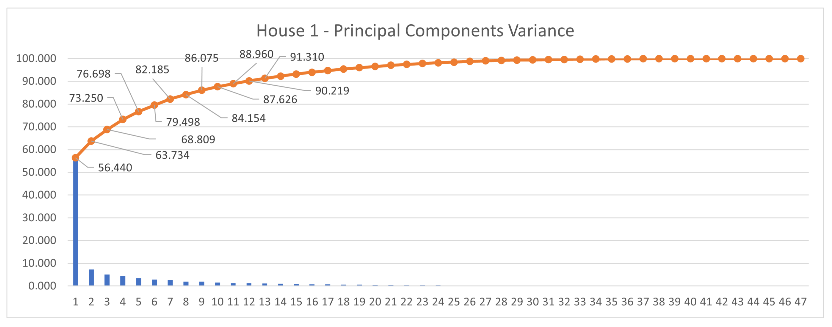
2.2.1. Principal Component Analysis

Principal Component Analysis (PCA) is a linear and nonparametric method that projects high-dimension data into specific directions that lead to variance maximization and noise and redundancy minimization. Refer to [25] for further details.

PCA is an established and simple method for extracting relevant data from noisy or confusing data sets (which can be large or not). In this work, the main advantage of using PCA is that as a result of its capacity of resume redundancy (i.e., with the sampling frequency considered, it is expected that each appliance remains in the same status for several samples), the pattern detection algorithm is simple, linear, and fast. The main advantages of PCA are:

• The method does not require any parametrization, meaning that no additional information of the phenomenon is required.
• The method requires little computational effort.
• The variances associated with each projection direction $p_i$ can be interpreted as a measure of “how principal the component is”; the method lists the components ordered from the largest variance to the lowest.
• As the method is nonparametrical, it is impossible to set it in a wrong way and miss an important result.
• The method does not show any hidden information or suggest any conclusions; instead, it reduces redundancy and shows the data from an angle where the information is easier to visualize.

PCA is especially applicable to our case because we are not looking for any specific cluster; we are only looking for a way of visualizing the system status set in a 2D or 3D projection, thereby making it possible to analyze the data in a simple plot.

The right quantity of principal components necessary to represent the phenomena without significant loss of information is not the same from one problem to another, but it is always related to the total variance accumulated from the PCs [17]. One way to choose how many PCs are enough to represent the data set is to plot the total variance accumulated for every set of PCs. The method, called “the elbow method” [17], applied to this perspective, states that the point where the curve has its elbow (if it has one) is the ideal number of PCs that represent the data set without significant loss of information (variance). If, for example, the curve has no elbow, this means that all the PCs are equally important and PCA is not a good tool to perform dimensionality reduction.

Figure 5 shows a variance curve for the UK DALE data set, House 2. It is clear that from the 6th PC on that the PCs have an insignificant contribution to the variance of the data set. This means that the information they carry, if ignored, has only a small impact on the information captured.

If the first three PCs together add a high percentage of total variance and the total variance curve shows one inflection point at the 3rd PC, this means that the 3D projection of the original data is enough for capturing the data behavior.

For more details about the method and its mathematical formulation, the reader is referred to [17].

2.2.2. Applying PCA to the UK-DALE and REDD Data Sets

The application of PCA to perform the dimensionality reduction in our problem is explained in the following section.

The UK-DALE dataset [13] is composed of five measurement sets of houses in the United Kingdom with 52, 18, 4, 5, and 24 individual channels. The data are collected at every 6 s for a period of more than 4 years, 193 days, 35 days, 151 days, and 122 days, respectively. At each measured instant, the system status is a point in ${\mathbb{R}}^{52}$, ${\mathbb{R}}^{18}$, ${\mathbb{R}}^4$, ${\mathbb{R}}^5$, and ${\mathbb{R}}^{24}$. For the REDD [12], the consumption information of six houses is taken at a 3 s frequency, with 18, 9, 20, 18, 24, and 15 appliances monitored. After the preprocessing, the system status dataset is recorded in a text file, with the system status in the lines. At this sampling frequency, it is easy to see that the set of system statuses is very redundant, as every specific status stays unchanged for several samples. As the samples are made in real houses (instead of generated by a simulator), the presence of noise in the data is almost certain.

Noisy measurements can be eliminated when the real power value of the individual channels is mapped into a bit status (0 for off and 1 for on). Considering also that there are 14,400 samples a day (if the meters do not fail at any moment), we have to deal with over 504,000 samples for a 35-day set. Even for the smaller house (with four individual channels), it is infeasible to identify the behavior patterns in the raw data.

Referring to the explanation of the method above, the matrix X contains the individual appliances in the lines and the statuses in the columns. This means that PCA looks for redundancy not among the system statuses but among the behaviors of the appliances, and the dimensionality reduction will not lead to a loss of reference in the appliances. Thus, if the behaviors of two appliances are very similar, the appliances will be points close to each other in the results.

Simulations were made using MATLAB R2016a over the preprocessing output files, and the results are described in Section 3 and discussed in Section 4.

2.2.3. Clustering with k-Means

After performing the dimensionality reduction by PCA, the projections over the first three principal components were used to define clusters. Simulations were made using MATLAB R2016a, and the cluster definitions were made according to the k-means method [28].

To define the best configuration of clusters (the ideal number k), the elbow method that varies the number of clusters from 1 to m was used: one cluster means all the appliances together, while m clusters means one cluster for each appliance. Every time one new cluster is created, the percentage of variance explained—i.e., the ratio of the between-cluster variance to the total variance—is quantified. There is a value of k from which the addition of one more cluster does not significantly increase the variance explained. The selection of k comes directly from this.

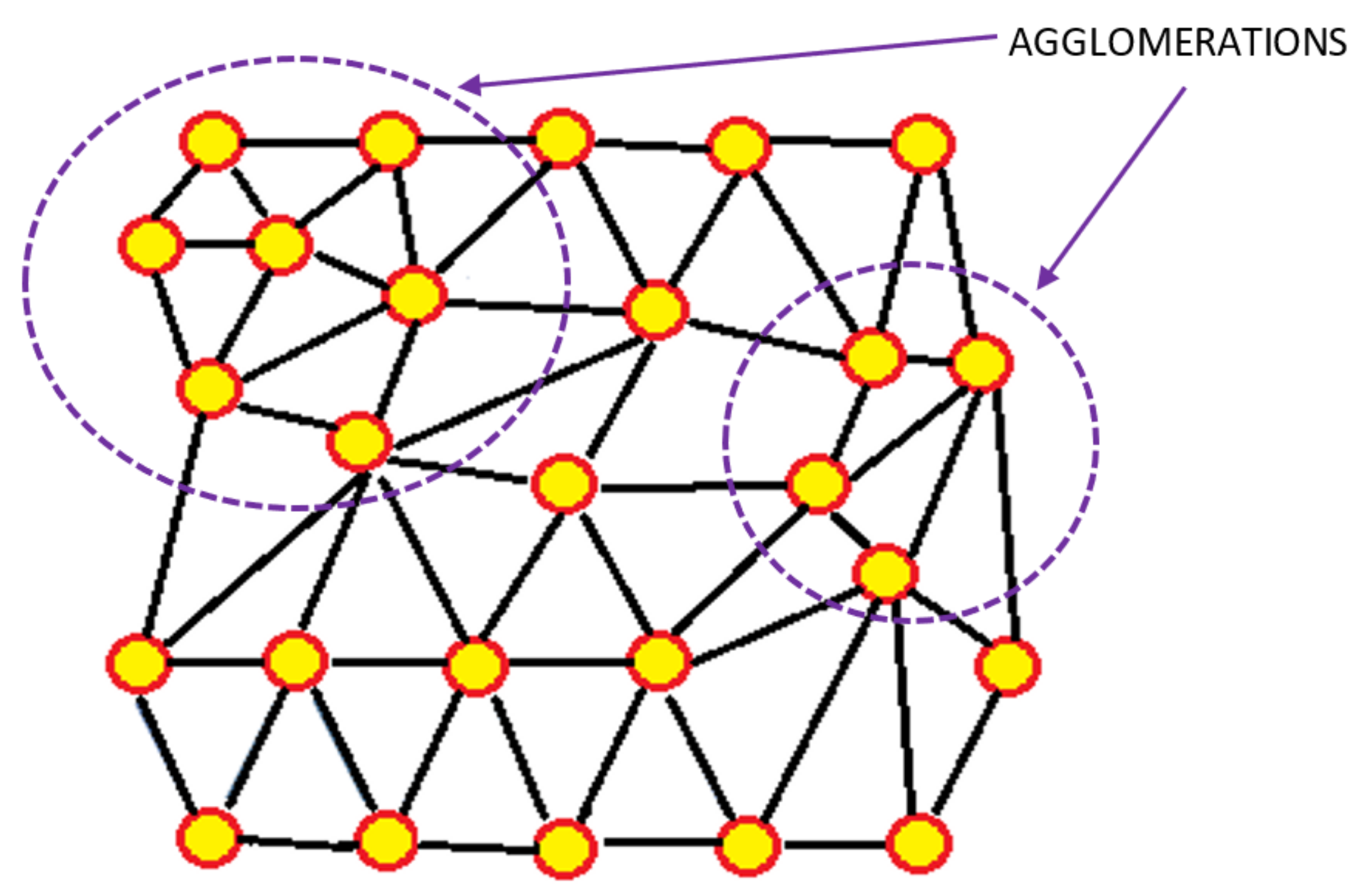
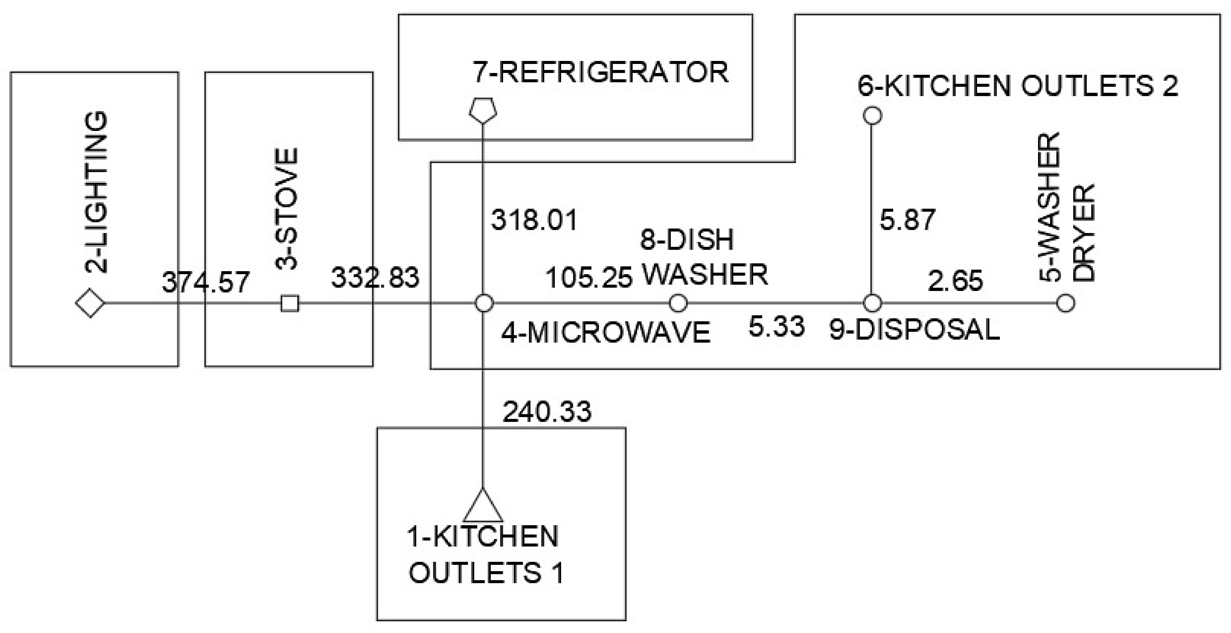
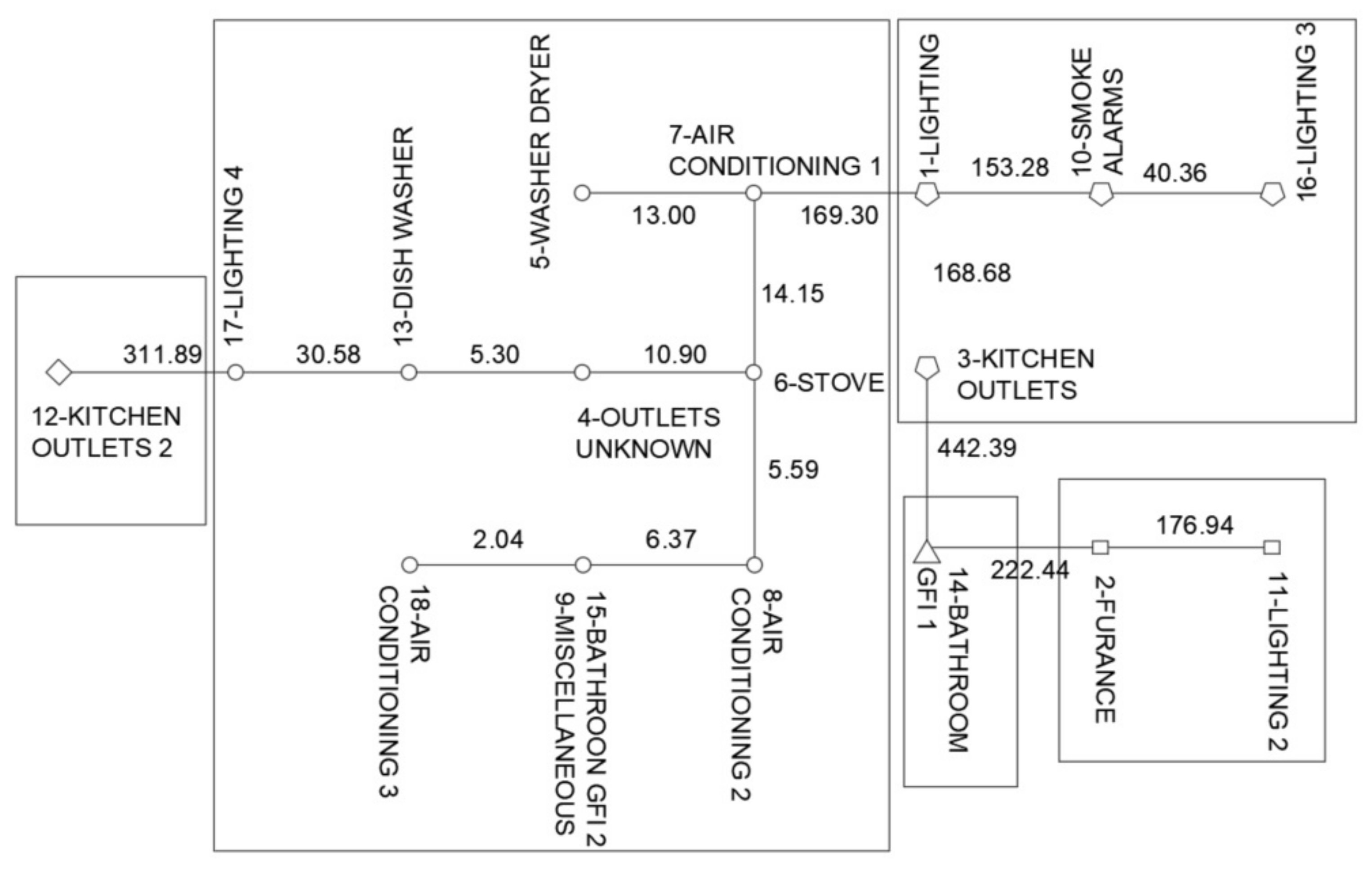
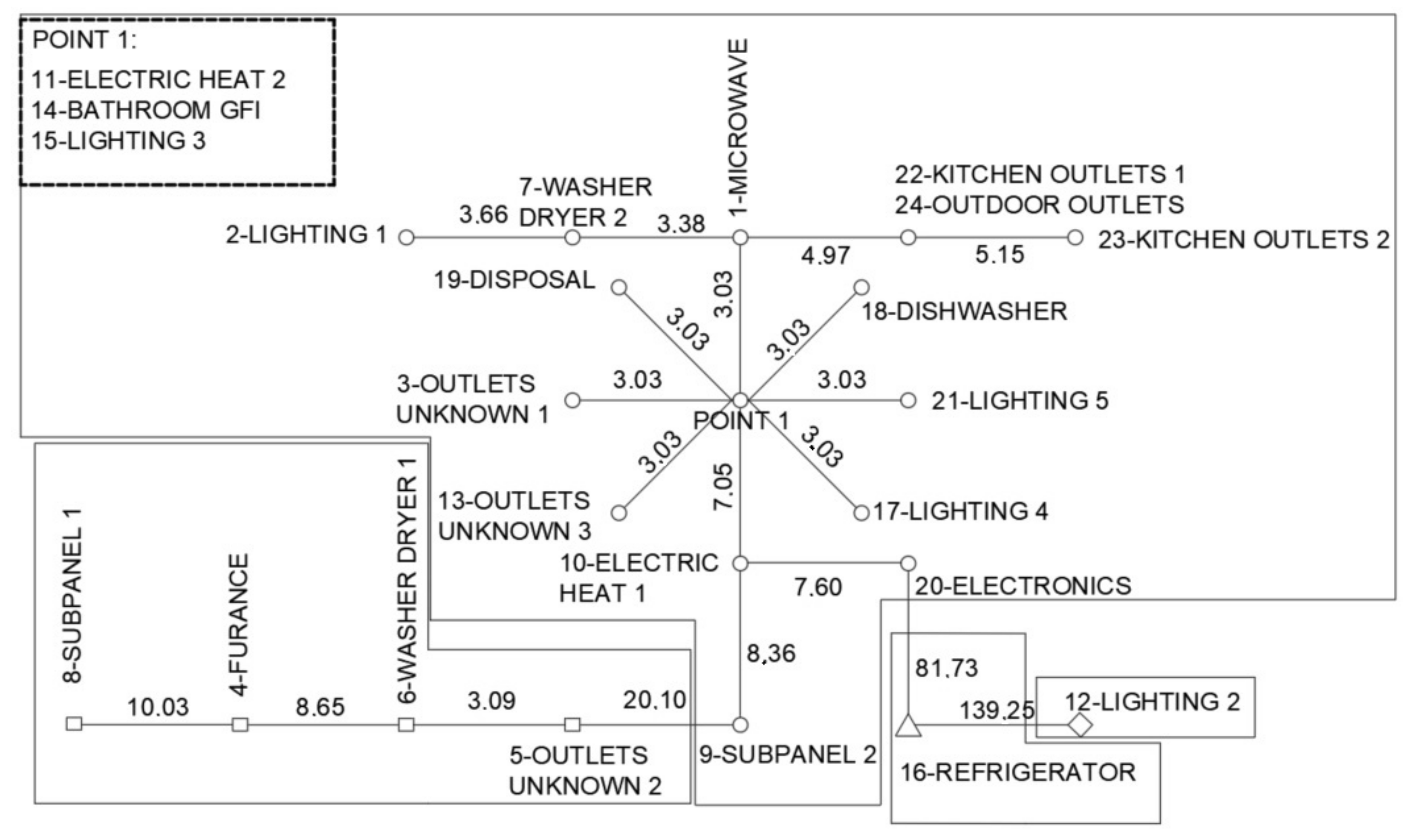
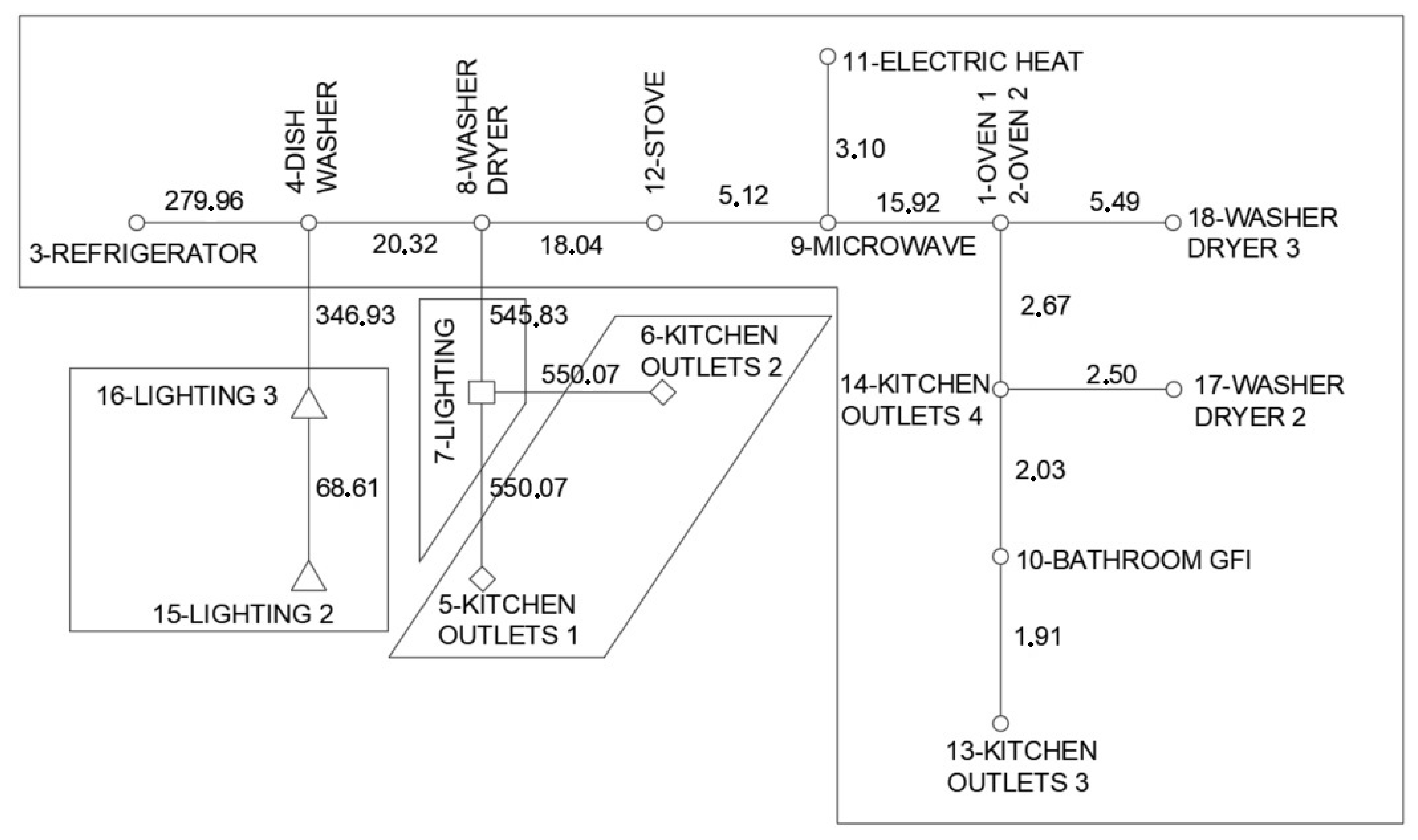
2.2.4. Minimum Spanning Tree

After reducing the problem dimension to ${\mathbb{R}}^3$ and defining the best cluster configuration, a final step was performed to make the clusters easier to visualize. This was made by using the Minimum Spanning Tree [28] for a 3D representation of the results from the PCA.

The Minimum Spanning Tree (MSP) is a tool based on graph theory that gives the shortest path between any two nodes (points) of a connected set. This representation makes it possible to see a 3D result in a 2D figure without any loss of information. Further, the plotting scale can be manipulated to make it possible to visualize distances that are very different in the same picture with the same resolution. The method used to generate the MSP was PRIM [8].

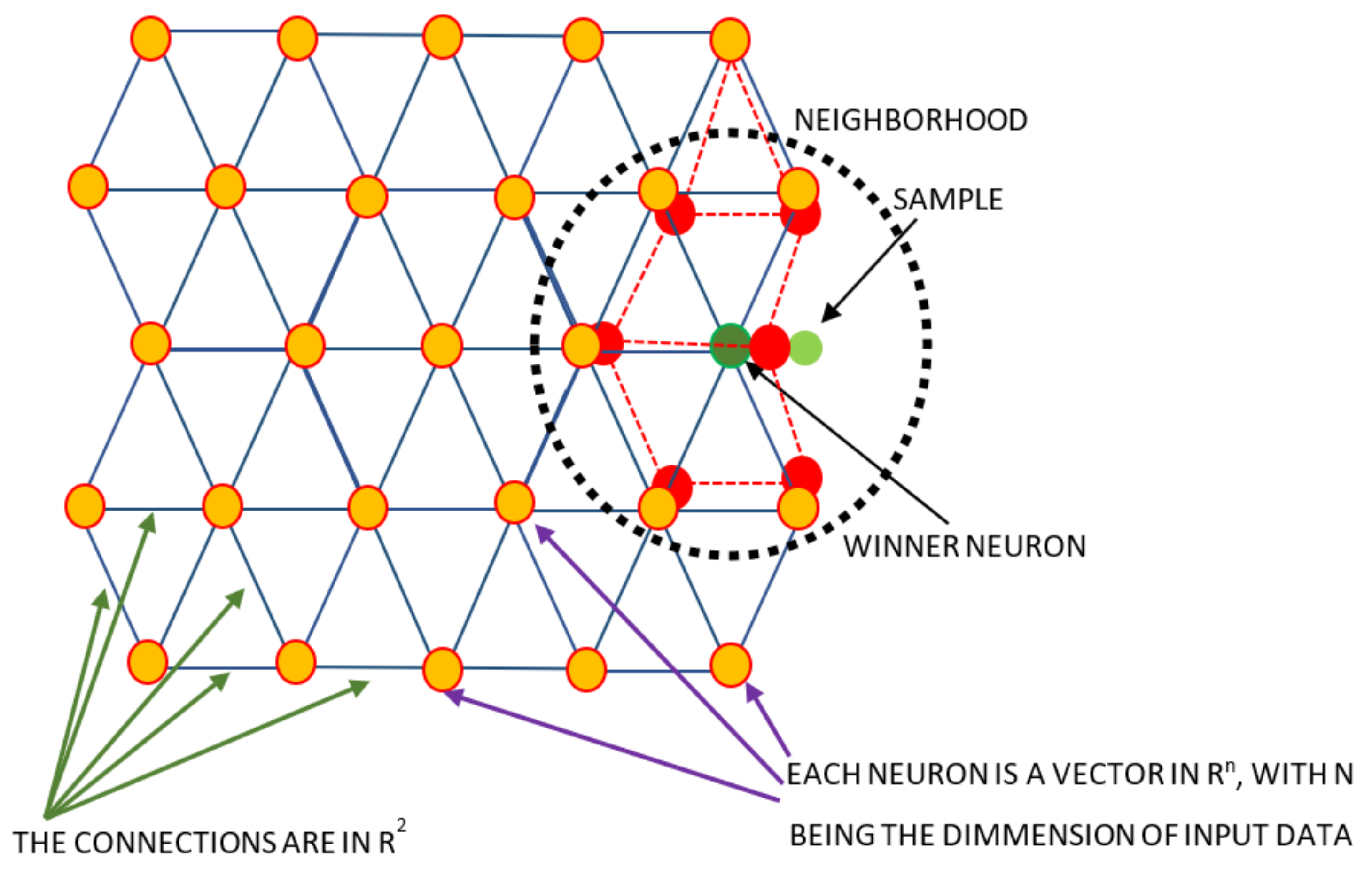
2.2.5. Self Organizing Maps

A Self Organizing Map (SOM) is a tool from the set of unsupervised learning algorithms in machine learning [26]. It consists basically of a grid of neurons that are connected to each other by a specific topography, usually in ${\mathbb{R}}^1$ (linear), ${\mathbb{R}}^2$, or ${\mathbb{R}}^3$. The training of a SOM starts with a predefined number of neurons (in this case, the neuron model is simply a vector in ${\mathbb{R}}^n$, with n being the dimension of the original data). The dimensionality reduction occurs in the connections of the neurons: they are arranged in a linear or two-dimensional way. During the training, the neurons move toward the samples, reflecting agglomerations of similar data that can be observed after the training is finished through all the connections.

The training of a SOM uses the concepts of competitive learning and winner neuron [26]. Thus, when some sample is presented to a map, the neurons will compete to decide which one best represents those specific data. In our case, the neuron closest to the sample (according to the Euclidian distance) will be the winner, and will move toward the sample (see Figure 6). The previous parametrization of the method decides if the winner neuron moves alone or if it also takes the neighbors. One iteration of the training is completed when every sample from the data is presented to the map, and the neurons have moved according to them. After a large number of iterations (hundreds), the neuron structure will show agglomerations that reflect the sample correlations.

After training, the structure of the initially uniformly distributed neurons presents agglomerations that quantitatively indicate a natural classification of the sample set. Referring to Figure 7, some neurons have moved and become very close to each other, whereas other connections have become larger. It is clear that agglomerations exist, which suggests some classification between the samples, but in most cases, a detailed analysis of the distribution of distances is needed to define the groups.

In this case, the Python software was used to apply the SOM algorithm through the SimpSOM library. Because of the machine learning tool, the results depend on the size of the map, the shape (connections between the neurons), and the number of training epochs. Other factors can also influence the final result, but these ones are the most important. To be able to compare the results, a 3D grid with 40 × 40 neurons, hexagonal connections, and 30,000 epochs of training were used for all the datasets.

3. Results

3.1. Linear Method—PCA, k-Means, and MSP

The methodology described in Section 2 was applied to two public datasets: the UK-DALE [13] and the REDD [12] datasets. While in the UK-DALE dataset, there are two houses with a small number of individual channels (Houses 3 and 4 with four and five individual channels, respectively), the period monitored is longer than in the houses in the REDD dataset. This means that as a result, we can expect utilization patterns that are closer to reality than in the REDD [12] dataset. On the other hand, in both cases because of the sampling frequency it is easy to see that the set of system statuses is very redundant as every specific status stays unchanged for several samples. As the samples are made in real houses (instead of being generated by a simulator), the presence of noise in the data is certain. The noisy measurements can, however, be eliminated when the real power value of the individual channels is mapped into a bit status (0 for off and 1 for on).

Considering also that there are 14,400 samples a day for the UK-DALE dataset and 28,800 for the REDD dataset, we have to deal with a total amount of samples, which makes it mandatory to perform redundancy reduction for any further analysis. Even for the house in the UK-DALE with four individual channels and the REDD (with 2.7 monitored days), it is unfeasible to identify the behavior patterns in the raw data. PCA reveals the dynamics involved in the operation patterns of the residential appliances, identifying the appliances that are statistically related. Moreover, as the dimensionality reduction is made by linear transformations, it will not lead to a loss of reference in the appliances.

For all the nine houses analyzed, the first three PCA contained more than 75% of the total set variance. In addition, the total variance in the PCA graph showed a clear elbow around the third Principal Component for all the houses. This means that the dimensionality reduction to ${\mathbb{R}}^3$ performed by PCA is reliable. The results are presented in detail in the following subsections.

3.1.1. UK-DALE—Houses 1, 2, and 5

For the UK-DALE dataset, during the preprocessing phase Houses 3 and 4 were excluded from the present analysis because they have only four and five individual channels, respectively, and the results are thus trivial.

Figure 8, Figure 9 and Figure 10 show the Minimum Spanning Tree resulting from the output of the three principal components of the status set for Houses 1, 2, and 5, respectively. The appliances with distances smaller than one are represented as a single node. The polygons in each figure represent the clusters resulting from the k-means algorithm (with k selected using the elbow method). In House 1, the three first principal components represent an explained variance of 68.81%. Referring to Figure 8, the elbow point is not exactly easy to identify. It could be in any PC from 10 to 15. The 12 first Principal Components were considered to generate the MSTand clusters.

After applying the elbow method for selecting the best number of clusters, the selection of $k=6$ resulted in an explained variance of 93.46%.

The use of PCA in House 2 was very effective. The first three principal components together have an explained variance of 90.18%, and the elbow is defined to be in the fifth PC. The curve of accumulated variance is provided in Figure 11.

The use of the elbow method resulted in the selection of $k=3$ clusters, with explained variance of 99.04%. The Minimum Spanning Tree with the clusters is presented in Figure 9.

For House 5, the three first Principal Components represent an explained variance of 90.97%, the elbow being in PC number 4, with a total accumulated variance of 94.90%. The graph is shown in Figure 12. For the clusters, the elbow method resulted in the selection of $k=4$, with 99.04% percentage of variance explained. The MST and the clusters are represented in Figure 10.

3.1.2. REDD—Houses 1 to 6

The REDD dataset is well organized. Every individual channel has the same quantity of samples. Thus, the algorithm was applied to all the six houses, and the results are shown below. PCA was effective, and in five out of the six houses the first three principal components captured a total variance of more than 80%, confirming that the datasets are very redundant. House 3 showed the lowest rate for the first three PCs, 66.80%, but still this can be considered a reliable result, as presented in

Table 2. Number of individual channels and accumulated variance in the first three PCs set in the REDD data set.

House	Individual Channels	Variance Accumulated by the First 3 PCS [%]
1	18	87.50
2	9	90.97
3	20	66.80
4	18	84.04
5	24	82.72
6	15	94.95

.

The results for the elbow method used to define the best number of clusters are shown in

Table 3. Number of individual channels and time monitored for every house in the REDD data set.

House	Individual Channels	Clusters-k	Variance Accumulated [%]
1	18	4	99.60
2	9	4	97.93
3	20	4	93.95
4	18	5	97.22
5	24	3	97.80
6	15	4	99.6

.

Figure 13, Figure 14, Figure 15 and Figure 16 show the results with k-means for the REDD dataset.

3.2. Nonlinear Method—Self Organizing Maps (SOM)

3.2.1. UK-DALE—Houses 1, 2, and 5

The results shown below were obtained using the SimpSOM library in the Python language and Google Colaboratory to run the code. To make the results comparable, a grid of 40 × 40 neurons was trained for 30,000 epochs with the system status set for each house from the UK-DALE and the REDD datasets. The connections between the neurons follow a hexagonal geometry and the grid is closed. This means that the neurons from the right border of the grid connect to the neurons in the left border, despite the flat figures as an output. The same happens to the upper and lower borders of the grid.

Figure 17a–c show the distances between the grid neurons after the training in a color scale. The neuron agglomerations are represented by dark regions.

3.2.2. REDD—Houses 1 to 6

The same training described for the UK-DALE dataset was applied to the system status set of the REDD houses. The results are shown in Figure 18a–f.

4. Discussion

This work used two different methods of dimensionality reduction to find a natural association between appliances in residential installations. The algorithms were applied in data sets with measurements of actual residences with individual channels from 4 to 52, with monitoring periods from less than three days to more than one month. The data sets selected are the UK-DALE [13] and REDD datasets [12].

4.1. PCA and k-Means for the UK-DALE and the REDD Datasets

In the case of the clusters shown in Figure 19, for the UK-DALE dataset, House 1, the larger group with all the appliances with a significant rated power (soldering iron, dishwasher, and washing machine) indicates a good potential for load modulation. The appliances represented as a single point also provide very interesting results—for example, the soldering iron + kettle—and can be used as a guide for detailed user feedback.

From the clustering results, it is also possible to infer the minimum number of people living in the house. Looking at the type of appliances in the same group, for example, it would be very unlikely that a single person would use several kitchen appliances and the soldering iron at the same time, and thus there should be at least two people in the house at the same time. Following the same logic, the observation of the lights suggests that there are people in the office and the living room during the busy periods.

In the case of the clusters in the UK-DALE dataset, House 2 (see Figure 9), some of the clusters are obvious, such as “modem+server+router”, but the washing machine together with the PlayStation and the other kitchen appliances reveal some habits of the household population that can be exploited. Furthermore, it can be inferred from this result that there are probably three people in the house at that specific moment: one in the kitchen, one using the running machine, and one playing a video game.

In the case of the clusters for the UK-DALE dataset, House 5 (see Figure 10), the group with the office appliances (desktop+sky HD box+core2 server and others) makes a lot of sense, but the group with the kitchen appliances together with the hair dryer, steam iron, and washer dryer suggests that the house has a good load modulation potential. In this case, feedback from the energy supplier to the final user suggesting paying more attention to the use of these appliances together could be advisable. Regarding the number of occupants in the house, it seems that there are at least two people present during the busiest moment, one using the kitchen and the other playing a video game (PS4).

In the case of the clusters for the REDD dataset, House 1 (see Figure 20), the larger group includes almost all the appliances monitored. This means that everything is always used together, despite one lighting circuit (maybe this was always off during the monitoring period) and two circuits of kitchen outlets. House 1 in this data set is an interesting one, because it seems to have three washer dryers. The washer dryer and the dish washer are used together, also with the main appliances such as the stove, microwave, and oven.

In House 2, also for the REDD dataset (see Figure 13), one interesting point about this result is that the refrigerator represents a single cluster, probably because of its very particular “on/off” cycles. Furthermore, this family probably either does not have the habit of cooking (the stove is insulated from the kitchen appliances, but the microwave is very close), or the cooker was broken for the entire monitoring period. Similar analysis could be made for House 3 presented in Figure 21.

The linear approach (PCA and k-means) was very efficient in revealing the existence of appliance clusters. Because of the method’s linearity, the reference in the appliances was not lost during the dimensionality reduction, and the final result is a number of groups for each house, containing appliances that are often used together. The final information can be of great use for the energy suppliers in order to suggest small changes in the consumers’ behavior that can improve the energy efficiency of the residence.

Nevertheless, the main contribution of this method is not only the definition of appliance clusters and the range of analysis options that it brings, but also that the method does not require any information other than a large set of system statuses. If associated with an efficient disaggregation algorithm, the method can extract useful information about the occupants’ behavior by using only the smart meter information.

4.2. Self Organizing Maps for the UK-DALE and REDD Datasets

The method of SOM was used as the nonlinear tool to perform dimensionality reduction and reveal patterns at the same time. Different from PCA and k-means, the SOM results depend on the map size, geometry, and other parameters involving the training itself. The same configuration was used for the nine houses that were analysed in order to obtain comparable results.

Agglomerations of neurons are visible in the grid from the distances between neurons and their neighbours. In our case, this distance is represented by a colour scale: dark blue means closer neurons while light yellow means further ones. In this way, the dark regions in Figure 17a–Figure 18f indicate clusters. For example, in Figure 18e (REDD House 5), three main clusters are visually clear, but in Figure 18c, the map shows agglomerations that could be either interpreted as part of one big cluster or of several small ones. Therefore, the actual number of clusters might not be visually defined in many cases.

Despite this fact, the results of SOM can be considered by following at least two different lines of interpretation. First, if the intention is to compare the linear and nonlinear methods for the same kind of results (finding appliance clusters that are statistically related), another step would be necessary in order to identify which appliances are included in each of the clusters revealed. This, however, would not add much to the conclusions, as the results from PCA are already reliable.

The second line, which is also the main contribution of SOM to this work, follows the fact that the neurons in the dark regions represent system statuses that are very usual, and those in the light regions represent statuses that are not usual. Thus, the trained SOM can be used as a classifier of “usual” or “not usual” system status. If the training is carried out with a sufficiently large set of system statuses that do not contain any malfunctions, the classification can be extended to the “healthy” or “fault or malfunction” statuses.

One very important difference between the SOM and PCA methods is that with PCA, as the method is nonparametric, the interpretation of the results is straightforward. After PCA reduces the data dimensionality, k-means, and the elbow method show the best cluster configuration. On the other hand, this method requires some user inputs, mainly to decide how many PCs will be considered, and the best number of clusters. These can be interpreted as parameters for the whole formulation.

With SOM, first, the grid parameters must be chosen carefully. If the grid is defined to be too small, or there are not enough training epochs, the clusters may not become visible. However, once the parameters are chosen, the result is obtained in only one step: the grid training. Interpretation of the results is not as straightforward as in PCA and k-means, but this gives the reader more liberty to discuss the results in a nonbinary way. For example, in Figure 17a–Figure 18f, the agglomerations are visible, but the number of clusters can be hard to determine exactly.

5. Conclusions

In this paper, we have proposed a technique for the detection of appliance utilization patterns. These patterns are identified from only the system status behavior, which is represented by large system status datasets, by using dimensionality reduction and clustering algorithms. PCA, k-means, and the elbow method are used to define the clusters, and the minimum spanning tree is used to visualize the results and show the appearance of the utilization patterns. The SOM technique is used to create a system status classifier. Thus, the proposed methodology uses low-computational cost algorithms that do not require any information about households.

To demonstrate the effectiveness of the proposed techniques, we applied them to two public datasets from two different countries with different usage patterns—the United Kingdom (UK-DALE) and the US (REDD). The techniques were very effective in revealing the usage patterns of appliances with no need for any personal information of the households.

Using the proposed clustering techniques, system operators can implement effective demand-side management. Further, the system status classifier can be used to detect appliance malfunctions through system status by indicating system statuses that are statistically uncommon. Note, though, that the method does not intend to detect malfunctions as internal short circuits. In the future, we will improve the methodology by incorporating a good performance disaggregation algorithm so that the system status set can be obtained from only the smart meter information, which has received great research attention in the last few years—e.g., [27,29,30,31]. Further, we will improve the classifier formulation, by giving each neuron a label and using the classifier as a real-time monitor. We will try to develop and analyze different classifiers that function seasonally (winter, spring, summer, or autumn) or produce different maps for weekdays and weekends.

In summary, our main objective was to propose a general methodology that can be employed in other datasets and practical setups in a straightforward manner, while also considering possible variations that would require new training periods. In a future paper, we will attempt to generalize this methodology further by applying it to yearly data, as offered by other datasets [32,33], especially taking into account seasonal and other variations.

References

1. García, S.; Parejo, A.; Personal, E.; Guerrero, J.I.; Biscarri, F.; León, C. A retrospective analysis of the impact of the COVID-19 restrictions on energy consumption at a disaggregated level. Appl. Energy 2021, 287, 116547. [Google Scholar] [CrossRef]
2. Vega, A.; Amaya, D.; Santamaría, F.; Rivas, E. Active demand-side management strategies focused on the residential sector. Electr. J. 2020, 33, 106734. [Google Scholar] [CrossRef]
3. Hussain, H.M.; Nardelli, P.H. A Heuristic-based Home Energy Management System for Demand Response. In Proceedings of the 2020 IEEE Conference on Industrial Cyberphysical Systems (ICPS), Tampere, Finland, 10–12 June 2020; Volume 1, pp. 285–290. [Google Scholar]
4. Hui, H.; Ding, Y.; Shi, Q.; Li, F.; Song, Y.; Yan, J. 5G network-based Internet of Things for demand response in smart grid: A survey on application potential. Appl. Energy 2020, 257, 113972. [Google Scholar] [CrossRef]
5. Wei, Y.; Xia, L.; Pan, S.; Wu, J.; Zhang, X.; Han, M.; Zhang, W.; Xie, J.; Li, Q. Prediction of occupancy level and energy consumption in office building using blind system identification and neural networks. Appl. Energy 2019, 240, 276–294. [Google Scholar] [CrossRef]
6. Zhao, H.; Yan, X.; Ren, H. Quantifying flexibility of residential electric vehicle charging loads using non-intrusive load extracting algorithm in demand response. Sustain. Cities Soc. 2019, 50, 101664. [Google Scholar] [CrossRef]
7. Cao, H.Â.; Beckel, C.; Staake, T. Are domestic load profiles stable over time? An attempt to identify target households for demand side management campaigns. In Proceedings of the IECON 2013-39th Annual Conference of the IEEE Industrial Electronics Society, Vienna, Austria, 10–13 November 2013; pp. 4733–4738. [Google Scholar]
8. Chen, Y.C.; Chu, C.M.; Tsao, S.L.; Tsai, T.C. Detecting users’ behaviors based on nonintrusive load monitoring technologies. In Proceedings of the 2013 10th IEEE International Conference on Networking, Sensing and Control (ICNSC), Evry, France, 10–12 April 2013; pp. 804–809. [Google Scholar]
9. Iyengar, S.; Irwin, D.; Shenoy, P. Non-intrusive model derivation: Automated modeling of residential electrical loads. In Proceedings of the Seventh International Conference on Future Energy Systems, Waterloo, ON, Canada, 21–24 June 2016; p. 2. [Google Scholar]
10. Beckel, C.; Sadamori, L.; Staake, T.; Santini, S. Revealing household characteristics from smart meter data. Energy 2014, 78, 397–410. [Google Scholar] [CrossRef] [Green Version]
11. Anderson, K.; Ocneanu, A.; Benitez, D.; Carlson, D.; Rowe, A.; Berges, M. BLUED: A fully labeled public dataset for event-based non-intrusive load monitoring research. In Proceedings of the 2nd KDD Workshop on Data Mining Applications in Sustainability (SustKDD), Beijing, China, 12–16 August 2012; pp. 1–5. [Google Scholar]
12. Kolter, J.Z.; Johnson, M.J. REDD: A public data set for energy disaggregation research. In Proceedings of the Workshop on Data Mining Applications in Sustainability (SIGKDD), San Diego, CA, USA, 21–24 August 2011; Volume 25, pp. 59–62. [Google Scholar]
13. Kelly, J.; Knottenbelt, W. The UK-DALE dataset, domestic appliance-level electricity demand and whole-house demand from five UK homes. Sci. Data 2015, 2, 150007. [Google Scholar] [CrossRef] [PubMed] [Green Version]
14. Allcott, H. Social norms and energy conservation. J. Public Econ. 2011, 95, 1082–1095. [Google Scholar] [CrossRef] [Green Version]
15. Ushakova, A.; Mikhaylov, S.J. Big data to the rescue? Challenges in analysing granular household electricity consumption in the United Kingdom. Energy Res. Soc. Sci. 2020, 64, 101428. [Google Scholar] [CrossRef]
16. Narayanan, A.; De Sena, A.S.; Gutierrez-Rojas, D.; Melgarejo, D.C.; Hussain, H.M.; Ullah, M.; Bayhan, S.; Nardelli, P.H. Key Advances in Pervasive Edge Computing for Industrial Internet of Things in 5G and Beyond. IEEE Access 2020, 8, 206734–206754. [Google Scholar] [CrossRef]
17. Jain, A.K.; Dubes, R.C. Algorithms for Clustering Data; Prentice-Hall, Inc.: Upper Saddle River, NJ, USA, 1988. [Google Scholar]
18. Himeur, Y.; Alsalemi, A.; Bensaali, F.; Amira, A. An intelligent nonintrusive load monitoring scheme based on 2D phase encoding of power signals. Int. J. Intell. Syst. 2021, 36, 72–93. [Google Scholar] [CrossRef]
19. Sa, A.; Thollander, P.; Cagno, E. Assessing the driving factors for energy management program adoption. Renew. Sustain. Energy Rev. 2017, 74, 538–547. [Google Scholar] [CrossRef]
20. Luo, X.; Hong, T.; Chen, Y.; Piette, M.A. Electric load shape benchmarking for small-and medium-sized commercial buildings. Appl. Energy 2017, 204, 715–725. [Google Scholar] [CrossRef] [Green Version]
21. Vercamer, D.; Steurtewagen, B.; Van den Poel, D.; Vermeulen, F. Predicting consumer load profiles using commercial and open data. IEEE Trans. Power Syst. 2015, 31, 3693–3701. [Google Scholar] [CrossRef]
22. Naspolini, H.F.; Rüther, R. The effect of measurement time resolution on the peak time power demand reduction potential of domestic solar hot water systems. Renew. Energy 2016, 88, 325–332. [Google Scholar] [CrossRef]
23. Bucher, C.; Betcke, J.; Andersson, G. Effects of variation of temporal resolution on domestic power and solar irradiance measurements. In Proceedings of the 2013 IEEE Grenoble Conference, Grenoble, France, 16–20 June 2013; pp. 1–6. [Google Scholar]
24. Hernandez, J.; Sanchez-Sutil, F.; Cano-Ortega, A.; Baier, C. Influence of Data Sampling Frequency on Household Consumption Load Profile Features: A Case Study in Spain. Sensors 2020, 20, 6034. [Google Scholar] [CrossRef]
25. Jonathon Shlens, A. Tutorial on Principal Component Analysis http://www.brainmapping.org/NITP/PNA. Readings 2005, 12, 10. [Google Scholar]
26. Haykin, S. Neural Networks and Learning Machines; Pearson Education: London, UK, 2011. [Google Scholar]
27. Hua, D.; Huang, F.; Wang, L.; Chen, W. Simultaneous disaggregation of multiple appliances based on non-intrusive load monitoring. Electr. Power Syst. Res. 2021, 193, 106887. [Google Scholar] [CrossRef]
28. Cheriton, D.; Tarjan, R.E. Finding minimum spanning trees. SIAM J. Comput. 1976, 5, 724–742. [Google Scholar] [CrossRef]
29. Athanasiadis, C.; Doukas, D.; Papadopoulos, T.; Chrysopoulos, A. A Scalable Real-Time Non-Intrusive Load Monitoring System for the Estimation of Household Appliance Power Consumption. Energies 2021, 14, 767. [Google Scholar] [CrossRef]
30. Liu, Y.; Liu, W.; Shen, Y.; Zhao, X.; Gao, S. Toward smart energy user: Real time non-intrusive load monitoring with simultaneous switching operations. Appl. Energy 2021, 287, 116616. [Google Scholar] [CrossRef]
31. Himeur, Y.; Alsalemi, A.; Bensaali, F.; Amira, A. Smart non-intrusive appliance identification using a novel local power histogramming descriptor with an improved k-nearest neighbors classifier. Sustain. Cities Soc. 2021, 67, 102764. [Google Scholar] [CrossRef]
32. Murray, D.; Stankovic, L.; Stankovic, V. An electrical load measurements dataset of United Kingdom households from a two-year longitudinal study. Sci. Data 2017, 4, 1–12. [Google Scholar] [CrossRef] [PubMed] [Green Version]
33. Smith, C.A. The Pecan Street Project: Developing the Electric Utility System of the Future. Ph.D. Thesis, University of Texas, Austin, TX, USA, 2009. [Google Scholar]
Figure 1. Correspondence between the kW sampling and the channel status.
Energies 14 01563 g001
Figure 2. Correspondence between the kW sampling and the channel status.
Energies 14 01563 g002
Figure 3. UK-DALE House 2 preprocessing output file.
Energies 14 01563 g003
Figure 4. Diagram of the proposed method showing the two paths—dimensionality reduction by PCA and clustering by k-means—and the definition of the system status classifier by SOM.
Energies 14 01563 g004
Figure 5. Contribution of variance for each Principal Component, House 2, the UK-DALE data set.
Energies 14 01563 g005
Figure 6. 2D hexagonal geometry and the winner neuron concept. During each training iteration, the winner neuron moves toward the sample and also toward the first neighborhood. The dimensionality reduction occurs because each neuron, a vector in R n , is connected to the other neurons R 2 .
Energies 14 01563 g006
Figure 7. Initial hexagonal SOM after training. When looking at the distances between the neurons, the agglomerations are visible.
Energies 14 01563 g007
Figure 8. UK-DALE, House 1. Variance of each Principal Component and the total variance accumulated. The blue bars represent the individual contribution of each Principal Component, and the orange line represents the total variance accumulated. The elbow is in the 12th Principal Component.
Energies 14 01563 g008
Figure 9. Minimum Spanning Tree for the UK-DALE dataset; House 2 with three clusters defined by the k-means method. The numbers between the nodes (branches) represent the distance considered for generating the Minimum Spanning Tree (branch length). The nodes of each cluster are represented by different shapes and colors (red circle, black lozenge, and green pentagon), and the cluster is also inside a closed polygonal line. The branch representation is not in scale.
Energies 14 01563 g009
Figure 10. Minimum Spanning Tree for the UK-DALE dataset; House 5 with four clusters defined by the k-means method. The numbers between the nodes (branches) represent the distance considered for generating the Minimum Spanning Tree (branch length). The nodes of each cluster are represented by different shapes and colors (red circle, black lozenge, green pentagon, and blue star), and the cluster is also inside a closed polygonal line. The branch representation is not in scale.
Energies 14 01563 g010
Figure 11. UK-DALE, House 2. Variance contribution for each Principal Component, House 2, the UK-DALE data set.
Energies 14 01563 g011
Figure 12. Variance contribution for each Principal Component, House 5, the UK-DALE data set.
Energies 14 01563 g012
Figure 13. Minimum Spanning Tree for the REDD dataset; House 2, with five clusters defined by the k-means method. The numbers between the nodes (branches) represent the distance considered for generating the Minimum Spanning Tree (branch length). The nodes of each cluster are represented by different symbols, and the cluster is also inside a closed polygonal line. The branch representation is not in scale.
Energies 14 01563 g013
Figure 14. Minimum Spanning Tree for the REDD dataset; House 4, with five clusters defined by the k-means method. The numbers between the nodes (branches) represent the distance considered for generating the Minimum Spanning Tree (branch length). The nodes of each cluster are represented by different symbols, and the cluster is also inside a closed polygonal line. The branch representation is not in scale.
Energies 14 01563 g014
Figure 15. Minimum Spanning Tree for the REDD dataset; House 5, with four clusters defined by the k-means method. The numbers between the nodes (branches) represent the distance considered for generating the Minimum Spanning Tree (branch length). The nodes of each cluster are represented by different symbols, and the cluster is also inside a closed polygonal line. The branch representation is not in scale.
Energies 14 01563 g015
Figure 16. Minimum Spanning Tree for the REDD dataset; House 6, with three clusters defined by the k-means method. The numbers between the nodes (branches) represent the distance considered for generating the Minimum Spanning Tree (branch length). The nodes of each cluster are represented by different symbols, and the cluster is also inside a closed polygonal line. The branch representation is not in scale.
Energies 14 01563 g016
Figure 17. 40 × 40 hexagonal SOM after the 30,000 epochs training with the UK-DALE Houses 1, 2, and 5 dataset. The grid geometry is 3D, despite the 2D graphical representation. Thus, the upper horizontal border is connected to the lower horizontal border. The same occurs with the vertical edges. The clusters are represented by dark regions.
Energies 14 01563 g017
Figure 18. 40 × 40 hexagonal SOM after the 30,000 epochs training with the REDD Houses 1 to 6 dataset. The grid geometry is 3D, despite the 2D graphical representation. Thus, the upper horizontal border is connected to the lower horizontal border. The same occurs with the vertical edges. The clusters are represented by dark regions.
Energies 14 01563 g018
Figure 19. UK-DALE, House 1. Clusters as a result of PCA and k-means. Appliances with a distance smaller than 1 are grouped as a single node. The nodes of each cluster are represented by a different symbol (circle, triangle, rectangle, etc).
Energies 14 01563 g019
Figure 20. Minimum Spanning Tree for the REDD dataset; House 1, with four clusters defined by the k-means method. The numbers between the nodes (branches) represent the distance considered for generating the Minimum Spanning Tree (branch length). The nodes of each cluster are represented by different symbols, and the cluster is also inside a closed polygonal line. The branch representation is not in scale.
Energies 14 01563 g020
Figure 21. Minimum Spanning Tree for the REDD dataset; House 3, with five clusters defined by the k-means method. The numbers between the nodes (branches) represent the distance considered for generating the Minimum Spanning Tree (branch length). The nodes of each cluster are represented by different symbols, and the cluster is also inside a closed polygonal line. The branch representation is not in scale.
Energies 14 01563 g021