Development of a Condensation Model and a New Design of a Condensation Hood—Numerical and Experimental Study

Abstract

The development of a numerical model and design for the innovative construction of a heat exchanger (HE) used in a condensation hood (being a part of the combi-steamer) are described in this work. The model covers an air-steam flow, heat transfer, and a steam condensation process. The last two processes were implemented with the use of an in-house model introduced via User Defined Functions (UDF). As the condensate volume is negligible compared to the steam, the proposed model removes the condensate from the domain. This approach enabled the usage of a single-phase flow for both air and steam using a species transport model. As a consequence, a significant mesh and computation time reduction were achieved. The new heat exchanger is characterised by reorganised fluid flow and by externally finned pipes (contrary to the original construction, where internally finned pipes were used). This allowed a reduction in the number of the pipes from 48 to 5, which significantly simplifies construction and manufacturing process of the HE. The redesigned HE was tested in two cases: one simulating normal working conditions with a combi-steamer, the other with extremely high heat load. Measurement data showed that the numerical model predicted condensate mass flow rate (3.67 g/s computed and 3.56 g/s measured) and that the condensation capability increased at least by 15% when compared to the original HE design.

1. Introduction

Technological progress has impacted all areas of life, increasing living standards, wealth, and customer expectations regarding the quality of goods and services applies to the catering sector. As with other industry branches, gastronomy strives to improve cost efficiency, work conditions, quality, and diversity of the served food. A great example of how technology pervades almost every commercial kitchen is a combi-steamer: a device of numerous advantages characterised by its considerable versatility [1]. The combi-steamer utilises steam in dish preparation which is the primary byproduct during work. Odours can accompany the steam, and they can negatively affect the work area, staff, and the meals if not removed promptly after their release [2]. Dedicated infrastructure for the steam and odour removal is expensive and requires the combi-steamer to be in a fixed location. When the oven’s mobility becomes essential for the kitchen to work normally, so-called condensation hoods (CH) come up as a viable and cheaper solution.

Condensation hoods capture the steam produced by the combi-steamers, condense it, and then return it back to the oven by gravitational force. Consequently, additional mobility of the oven is provided, and the water/steam circuit becomes semiclosed. In the ideal case, the condensation hood should condense the whole of the steam and return it to the combi-steamer. Otherwise, the work zone is likely to be contaminated by excessive moisture. Hence, high condensation efficiency is crucial in evaluating of the CHs, for which proper design requires advanced engineering tools, led by computational fluid dynamics (CFD) [3].

The CH, similarly to the combi-steamer, are widely used in gastronomy, but no comprehensive publications nor thorough analyses of these devices are known (according to the authors’ best knowledge). Additionally, a compact design and number of heat and flow processes that take place in this device, make an investigation of such appliance very demanding. A core element of the condensation hood is a heat exchanger (HE)—the part that requires the most manufacturing time and that is the most expensive. This is why an investigation of the HE in terms of a condensation efficiency was the most important task with a lot of potential for improvements.

Although limited when it comes to condensation hoods, the literature describes profusely the unit processes regarding other applications and appliances. The most important phenomena in terms of the condensation efficiency are: the model of condensation of the air-steam mixture coupled with the species transportation process [4,5,6,7,8], the heat transfer in externally-finned pipes with plain circular fins [9,10,11,12,13,14], and also tube bundle configuration analysis [15,16,17,18,19,20,21,22].

This paper is a continuation and extension of the work described by the authors in [23], where a condensation hood original construction (OC) was meticulously examined and appropriate measurements performed. The examined device’s numerical model is then developed and validated successfully in [24]. The numerical model was also used to propose some geometrical improvements to the heat exchanger and as a consequence, a modified construction was developed and used for validation. In the modified construction, a general heat exchanger layout was maintained. The original HE consists of a 48 internally finned pipes organised in a two bundles, where the air flows inside the pipes and the steam outside them. The measurements showed clearly that the bundles are unevenly loaded with the steam. Proposed modifications cover reducing the number of the pipes by 25% and in order to compensate this negative effect, improvements to the steam distribution in the bundles were also included; so both the bundles are more uniformly covered by the steam. Both CH constructions were subjected to validating measurements which showed that both constructions could condensate approximately 3 g/s of the steam. Reducing the number of the pipes significantly limits the production cost of the CH.

In this paper the air-steam flow has been completely reorganised by redesigning the heat exchanger (development of a new construction). The internally finned tubes are replaced by externally finned tubes to enhance convective heat transfer on the air side [16]. As a results, pipe number was reduced from 48 to just 5 and the two pipe bundles were merged into one. Results of simulations considering energy aspects of heat and mass transfer processes occurring in this new design show that the device is able to condensate over 3.5 g/s (somewhat more than original construction). Hence, novelty of this work is twofold: a brand new HE design with completely changed flows of fluids and completely new computational model of the HE implemented as so-called user defined function (UDF). At the same time there is also one similarity to the previous works which consists of replacing the liquid condensate by the mass source (actually mass sink) which closes the mass balance equation for water vapour.

The next section of the paper describes the CH principle of operation. Then details of the computational model are discussed. Results of simulations and discussion are followed by concluding remarks and list of references.

2. Condensation Hood—Operation Principle

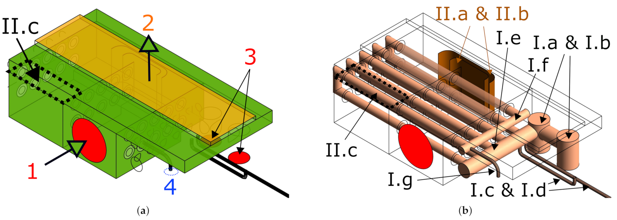
On the left-hand side of Figure 1 is an original design for a CH is presented. On the right-hand side of this figure, the construction of the redesigned heat exchanger is shown. Both devices share the same dimensions, inlet zone with a fan and fan outlet 1, location of the steam vents 3, and air outlet 2. The most important parts of these devices are the heat exchangers indicated by black arrows and dashed lines. The steam produced by the combi-steamer are provided by two steam vents 3 located on one side of each device. In both constructions, the coolant air flows above the upper wall of the HE shell before it leaves the condensation hood through the outlet 2.

In the original construction (Figure 1a), the steam is distributed unequally into two bundles of pipes, where while flowing through the bundle (through the interpipe space), it is cooled and eventually condenses on the pipe’s outer surface. The air absorbs the heat released in this process and is withdrawn from the environment by a fan and pulled through the pipes. The steam, that did not condense, is sucked by the fan, diluted in the coolant air, pulled through the fan outlet 1 to the pipes, and finally released to the environment through the air outlet 2. Because the dominant thermal resistance in the overall heat transfer between steam and air lays on the air-side, the pipes are internally-finned. Such a solution is technologically complex, expensive, and time-consuming in manufacture. There are also problems to guarantee tightness along flow paths in the heat exchanger. A detailed description of the OC can be found in [23,24]. Taking into account all disadvantages of this solution, it seems to be natural to search for a cheaper and simpler construction, while maintaining the condensation efficiency at a comparable level.

In the redesigned construction (RC), pipe bundles were merged and moved to the device’s right-hand side (to the opposite side to the steam vents 3). Instead of flowing into the distribution chamber (space between the bundles where the coolant air is pulled by the fan) and then into the pipes, now the air flows directly into the interpipe space. The total heat transfer surface increased using external fins, that are much thinner and more numerous than their counterparts in the OC. This solution allowed for reduction in the number of the internally finned pipes from 48 to only 5 externally finned. In internally finned pipes, the fins’ number and geometry are limited by the pipe internal diameter cross-section, which made that solution cumbersome and less efficient. In the present case, the primary constraint is only the HE shell dimension, which affects pipe configuration.

The redesigned heat exchanger finally consists of 5 U-shaped horizontal pipes as shown in Figure 2. The pipes are connected by two headers (upper and lower) marked by dashed white lines in Figure 2b,c. The lower header is connected with the steam inlets and provides the steam to the lower pipes. All the pipes and both headers are slightly inclined towards the steam inlets (Figure 2a,b), so the resulting condensate is removed from the CH by the gravitational force back to the oven. The steam condenses inside the pipes while flowing through them. Not condensed water vapour leaves the pipes and flows into the steam exit (Figure 2b,c) being withdrawn by the fan. Then, the steam is in the fan mixed with the air (i.e., diluted) and finally transported to the environment.

It is also worth noting that the fluid flowing inside the pipes close to the steam vents contains mainly steam. Then the condensation process starts, and the resulting liquid condensate has much lower volume than water vapour, which causes that pressure to drop. As a consequence of that process, from space surrounding the fan, some air is sucked and fluid inside the pipes becomes a steam-air mixture. The steam mass fraction in this mixture gradually decreases as the condensation process continues.

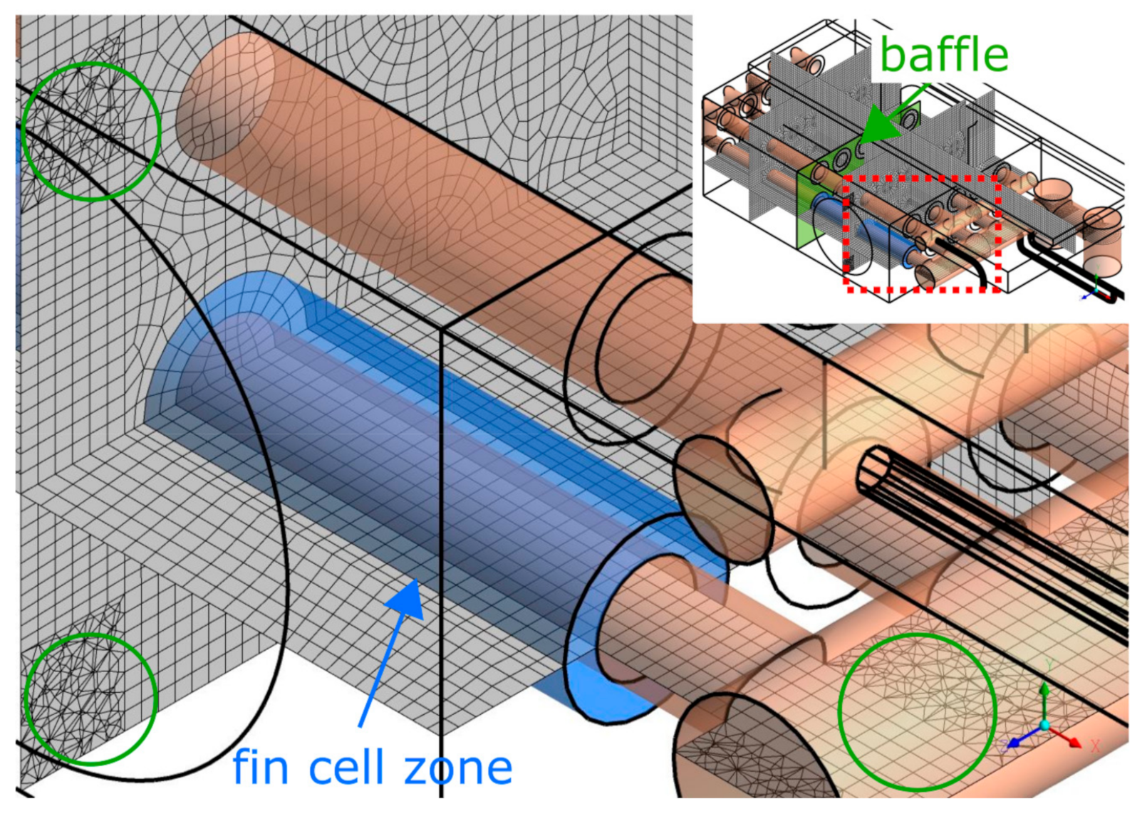
The airflow in the interpipe space (actually between U-shaped pipes) is shown schematically in Figure 2c by the green dashed line. Flow is directed utilising a baffle that divides the pipe space into two sections. Then, once the air reaches the heat exchanger’s rear wall, it is turned by the flow guides and flows again perpendicularly to the pipes. The air leaves the heat exchanger through an outlet II.c marked in Figure 2c by white rectangle (orientation landscape).

3. Condensation Hood—Numerical Model of Processes in the Redesigned Heat Exchanger

The condensation hood’s redesigned heat exchanger is shown schematically in Figure 3. It should be noted that the fan, steam vents, and air outlet location are the same as in previous constructions (i.e., original and modified constructions) [24]. They are all marked in Figure 3a,b together with inlet and outlet conditions as well as paths and zones of the working fluids: 1—air inlet implemented as velocity profile (measured for this new construction together with flow resistance); 2—air outlet implemented as a pressure outlet with porous zone simulating air filter; 3—steam inlets I.a and I.b (steam is provided by combi-steamer); and 4—steam exit I.g implemented as pressure outlet (negative gauge pressure controlled by the fan). The water traps I.c & I.d; lower header, I.e, and upper header I.f are additionally indicated.

The air filter at the air outlet 2 was implemented as a porous zone. Pressure loss measurements of the real filter were conducted for air velocity varying from 1 to 4 m/s. Defining porous zone in Ansys Fluent requires providing two coefficients for each of flow directions: proportionality coefficient and inertial resistance factor. As the flow through the filter is one dimensional, i.e., perpendicular to filter, both coefficients were determined. The remaining components are set as 10${}^3$ times larger. The first parameter was obtained by fitting pressure loss as a function of velocity [25] was adopted.

$$\Delta p=0.154v^2$$

(1)

where $\Delta p$ stands for the pressure loss, v is the air velocity, and proportionality coefficient equal to 0.154 is result of measurements processing.

The polynomial was slightly adjusted in order to keep positive pressure loss values near the minimal measurement range (velocity around 1 m/s). In the next step, the inertial resistance factor $C_2$ is calculated according to the Ansys Fluent User’s Guide [25]

$$C_2=\frac{2·0.154}{\rho \Delta n}$$

(2)

where $\rho =1.16$ stands for the air density, $\mathrm{kg}/{\mathrm{m}}^3$ and $\Delta n=0.013$ is a thickness of the filter, m. Those dates give $C_2=20.44$ which is then introduced to the appropriate viscous resistance direction component.

The flow guide II.a and II.b consists of two plates bent on both sides to evenly distribute the air stream behind the flow guide so that it could interact with the largest possible surface of the pipes. Determination of the dimensions and number of metal sheets in the flow guide was carried out as maximising the uniformity index in Ansys Workbench using Design Exploration Response Surface Optimisation system. The uniformity index accounts for stream distribution on a cross-section of a substrate and can take a value between 0 to 1 (value 0 means nonuniform flow while value 1 stands for ideally uniform flow). Without the flow guide, the uniformity index value was less than 0.5, with two metal sheets in the flow guide, its value increased to 0.78, while with three sheets, the uniformity index took value at around 0.79. The additional metal sheets’ impact was negligible; hence, it was decided to use a flow guide with two sheets only. Surface, where the uniformity index was calculated and maximised, is located the halfway of the heat exchanger section downstream the flow guide.

Slopes of the pipes and the headers are neglected to improve mesh quality. Those elements’ position is an average of extreme positions of their sloped counterparts in the design project visualised in Figure 2. The decision to neglect the slopes also enabled the use of correlations for convective heat transfer for the in-line bundle configuration. Certainly, this approach introduces some minor underestimation regarding the heat transfer coefficients and condensation efficiency, which means the numerical results can be lower than the measured values.

3.1. Main Assumptions and Required Simplifications

This in-house steady-state computational model reduces the number of analysed phases, i.e., only the gas-phase flow was modelled. Liquid condensate resulting from the phase change process was treated as a local mass sink, which closed the mass balance equation for water vapour. The condensation process’s energy effect, i.e., latent heat, was also taken into account in the energy balance.

As it was already mentioned, the heat exchanger in the redesigned construction was equipped with five pipes divided into twenty externally-finned pipe sections. Each section is approximately 480 mm long, which results in approximately 3800 fins in total (0.3 mm fin thickness and 2.24 mm fin pitch). Good quality numerical mesh for such geometry would result in an enormous number of elements, which unfortunately was unacceptable due to computational time and computer memory at our disposal limitations. Consequently, it was decided that simulations of heat and mass transfer processes in the condensation hood heat exchanger should be carried out using a kind of hybrid solution (i.e., superposition of numerical and analytical solutions). In practice, this means that the fins have not been included in the computational domain of the air, so the use of a coarser mesh was allowed in the interfin space, called fin cell zone. The fin cell zone is described further in this section. The convective heat transfer within the interpipe space was solved numerically using relatively coarse numerical mesh and Ansys-Fluent. Heat convection with the steam’s condensation inside the pipe, then heat conduction through the pipe wall and eventually contribution of fins to the convective heat transfer within interfin space, have been modelled analytically using formulae widely known from heat transfer theory. Both solutions are finally superpositioned within interfin space in the way allowing to fulfil energy balance on the external surface of the pipe. These steps of developing an analytical solution and superpositioning it with the numerical solution implemented utilising Fluent’s UDF functionality, requires an appropriate iterative loop.

The developed UDF’s main components are presented schematically in Figure 4. Namely, five main steps can be distinguished: 1—calculation of the heat transfer coefficients for steam and air inside the pipe as well as for the air in the interfin space; 2—determination of the overall thermal resistances for the steam and the air; 3—determination of a maximum heat rates for the steam and for the air; 4—determination of an actual heat transfer rates for the steam and for the air; 5—computation of the source terms.

As a consequence of the UDF implementation (no liquid water), the flow was reduced to a single-phase, which allowed for the employment of the species transport model. The flow consists of two components: the air treated as a single gas (not a mixture of N${}_2$ and O${}_2$) and the steam. Moist air flows in the interpipe space, while the air-steam mixture inside the pipes. In the species transport model the dominant species mass fraction (here: the air) is not calculated from the mass balance equations but is determined as a remaining fraction to close the mass balance ($Y_{air}=1-Y_{H_{2}O}$). As a consequence, the only species transport equation solved by the Fluent concerns the water vapour and takes the form

$$\frac{\partial }{\partial t}\left(\rho Y_{H_{2}O}\right)+\nabla ·\left(\rho \overrightarrow{v}{Y}_{H_{2}O}\right)=-\nabla ·{\overrightarrow{J}}_{H_{2}O}+S_{H_{2}O}$$

(3)

where $Y_{H_{2}O}$ is the water vapour species mass fraction, ${\overrightarrow{J}}_{H_{2}O}$ stands for a water vapour mass diffusion in turbulent flow, and $S_{H_{2}O}$ denotes an additional negative water vapour source defined by the UDF (equal to a condensation source rate ${\dot{m}}_{cond,st}$), $\mathrm{kg}/({\mathrm{m}}^3·\mathrm{s})$, defined in the following sections. Term concerning rate of creation due to chemical reactions in this work is equal to 0 and was not shown in the equation above.

Detailed description of the species transport model, momentum, and energy equations can be found in the Ansys Fluent Theory Guide [26].

Numerical mesh within the interfin space was required to implement the UDF mentioned above, identify local parameters of the air at certain cells, and then calculate coefficients/quantities appearing in the analytical solution. We discuss this in more detail in the next subsections. Discretisation of the interfin space, called fin cell zone, is schematically shown in Figure 5—blue hollow cylinder having external diameter identical as the diameter of the fins and internal diameter equal to the external diameter of the pipe. The CFD solution for the air within the interpipe space SIMPLE scheme was used as a pressure-velocity coupling. Discretisation schemes of pressure, turbulence, species, and energy were set as a second order upwind. Gradient discretisation was set as least squares cell based due to the mesh consisting of mainly hexahedral elements. The analysis was computed with gravitation enabled.

3.2. Heat Transfer Coefficients

To model a film condensation process inside a horizontal tube filled with the steam, the following equation [16] for the heat transfer coefficient $h_{cond}$ (in $\mathrm{W}/({\mathrm{m}}^2·\mathrm{K})$) was employed

$$h_{cond}=0.555{\left[\frac{g{\rho }_{cond}({\rho }_{cond}-{\rho }_{steam})k_{cond}^3}{{\mu }_{cond}\left(T_{sat}-T_{pipe,wall}\right)d_{pipe}}\left(h_{fg}+\frac{3}{8}{C}_{p,cond}\left(T_{sat}-T_{pipe,wall}\right)\right)\right]}^{1/4}$$

(4)

where g stands for gravitational acceleration, $\mathrm{m}/{\mathrm{s}}^2$, ${\rho }_{cond}$ and ${\rho }_{steam}$ are densities of the condensate and the steam, respectively, $\mathrm{kg}/{\mathrm{m}}^3$, $k_{cond}$ denotes condensate’s thermal conductivity, $\mathrm{W}/(\mathrm{m}·\mathrm{K})$, ${\mu }_{cond}$ is a viscosity of the condensate, $\mathrm{kg}/(\mathrm{s}·\mathrm{m})$, $T_{sat}$ and $T_{pipe,wall}$ are steam saturation temperature and the average temperature of the pipe surface, respectively, K, $h_{fg}$ is the heat of vapourisation of the fluid (water), $\mathrm{J}/\mathrm{kg}$, $C_{p,cond}$ denotes the specific heat of the condensate, $\mathrm{J}/(\mathrm{kg}·\mathrm{K})$, and $d_{pipe}$ stands for internal pipe diameter, m.

Equation (4) refers to the steam. However, in the pipes, air also residues, so another heat transfer coefficient, for the air, is needed. To calculate relevant Nusselt number for a turbulent flow in a tube, the Colburn equation [16] was used

$${\mathrm{Nu}}_{air,in}=0.023{\mathrm{Re}}_{air,in}^{0.8}{\mathrm{Pr}}_{air,in}^{\frac{1}{3}}$$

(5)

where ${\mathrm{Nu}}_{air,in}$ stands for the Nusselt number, ${\mathrm{Re}}_{air,in}$ denotes the Reynolds number, and ${\mathrm{Pr}}_{air,in}$ is the Prandtl number. The air properties in the above mentioned dimensionless numbers are calculated at the average air temperature in the considered pipe section defined as

$$T_{air,in,av}=\frac{(T_{air,in,inlet}+T_{air,in,outlet})}{2}$$

(6)

where $T_{air,in,inlet}$ and $T_{air,in,outlet}$ are the mass-weighted average temperatures of the air at the inlet and at the outlet of the pipe section, respectively, K. Finally, the convective heat transfer coefficient for the air inside the tube is derived using the Nusselt number ${\mathrm{Nu}}_{air,in}$

$$h_{air,in}=\frac{{\mathrm{Nu}}_{air,in}{v}_{air,in}}{d_{pipe}}$$

(7)

where $v_{air,in}$ is a mean air velocity in the pipe, $\mathrm{m}/\mathrm{s}$.

The Nusselt number for the finned side of the pipe is based on the correlations for cross flow over tube bundles [16]

$${\mathrm{Nu}}_{air,out}=A{\mathrm{Re}}_{air,out}^b{\mathrm{Pr}}_{air,out}^c{\left(\frac{{\mathrm{Pr}}_{air,out}}{{\mathrm{Pr}}_{pipe,wall}}\right)}^{0.25}$$

(8)

where ${\mathrm{Re}}_{air,out}$ is the Reynolds number defined on the basis of maximum velocity that occurs in the pipe bundle (as the flow cross section area decreases due to existence of the pipes having external diameter $D_{pipe}$), ${\mathrm{Pr}}_{air,out}$ stands for the Prantdl number defined for the temperature $T_{bundle,av}$, while ${\mathrm{Pr}}_{pipe,wall}$ is the Prantdl number defined for the temperature $T_{pipe,wall,av}$. Symbols A, b and c denote correlation coefficients for the in-line bundle arrangement and they depend on the ${\mathrm{Re}}_{air,out}$ value.

The temperature $T_{bundle,av}$ is an arithmetic average temperature of the fluid at the air inlet 1 (i.e., inlet to the bundle) and at the outlet II.c (see Figure 3) which constitutes outlet from the bundle

$$T_{bundle,av}=\frac{T_{bundle,in,av}+T_{bundle,out,av}}{2}$$

(9)

where $T_{bundle,in,av}$ and $T_{bundle,out,av}$ stand for the mass-weighted temperatures of the fluid at the inlet and at the outlet of the bundle, respectively. For instance, temperature $T_{bundle,in,av}$ is calculated according to the following equation

$$T_{bundle,in,av}=\frac{\sum {\rho }_{fin,cell,inlet}{V}_{fin,cell,inlet}{T}_{fin,cell,inlet}}{\sum {\rho }_{fin,cell,inlet}{V}_{fin,cell,inlet}}$$

(10)

where ${\rho }_{fin,cell,inlet}$ stands for the density of the fluid in a cell at the inlet/outlet, $\mathrm{kg}/{\mathrm{m}}^3$, $V_{fin,cell,inlet}$ is the volume of the considered cell, ${\mathrm{m}}^3$, and $T_{fin,cell,inlet}$ denotes for the temperature of the fluid in the cell. All the quantities are provided by the Fluent macros C_R, C_V, and C_T, respectively. Summation is taken over all cells at the inlet and at the outlet surface of the heat exchanger presented in Figure 3 as: 1—air inlet and II.c—air vent. Obviously, temperature $T_{bundle,out,av}$ is determined analogously.

Temperature $T_{pipe,wall,av}$ is calculated as the external pipe wall’s arithmetic mean temperature.

$$T_{pipe,wall,av}=\frac{\sum T_{pipe,wall,face}}{\sum N_{pipe,wall,face}}$$

(11)

where $T_{pipe,wall,face}$ is the temperature of the face adjacent to the pipe wall, K, and $N_{pipe,wall,face}$ stands for the number of faces. The $T_{pipe,wall,face}$ is provided by the Fluent using the F_T macro. Summation is done over all cells at the given pipe wall.

Reynolds number for airflow in the interpipe space ${\mathrm{Re}}_{air,fin}$ is calculated as follows

$${\mathrm{Re}}_{air,fin}=\frac{D_{pipe}{v}_{max}}{\nu }$$

(12)

where $D_{pipe}$ stands for external pipe diameter, $\mathrm{m}$, $v_{max}$ denotes maximum fluid velocity in the bundle, $\mathrm{m}/\mathrm{s}$, and $\nu$ is the kinematic fluid viscosity defined at the temperature $T_{bundle,av}$, ${\mathrm{m}}^2/\mathrm{s}$. The heat transfer coefficient on this side $h_{air,out}$ is calculated separately for the each pipe section depending on the location inside the bundle by introduction of the correction factor F described in [16]

$$h_{air,out}=\frac{F{\mathrm{Nu}}_{air,out}{k}_{air,out}}{D_{pipe}}$$

(13)

where F is the correction factor, –, $k_{air,fin}$ is the fluid thermal conductivity defined in the $T_{bundle,av}$ temperature, $\mathrm{W}/(\mathrm{m}·\mathrm{K})$.

Before the thermal resistances can be computed, the external heat transfer coefficient $h_{air,out}$ needs to be modified to take into account the fins. Hence, a correction factor ${\epsilon }_h$ is calculated according to the following equation

$${\epsilon }_h=\frac{\left((L_{pipe}-N_{fin}{\delta }_{fin})\pi D_{pipe}\right)+\frac{1}{2}\pi N_{fin}\left({(D_{pipe}+2L_{fin})}^2-D_{pipe}^2\right){\eta }_{fin}}{L_{pipe}\pi D_{pipe}}$$

(14)

where $N_{fin}$ stands for the number of fins, ${\delta }_{fin}$ denotes a fin thickness, $\mathrm{m}$, ${\eta }_{fin}$ is a fin efficiency depending on the fin geometry and estimated at 0.95, –, and $L_{fin}$ is a fin length, $\mathrm{m}$.

3.3. Thermal Resistances

Once all the heat transfer coefficients are determined the overall thermal resistances can be computed. Because the air-steam mixture flows in the pipes, there are two overall thermal resistances $R_{air}$ and $R_{steam}$, each one per appropriate mixture component.

$$\begin{array}{c}{R}_{steam}=R_{cond}+R_{pipe}+R_{air,out}=\frac{1}{\pi d_{pipe}{h}_{cond}}+\frac{log\left(\frac{D_{pipe}}{d_{pipe}}\right)}{2\pi k_{pipe}}+\frac{1}{\pi D_{pipe}{h}_{air,out}{\epsilon }_h}\hfill \\ R_{air}=R_{air,in}+R_{pipe}+R_{air,out}=\frac{1}{\pi d_{pipe}{h}_{air,in}}+\frac{log\left(\frac{D_{pipe}}{d_{pipe}}\right)}{2\pi k_{pipe}}+\frac{1}{\pi D_{pipe}{h}_{air,out}{\epsilon }_h}\hfill \end{array}$$

(15)

where $R_{steam}$ and $R_{air}$ are overall thermal resistances of the mixture components, $(\mathrm{m}·\mathrm{K})/\mathrm{W}$ and $k_{pipe}$ denotes thermal conductivity of the pipe, $\mathrm{W}/(\mathrm{m}·\mathrm{K})$. These resistances determine maximal heat fluxes across pipe wall for steam and air, respectively.

3.4. Maximal Heat Transfer Rate

A maximum available heat transfer rate for the air and the steam in a considered section of the pipe ${\dot{Q}}_{max,component}$ equals to

$${\dot{Q}}_{max,component}=\frac{T_{mixture,av}-T_{air,out,av}}{R_{component}}{L}_{pipe}$$

(16)

where $T_{mixture}$ stands for the average temperature of the mixture in the considered pipe section (calculated by the UDF), K, $T_{air,out}$ is an average temperature of the air in the fin cell zone of this pipe section (calculated by the UDF), K, $R_{component}$ is overall thermal resistance of the mixture component $R_{air}$ and $R_{steam}$ (Equation (15)), $(\mathrm{m}·\mathrm{K})/\mathrm{W}$, and $L_{pipe}$ is a length of the pipe section, m.

The temperature of the mixture $T_{mixture}$ is calculated based on cells adjacent to the pipe wall (inside the pipe)

$$T_{mixture,av}=\frac{\sum {\rho }_{pipe,cell,in}{V}_{pipe,cell,in}{T}_{pipe,cell,in}}{\sum {\rho }_{pipe,cell,in}{V}_{pipe,cell,in}}$$

(17)

where ${\rho }_{pipe,cell,in}$ stands for the density of the fluid in a cell adjacent to the pipe wall, $\mathrm{kg}/{\mathrm{m}}^3$, $V_{pipe,cell,in}$ is a volume of the considered cell, ${\mathrm{m}}^3$, and $T_{pipe,cell,in}$ denotes the temperature of the fluid in the cell. All these quantities are provided by the Fluent macros C_R, C_V, and C_T, respectively. Summation is done over all cells at the given section of the pipe wall. The temperature $T_{air,out}$ is computed similarly as $T_{mixture}$; however, the fluid properties come from the cells in the proper fin cell zone.

3.5. Actual Heat Transfer Rates

As the maximum heat transfer rate of the components ${\dot{Q}}_{max,component}$ represents excessive energy carried by the pure one component fluid, it has to be weighted according to the mass fractions of the given components (steam and air) in the mixture

$${\dot{Q}}_{component}=u_{component}{\dot{Q}}_{max,component}$$

(18)

where ${\dot{Q}}_{component}$ stands for heat rate of the component (i.e., steam or the air), W, while $u_{component}$ is a component mass fraction, provided by the Fluent.

3.6. Source Terms

A computational model developed for the heat and mass transfer processes utilises four source terms as discussed in Section 3.1. They are: concerning the condensate, the mass source (actually mass sink) represents condensating water vapour and removing resulting liquid from the computational domain; heat source expressing physical enthalpy of the resulting condensate; and two heat source terms representing the heat transfer rates between the fluid on both sides of the pipe.

The mass sink term ${\dot{m}}_{cond,st}$, in $\mathrm{kg}/(\mathrm{s}·{\mathrm{m}}^3)$ accounts for the amount of the steam which condensed within given cell can be calculated from the following equation

$${\dot{m}}_{cond,st}=-\frac{{\dot{Q}}_{steam}}{h_{fg}^{*}{V}_{cell}}$$

(19)

where $h_{fg}^{*}$ stands for a modified latent heat of vaporisation (accounting for the condensate subcooling), $\mathrm{J}/\mathrm{kg}$, and $V_{cell}$ denotes volume of the analysed numerical cell, ${\mathrm{m}}^3$. The heat transfer rate ${\dot{Q}}_{steam}$ is obtained from Equation (18) while the modified latent heat of vaporisation $h_{fg}^{*}$ is calculated as follows [16]

$$h_{fg}^{*}=h_{fg}+0.68C_{p,l}\left(T_{sat}-T_{wall}\right)$$

(20)

where the $h_{fg}$ is the latent heat in a saturation temperature, $\mathrm{J}/(\mathrm{kg}·\mathrm{K})$, $C_{p,l}$ denotes the specific heat of the liquid at the average film temperature, $\mathrm{J}/(\mathrm{kg}·\mathrm{K})$, $T_{sat}$ and $T_{wall}$ stand for the saturation and wall temperatures, respectively, K.

Along with the mass sink ${\dot{m}}_{cond,st}$, an appropriate energy source term ${\dot{Q}}_{cond,st}$, in $\mathrm{W}/{\mathrm{m}}^3$, needs to be introduced into the energy equation. It represents the physical enthalpy of the condensate which is removed from the computational domain

$${\dot{Q}}_{cond,st}={\dot{m}}_{cond,st}{C}_{p,l}\left(T-T_{Ref}\right)$$

(21)

where T is the fluid temperature in a cell, K, and $T_{Ref}$ is a reference temperature, K.

Heat transferred rate from the air in the pipe to the air in the interpipe space can be treated as a negative source term ${\dot{Q}}_{air,st}$, in $\mathrm{W}/{\mathrm{m}}^3$, and should be considered in energy equation in the pipe

$${\dot{Q}}_{air,st}=-\frac{{\dot{Q}}_{air}}{V_{cell}}$$

(22)

Analogous heat source ${\dot{Q}}_{out,st}$, in $\mathrm{W}/{\mathrm{m}}^3$, but representing the heat transfer rate from the steam-air mixture to the air in the fin cell zone can be determined from the following formula

$${\dot{Q}}_{out,st}=\frac{{\dot{Q}}_{steam}+{\dot{Q}}_{air}}{V_{cell}}$$

(23)

3.7. Model Summary

The developed model constitutes an analytical approach of heat and mass transfer calculation implemented in the numerical model. As presented in Figure 4, five main steps can be distinguished during computational process. At first, the heat transfer coefficients of the condensing steam inside the pipe, the air in the pipe, and the air outside the pipe are computed, according to the Equations (4), (7) and (13), respectively. Next, the overall thermal resistances $R_{steam}$ and $R_{air}$ are calculated as in Equation (15). There are two resistances, because there are two species in the pipes—the steam and the air—which exchange the heat with the coolant air on the outside of the pipes. Once the thermal resistances are known, the maximal heat transfer rates ${\dot{Q}}_{max,component}$ of each species are computed as in the Equation (16), which is common for both species in the model. Equation (16) is suitable in the situation, when the mass fraction of the species equals to 1, which here is not true. Hence, the ${\dot{Q}}_{max,component}$ is mass fraction-weighted as shown in Equation (18) and actual heat transfer rates ${\dot{Q}}_{component}$ (${\dot{Q}}_{steam}$ and ${\dot{Q}}_{air}$) are calculated. At the end, the source terms are derived. There are three source terms that work inside the pipe: ${\dot{m}}_{cond,st}$ which stands for the condensate mass flow rate (Equation (19)), ${\dot{Q}}_{cond,st}$ (Equation (21)) which constitutes a physical enthalpy of the removed condensate due to ${\dot{m}}_{cond,st}$, and ${\dot{Q}}_{air,st}$ from Equation (22) which is the heat transferred between the air inside and outside the pipe, but the source term is applied in the pipe. The last source term, ${\dot{Q}}_{out,st}$ stands for the overall heat that is received by the coolant air outside the pipe and here it is applied.

3.8. Mesh

The numerical mesh, with its discretisation presented in Figure 5, consists of 1.2 million elements, mainly hexahedral. The element’s size is approximately 5 mm and built using the sweep meshing method. Nonsweepable regions meshed with tetrahedral elements are marked with green circles in Figure 5. Those regions are peripheral blocks tangent to a fan boundary condition. Additionally, some sections of the upper and lower header and U-shaped pipe sections are also meshed with tetrahedrons.

Mesh independence analysis showed that the condensate mass flow rate weakly depends on the mesh size, as shown in

Table 1. Mesh independence test.

		Mesh
	Unit:	1	2
Number of elements	—	0.6 × 10${}^6$	1.2 × 10${}^6$
Steam mass flow rate	g/s	11.49	11.49
Condensate mass flow rate	g/s	8.76	8.77

. An extremely high steam load of 11.49 g/s was used as a benchmark. Different meshes were tested, including more fine elements in the fin cell zone and in all cases the mesh density weakly impacted on the condensate flow rate. The final, coarse mesh allows for relatively robust and accurate computations keeping the Y+ at 60–280: 60–80 at the pipe walls and over 200 at the flow guide. As a consequence, the k-$\epsilon$ turbulence model with standard wall functions could be employed.

4. Results and Discussion

The condensation hood equipped with the redesigned heat exchanger was examined in the following two cases:

• A—laboratory conditions, steam provided by a 3.4 kW steam generator,
• B—laboratory conditions, steam provided by a 15 kW steam generator.

Case A corresponds to a typical working conditions, whereas case B constitutes an extremely high heat load that allows one to obtain a maximum possible condensation of the new heat exchanger. Normal working conditions (like in the case A) depend on a mode to which the combi-steamer was set. There are three main modes: convection—base on a hot air (low steam production), combi-steam—mixture of the hot air and the steam (high steam production), and a steam mode—consisting mainly of the steam (high steam production). Both combi-steam and steam modes are comparable in regard of the steam production, which was estimated at approximately 1.0–1.5 g/s and provide much more steam than the convection mode, which produces less than 0.23 g/s [23]. For this reason case A was adjusted so a typical steam production could be maintained during the experiment. The relative humidity of the coolant air ranged from 30 to 40% and the temperature varied from 25 ${}^{\circ }$C to over 30 ${}^{\circ }$C, depending on day.

The condensation hood works in a semi steady-state interrupted by occasional combi-steamer openings in order to insert or withdraw food. Each opening of the tight combi-steamer door releases significant amount of the steam previously accumulated inside. The steam is sucked by the CH in a short period of time, which lasts a couple of seconds until the whole steam is sucked. Such a short deterioration of the coolant air parameters has a serious impact on the CH condensation capability. As a consequence, case B was proposed as a way to examine the maximum condensation capability of the CH.

Results obtained from the experiment and from the numerical model are gathered in

Table 2. Experimental and numerical results: RC—redesigned construction; OC—original construction; Exp—experimental values; CFD—numerical values.

		RC:				OC:
Case:		A		B		A	B*
	Unit:	Exp:	CFD:	Exp:	CFD:	EXP:
$p_{amb}$	Pa	96470		101130
${\phi }_{in}$	%	37.1	39.4	28.8	29.0
$t_{in}$	${}^{\circ }$C	24.5	24.5	31.4	31.4
${\dot{m}}_{air,in}$	kg/s	0.2	0.2	0.2	0.2
$t_{out}$	${}^{\circ }$C	41.7	40	75.2	76.1
${\phi }_{out}$	%	14.4	16.4	7.7	3.52
${\dot{m}}_{steam}$	g/s	1.32	1.32	5.55	5.55	1.18	11.5
${\dot{m}}_{cond}$	g/s	1.29	1.32	3.56	3.67	1.16	3.08
${\eta }_{cond}$	%	97.9	100	64.2	66.1	98.1	26.8

. Inlet quantities measured in the experiment were used as boundary conditions prescribed in the model; hence their experimental and numerical values in the boundary conditions are the same. Numerical values at the outlet are very similar to their experimental counterparts. The most important parameter, condensate mass flow rate ${\dot{m}}_{cond}$ in both cases, is similar. In case A, the experimental condensate mass flow rate was 1.29 g/s, while the numerical prediction is 1.32 g/s. It should be stated that numerical model predicted condensation of almost the whole of the available steam. Because such a limiting situation does not provide reliable information on the model accuracy, it was decided to carry out the experiment for case B, where the steam’s mass flow rate needed to be condensed was much higher. In this case, the steam flow rate was 5.55 g/s, which was almost four times higher than in typical working conditions. The experimental condensate flow rate’s value was equal to 3.56 g/s while the same quantity simulated numerically was 3.67 g/s. These results correspond to 64.2% and 66.1% condensation efficiency ${\eta }_{cond}$, respectively. Both values are fairly close to each other. A similar situation applies to the remaining output or boundary quantities. Hence, it can be concluded that the model is accurate in terms of inlet-outlet values, with a tendency to overestimate the condensation performance slightly.

For performance comparison of RC and OC, Table 2 also contains experimental results obtained for the a case B* (30 kW steam generator) and OC.

The redesigned heat exchanger is a cheaper and simpler alternative to the original construction. It should have, however, at least comparable condensation potential. The condensate mass flow rates of the OC and RC are presented in Table 2. Maximal condensate mass flow rate of the OC has been measured as equal to 3.08 g/s [23] while for RC construction, this quantity is equal to 3.56 g/s, i.e., approx. 16% more. Condensation efficiency ${\eta }_{cond}$ of the OC in a relatively demanding case B* equals almost to 27%, while for the RC it increases to 66% (but for a lower steam flow rate ${\dot{m}}_{steam}$).

It should still be considered that the number of pipes in the heat exchanger was reduced from 48 in the OC to just 5 in the RC. The externally finned pipes used in the RC already were premanufactured and are available at the market, which constitutes significant cost reduction. However, the most problematic parts of the new construction were both headers and to be more specific, the issue of joining them with the pipes while maintaining tightness.

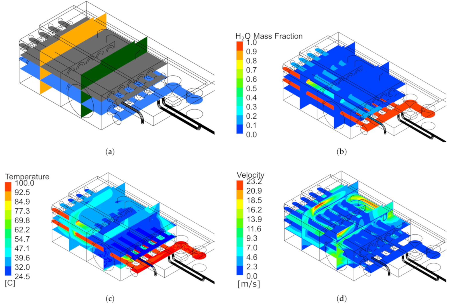
In Figure 6a, the most important cross-sections used for graphical presentation of the field quantities are presented. Cross-sections H1 and H2 are horizontal ones. The first one is located at the height of a lower row of the pipes in such a way that the pipes are crossed along their diameter. The latter one, similarly to H1, crosses upper row of the pipes alongside diameter. There are two remaining cross-sections, V1 and V2, across both sections of the heat exchanger vertically—upstream and downstream the baffle in the middle of the pipes. Figure 6b,c show H${}_2$O mass fraction and temperature distributions inside the device. The steam enters the pipes of the heat exchanger having temperature 100 ${}^{\circ }$C; therefore, highest H${}_2$O mass fraction as well as temperature are located in the steam inlets, lower header, and in the initial sections of the lower pipes. The pipe located farthest from the steam inlets is significantly more loaded, so its lower section and its initial upper section are filled with the hot steam.

Velocity magnitude is presented in Figure 6d. The velocity values range from less than 2.3 m/s inside the pipes (steam and steam-air mixture velocities) to over 20 m/s in the interpipe space, i.e., on the air-side. Such differences between the air and the steam mixture velocities are acceptable because dominant thermal resistance occurs on the air-side, so it is advisable to have relatively high velocities within interpipe space. On steam side, where the velocities are lower by approximately one order of magnitude, condensation occurs; hence the heat transfer rate remains much higher than in the case of forced convection on the air-side.

The steam mass fraction, temperature, and velocity in the H1 cross-section are shown in Figure 7. In Figure 7a,b a nonuniform heat load of the pipes is clearly visible. The majority of the steam flows through the pipe located farthest from the steam inlets. The steam flow rate is great enough that it flows through the whole lower section of this pipe. When considering other pipes, the situation is different. The steam reaches half the length of the lower last but one pipe and less than half of the remaining three pipes closer to the steam inlets. From these figures, the following statement can be formulated: the current design, despite having better condensation performance than the OC, can still be improved by driving the additional pressure drop and forcing more steam to go through the less loaded pipes, for instance, using pipes of different diameters or introducing some orifice meters in the pipes. These options, however, were not tested yet.

Figure 7c presents velocity magnitude in the H1 cross-section. The highest velocity values are in the flow guide region, where the air has to squeeze between the flow guide sheets and radically changes its direction.

Figure 8a,b present steam mass fraction and temperature distributions, respectively but in H2 cross-section, relatively low H${}_2$O mass fraction in the upper pipes (and low in their initial parts) and the temperature; both quantities indicate that there is still a lot of unused heat transfer surface. Contour map of the velocity magnitude is presented in Figure 8c. Velocities below 1 m/s generally occur inside the pipes and up to approximately 20 m/s in the flow guide region. As it can be noted, the uniformity of the velocity profile after the flow guide is not perfect but plausible. Hence, further improvements may include improvement of the flow guide shape and location.

The steam mass fraction, temperature, and velocity magnitude in vertical V1 cross-section are presented in Figure 9. In Figure 9a, it is clearly visible that the steam fills all the lower pipes except two pipes (counting from the right-hand side), where some concentration gradient can be noted. Only in the two upper pipes (counting from the left-hand side) the steam mass fraction is high enough to stand out against the background colour. Steam mass fraction there is up to 30%.

Temperature distribution is presented in Figure 9b. As expected, the air is heated up noticeably only around the lower pipes occupied by the steam. Upper pipes in this cross-section practically do not participate in the heat transfer.

Figure 9c presenting velocity magnitude shows that the air velocity in the bundle reaches about 16 m/s, but between the pipes, row-wise, the velocity reduces to less than 4.6 m/s. However, it should be remembered that the configuration of the pipes in the geometrical model has been simplified by neglecting all the slopes (see Section 3). Hence, the numerical results in terms of velocity field should be treated with some reserve and the model probably also slightly overestimates heat fluxes.

Figure 10 presents distribution of the same quantities but in V2 cross-section. This cross-section is located after the flow guide. Figure 10a presents the steam mass fraction, which is the highest in the pipes located farthest from the steam inlets. In the lower pipe (first to the left), the steam mass fraction is over 90%, while in the upper pipe, it is between 40 and 90%. The H${}_2$O mass fraction in the remaining lower pipes is around 30% while in the remaining upper pipes is ≤20%.

Temperature field in this cross-section presented in the Figure 10b is much more uniform, than in the cross-section V1 in the Figure 9b. The temperature in the majority of sections is at the range 32–40 ${}^{\circ }$C. The highest temperature of approx. 70 ${}^{\circ }$C can be observed right after the first (to the left) lower pipe—the one filled with the steam. Next, hot air flows upwards to near the upper pipe and then leaves the heat exchanger.

Velocity profile shown in Figure 10c is similar to one presented in Figure 9c. In this case, the air still tends to flow between the pipes without thorough flowing around them. As a result, row-wisely regions of low velocity (i.e., ≤2 m/s) are distributed between neighbouring pipes. However, these regions are not as dominant as in Figure 9c. The highest velocity is found right after the air vent II.c.

It should also be noted that to guarantee that the air mass flow rate flowing through the device, being forced by the same fan as in the earlier devices, the II.c vent in RC has been slightly enlarged, and the middle baffle was slightly shortened somewhat to weaken the resistance of the flow bottleneck.

In contrast to the original device, in the redesigned construction the steam flows and is condensed inside the pipes while the cooling air flows through the interpipe space. The pipes are externally finned with plain circular fins.

The basis of all these analyses is the steady-state computational model which accounts for condensation and the heat transfer processes taking place within the heat exchanger. The model has been built using Ansys-Fluent package and its UDF functionality. The UDF utilises the geometry of fins and the appropriate mass and energy sources. Thanks to that approach analysis of complex two-phase flows with a phase change has been substantially simplified and only gas phase could be modelled. The developed model used $k-\epsilon$ turbulence model and accounted for mass balances of air and water including liquid condensate.

5. Conclusions

This paper details, describes, and analyses the new design of the steam-air heat exchanger. This heat exchanger is the essential element of the condensation hood, and it aims to condense steam generated by the combi-steamer during the food preparation process.

Significantly larger heat transfer surface on the air-side allowed for the reduction of the number of the pipes in the heat exchanger from 48 internally-finned (original construction) to just 5 pipes (redesigned construction). Simultaneously, the maximal condensation potential increased from 3.1 g/s (original construction) to almost 3.6 g/s (i.e., by approx. 15%). It should also be stressed that the condensation efficiency of the RC achieves approx. 90%. This effect was achieved with less production effort and can still be improved by more uniform steam distribution in the pipes.

The condensation hood prototype equipped with the redesigned heat exchanger has already been built and tested in the laboratory. Reasonably good agreement between numerical and experimental results allows us to conclude that the developed computational model has been partially validated. Considering the condensation efficiency of this design (approx. 90%) one can also conclude that it is quite an efficient device and can cooperate with a combi-streamer. Moreover, the redesigned heat exchanger still has some potential for further improvements in the fluid flow and heat transfer process.