
Hybrid and Ensemble Methods of Two Days Ahead Forecasts of Electric Energy Production in a Small Wind Turbine

 ,
, 

Abstract
1. Introduction
- Small wind turbines have small rotor inertia, therefore, any change of wind speed instantly affects energy generation;
- Towers of small turbines are low and forecasting of wind speed at low altitudes is burdened with large errors;
- Operation of small turbines can be affected by surrounding obstacles and rough terrain, and energy generation varies due to vegetation or lying snow.
1.1. Related Works
1.2. Objective and Contribution
- Conduct statistical analysis of time series of energy generated from a small wind turbine and potential explanatory variables. Select 8 input data sets to verify how the types and amounts of input data impact on forecasts quality;
- Verify the accuracy of forecasts conducted by single methods, hybrid methods and ensemble methods (18 methods in total);
- Develop and verify an original ensemble method: an averaging ensemble based on hybrid methods without extreme forecasts. Conduct an original selection of combinations of predictors for ensemble methods;
- Indicate the most efficient forecasting methods with no historical wind speed measurements available, but with wind speed forecasts available for up to 48 h ahead.
- This research applies to forecasting of small turbine generation using wind speeds predicted for up to 48 h. This problem is understudies in research so far, especially in comparison with forecasting for large wind farms;
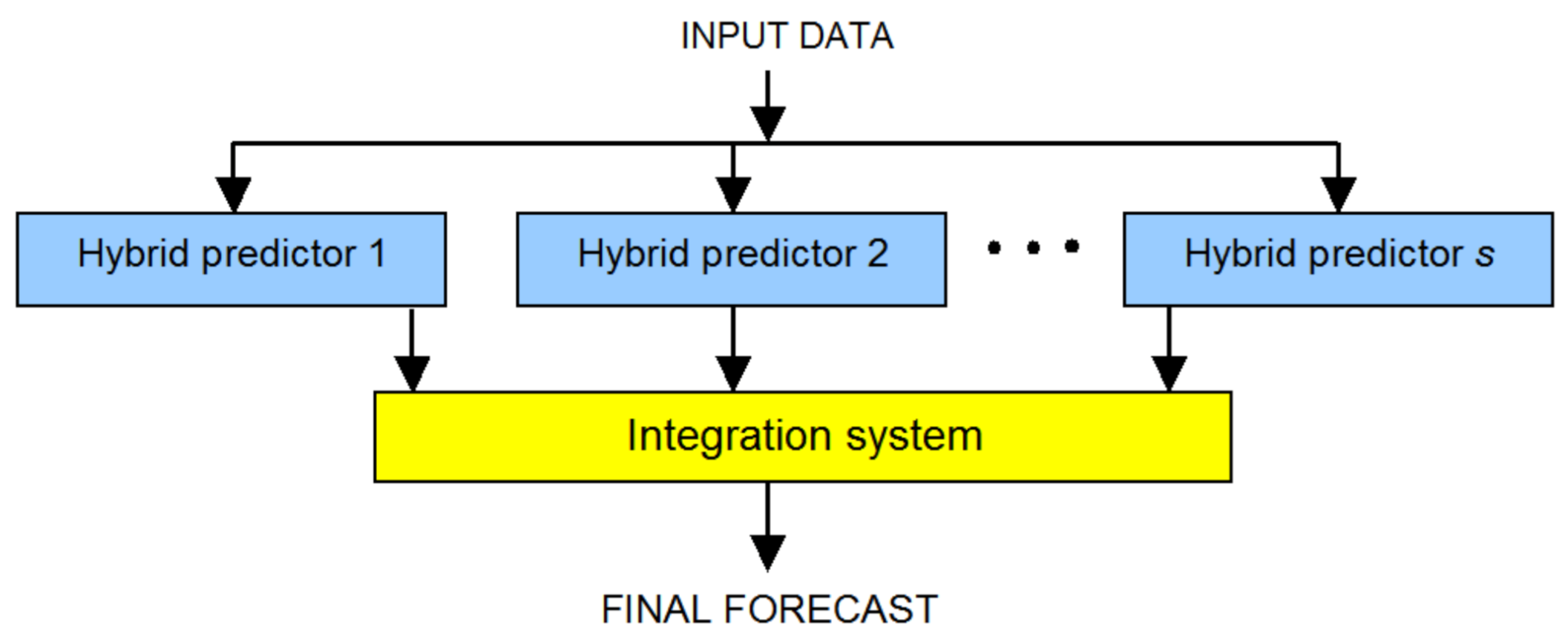
- Development of an ensemble method called “artificial neural network (ANN) type MLP as an integrator of ensemble based on hybrid methods”, which includes a combination of original predictors, and has been arrived at by testing different combinations of predictors. Predictions by this method have yielded the lowest mean absolute error (MAE) among the tested methods;
- Development of an original method called “Averaging ensemble based on hybrid methods without extreme forecasts”. Predictions by this method have yielded the lowest root mean square error (RMSE) among the tested methods;
- Completion of an extensive scenario analysis taking into account different degrees of data availability and model complexities. In total, more than 100 models with different parameters/hyperparameters were tested to choose an optimal model for this complex predictive problem.
2. Data
2.1. Statistical Analysis of Data
2.1.1. Statistical Analysis of Time Series of Hourly Wind Turbine Generations
2.1.2. Statistical Analysis of Wind Speed Forecasts with Horizon from 1 to 48 h
2.2. Selection of Input Data for Particular Forecasting Methods
3. Forecasting Methods
- The BFGS method utilized for solving unconstrained non-linear optimization problems was chosen as a learning algorithm of a neural network (method code MLPBFGS).
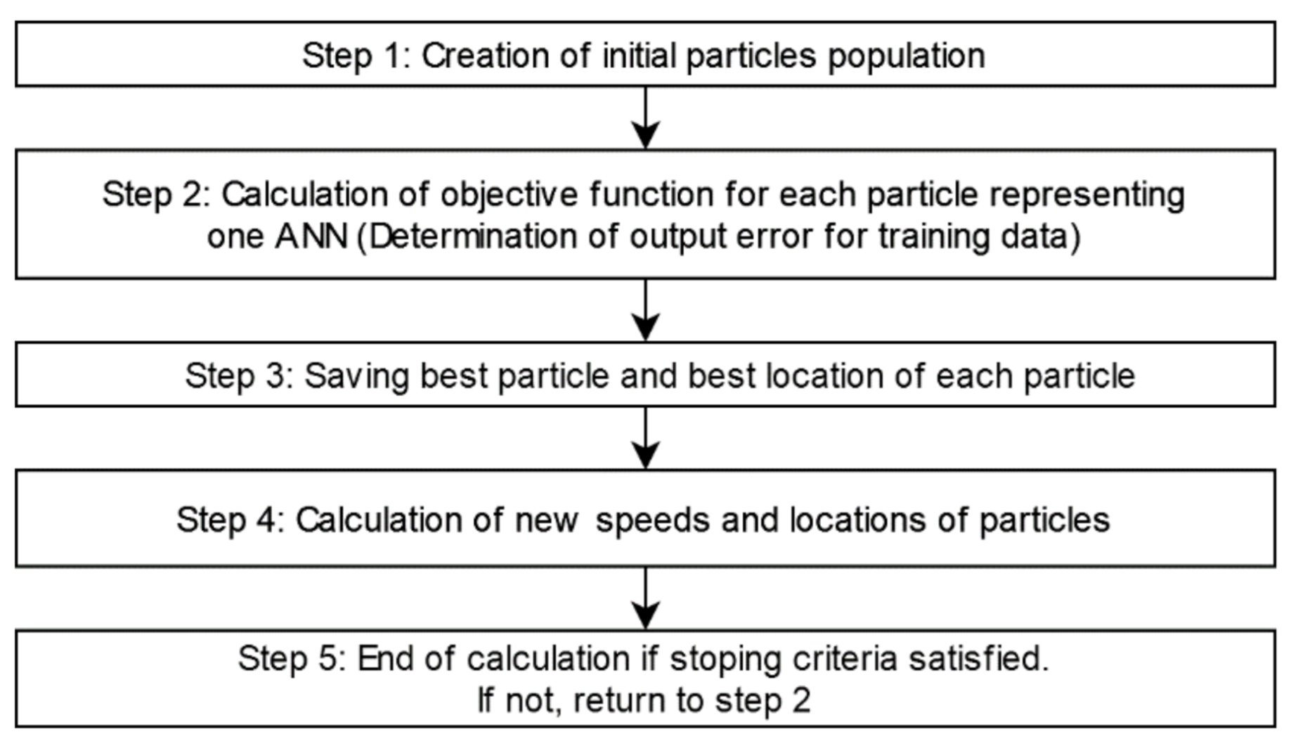
- The particle swarm optimization (PSO) method was used to determine MLP weights (method coded MLPPSO). This hybrid combination of PSO and MLP has been implemented in an original computer program by one of the authors. The following tuning hyperparameters were investigated in our research: number of neurons in hidden layers (5, 8, 10, 20), number of particles in the swarm (20, 50, 100, 150), number of algorithm iterations (100, 1000), coefficients in the formula for particles movements (0.7, 1.0, 1.4), number of iterations between subsequent disturbances in the swarm (50, 100, 400), neighborhood width (2, 5, 10). The optimization concept is presented in Figure 7 and Figure 8.
- Physical model and multiple linear regression model (method code PHM+LR),
- Physical model and K-nearest neighbours regression (method code PHM+KNNR),
- Physical model support vector regression (method code PHM+SVR),
- Physical model and deep neural network type LSTM (method code PHM+LSTM),
- Physical model and artificial neural network type MLP (method codes: PHM+MLBFGS and PHM+MLPPSO).
4. Evaluation Criteria
5. Results and Discussion
- Regarding MAE, qualitative differences between the best two methods (LSTM and MLPPSO) are very small;
- The two clearly worst methods in terms of MAE are NAIVE (the reference method) and SMOOTHING;
- Regarding performance measures for the MLP model, PSO is clearly superior to BFGS as a weight optimization method;
- Values of R are very small and similar for all seven methods, which clearly indicates that single methods with class 1 input data are of little value for the forecasting of wind turbine generation.
- Regarding MAE, qualitative differences between the three best methods (LSTM, LR and MLPPSO) are very small; linear method LR has surprisingly ranked second-best,
- The two clearly worst methods in terms of MAE are SVR and MLPBFGS,
- Regarding performance measures, for the MLP model, PSO is clearly superior to BFGS as a weight optimization method,
- Values of R are very small and similar for all five methods, which clearly indicates that single methods with class 2 input data are of little value for the forecasting of wind turbine generation.
- MAE, RMSE and R have demonstrated clear improvement as compared to the results of Class 2. The reason is that using for Class 3 as an input wind speed forecasts the most important explanatory variable.
- Regarding MAE, qualitative differences between the best three methods (LSTM, MLPPSO and MLPBFGS) are very small,
- In terms of MAE value, PHM is clearly the worst method. This is due to using only wind speed forecasts as input data (set 5),
- The rank of linear method LR by MAE has notably decreased. It is the second worst method in the ranking, so it can be concluded that it is of little value as compared to non-linear methods when wind speed forecasts are included in input data.
- Performance measures have slightly improved as compared to the results of Class 3. This is due to additional use of selected, previously observed values of forecasted time series;
- Taking into account MAE value, qualitative differences among the three best methods (LSTM, MLPPSO and MLPBFGS) are very small;
- MLPBFGS method deserves attention as its RMSE is not only the lowest, but also visibly less than for the LSTM method with the lowest MAE;
- The two clearly worst methods in terms of MAE value are SVR and LR. In particular, linear method LR seems to be of little value.
- Performance measures slightly improved in comparison with results of Class 4. This is due to using a hybrid method—the energy generation forecast from PHM model is additional input data for another, more advanced model;
- Taking into account MAE value, qualitative differences among the two best methods (PHM+LSTM and PHM+MLPPSO) are very small,
- MLPBFGS method deserves attention as its RMSE is the lowest,
- The two clearly worst methods in terms of MAE value are PHM+SVR and PHM+LR. In particular, linear method LR seems to be of little value.
- Performance measures have slightly improved as compared to the results of hybrid methods with input data of Class 5. This is due to the use of different integration systems to achieve the final forecast with the use of selected hybrid methods;
- Taking into account MAE value, qualitative differences among ensemble methods based on hybrid methods are quite small except the last method MIN&MAX_SKIP [PHM+MLPPSO, PHM+LR, PHM+LSTM, PHM+SVR, PHM+KNNR] using 5 hybrid methods;
- Special attention should be paid to MIN&MAX_SKIP [PHM+MLPPSO, PHM+KNNR, PHM+LSTM, PHM+SVR] using 4 instead of 5 hybrid methods (PHM+LR removed from ensemble). MAE of this method is similar to the value for the best method in the MLP_INT [PHM+LSTM, PHM+MLPPSO, PHM+KNNR] ranking. At the same time, it features the lowest RMSE, PCTL75AE, PCTL99AE and the highest value of R.
6. Conclusions
- (1)
- Original hybrid methods and ensemble methods based on hybrid methods, developed for researching specific implementations, have reduced errors of energy generation forecasts for a small wind turbine as compared to single methods.
- (2)
- The best integration system for ensemble methods based on hybrid methods for accuracy measures MAE, R, PCTL75AE and PCTL99AE is a new, original integrator developed for predictions called “averaging ensemble based on hybrid methods without extreme forecasts” (method code MIN&MAX_SKIP) with 3 hybrid methods in the ensemble. This method is notable for its simplicity, especially in contrast with MLP integrator which requires tuning parameters and hyperparameters.
- (3)
- The best integration system in ensemble methods based on hybrid methods for accuracy measure MAE is the MLP integrator.
- (4)
- “An ensemble based on hybrid methods with weight optimization for each predictor” performs better than the method with equal weights for each predictor.
- (5)
- Our research has demonstrated the merits of using ensemble methods based on hybrid methods instead of hybrid methods. Especially, high accuracy gain was achieved as compared to single methods.
- (6)
- Deep neural network LSTM is the best single method, MLP is the second best, while using SVR, KNNR and especially LR is less favorable.
- (7)
- An increase in valuable information in input data (from class 1 to class 5) decreases prediction errors. In particular, wind speed forecasts are the most important input data. Using lagged values of forecast time series proved to slightly increase prediction accuracy. The same applies to using seasonal and daily variability markers.
- (8)
- If lagged values of actual wind velocities can be used as additional input data, the quality of forecasts should slightly improve.
- (9)
- More research is needed to verify, among other things, the following:
- Is prediction accuracy affected by using forecasts from more than one source?
- Does using greater amount of input data, especially wind speed forecasts from periods directly neighboring the forecast period, affect prediction accuracy?
- Will the proposed, original method of “averaging ensemble based on hybrid methods without extreme forecasts” be equally good for different RES predictions from different locations and 1 to 72 h ahead horizons?
Author Contributions
Funding
Institutional Review Board Statement
Informed Consent Statement
Data Availability Statement
Acknowledgments
Conflicts of Interest
Abbreviations
| ACF | Autocorrelation function |
| AE | Absolute Error |
| AM | Attention Mechanism |
| ANFIS | Adaptive Neuro-Fuzzy Inference System |
| ANN | Artificial Neural Network |
| ARIMA-FFNN | Autoregressive Integrated Moving Average—Feedforward Neural Network |
| BFGS | Broyden–Fletcher–Goldfarb–Shanno algorithm |
| BiLSTM-CNN | Bidirectional Long Short Term Memory–Convolutional Neural Network |
| BNN | Bayesian Neural Network |
| DCNN | Deep Convolutional neural network |
| DFFNN | Deep Feed Forward Neural Network |
| DWT | Discrete Wavelet Transform |
| FFT | Fast Fourier Transform |
| GBT | Gradient Boosting Trees |
| KDE | Kernel Density Estimation |
| KNNR | K-Nearest Neighbours Regression |
| LR | Linear Regression |
| LSTM | Long Short-Term Memory |
| LSTM-SARIMA | Long Short-Term Memory–Seasonal Autoregressive Integrated Moving Average |
| MAE | Mean Absolute Error |
| MBE | Mean Bias Error |
| ML | Machine Learning |
| MLP | Multi-Layer Perceptron |
| NWP | Numerical Weather Prediction |
| PCTL75AE | The 75th percentile |
| PCTL99AE | The 99th percentile |
| p.u. | Per unit |
| PV | Photovoltaic System |
| R | Pearson linear correlation coefficient |
| R2 | Determination coefficient |
| RES | Renewable Energy System |
| RF | Random Forests |
| RMSE | Root Mean Square Error |
| RNN | Recurrent Neural Network |
| RSM | Response Surface Method |
| SVR | Support Vector Regression |
| UM | Unified Model |
Appendix A

| Method Code | Description of Method, the Name and the Range of Values of Hyperparameters Tuning and Selected Values |
|---|---|
| PHM+LSTM | The number of hidden layers:1–2, selected:2, the number of neurons in hidden layer: 3–15, selected: 5–5, the activation function in hidden layer: ReLU/ELU/PReLU/LeakyReLU/sigmoid/tanh, selected ReLU, the activation function in output layer: ReLU/sigmoid/tanh/linear, selected tanh, learning algorithm: ADAM, lr = 0.001, decay = 1 × 10⁻⁵, epochs: 2000, patience: 100–500, selected: 100, batch size: 128; shuffle:True. |
| PHM+SVR | Regression SVM: Type-1, Type 2, selected: Type-1, kernel type: Gaussian (RBF), the width parameter σ: 0.333, the regularization constant C, range: 1–20 (step 1), selected: 3, the tolerance ε, range: 0.05–2 (step 0.05), selected: 0.1. |
| PHM+KNNR | Distance metrics: Euclidean, Manhattan, Minkowski, selected: Euclidean, the number of nearest neighbors k, range: 1–200, selected: 42. |
| PHM+MLPPSO | The number of neurons in hidden layers: 5–20, selected 2 hidden layers 10–8, learning algorithm: PSO, the activation function in hidden layer: linear, hyperbolic tangent, selected: hyperbolic tangent, the activation function in output layer: hyperbolic tangent. The number of particles in swarm (20, 50, 100, 150), selected 50, number of algorithm iterations (100, 1000) selected 50, values of coefficients in formula for particles movements (0.7, 1.0, 1.4), selected 1.4 for first coef and 0.7 for the rest, number of iterations between subsequent disturbances in swarm (50, 100, 400), selected 400, neighborhood width (2, 5, 10), selected 5. |
| PHM+MLPBFGS | The number of neurons in hidden layer: 5–20, selected: 13, learning algorithm: BFGS, the activation function in hidden layer: linear, hyperbolic tangent, selected: hyperbolic tangent, the activation function in output layer: linear. |
| MLP_INT [PHM+LSTM, PHM+MLPPSO,PHM+KNNR] | The number of neurons in hidden layer: 3–10, selected: 4, learning algorithm: BFGS, the activation function in hidden layer: linear, hyperbolic tangent, selected: hyperbolic tangent, the activation function in output layer: linear. |
References
- Brodny, J.; Tutak, M.; Saki, S.A. Forecasting the Structure of Energy Production from Renewable Energy Sources and Biofuels in Poland. Energies 2020, 13, 2539. [Google Scholar] [CrossRef]
- Masood, N.A.; Yan, R.; Saha, T.K. A new tool to estimate maximum wind power penetration level: In perspective of frequency response adequacy. Appl. Energy 2015, 154, 209–220. [Google Scholar] [CrossRef]
- Wood, D. Grand Challenges in Wind Energy Research. Front. Energy Res. 2020, 8. [Google Scholar] [CrossRef]
- Hämäläinen, K.; Saltikoff, E.; Hyvärinen, O. Assessment of Probabilistic Wind Forecasts at 100 m Above Ground Level Using Doppler Lidar and Weather Radar Wind Profiles. Mon. Weather Rev. 2020, 8. [Google Scholar] [CrossRef]
- Wilczak, J.M.; Olson, J.B.; Djalalova, I.; Bianco, L.; Berg, L.K.; Shaw, W.J.; Coulter, R.L.; Eckman, R.M.; Freedman, J.; Finley, C.; et al. Data assimilation impact of in situ and remote sensing meteorological observations on wind power forecasts during the first Wind Forecast Improvement Project (WFIP). Wind Energy 2019, 22, 932–944. [Google Scholar] [CrossRef]
- Theuer, F.; van Dooren, M.F.; von Bremen, L.; Kühn, M. Minute-scale power forecast of offshore wind turbines using long-range single-Doppler lidar measurements. Wind Energ. Sci. 2020, 5, 1449–1468. [Google Scholar] [CrossRef]
- Papazek, P.; Schicker, I.; Plant, C.; Kann, A.; Wang, Y. Feature selection, ensemble learning, and artificial neural networks for short-range wind speed forecasts. Meteorol. Z. 2020, 29, 307–322. [Google Scholar] [CrossRef]
- Cai, H.; Jia, X.; Feng, J.; Li, W.; Hsu, Y.M.; Lee, J. Gaussian Process Regression for numerical wind speed prediction enhancement. Renew. Energy 2020, 146, 2112–2123. [Google Scholar] [CrossRef]
- Tawn, R.; Browell, J.; Dinwoodie, I. Missing data in wind farm time series: Properties and effect on forecasts. Electr. Power Syst. Res. 2020, 189, 106640. [Google Scholar] [CrossRef]
- Messner, J.W.; Pinson, P.; Browell, J.; Bjerregård, M.B.; Schicker, I. Evaluation of wind power forecasts—An up-to-date view. Wind Energy 2020, 23, 1461–1481. [Google Scholar] [CrossRef]
- Sewdien, V.N.; Preece, R.; Rueda Torres, J.L.; Rakhshani, E.; van der Meijden, M. Assessment of critical parameters for artificial neural networks based short-term wind generation forecasting. Renew. Energy 2020, 161, 878–892. [Google Scholar] [CrossRef]
- Mishra, S.; Bordin, C.; Taharaguchi, K.; Palu, I. Comparison of deep learning models for multivariate prediction of time series wind power generation and temperature. Energy Rep. 2020, 6, 273–286. [Google Scholar] [CrossRef]
- Shetty, R.P.; Sathyabhama, A.; Pai, P.S. Comparison of modeling methods for wind power prediction: A critical study. Front. Energy 2020, 14, 347–358. [Google Scholar] [CrossRef]
- Spiliotis, E.; Petropoulos, F.; Nikolopoulos, K. The Impact of Imperfect Weather Forecasts on Wind. Power Forecasting Performance: Evidence from Two Wind Farms in Greece. Energies 2020, 13, 1880. [Google Scholar] [CrossRef]
- Baptista, D.; Carvalho, J.P.; Morgado-Dias, F. Comparing different solutions for forecasting the energy production of a wind farm. Neural Comput. Appl. 2020, 32, 15825–15833. [Google Scholar] [CrossRef]
- Hu, J.; Tang, J.; Lin, Y. A novel wind power probabilistic forecasting approach based on joint quantile regression and multi-objective optimization. Renew. Energy 2020, 149, 141–164. [Google Scholar] [CrossRef]
- Zhen, H.; Niu, D.; Yu, M.; Wang, K.; Liang, Y.; Xu, X. A Hybrid Deep Learning Model and Comparison for Wind Power Forecasting Considering Temporal-Spatial Feature Extraction. Sustainability 2020, 12, 9490. [Google Scholar] [CrossRef]
- Ma, Y.-J.; Zhai, M.-Y. A Dual-Step Integrated Machine Learning Model for24 h-Ahead Wind Energy Generation Prediction Based on Actual Measurement Data and Environmental Factors. Appl. Sci. 2019, 9, 2125. [Google Scholar] [CrossRef]
- Zhou, B.; Liu, C.; Li, J.; Sun, B.; Yang, J. A Hybrid Method for Ultrashort-Term Wind Power Prediction considering Meteorological Features and Seasonal Information. Math. Probl. Eng. 2020. [Google Scholar] [CrossRef]
- Chen, K.-S.; Lin, K.-P.; Yan, J.-X.; Hsieh, W.-L. Renewable Power Output Forecasting Using Least-Squares Support Vector Regression and Google Data. Sustainability 2019, 11, 3009. [Google Scholar] [CrossRef]
- Ding, J.; Chen, G.; Yuan, K. Short-Term Wind Power Prediction Based on Improved Grey Wolf Optimization Algorithm for Extreme Learning Machine. Processes 2020, 8, 109. [Google Scholar] [CrossRef]
- Ouyang, T.; Huang, H.; He, Y.; Tang, Z. Chaotic wind power time series prediction via switching data-driven modes. Renew. Energy 2020, 145, 270–281. [Google Scholar] [CrossRef]
- Bracale, A.; Caramia, P.; Carpinelli, G.; De Falco, P. Day-ahead probabilistic wind power forecasting based on ranking and combining NWPs. Int. Trans. Electr. Energy Syst. 2020, 30, 12325. [Google Scholar] [CrossRef]
- Sun, M.; Feng, C.; Zhang, J. Multi-distribution ensemble probabilistic wind power forecasting. Renew. Energy 2020, 148, 135–149. [Google Scholar] [CrossRef]
- Banik, R.; Das, P.; Ray, S.; Biswas, A. Wind power generation probabilistic modeling using ensemble learning techniques. Mater. Today-Proc. 2020, 26, 2157–2162. [Google Scholar] [CrossRef]
- Chen, J.; Zhu, Q.; Li, H.; Lin, Z.; Shi, D.; Li, Y.; Duan, X.; Liu, Y. Learning Heterogeneous Features Jointly: A Deep End-to-End Framework for Multi-Step Short-Term Wind Power Prediction. IEEE Trans. Sustain. Energy 2020, 11. [Google Scholar] [CrossRef]
- Shahid, F.; Khan, A.; Zameer, A.; Arshad, J.; Safdar, K. Wind power prediction using a three stage genetic ensemble and auxiliary predictor. Appl. Soft Comput. 2020, 90, 106151. [Google Scholar] [CrossRef]
- Durán-Rosal, A.M.; Gutiérrez, P.A.; Salcedo-Sanz, S. A statistically-driven Coral Reef Optimization algorithm for optimal size reduction of time series. Appl. Soft Comp. 2018, 63, 139–153. [Google Scholar] [CrossRef]
- Piotrowski, P.; Baczyński, D.; Kopyt, M.; Szafranek, K.; Helt, P.; Gulczyński, T. Analysis of forecasted meteorological data (NWP) for efficient spatial forecasting of wind power generation. Electr. Power Syst. Res. 2019, 175, 105891. [Google Scholar] [CrossRef]
- Yu, M.; Zhang, Z.; Li, X.; Yu, J.; Gao, J.; Liu, Z.; You, B.; Zheng, X.; Yu, R. Superposition Graph Neural Network for offshore wind power prediction. Future Gener. Comput. Syst. 2020, 113, 145–157. [Google Scholar] [CrossRef]
- Fan, H.; Zhang, X.; Mei, S.; Chen, K.; Chen, X. M2GSNet: Multi-Modal Multi-Task Graph Spatiotemporal Network for Ultra-Short-Term Wind Farm Cluster Power Prediction. Appl. Sci. 2020, 10, 7915. [Google Scholar] [CrossRef]
- Li, L.; Li, Y.; Zhou, B.; Wu, Q.; Shen, X.; Liu, H.; Gong, Z. An adaptive time-resolution method for ultra-short-term wind power prediction. Int. J. Electr. Power Energy Syst. 2020, 118, 105814. [Google Scholar] [CrossRef]
- Shahid, F.; Zameer, A.; Mehmood, A.; Raja, M.A.Z. A novel wavenets long short term memory paradigm for wind power prediction. Appl. Energy 2020, 269, 115098. [Google Scholar] [CrossRef]
- Zhang, P.; Li, C.; Peng, C.; Tian, J. Ultra-Short-Term Prediction of Wind Power Based on Error Following Forget Gate-Based Long Short-Term Memory. Energies 2020, 13, 5400. [Google Scholar] [CrossRef]
- Guan, J.; Lin, J.; Guan, J.J.; Mokaramian, E. A novel probabilistic short-term wind energy forecasting model based on an improved kernel density estimation. Int. J. Hydrog. Energy 2020, 45, 23791–23808. [Google Scholar] [CrossRef]
- Géron, A. Hands-on Machine Learning with Scikit-Learn, Keras, and TensorFlow, 2nd ed.; O’Reilly Media, Inc.: Sebastopol, CA, USA, 2019. [Google Scholar]
- Dudek, G.; Pełka, P. Forecasting monthly electricity demand using k nearest neighbor method. Przegląd Elektrotechniczny 2017, 93, 62–65. [Google Scholar]
- Osowski, S.; Siwek, K. Local dynamic integration of ensemble in prediction of time series. Bull. Pol. Ac. Tech 2019, 67, 517–525. [Google Scholar]
- Dudek, G. Multilayer Perceptron for Short-Term Load Forecasting: From Global to Local Approach. Neural Comput. Appl. 2019, 32, 3695–3707. [Google Scholar] [CrossRef]
- Piotrowski, A.P.; Napiorkowski, J.J.; Piotrowska, A.E. Impact of deep learning-based dropout on shallow neural networks applied to stream temperature modelling. Earth-Sci. Rev. 2020, 201, 103076. [Google Scholar] [CrossRef]
- Xie, X.F.; Zhang, W.J.; Yang, Z.L. Social cognitive optimization for nonlinear programming problems. In Proceedings of the International Conference on Machine Learning and Cybernetics (ICMLC), Beijing, China, 4–5 November 2002; pp. 779–783. [Google Scholar]


| Descriptive Statistics | Value |
|---|---|
| Mean | 0.650 [kWh] |
| Standard deviation | 0.899 [kWh] |
| Minimum | 0.000 [kWh] |
| Maximum | 6.684 [kWh] |
| Coefficient of variation | 138.13% |
| The 25th percentile (lower quartile) | 0.000 [kWh] |
| The 50th percentile (median) | 0.364 [kWh] |
| The 75th (upper quartile) | 0.835 [kWh] |
| The 90 percentile | 1.676 [kWh] |
| Variance | 0.808 |
| Skewness | 2.578 |
| Kurtosis | 8.208 |
| Descriptive Statistics | Time Series of Wind Speed Forecasts for up to One Day Ahead (d + 1) | Time Series of Wind Speed Forecasts for the Second Day Ahead (d + 2) |
|---|---|---|
| Mean | 3.592 [m/s] | 3.626 [m/s] |
| Standard deviation | 1.767 [m/s] | 1.750 [m/s] |
| Minimum | 0.088 [m/s] | 0.228 [m/s] |
| Maximum | 11.059 [m/s] | 13.463 [m/s] |
| Coefficient of variation | 49.18% | 48.26% |
| The 25th percentile (lower quartile) | 2.290 [m/s] | 2.377 [m/s] |
| The 50th percentile (median) | 3.284 [m/s] | 3.341 [m/s] |
| The 75th (upper quartile) | 4.672 [m/s] | 4.641 [m/s] |
| The 90 percentile | 6.089 [m/s] | 6.023 [m/s] |
| Variance | 3.121 | 3.063 |
| Skewness | 0.718 | 0.800 |
| Kurtosis | 0.277 | 0.697 |
| Description of Input Data | Code of Input Data | R |
|---|---|---|
| Indicator of annual seasonality—mean daily energy generation for given month | MONTH_I | 0.263 |
| Indicator of daily variability of electric energy production—mean hourly energy generation for given hour | DAY_I | 0.195 |
| Wind speed forecasts—horizons from 1 to 24 h | V_F | 0.756 |
| Wind speed forecasts—horizons from 25 to 48 h | V_F | 0.717 |
| Electric energy production forecast by physical method—the function of polynomial degree 3 | POLY_F | 0.690 |
| Hourly energy generation lagged by 24 h, for 1–24 h horizons | EN_L | 0.343 |
| Hourly energy generation lagged by 48 h, for 25–48 h horizons | EN_L | 0.166 |
| Hourly energy generation lagged by 25 h, for 1–24 h horizons | EN_L-1 | 0.326 |
| Hourly energy generation lagged by 49 h, for 25–48 h horizons | EN_L-1 | 0.161 |
| Hourly energy generation lagged by 26 h, for 1–24 h horizons | EN_L-2 | 0.304 |
| Hourly energy generation lagged by 50 h, for 25–48 h horizons | EN_L-2 | 0.157 |
| Hourly energy generation lagged by 48 h, for 1–24 h horizons | EN_L-24 | 0.166 |
| Hourly energy generation lagged by 72 h, for 25–48 h horizons | EN_L-24 | 0.117 |
| Hourly energy generation lagged by 72 h, for 1–24 h horizons | EN_L-48 | 0.117 |
| Hourly energy generation lagged by 96 h, for 25–48 h horizons | EN_L-48 | 0.161 |
| Name of Set | Description of Set | Codes of Input Data |
|---|---|---|
| Set 1 | Time lag of forecasted time series | EN_L |
| Set 2 | Selected time lags of forecasted time series | EN_L, EN_L-1, EN_L-2 |
| Set 3 | Selected time lags of forecasted time series | EN_L, EN_L-1, EN_L-2, EN_L-24, EN_L-48 |
| Set 4 | - Time lag of forecasted time series - Indicator of annual seasonality - Indictor of variability of daily electric energy production | EN_L, MONTH_I, DAY_I |
| Set 5 | Wind speed forecast | V_F |
| Set 6 | - Indicator of annual seasonality - Indictor of variability of daily electric energy production - Wind speed forecast | MONTH_I, DAY_I V_F |
| Set 7 | - Time lag of forecasted time series - Indicator of annual seasonality - Indictor of variability of daily electric energy production - Wind speed forecast | EN_L, MONTH_I, DAY_I V_F |
| Set 8 | - Time lag of forecasted time series - Indicator of annual seasonality - Indicator of variability of daily electric energy production - Wind speed forecast - Electric energy production forecast by physical model | EN_L, MONTH_I, DAY_I V_F POLY_F |
| The Method Code | Type of Method | Set 1 | Set 2 | Set 3 | Set 4 | Set 5 | Set 6 | Set 7 | Set 8 |
|---|---|---|---|---|---|---|---|---|---|
| NAIVE | Linear | + * | |||||||
| SMOOTHING | Linear | + | |||||||
| PHM | Non-linear | + | |||||||
| LR | Linear | + | + | + | + | ||||
| SVR | Non-linear | + | + | + | + | ||||
| MLPBFGS | Non-linear | + | + | + | + | ||||
| MLPPSO | Non-linear | + | + | + | + | ||||
| LSTM | Non-linear | + | + | + | + | ||||
| PHM+LR | Non-linear | + | |||||||
| PHM+SVR | Non-linear | + | |||||||
| PHM+MLPBFGS | Non-linear | + | |||||||
| PHM+KNNR | Non-linear | + | |||||||
| PHM+MLPPSO | Non-linear | + | |||||||
| PHM+LSTM | Non-linear | + | |||||||
| AVE_INT [PHM+LSTM, PHM+SVR PHM+MLPPSO, PHM+KNNR] | Non-linear | + | |||||||
| AVE_INT [PHM+LSTM, PHM+KNNR, PHM+MLPPSO] | Non-linear | + | |||||||
| W_OPT_INT [PHM+LSTM, PHM+KNNR, PHM+MLPPSO,] | Non-linear | + | |||||||
| W_OPT_INT [PHM+LSTM, PHM+SVR, PHM+MLPPSO, PHM+KNNR,] | Non-linear | + | |||||||
| MIN&MAX_SKIP [PHM+MLPPSO, PHM+KNNR, PHM+LSTM, PHM+SVR] | Non-linear | + | |||||||
| MIN&MAX_SKIP [PHM+MLPPSO, PHM+LR, PHM+LSTM, PHM+SVR, PHM+KNNR] | Non-linear | + | |||||||
| MLP_INT [PHM+LSTM, PHM+MLPPSO, PHM+KNNR] | Non-linear | + |
| Class No. | Description of Input Data | Input Data Sets (Depend on Method) |
|---|---|---|
| Class 1 | Only selected previously observed value of forecasted time series | set 1, set 2, set 3 |
| Class 2 | Selected previously observed values of forecasted time series and indicators of annual seasonality and variability of daily electric energy production | set 4 |
| Class 3 | Wind speed forecast and indicators of annual seasonality and variability of the daily electric energy production (without forecasted time series data) | set 5, set 6 |
| Class 4 | Selected previously observed values of forecasted time series, indicators of annual seasonality and variability of daily electric energy production and wind speed forecast | set 7 |
| Class 5 | Selected previously observed values of forecasted time series, indicators of annual seasonality and variability of the daily electric energy production, wind speed forecast and electric energy production forecast by physical model | set 8 |
| The Method Code | Input Data Set | MAE [kWh] | RMSE [kWh] | MBE [kWh] | PCTL75AE [kWh] | PCTL99AE [kWh] | R |
|---|---|---|---|---|---|---|---|
| LSTM | Set 3 | 0.4841 | 0.8029 | 0.1142 | 0.3632 | 2.7985 | 0.2416 |
| MLPPSO | Set 3 | 0.4842 | 0.8139 | 0.2052 | 0.0954 | 0.5252 | 0.2455 |
| SVR | Set 3 | 0.4975 | 0.8173 | 0.1643 | 0.1151 | 0.8584 | 0.1587 |
| LR | Set 3 | 0.5183 | 0.8556 | 0.3166 | 0.2923 | 1.0914 | 0.2301 |
| MLPBFGS | Set 3 | 0.5304 | 0.9105 | 0.3410 | 0.4291 | 2.9634 | 0.2335 |
| SMOOTHING | Set 2 | 0.6244 | 0.9807 | 0.0323 | 0.4064 | 3.3131 | 0.2260 |
| NAIVE | Set 1 | 0.6336 | 1.0026 | 0.0322 | 0.3997 | 3.6138 | 0.2193 |
| Average measures for single methods with input data class 1 | 0.5389 | 0.8834 | 0.1723 | 0.3002 | 2.1663 | 0.2221 | |
| The Method Code | Input Data Set |
MAE [kWh] | RMSE [kWh] |
MBE [kWh] | PCTL75AE [kWh] | PCTL99AE [kWh] | R |
|---|---|---|---|---|---|---|---|
| LSTM | Set 4 | 0.4788 | 0.7911 | 0.1184 | 0.3491 | 2.6987 | 0.3323 |
| LR | Set 4 | 0.4802 | 0.7927 | 0.1823 | 0.1408 | 0.7133 | 0.3175 |
| MLPPSO | Set 4 | 0.4823 | 0.7983 | 0.2224 | 0.1815 | 0.5256 | 0.3417 |
| SVR | Set 4 | 0.5050 | 0.8280 | 0.2832 | 0.2109 | 0.9387 | 0.2776 |
| MLPBFGS | Set 4 | 0.5204 | 0.8912 | 0.0322 | 0.4114 | 2.9430 | 0.3505 |
| Average performance measures for single methods with input data class 2 | 0.4934 | 0.8203 | 0.1677 | 0.2587 | 1.5639 | 0.3239 | |
| The Method Code | Input Data Set | MAE [kWh] | RMSE [kWh] | MBE [kWh] | PCTL75AE [kWh] | PCTL99AE [kWh] | R |
|---|---|---|---|---|---|---|---|
| LSTM | Set 6 | 0.2860 | 0.4812 | 0.1189 | 0.3520 | 2.7899 | 0.8176 |
| MLPPSO | Set 6 | 0.2902 | 0.4711 | 0.0891 | 0.3693 | 2.7694 | 0.8208 |
| MLPBFGS | Set 6 | 0.2961 | 0.4688 | 0.0328 | 0.4041 | 2.8710 | 0.8177 |
| SVR | Set 6 | 0.3299 | 0.5052 | 0.1448 | 0.2796 | 2.5782 | 0.8064 |
| LR | Set 6 | 0.3562 | 0.5981 | 0.1054 | 0.4612 | 1.2190 | 0.7068 |
| PHM | Set 5 | 0.4389 | 0.6155 | −0.0662 | 0.4691 | 2.7801 | 0.6540 |
| Average performance measures for single methods with input data class 3 | 0.3329 | 0.5233 | 0.0708 | 0.3892 | 2.5013 | 0.7706 | |
| The Method Code | Input Data Set | MAE [kWh] | RMSE [kWh] | MBE [kWh] | PCTL75AE [kWh] | PCTL99AE [kWh] | R |
|---|---|---|---|---|---|---|---|
| LSTM | Set 7 | 0.2854 | 0.4805 | 0.1155 | 0.3514 | 2.7834 | 0.8188 |
| MLPPSO | Set 7 | 0.2909 | 0.4691 | 0.0942 | 0.3717 | 2.6131 | 0.8270 |
| MLPBFGS | Set 7 | 0.2929 | 0.4594 | 0.0293 | 0.4140 | 2.8527 | 0.8253 |
| SVR | Set 7 | 0.3412 | 0.5177 | 0.1474 | 0.2988 | 2.5490 | 0.7937 |
| LR | Set 7 | 0.3531 | 0.6055 | 0.1068 | 0.4512 | 1.2243 | 0.7145 |
| Average performance measures for single methods with input data class 4 | 0.3127 | 0.5064 | 0.0986 | 0.3774 | 2.4045 | 0.7958 | |
| The Method Code | Input Data Set | MAE [kWh] | RMSE [kWh] | MBE [kWh] | PCTL75AE [kWh] | PCTL99AE [kWh] | R |
|---|---|---|---|---|---|---|---|
| PHM+LSTM | Set 8 | 0.2823 | 0.4702 | 0.0830 | 0.3661 | 2.8905 | 0.8202 |
| PHM+MLPPSO | Set 8 | 0.2868 | 0.4727 | 0.0943 | 0.3668 | 2.8300 | 0.8209 |
| PHM+MLPBFGS | Set 8 | 0.2914 | 0.4595 | 0.0329 | 0.4062 | 2.8762 | 0.8260 |
| PHM+KNNR | Set 8 | 0.2996 | 0.4746 | 0.0456 | 0.3763 | 2.6014 | 0.8148 |
| PHM+SVR | Set 8 | 0.3239 | 0.4979 | 0.1294 | 0.2989 | 2.5510 | 0.8088 |
| PHM+LR | Set 8 | 0.3380 | 0.5457 | 0.0984 | 0.3899 | 1.9396 | 0.7677 |
| Average performance measures for hybrid methods with input data class 5 | 0.3037 | 0.4868 | 0.0806 | 0.3674 | 2.6148 | 0.8097 | |
| The Method Code | Input Data Set | MAE [kWh] | RMSE [kWh] | MBE [kWh] | PCTL75AE [kWh] | PCTL99AE [kWh] | R |
|---|---|---|---|---|---|---|---|
| MLP_INT [PHM+LSTM, PHM+MLPPSO, PHM+KNNR] | Set 8 | 0.2816 | 0.4679 | 0.0855 | 0.3650 | 2.7511 | 0.8206 |
| W_OPT_INT [PHM+LSTM, PHM+KNNR, PHM+MLPPSO] | Set 8 | 0.2819 | 0.4681 | 0.0973 | 0.3560 | 2.7173 | 0.8205 |
| AVE_INT [PHM+LSTM, PHM+KNNR, PHM+MLPPSO] | Set 8 | 0.2825 | 0.4701 | 0.0972 | 0.3616 | 2.7871 | 0.8199 |
| MIN&MAX_SKIP [PHM+MLPPSO, PHM+KNNR, PHM+LSTM, PHM+SVR] | Set 8 | 0.2858 | 0.4575 | 0.0844 | 0.3487 | 2.6534 | 0.8259 |
| W_OPT_INT [PHM+LSTM, PHM+SVR, PHM+MLPPSO, PHM+KNNR,] | Set 8 | 0.2860 | 0.4696 | 0.0911 | 0.3563 | 2.8441 | 0.8228 |
| AVE_INT [PHM+LSTM, PHM+SVR, PHM+MLPPSO, PHM+KNNR] | Set 8 | 0.2861 | 0.4708 | 0.0929 | 0.3572 | 2.8479 | 0.8221 |
| MIN&MAX_SKIP [PHM+MLPPSO, PHM+LR, PHM+LSTM, PHM+SVR, PHM+KNNR] | Set 8 | 0.2909 | 0.4677 | 0.0752 | 0.3488 | 2.6536 | 0.8258 |
| Average performance measures for ensemble methods based on hybrid methods with input data class 5 | 0.2850 | 0.4688 | 0.0891 | 0.3562 | 2.7506 | 0.8224 | |
| Class of Method | Method Code | MAE [kWh] | Difference [%] |
|---|---|---|---|
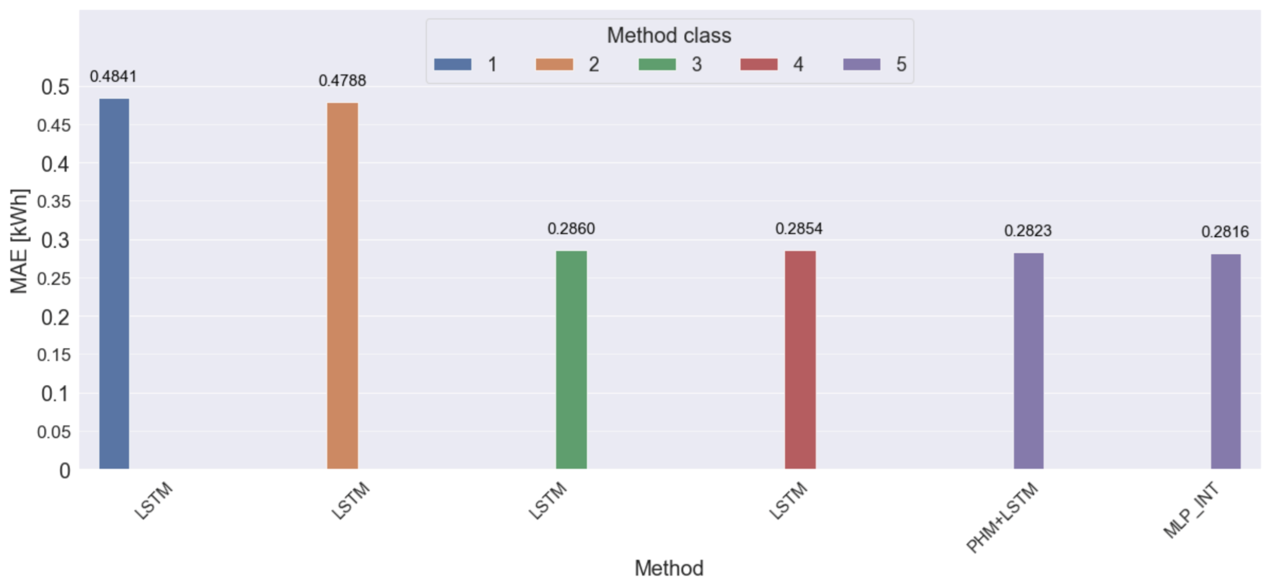
| The ensemble method based on hybrid methods with input data class 5 | MLP_INT [PHM+LSTM, PHM+MLPPSO, PHM+KNNR] | 0.2816 | - |
| The hybrid method with input data class 5 | PHM+LSTM | 0.2823 | 0.25 |
| The single method with input data class 4 | LSTM | 0.2854 | 1.35 |
| The single method with input data class 3 | LSTM | 0.2860 | 1.56 |
| The single method with input data class 2 | LSTM | 0.4788 | 70.03 |
| The single method with input data class 1 | LSTM | 0.4841 | 71.91 |
| Class of Method | Method Code | RMSE [kWh] | Difference [%] |
|---|---|---|---|
| The ensemble method based on hybrid methods with input data class 5 | MIN&MAX_SKIP [PHM+MLPPSO, PHM+KNNR, PHM+LSTM, PHM+SVR] | 0.4575 | - |
| The single method with input data class 4 | MLPBFGS | 0.4594 | 0.42 |
| The hybrid method with input data class 5 | PHM+MLPBFGS | 0.4595 | 0.44 |
| The single method with input data class 3 | MLPBFGS | 0.4688 | 2.47 |
| The single method with input data class 2 | LSTM | 0.7911 | 72.92 |
| The single method with input data class 1 | LSTM | 0.8029 | 75.50 |
Publisher’s Note: MDPI stays neutral with regard to jurisdictional claims in published maps and institutional affiliations. |
© 2021 by the authors. Licensee MDPI, Basel, Switzerland. This article is an open access article distributed under the terms and conditions of the Creative Commons Attribution (CC BY) license (http://creativecommons.org/licenses/by/4.0/).
Share and Cite
Piotrowski, P.; Kopyt, M.; Baczyński, D.; Robak, S.; Gulczyński, T. Hybrid and Ensemble Methods of Two Days Ahead Forecasts of Electric Energy Production in a Small Wind Turbine. Energies 2021, 14, 1225. https://doi.org/10.3390/en14051225
Piotrowski P, Kopyt M, Baczyński D, Robak S, Gulczyński T. Hybrid and Ensemble Methods of Two Days Ahead Forecasts of Electric Energy Production in a Small Wind Turbine. Energies. 2021; 14(5):1225. https://doi.org/10.3390/en14051225
Chicago/Turabian StylePiotrowski, Paweł, Marcin Kopyt, Dariusz Baczyński, Sylwester Robak, and Tomasz Gulczyński. 2021. "Hybrid and Ensemble Methods of Two Days Ahead Forecasts of Electric Energy Production in a Small Wind Turbine" Energies 14, no. 5: 1225. https://doi.org/10.3390/en14051225
APA StylePiotrowski, P., Kopyt, M., Baczyński, D., Robak, S., & Gulczyński, T. (2021). Hybrid and Ensemble Methods of Two Days Ahead Forecasts of Electric Energy Production in a Small Wind Turbine. Energies, 14(5), 1225. https://doi.org/10.3390/en14051225