Online Quality Measurements of Total Suspended Solids for Offshore Reinjection: A Review Study

 , , and
Abstract
1. Introduction
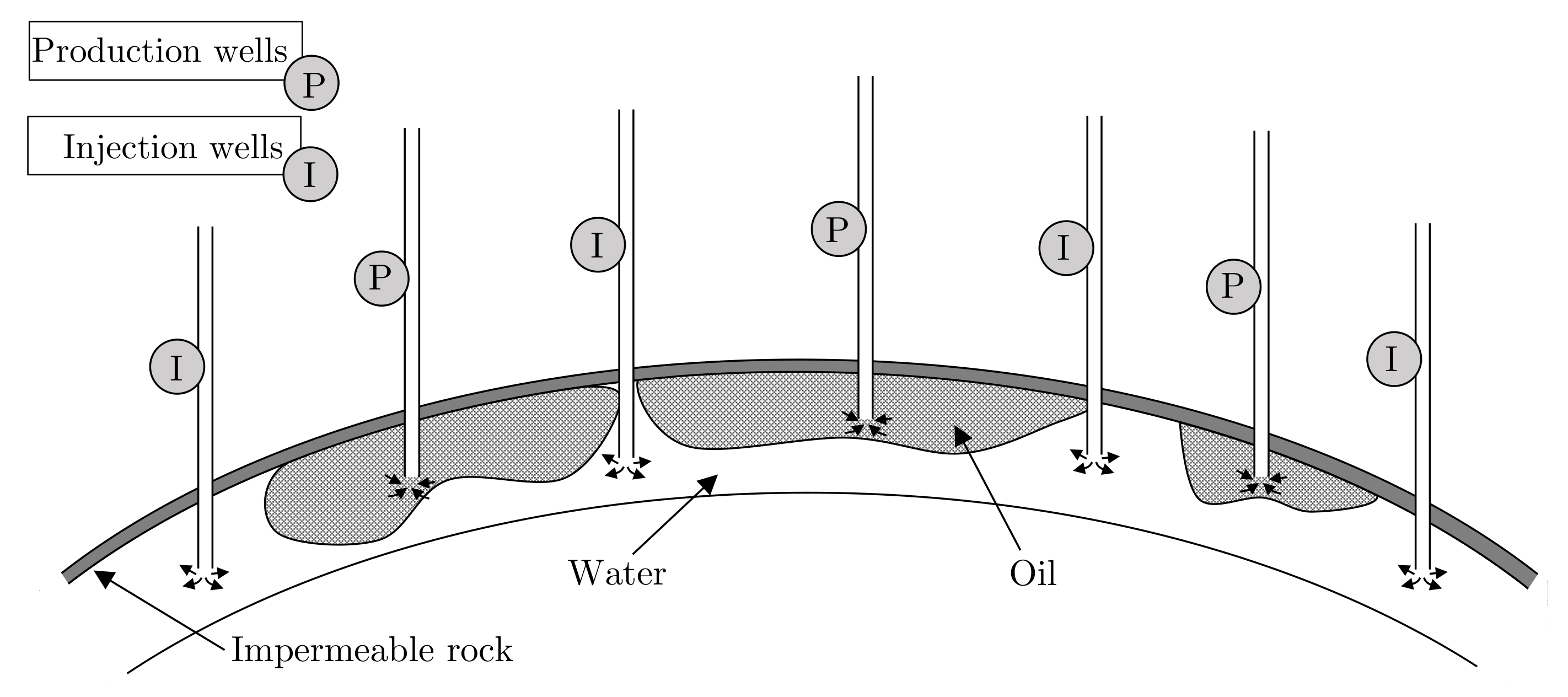
2. Waterflooding
“The additional recovery of oil from a petroleum reservoir over that which can be economically recovered by conventional primary and secondary methods”.[13]
- Primary oil recovery: ~10–15% of OIP
- Secondary oil recovery: ~15–33% of OIP
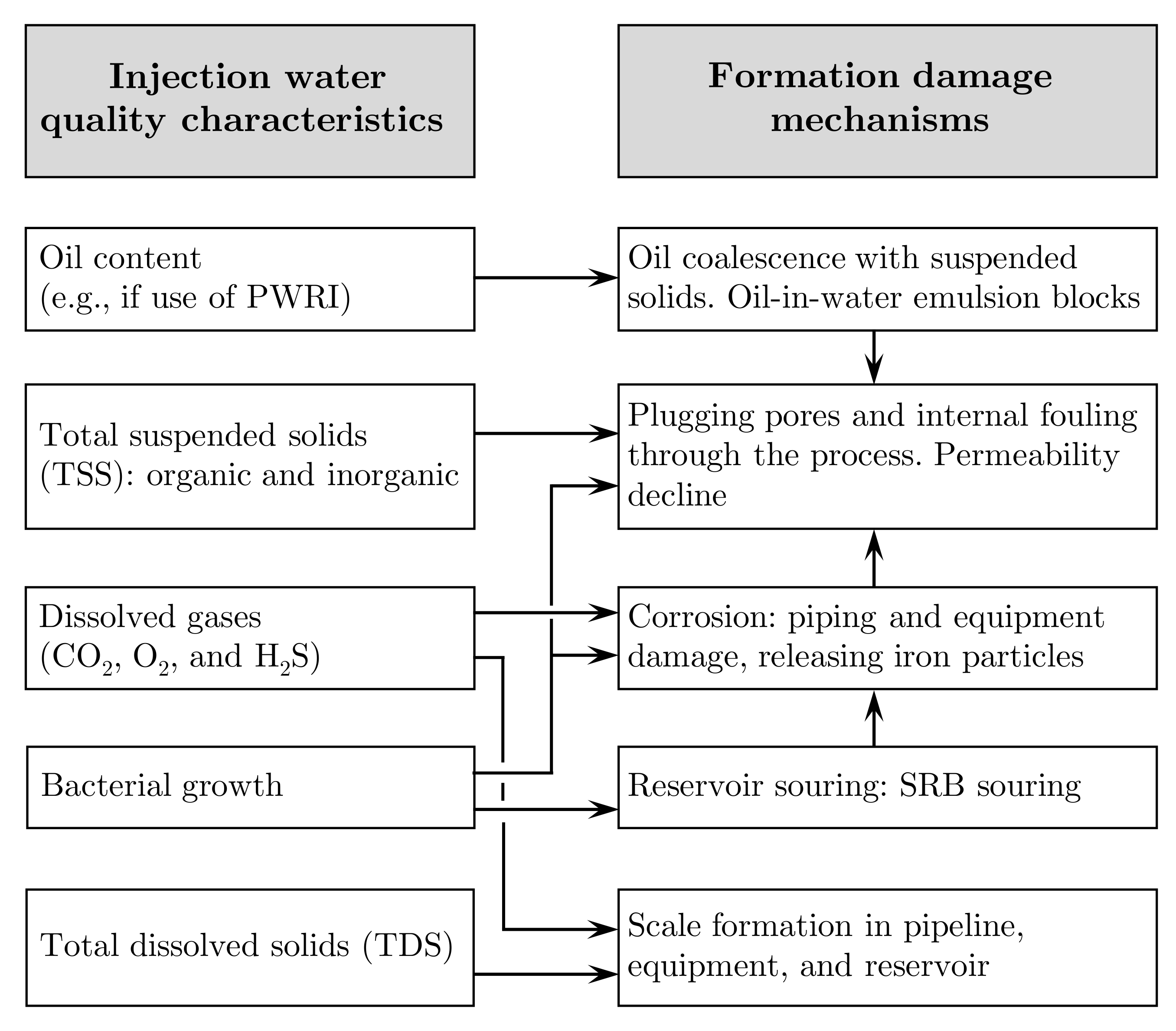
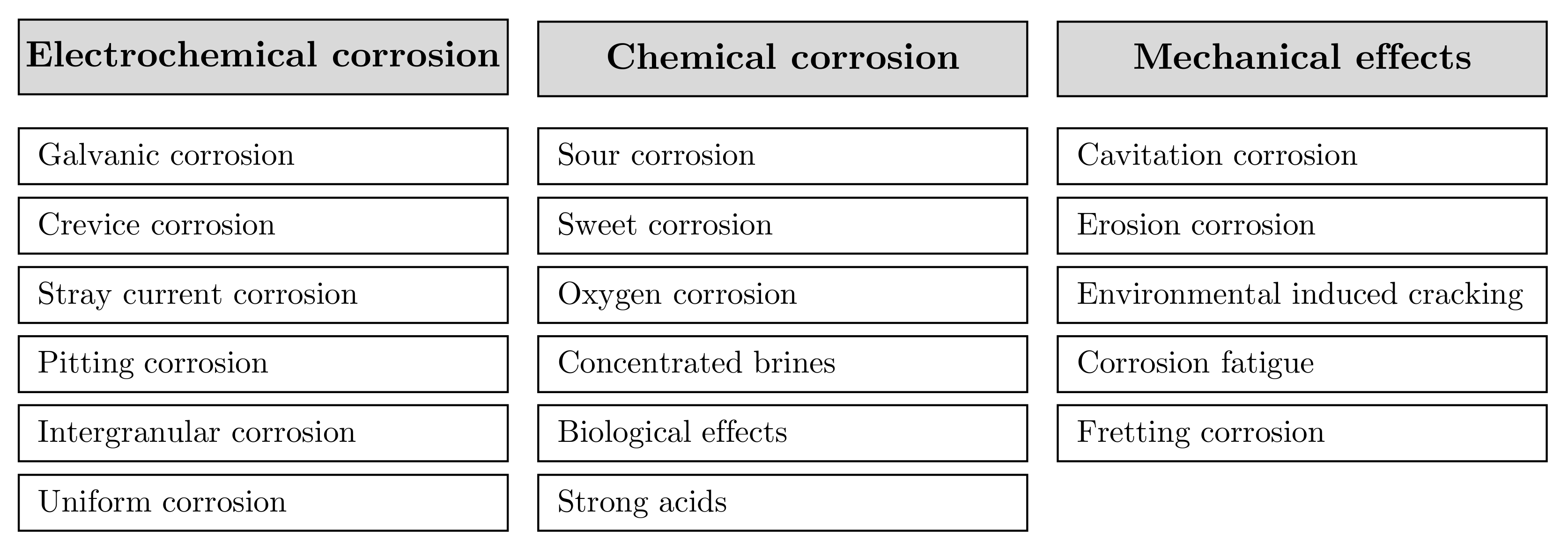
3. Injection Water Characteristics and Formation Damage Mechanisms
3.1. Oil Content
3.2. Total Suspended Solids
Thus, TSS and TDS are defined as follows:Total solids—The material left in a sample vessel after evaporation and subsequent oven drying at a defined temperature. Total solids include both total suspended and total dissolved solids, which are physically separated via filtration whether a solids particle is filtered into the “suspended” or “dissolved” portion principally depends on a filter’s thickness, area, pore size, porosity, and type of holder, as well as the physical nature, particle size, and amount of solids being filtered.[64]
TSS—The portion of total solids in an aqueous sample retained on the filter. Note: Some clays and colloids will pass through a 2 µ filter.[64]
TDS—The portion of total solids in a water sample that passes through a filter with a nominal pore size of 2.0 µ under specified condition.[64]
3.3. Total Dissolved Solids
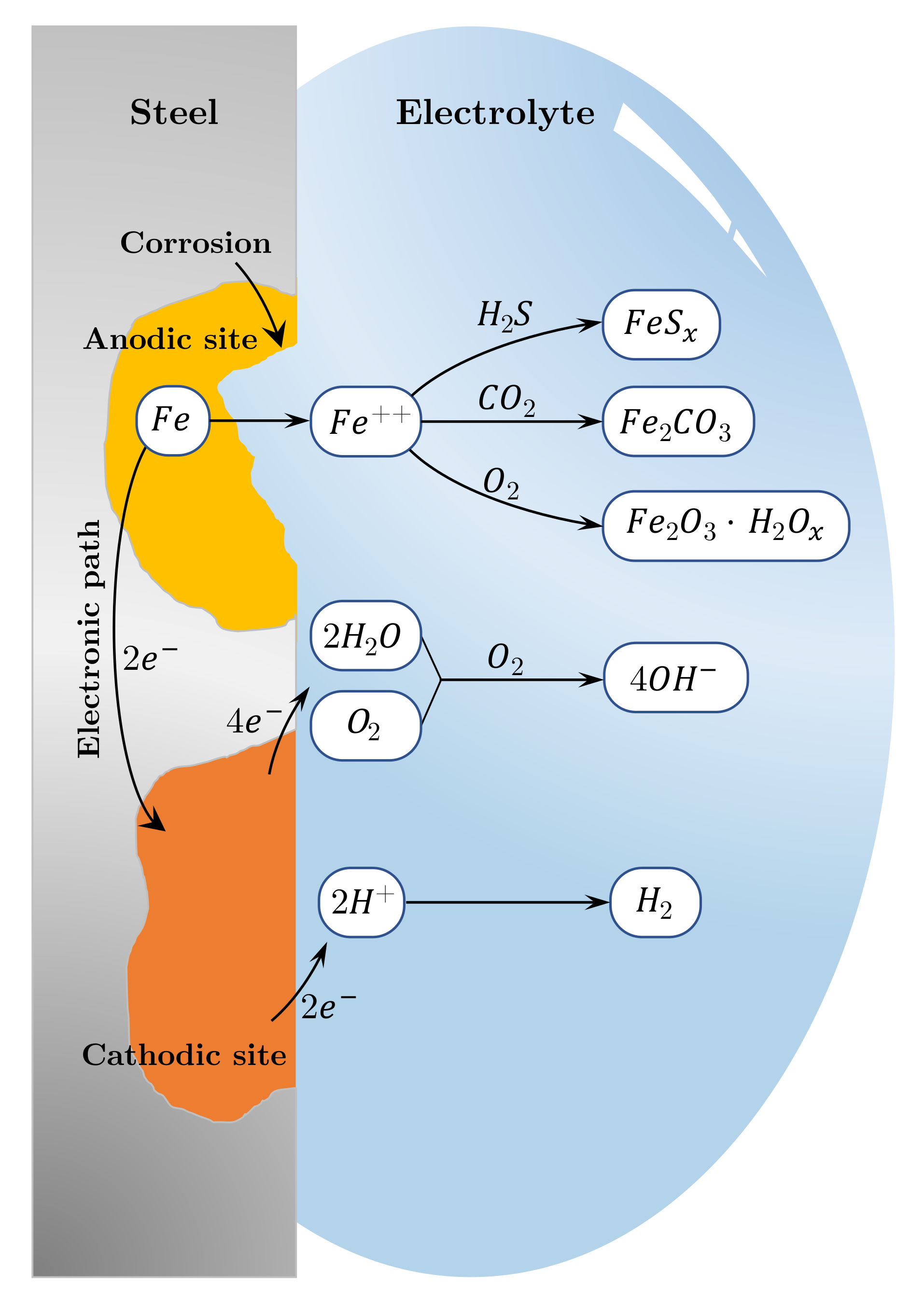
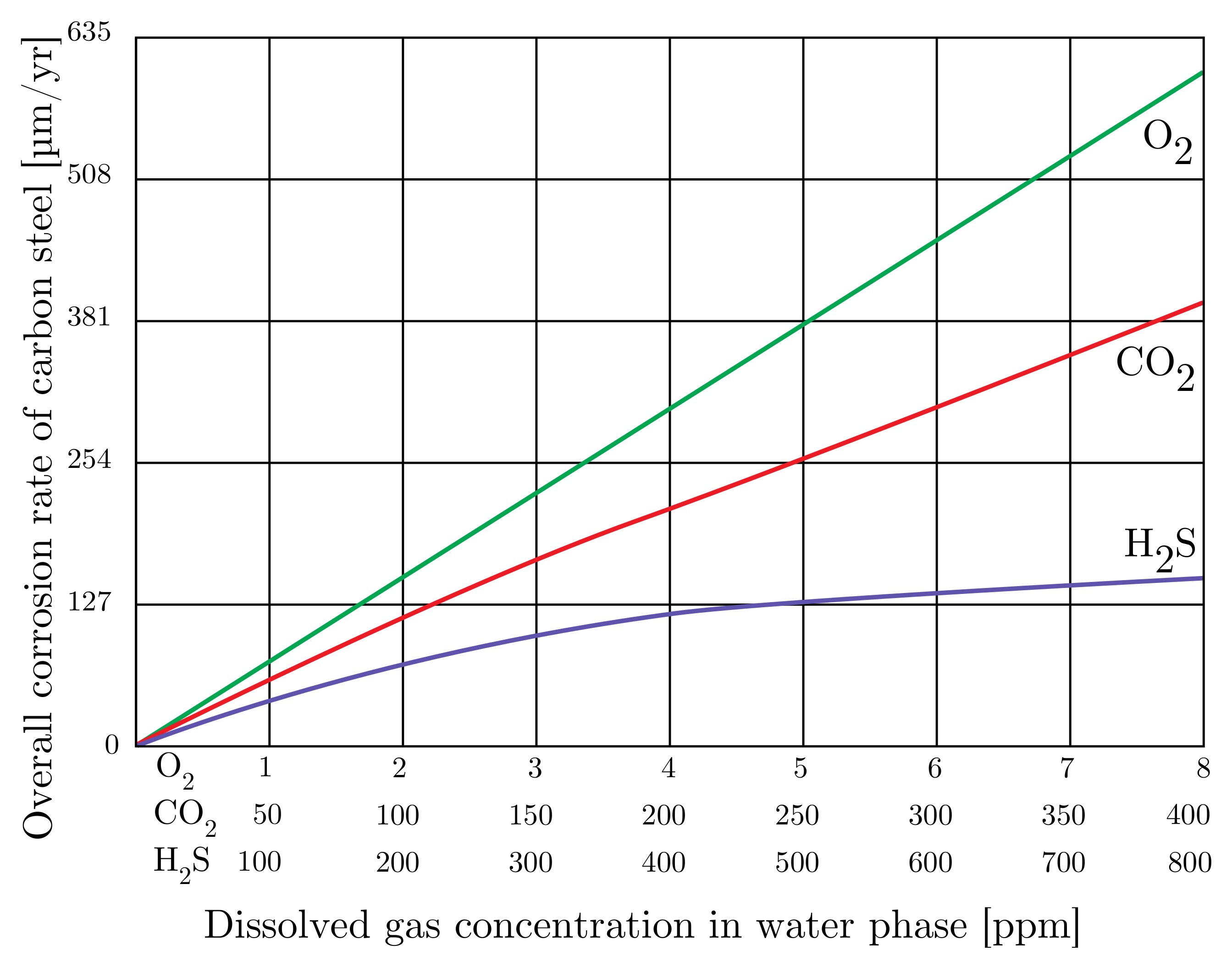
3.4. Dissolved Gases
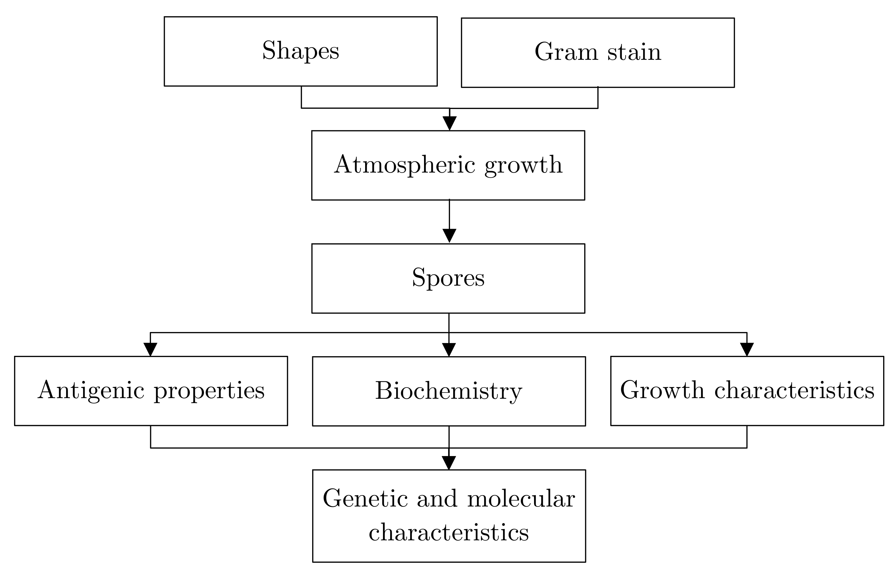
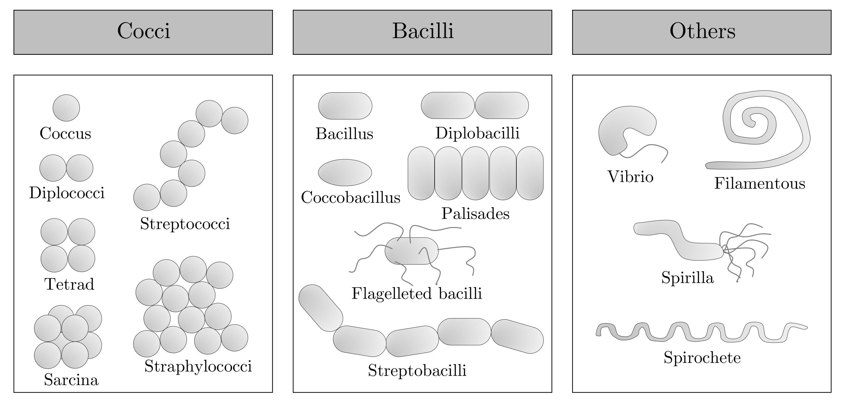
3.5. Bacterial Growth
- Obligate aerobic bacteria require O2 to multiply.
- Obligate anaerobic bacteria multiply in the absence of O2.
- Facultative anaerobic bacteria can multiply in both the present and absence of O2 due to its metabolism.
- Microaerophilic bacteria need the presence of O2. Though, at high concentrations of O2, they are poisoned.
- Aerotolerant microorganisms multiply in the absence of O2. Though they are not poisoned by O2 [117].
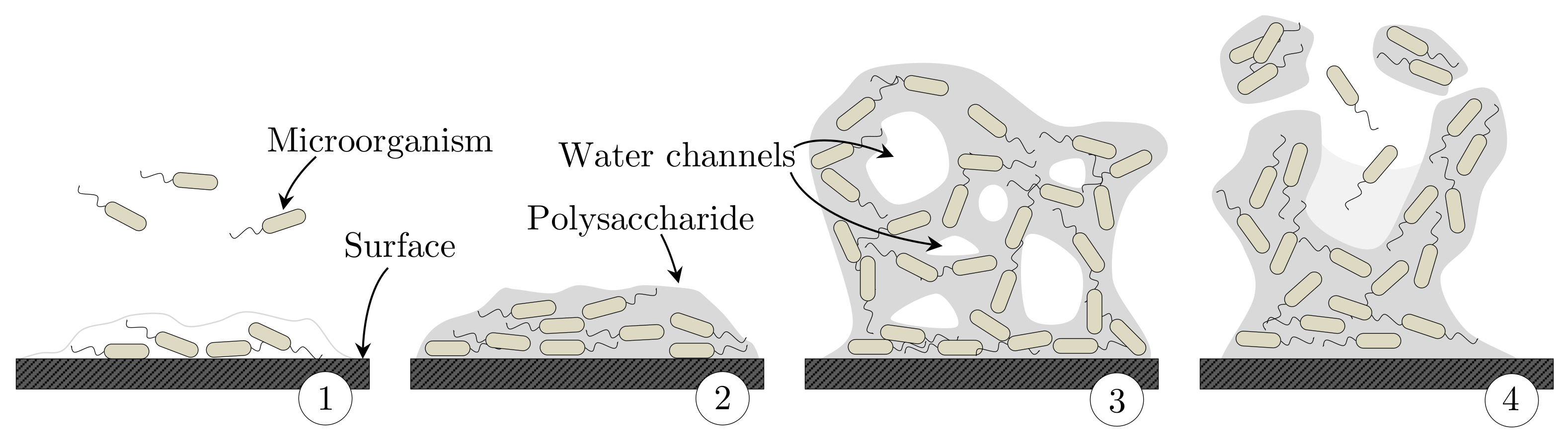
- Slime-forming bacteria (SFB)
- Metabolism: SFB covers a high amount of different bacteria [147]. SFB is a group of bacteria that is capable of producing a EPS, which acts as the foundation for the formation of biofilm. Many SFB fall within some of the other microbial groups [118,147]. Formation damage mechanisms: SFB has a indirectly influence of formation damage by promoting microbial growth inside the biofilm, attachment of other types of MIC, and development of in-situ ecosystem underneath a biofilm leads to formation of anodic and cathodic areas, promoting corrosion [148]. Type ex: Vibrio cholerae, as well as many other Vibrio spp., Clostridium spp., Flavobacterium spp., Bacillus spp., Pseudomonas spp., Pseudomonas, and Aerobacter [146,149,150].
- Sulphate-reducing bacteria/archaea (SRB/SRA)
- Metabolism: SRB are stated to be the most troublesome microbial group among MIC in the petroleum industry [151,152]. SRB and SRA, both of which primarily perform obligate anaerobic respiration, utilize sulfate (SO42−) as a terminal electron acceptor and generate H2S [120,137]. Formation damage mechanisms: Generation of H2S, which souring the process and their activity is primarily realized as a pitting attack on the metal surface [118,137]. Some studies even observed plugging of the injection well by corrosion deposit flocs due to the increase of H2S [152]. Types ex: Desulfovibrio, Desulfobacter, and Desulfotomaculum [149].
- Sulfate-oxidizing bacteria (SOB)
- Metabolism: SOB perform aerobic respiration. SOB can convert H2S, that is produced by SRB, to H2SO4 [120]. Formation damage mechanisms: The generation of sulfate-producing acids, such as H2SO4, are contributors to corrosion. If SRB and SOB are present these two type of groups almost always accompany each other, when the environmental conditions contains O2, it is suitable for the aerobic SOB, and vice versa [137,150,153]. Type ex: Thiobacillus spp., Paracoccus, Xanthobacter, Alcaligens, and Pseudomonas [149].
- Iron-reducing Bacteria (IRB)
- Metabolism: Most of the IRB are facultative anaerobes. IRB influences corrosion by reducing insoluble Fe3+ oxide layer to soluble Fe3+, or they replace the metal film on the pipeline surface with less stable metal film [137,146,154]. Formation damage mechanisms: Exposes the metal beneath corrosion deposits (Fe2O3) protective layer to a corrosive environment. IRB also makes the environment more suitable for SRB in a mixed population of microorganisms in the biofilm, as IRB consume the O2, and the SRB can thereby live under anaerobic conditions [137]. Type ex: Shewanella and Pseudomonas spp. [146,153].
- Iron/Manganese Oxidizing Bacteria (IOB)
- Metabolism: IOB form oxide and hydroxide mineral deposits that cover the metal surface and provide O2 depleted zones where anaerobe microorganisms can propagate [153,154]. Formation damage mechanisms: Promote corrosion reactions by the deposition on the metal surface, which decrease or damage the the protective oxide films covered on the surface [118,146]. Type ex: Gallionella, Leptothrix, Siderocapsa, Sphaerotilus, Crenothrix and Clonothrix [118,146,149,153].
- Acid-producing bacteria (APB)
- Metabolism: APB can produce large amounts of acids as by-products during their metabolism, which can decrease the pH in the biofilm into a very acidic environment [118,146]. Production of inorganic acids can be HNO3, H2SO3, H2SO4, HNO2, and H2CO3 [118]. For example, H2CO3 can then further disassociate into CO32− and CHO2− which can react with Fe resulting in the corrosion product FeCO3 [153]. Formation damage mechanisms: Produce acids that causing metals to dissolve and accelerate corrosion processes [153]. Type ex: Acetobacter, Gluconobacter, Pseudomonas, Thiobacillus, Thiothrix, and Beggiatoa spp. [118,153].
- Nitrate-Reducing Bacteria (NRB)
- Metabolism: NRB reduce N3− to N2. As previously described, nitrate is often injected into the process to mitigate souring caused by SRB, as NRB can outcompete SRB and thereby reduce H2S production. Studies proved that NRB efficiently oxidized the cathodic hydrogen from the metal, but unlike SRB cultures, they failed to stimulate the rate of corrosion [155]. Formation damage mechanisms: As previous described, corrosion caused by an NRB is more aggressive than SRB under strictly anaerobic conditions. Type ex: Arcobacter, Bacillus licheniformis, and Desulfovibrio.
3.6. Reflection
4. Injection Water Treatment Facility
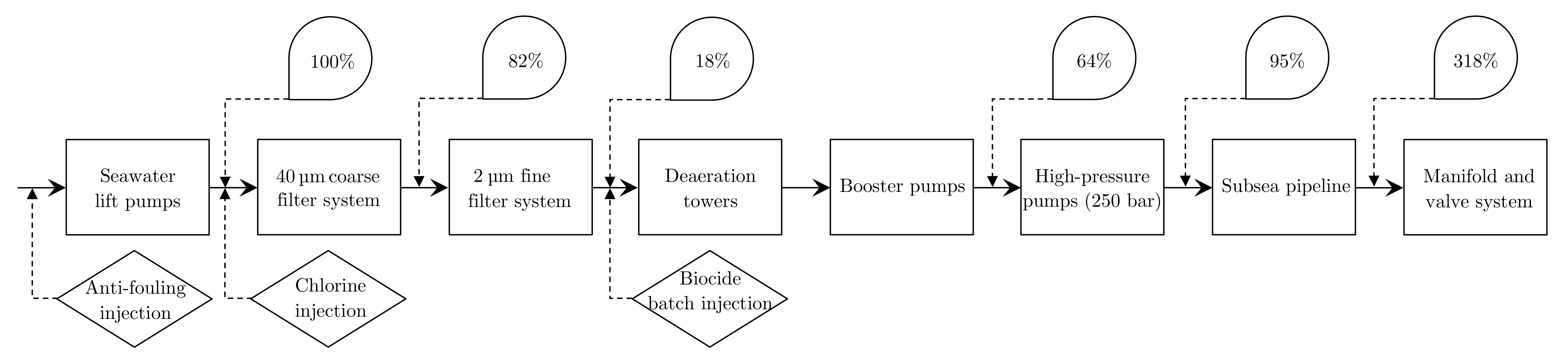
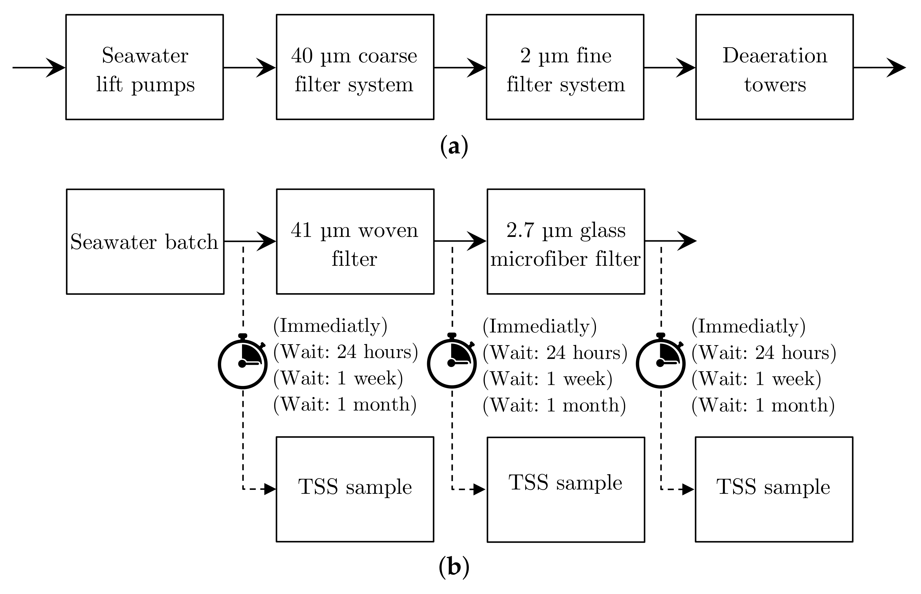
- Seawater Lifting Pumps: A few pumps lift seawater from the ocean to the platform level. These pumps are often controlled by a constant speed; 3–5 pumps are often required. As the seawater is untreated at this point, the dispersed and dissolved content are highly reactive, thus requiring the pump and piping at these early stages to be highly resilient. Therefore, an anti-fouling agent is added before the lifting pumps to eliminate fouling for this particular benchmarked IWT facility.
- Filtering: As solid particles are known to block pores in the reservoir, filters are utilized to remove sufficiently large solid particles. Chlorine is injected before the filter to protect the filters from biological fouling. At this time, there exist multiple solutions, but filtration systems might need improvements as the trend in oil and gas production is getting tighter, which involves injecting PW into the oil reservoir [160]. Some IWT solutions utilize a single-stage filter, where others use two-stage coarse and fine filters. Various types of filters are being used in the solution, such as cartridges, strainers, cyclones, membranes, and granular media types, where granular media types that define sand and nutshell filters are the most common [160]. As multiple of the same filter types are in use simultaneously in each train, it is of interest to divide the filter load equally among them as well as having an optimal filter cleaning procedure. The back-flushing cleaning procedure of the filters is commonly triggered by either exhausting a timer or after the delta pressure over the filter exceeds a limit [71]. It is also beneficial to balance the load between the coarse and fine filter states so that one stage is not redundant. As the continuous size distribution of the TSS is unknown, this load balance can be challenging to achieve [161].
- Deaeration: As O2 is unwanted in both the piping and reservoir, the concentration of O2 in the water is reduced by deaeration. A common deaeration method is by tray-type vacuum deaeration towers. The operating principle of the trays is to increase the surface area and reduce the travel length of O2. The deaeration towers’ performance is currently measured by analyzing samples of the IW before and after deaeration. However, there are various reliability issues of these measurements as the concentration of O2 in water should be low after deaeration. According to studies, the acceleration of corrosion occurs when the deaeration O2 content of the water is above 0.025 [99,100]. The concentration of O2 in the samples might change over time, from sample extraction to sample analysis, which causes errors when evaluating the performance [100].
- Injection Pump, Manifold, and Valve Systems: The booster pumps raise the pressure to 10–16 before the injection pumps raise the pressure to around 250–300 [158,159]. The IW is then either directly injected into the nearest wellheads or transported through a ∼10 long subsea pipeline, and some of the IW is even further transported ∼2 to another wellhead, where it enters the last part before injection into the reservoir [158,159].
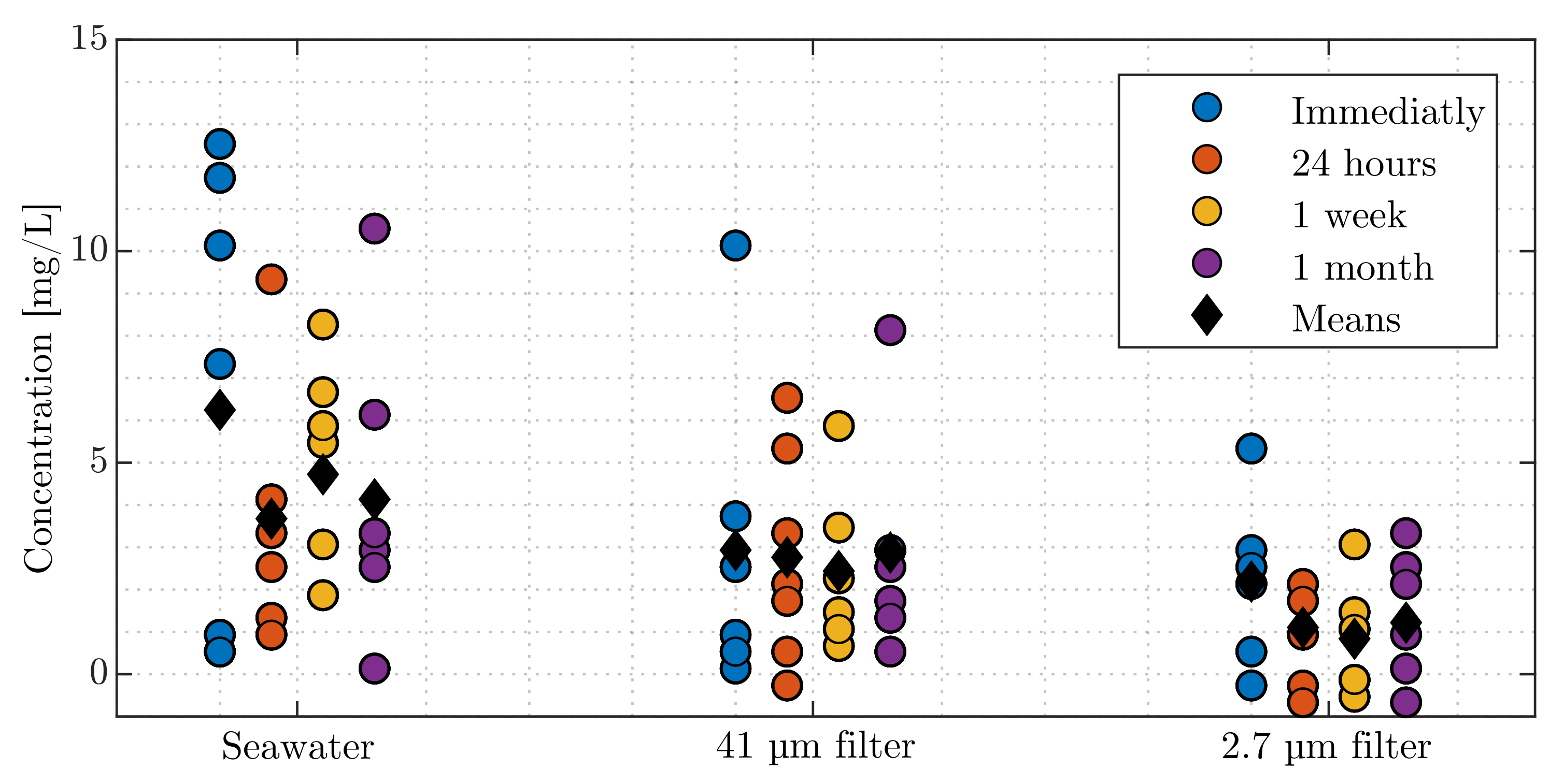
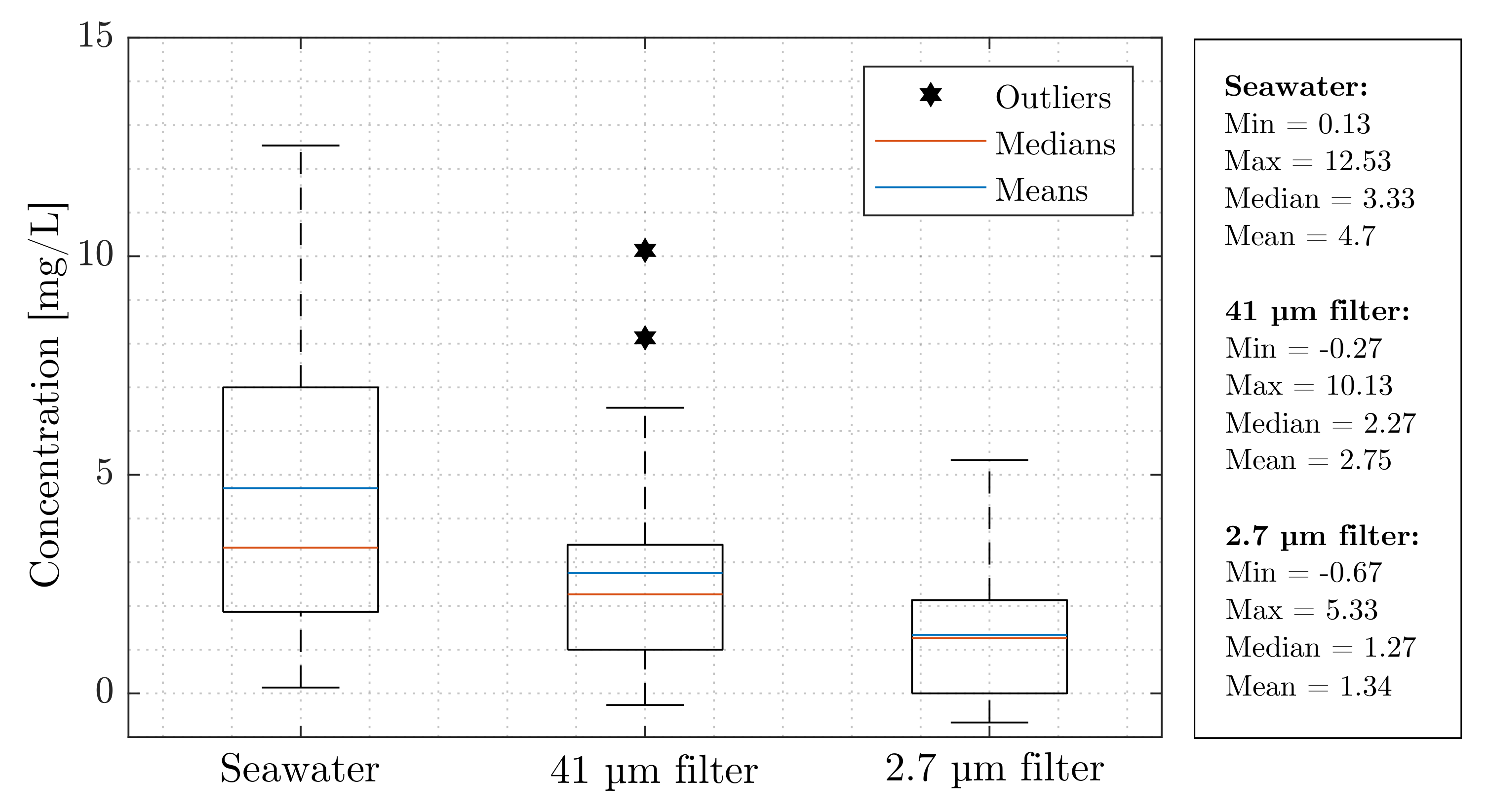
4.1. Total Suspended Solids Dried Weight Measurements
- 41 µ filter: Nylon filter—Sepctral/Mesh® Woven Filters—follows the U.S.A standard sieves ASTM specification E-11 for a mesh with a permissible variation of ±3 µ for a 41 µ filter [163];
- 2.7 µ filter: Glass Microfiber filters—WatmanTM 1823-047 Grade GF/D—Particle retention rating at 98% efficiency [164]; and
- 0.2 µ filter: Mixed Cellulose ester—Advantec® Membrane filters.
- Unfiltered seawater:
- 41 µ filter:
- 2.7 µ filter:
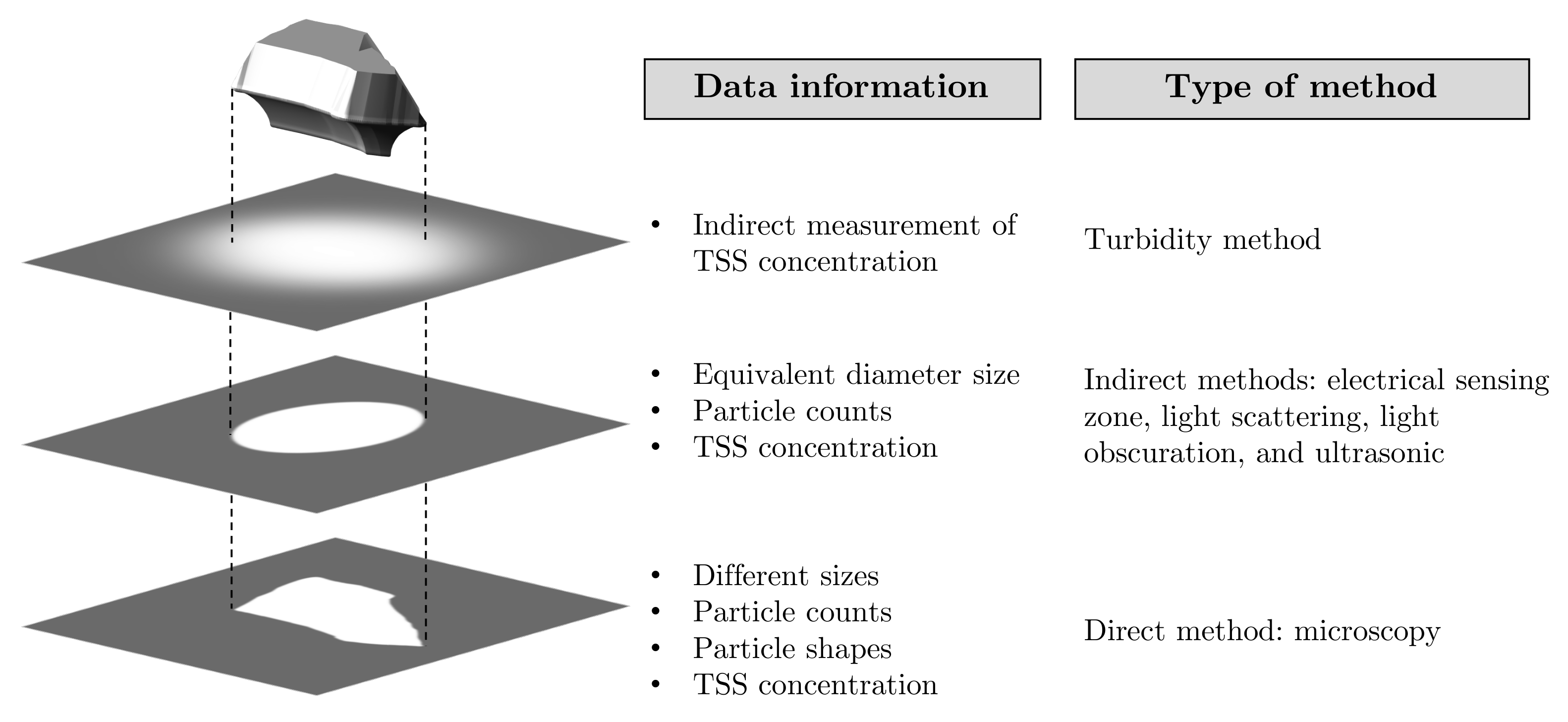
5. Online Monitoring Total Suspended Solids
5.1. Particle Size of Measurements
- linear dimension;
- projected area;
- surface area;
- volume;
- mass;
- settling rate; and
- the response of electrical, optical, or acoustical field.
5.2. Instrumentation
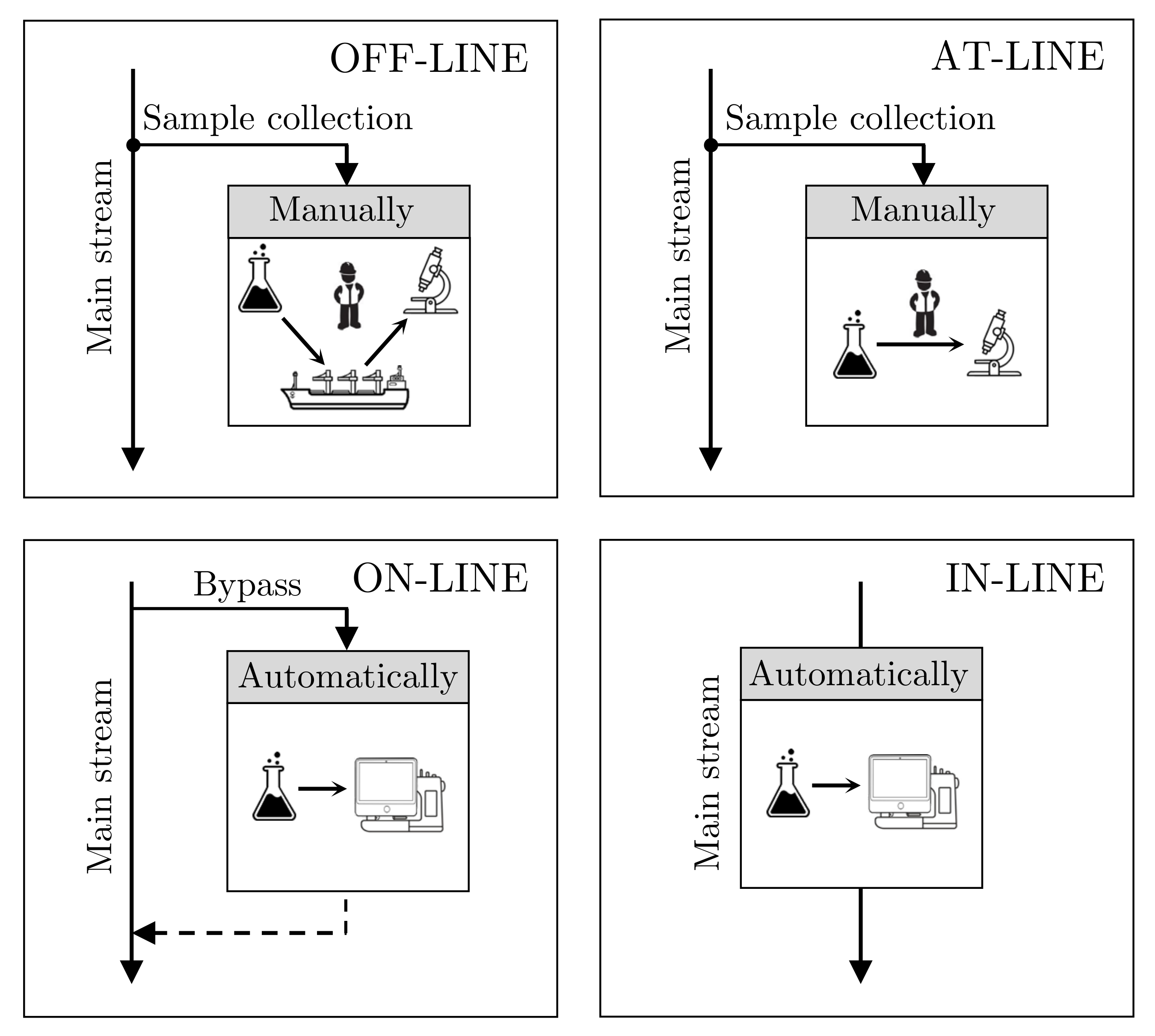
- Off-line analysis advantages in the manual examination of the sample are carried out by experts in laboratories. The sample preparation is adjusted to suit the particular method of analysis and types of quantities being examined. For off-line analysis offshore, the sample needs to be prepared (i.e., diluted, mixed, and preserved) to reduce changes under transportation, and a substantial number of samples are needed to verify the trueness of the measurement, which renders it a time-consuming process. Especially at offshore processes, it can take several days, if not weeks, between sampling collection and the results, obtained onshore. For this reason, feedback from the laboratories to the platform has a significantly longer reaction time, which is accentuated when a noteworthy deviation occurs due to faults of the production or, even worse, process damage.
- At-line analysis deviates from off-line analysis by carrying out the sampling analysis closer to the process. Like off-line analysis, at-line analysis is still a manual procedure that demands human resources compared to fully automated analysis procedures as on- and in-line analysis. The at-line location reduces the amount of preparation for transportation. Unlike off-line analysis, the closer proximity to the process also considerably reduces the reaction time, which could have a valuable effect on detecting adverse conditions earlier. Compared to off-line analysis, the disadvantage is that it may not be an ideal environment due to varying conditions, such as air humidity, temperature, and cleanliness.
- On-line analysis differs from the off-line and at-line methods as the sampling is automatic, which significantly reduces the reaction time of analyzing the quality of the IW. The automatic analysis guarantees the possibility of reacting promptly to any deviations from normal operation. To clarify, online monitors can be installed in both on-line and in-line configurations. TSS measurements have the potential to be used as feedback for improving process control. The disadvantage of on-line analysis, like off-line and at-line, is the risk of a bypassed maldistribution of the heterogeneous mainstream, which may not represent the true process quality. Manual sampling analysis is still necessary to verify the measurement quality of the TSS measurement equipment.
- In-line analysis and on-line analysis are closely related and share some advantages and disadvantages. An in-line analysis is done in-situ of the process stream directly. Thus, no misrepresentative sampling due to bypassing the flow happens nor disturbances in the process stream. However, the in-line analysis does have some disadvantages; the equipment must be robust within its procedure to prevent shutdowns from carrying out an inspection.
5.3. Particle Size Analysis Methods
- Turbidity method (Turbidimeters):
- Electrical Sensing Zone Method (Coulter Counter):
- Primary Coincidence: more than one particle in the sensing zone gives rise to two or more individual pulses which cannot be distinguished and are overestimated as one particle and lower the particle counts.
- Static Light Scattering method (Laser Diffraction):
- Light Obscuration Method:
- Ultrasonic Spectroscopy:
- Microscopy and Image Analysis:
5.4. Discrimination
or“…two-dimensional image cannot yield information on the three-dimensional particle unless the particle is either rotated or cut into slices during analysis.”
“…three-dimensional shape will at least demand information to be taken from three perpendicular planes.”
6. Conclusions
Author Contributions
Funding
Data Availability Statement
Acknowledgments
Conflicts of Interest
Abbreviations
| APB | acid-producing bacteria |
| API | American Petroleum Institute |
| ASTM | American Society for Testing and Materials |
| CDOM | colored dissolved organic matter |
| EIA | Energy Information Administration |
| EOR | enhanced oil recovery |
| EPS | extracellular polymeric substance |
| ESZ | electrical sensing zone |
| FFT | fast Fourier transform |
| GHG | greenhouse gases |
| H0 | null-hypotheses |
| HCI | human–computer interaction |
| IEA | International Energy Agency |
| IOB | iron/manganese-oxidizing bacteria |
| IRB | iron-reducing bacteria |
| ISO | International Organization for Standardization |
| IW | injection water |
| IWT | injection water treatment |
| MIC | microbially influenced corrosion |
| MDB | metal-depositing bacteria |
| MRB | metal-reducing bacteria |
| NGS | next-generation sequencing |
| NRB | nitrate-reducing bacteria |
| NTU | nephelometric turbidity units |
| OECD | Organisation for Economic Co-operation and Development |
| OIP | oil in place |
| OSPAR | Oslo and Paris Convention |
| ppm | parts per million |
| PSD | particle size distribution |
| PW | produced water |
| PWRI | produced water reinjection |
| SRB | sulfate-reducing bacteria |
| SFB | slime-forming bacteria |
| SSC | suspended sediment concentration |
| TDS | total dissolved solids |
| TPES | Total primary energy supply |
| TSS | total suspended solids |
| UV | ultraviolet |
References
- EIA. International Energy Outlook 2019; Technical Report; U.S. Energy Information Administration: Washington, DC, USA, 2019.
- IEA. Energy Access Outlook 2017; Technical Report; International Energy Agency: Paris, France, 2017. [Google Scholar]
- EIA. International Energy Outlook 2019: World Energy Projection System Plus; U.S. Energy Information Administration: Washington, DC, USA, 2019.
- SEI; IISD; ODI; Analytics Climate; CICERO; UNEP. The Production Gap: The Discrepancy between Countries’ Planned Fossil Fuel Production and Global Production Levels Consistent with Limiting Warming to 1.5 °C or 2 °C; Technical Report; The Production Gap: Geneva, Switzerland, 2019. [Google Scholar]
- IPIECA. Meeting Energy Needs: The Unique Role of Oil and Gas; Technical Report; The Global Oil and Gas Industry Association for Environmental and Social Issues: London, UK, 2014. [Google Scholar]
- Capodaglio, A.G.; Callegari, A. Online Monitoring Technologies For Drinking Water Systems Security. In Risk Management of Water Supply and Sanitation Systems; NATO Science for Peace and Security Series C: Environmental Security; Hlavinek, P., Popovska, C., Marsalek, J., Mahrikova, I., Kukharchyk, T., Eds.; Springer: Dordrecht, The Netherlands, 2009; pp. 153–179. [Google Scholar] [CrossRef]
- Blanchard, E. Oil in Water Monitoring is a Key to Production Separation. Offshore 2013, 73, 104–105. [Google Scholar]
- Maxwell, S. Implications of Re-Injection of Produced Water on Microbially Influenced Corrosion (MIC) in Offshore Water Injection Systems. In Proceedings of the CORROSION 2005, Houston, TX, USA, 3–7 April 2005; p. 9. [Google Scholar]
- OSPAR Commission. List of Decisions, Recommendations and Other Agreements Applicable within the Framework of the OSPAR Convention—Update 2018; Technical Report; OSPAR: London, UK, 2018. [Google Scholar]
- Severin Hansen, D.; Jespersen, S.; Bram, M.V.; Yang, Z. Uncertainty Analysis of Fluorescence-Based Oil-In-Water Monitors for Oil and Gas Produced Water. Sensors 2020, 20, 36. [Google Scholar] [CrossRef]
- Bavière, M. Basic Concepts in Enhanced Oil Recovery Processes, 1st ed.; Critical Reports on Applied Chemistry Volume 33; Elsevier: London, UK, 1991; pp. v–viii. [Google Scholar]
- Hartmann, D.J.; Beaumont, E.A. Predicting Reservoir System Quality and Performance. In Handbook of Petroleum Geology: Exploring for Oil and Gas Traps, 1st ed.; Beaumont, E.A., Foster, N.H., Eds.; The American Association of Petroleum Geologists: Tulsa, OK, USA, 1999; Volume 3, Chapter 9; p. 154. [Google Scholar] [CrossRef]
- Petroleum Council National; Enhanced Recovery Techniques; Committee on National Petroleum Council. Enhanced Oil Recovery, EOR: An Analysis of the Potential for Enhanced Oil Recovery from Known Fields in the United States, 1976 to 2000, 1st ed.; National Petroleum Council: Washington, DC, USA, 1976; p. 231. [Google Scholar]
- Marle, C.M. Oil entrapment and mobilization. In Basic Concepts in Enhanced Oil Recovery Processes, 1st ed.; Bavière, M., Ed.; Elsevier: Essex, UK, 1991; Volume 33, Chapter 1; pp. 3–39. [Google Scholar]
- British Petroleum. BP Statistical Review of World Energy June 2017; Technical Report; British Petroleum: London, UK, 2017. [Google Scholar]
- Ostroff, A. Injection Water Problems Identified By Laboratory Analysis. In Middle East Technical Conference and Exhibition; Society of Petroleum Engineers: Manama, Bahrain, 1981; pp. 523–526. [Google Scholar] [CrossRef]
- Carll, J.F. The Geology of the Oil Regions of Warren, Venango, Clarion, and Butler Counties; Including Surveys of the Garland and Panama conglomerates in Warren and Crawford, and in Chautauqua Co., N. Y., Descriptions of Oil Well Rig and Tools, and a Discussion of th, 1st ed.; Report of Progress; Harrisburg: Board of Commissioners for the Second Geological Survey: Washington, DC, USA, 1880; pp. 256–269. [Google Scholar]
- Simmons, A.C. Recent Developments in Water Flooding in the Bradford District. In Drilling and Production Practice; American Petroleum Institute: Amarillo, TX, USA, 1938; pp. 260–266. [Google Scholar]
- Cerini, W.F.; Battles, W.R.; Jones, P. Some Factors Influencing the Plugging Characteristics of an Oil-well Injection Water. Trans. AIME 1946, 165, 52–63. [Google Scholar] [CrossRef]
- Babson, E.; Sherborne, J.; Jones, P. An Experimental Water-flood in a California Oil Field. Trans. AIME 1944, 160, 25–33. [Google Scholar] [CrossRef]
- Ellenberger, A.R.; Holben, J.H. Flood Water Analyses and Interpretation. J. Pet. Technol. 1959, 11, 22–25. [Google Scholar] [CrossRef]
- Watkins, J.W.; Willett, F.R., Jr.; Arthur, C.E. Conditioning Water for Secondary-Recovery in Midcontinent Oil Fields; Technical Report; Bureau of Mines: Bartlesville, OK, USA; Washington, DC, USA, 1952.
- Safari, M. Effect of Different Water Injection Rate on Reservoir Performance: A Case Study of Azadegan Fractured Oil Reservoir. In Proceedings of the International Conference of Oil, Gas, Petrochemical and Power Plant, Tehran, Iran, 16 July 2012; Volume 1, p. 8. [Google Scholar]
- Yu, K.; Li, K.; Li, Q.; Li, K.; Yang, F. A method to calculate reasonable water injection rate for M oilfield. J. Pet. Explor. Prod. Technol. 2017, 7, 1003–1010. [Google Scholar] [CrossRef][Green Version]
- Bansal, K.; Caudle, D. A New Approach for Injection Water Quality. In Proceedings of the SPE Annual Technical Conference and Exhibition; Washington, DC, USA, 4–7 October 1992, pp. 383–396. [CrossRef]
- Patton, C.C. Water Quality Control and Its Importance in Waterflooding Operations. J. Pet. Technol. 1988, 40, 1123–1126. [Google Scholar] [CrossRef]
- Yari, M.; Mansouri, H.; Esmaili, H.; Alavi, S.A. A Study of Microbial Influenced Corrosion in Oil and Gas Industry. In International Conference of Oil, Gas, Petrochemical and Power Plant; Civilica: Tehran, Iran, 2012; Volume 1, p. 11. [Google Scholar] [CrossRef]
- Rochon, J.; Creusot, M.; Rivet, P.; Roque, C.; Renard, M. Water Quality for Water Injection Wells. In SPE Formation Damage Control Symposium; Society of Petroleum Engineers, Society of Petroleum Engineers: Lafayette, LA, USA, 1996; pp. 489–503. [Google Scholar] [CrossRef]
- Mitchell, R.W. The Forties Field Sea Water Injection System. J. Pet. Technol. 1978, 30, 877–884. [Google Scholar] [CrossRef]
- Mitchell, R.W.; Finch, E.M. Water Quality Aspects of North Sea Injection Water. J. Pet. Technol. 1981, 33, 1141–1152. [Google Scholar] [CrossRef]
- Prandle, D.; Hydes, D.J.; Jarvis, J.; McManus, J. The Seasonal Cycles of Temperature, Salinity, Nutrients and Suspended Sediment in the Southern North Sea in 1988 and 1989. Estuarine Coast. Shelf Sci. 1997, 45, 669–680. [Google Scholar] [CrossRef]
- Eisma, D.; Cadee, G.C.; Laane, R.W.P.M. Supply of Suspended Matter and Particulate and Dissolved Organic Carbon from the Rhine to the Coastal North Sea. Transp. Carbon Miner. Major World Rivers 1982, 52, 483–506. [Google Scholar]
- Aguirre-Gómez, R. Detection of total suspended sediments in the North Sea using AVHRR and ship data. Int. J. Remote. Sens. 2000, 21, 1583–1596. [Google Scholar] [CrossRef]
- Krumbein, W.C. Application of Logarithmic Moments to Size Frequency Distributions of Sediments. J. Sediment. Res. 1936, 6, 35–47. [Google Scholar] [CrossRef]
- Udden, J.A. The Mechanical Composition of Wind Deposits, 1st ed.; Number 1; Augustana College and Theological Seminary: Rock Island, IL, USA, 1898; p. 69. [Google Scholar]
- Wentworth, C.K. A Scale of Grade and Class Terms for Clastic Sediments. J. Geol. 1922, 30, 377–392. [Google Scholar] [CrossRef]
- Blott, S.J.; Pye, K. Particle Size Scales and Classification of Sediment Types Based on Particle Size Distributions: Review and Recommended Procedures. Sedimentology 2012, 59, 2071–2096. [Google Scholar] [CrossRef]
- Barkman, J.; Davidson, D. Measuring Water Quality and Predicting Well Impairment. J. Pet. Technol. 1972, 24, 865–873. [Google Scholar] [CrossRef]
- Patton, C.C. Injection-Water Quality. J. Pet. Technol. 1990, 42, 1238–1240. [Google Scholar] [CrossRef]
- Bennion, D.; Bennion, D.; Thomas, F.; Bietz, R. Injection Water Quality—A Key Factor to Successful Waterflooding. In Proceedings of the 45th Annual Technical Meeting, Calgary, AB, Canada, 12–15 June 1994; Volume 37, pp. 53–62. [Google Scholar] [CrossRef]
- Bennion, D.; Thomas, F.; Imer, D.; Ma, T.; Schulmeister, B. Water Quality Considerations Resulting in the Impaired Injectivity of Water Injection and Disposal Wells. J. Can. Pet. Technol. 2001, 40, 54–61. [Google Scholar] [CrossRef]
- Ogden, B.L. Water Technology: Understanding, Interpreting and Utilizing Water Analysis Data. In Southwestern Petroleum Short Course Conference 2008; Southwestern Petroleum Short Course: Lubbock, TX, USA, 2008; p. 12. [Google Scholar]
- Donham, J. Offshore Water Injection System: Problems and Solutions. In Proceedings of the Offshore Technology Conference, Houston, TX, USA, 6–9 May 1991; pp. 53–57. [Google Scholar] [CrossRef]
- Bader, M. Seawater versus produced water in oil-fields water injection operations. Desalination 2007, 208, 159–168. [Google Scholar] [CrossRef]
- Gao, C. Factors affecting particle retention in porous media. Emir. J. Eng. Res. 2007, 12, 7. [Google Scholar]
- Nielsen, B.L.; Nygaard, E.; Reffstrup, J.; Ter-Borch, N. Bjergarters Reservoiregenskaber; GEUS: Copenhagen, Denmark, 2019. [Google Scholar]
- Abramovitz, T. Geophysical imaging of porosity variations in the Danish North Sea chalk. Geol. Surv. Den. Greenl. Bull. 2008, 15, 17–20. [Google Scholar] [CrossRef]
- Jørgensen, L.N.; Andersen, P.M. Integrated Study of the Kraka Field. In Offshore Europe; Society of Petroleum Engineers: Aberdeen, China, 1991; pp. 461–474. [Google Scholar] [CrossRef]
- Hardman, R.F.P. Chalk reservoirs of the North Sea. Bull. Geol. Soc. Den. 1982, 30, 119–137. [Google Scholar]
- Torsaeter, O. An Experimental Study of Water Imbibition in Chalk From the Ekofisk Field. In SPE Enhanced Oil Recovery Symposium; Society of Petroleum Engineers: Tulsa, OK, USA, 1984; Volume 2, pp. 93–104. [Google Scholar] [CrossRef]
- Shutong, P.; Sharma, M. A Model for Predicting Injectivity Decline in Water-Injection Wells. SPE Form. Eval. 1997, 12, 194–201. [Google Scholar] [CrossRef]
- Eylander, J. Suspended Solids Specifications for Water Injection From Coreflood Tests. SPE Reserv. Eng. 1988, 3, 1287–1294. [Google Scholar] [CrossRef]
- Hansen, D.S.; Jespersen, S.; Bram, M.V.; Yang, Z. Human Machine Interface Prototyping and Application for Advanced Control of Offshore Topside Separation Processes. In Proceedings of the IECON 2018—44th Annual Conference of the IEEE Industrial Electronics Society, Washington, DC, USA, 21–23 October 2018; pp. 2341–2347. [Google Scholar] [CrossRef]
- Hansen, D.S.; Bram, M.V.; Yang, Z. Efficiency investigation of an offshore deoiling hydrocyclone using real-time fluorescence- and microscopy-based monitors. In Proceedings of the 2017 IEEE Conference on Control Technology and Applications (CCTA), Mauna Lani, HI, USA, 27–30 August 2017; pp. 1104–1109. [Google Scholar] [CrossRef]
- Yang, M. Measurement of Oil in Produced Water. In Produced Water, 1st ed.; Lee, K., Neff, J., Eds.; Springer: New York, NY, USA, 2011; Chapter 2; pp. 57–88. [Google Scholar] [CrossRef]
- Miløstyrelsen. Generel Tilladelse for Total E&P Danmark A/S (TOTAL) Til Anvendelse, Udledning OG Anden Bortskaffelse af Stoffer OG Materialer, Herunder Olie OG Kemikalier i Produktions- OG Injektionsvand Fra Produktionsenhederne Halfdan, Dan, Tyra og Gorm for perioden 1 January 2019–31 December 2020; Technical Report; Total E&P Danmark A/S: Copenhagen, Denmark, 2018. [Google Scholar]
- Danish Energy Agency. Production; Technical Report; Danish Energy Agency: Esbjerg, Denmark, 2016.
- Hansen, D.; Bram, M.; Durdevic, P.; Jespersen, S.; Yang, Z. Efficiency evaluation of offshore deoiling applications utilizing real-time oil-in-water monitors. In Proceedings of the Oceans 2017—Anchorage, Anchorage, AK, USA, 18–21 September 2017; p. 6. [Google Scholar]
- Danish Energy Agency. Yearly Production, Injection, Flare, Fuel and Export in SI Units 1972–2019; The Danish Energy Agency: Copenhagen, Denmark, 2020.
- OSPAR Commission. Produced Water Discharges from Offshore Oil and Gas Installations 2007–2012; OSPAR Commission: London, UK, 2014. [Google Scholar]
- Miløstyrelsen. Generel Tilladelse for Maersk Olie og Gas A/S (Maersk Olie) til Anvendelse, Udledning og Anden Bortskaffelse af Stoffer og Materialer, Herunder olie og Kemikalier i Produktions- og Injektionsvand fra Produktionsenhederne Halfdan, Dan, Tyra og Gorm for Perioden 1 January 2017–31 December 2018; Technical Report; Mærsk Olie og Gas A/S: Copenhagen, Denmark, 2016. [Google Scholar]
- OSPAR Commission. OSPAR Report on Discharges, Spills and Emissions from Offshore Oil and Gas Installations in 2014; Technical Report; OSPAR: London, UK, 2016. [Google Scholar]
- Kokal, S.; Al-Dawood, N.; Fontanilla, J.; Al-Ghamdi, A.; Nasr-El-Din, H.; Al-Rufaie, Y. Productivity Decline in Oil Wells Related to Asphaltene Precipitation and Emulsion Blocks. SPE Prod. Facil. 2003, 18, 247–256. [Google Scholar] [CrossRef]
- Baird, R.B.; Eaton, A.D.; Rice, E.W. Standard Methods for the Examination of Water and Wastewater, 23rd ed.; American Public Health Association, American Water Works Association, and Water Environment Federation: Washington, DC, USA, 2017; Chapter 2; pp. 66–82. [Google Scholar]
- Allhands, M.N. The Efficient Removal of Organic and Inorganic Suspended Solids—Old Problem, New Technology; Water Online Newsl: Horsham, PA, USA, 2016. [Google Scholar]
- Kennicutt, M.C. Water Quality of the Gulf of Mexico. In Habitats and Biota of the Gulf of Mexico: Before the Deepwater Horizon Oil Spill, 1st ed.; Ward, C.H., Ed.; Springer: New York, NY, USA, 2017; Volume 1, Chapter 2; pp. 55–164. [Google Scholar] [CrossRef]
- Boyd, C.E. Dissolved Solids. In Water Quality, 2nd ed.; Boyd, C.E., Ed.; Springer: Cham, Switzerland, 2015; Chapter 4; pp. 71–100. [Google Scholar] [CrossRef]
- Nasr-El-Din, H.; Al-Taq, A. Water Quality Requirements and Restoring the Injectivity of Waste Water Disposal Wells. In SPE Formation Damage Control Conference; Society of Petroleum Engineers: Lafayette, LA, USA, 1998; pp. 565–573. [Google Scholar] [CrossRef]
- Zheng, J.; Chen, B.; Thanyamanta, W.; Hawboldt, K.; Zhang, B.; Liu, B. Offshore produced water management: A review of current practice and challenges in harsh/Arctic environments. Mar. Pollut. Bull. 2016, 104, 7–19. [Google Scholar] [CrossRef]
- Coleman, J.; McLelland, W. Produced Water Re-Injection; How Clean is Clean? In SPE Formation Damage Control Symposium; Society of Petroleum Engineers: Lafayette, LA, USA, 1994; p. 5. [Google Scholar] [CrossRef]
- Jepsen, K.; Bram, M.; Pedersen, S.; Yang, Z. Membrane Fouling for Produced Water Treatment: A Review Study From a Process Control Perspective. Water 2018, 10, 847. [Google Scholar] [CrossRef]
- Owen, G.; Bandi, M.; Howell, J.A.; Churchouse, S.J. Economic assessment of membrane processes for water and waste water treatment. J. Membr. Sci. 1995, 102, 77–91. [Google Scholar] [CrossRef]
- van Oort, E.; van Velzen, J.; Leerlooijer, K. Impairment by Suspended Solids Invasion: Testing and Prediction. SPE Prod. Facil. 1993, 8, 178–184. [Google Scholar] [CrossRef]
- Kwon, D.Y.; Vigneswaran, S.; Fane, A.G.; Aim, R.B. Experimental determination of critical flux in cross-flow microfiltration. Sep. Purif. Technol. 2000, 19, 169–181. [Google Scholar] [CrossRef]
- Pautz, J.; Crocker, M.; Walton, C. Relating Water Quality and Formation Permeability to Loss of Injectivity. In SPE Production Operations Symposium; Society of Petroleum Engineers: Oklahoma City, OK, USA, 1989; pp. 565–576. [Google Scholar] [CrossRef]
- Abrams, A. Mud Design To Minimize Rock Impairment Due To Particle Invasion. J. Pet. Technol. 1977, 29, 586–592. [Google Scholar] [CrossRef]
- Wang, S.; Civan, F. Preventing Asphaltene Deposition in Oil Reservoirs by Early Water Injection. In SPE Production Operations Symposium; Society of Petroleum Engineers: Oklahoma City, OK, USA, 2005; p. 14. [Google Scholar] [CrossRef]
- Permadi, A.K.; Naser, M.A.; Mucharam, L.; Rachmat, S.; Kishita, A. Formation Damage and Permeability Impairment Associated with Chemical and Thermal Treatments: Future Challenges in EOR Applications. In The Contribution of Geosciences to Human Security, 1st ed.; Kyoto University GCOE Program of HSE; Institut Teknologi Bandung, Kyoto University: Berlin, Germany, 2012; Chapter 7; pp. 103–126. [Google Scholar]
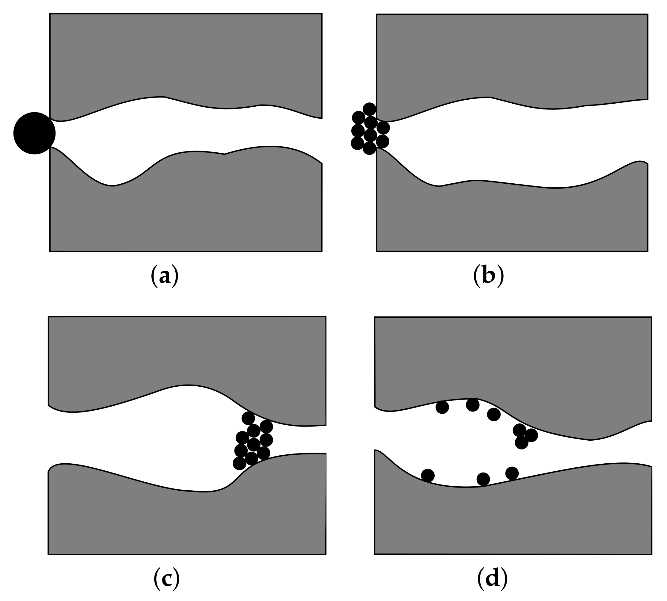
- Khilar, K.C.; Vaidya, R.; Fogler, H. Colloidally-induced fines release in porous media. J. Pet. Sci. Eng. 1990, 4, 213–221. [Google Scholar] [CrossRef]
- Bazin, B.; Esperanza, S.; Le Thiez, P. Control of Formation Damage by Modeling Water/Rock Interaction. In SPE Formation Damage Control Symposium; Society of Petroleum Engineers: Lafayette, LA, USA, 1994; pp. 249–258. [Google Scholar] [CrossRef]
- Shrestha, R.A.; Zhang, A.P.; Mateus, E.P.; Ribeiro, A.B.; Pamukcu, S. Electrokinetically Enabled De-swelling of Clay. In Electrokinetics Across Disciplines and Continents; Ribeiro, A.B., Mateus, E.P., Couto, N., Eds.; Springer: Cham, Switzerland, 2016; Chapter 3; pp. 43–56. [Google Scholar] [CrossRef]
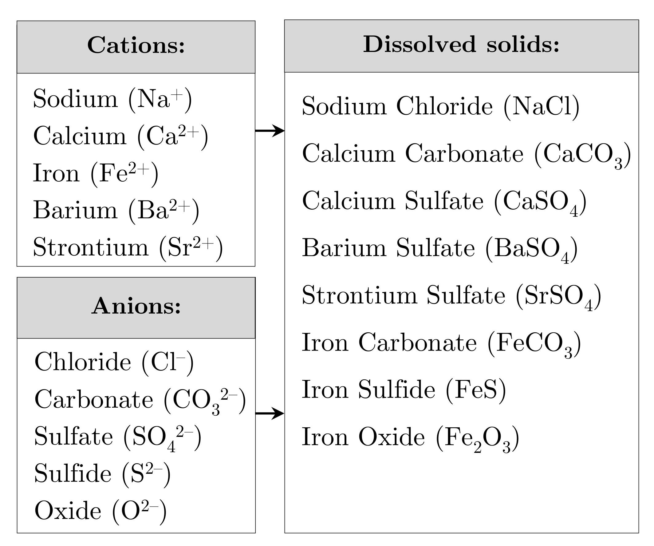
- Merdhah, A.B.B.M. The Study of Scale Formation in Oil Reservoir during Water Injection at High-Barium and High-Salinity Formation Water. Ph.D. Thesis, Universiti Teknologi Malaysia, Skudai, Malaysia, 2008. [Google Scholar]
- Amiri, M.; Moghadasi, J. Prediction the Amount of Barium Sulfate Scale Formation in Siri Oilfield using OLI ScaleChem Software. Asian J. Sci. Res. 2010, 3, 230–239. [Google Scholar] [CrossRef]
- Amiri, M.; Moghadasi, J.; Jamialahmadi, M. Prediction of Iron Carbonate Scale Formation in Iranian Oilfields at Different Mixing Ratio of Injection Water with Formation Water. Energy Sources Part Recover. Util. Environ. Eff. 2013, 35, 1256–1265. [Google Scholar] [CrossRef]
- Merdhah, A.B.B.; Yassin, A.A.M. Calcium and Strontium Sulfate Scale Formation Due to Incompatible Water. In Proceedings of the International Graduate Conference on Engineering and Science 2008, Johor, Malaysia, 23–24 December 2008; p. 9. [Google Scholar]
- Collins, I.R.; Jordan, M.M. Occurrence, Prediction, and Prevention of Zinc Sulfide Scale Within Gulf Coast and North Sea High-Temperature and High-Salinity Fields. SPE Prod. Facil. 2003, 18, 200–209. [Google Scholar] [CrossRef]
- Chester, R. Dissolved gases in sea water. In Marine Geochemistry, 1st ed.; Chester, R., Ed.; Springer: Dordrecht, The Netherlands, 1990; Chapter 8; pp. 233–271. [Google Scholar] [CrossRef]
- Brondel, D.; Montrouge, F.; Edwards, R.; Hayman, A.; Hill, D.; Mehta, S.; Semerad, T. Corrosion in the Oil Industry. Oilfield Rev. 1994, 6, 4–18. [Google Scholar]
- Ruschau, G.R.; Al-Anezi, A.M. Appendix S—Oil and Gas Exploration and Production. In Corrosion Cost and Preventive Strategies in the United States; Number FHWA-RD-01-156; Federal Highway Administration: McLean, VA, USA, 2001; Chapter Appendix S; p. 14. [Google Scholar]
- Popoola, L.; Grema, A.; Latinwo, G.; Gutti, B.; Balogun, A. Corrosion problems during oil and gas production and its mitigation. Int. J. Ind. Chem. 2013, 4, 15. [Google Scholar] [CrossRef]
- Koteeswaran, M. CO2 and H2S Corrosion in Oil Pipelines. Ph.D. Thesis, University of Stavanger, Stavanger, Norway, 2010. [Google Scholar]
- Heidersbach, R. Corrosion in Oil and Gas Production. In Microbiologically Influenced Corrosion in the Upstream Oil and Gas Industry, 1st ed.; Skovhus, T.L., Enning, D., Lee, J.S., Eds.; CRC Press: Boca Raton, FL, USA, 2017; Chapter 1; pp. 3–34. [Google Scholar] [CrossRef]
- Diaz, E.F.; Gonzalez-Rodriguez, J.G.; Martinez-Villafañe, A.; Gaona-Tiburcio, C. H2S corrosion inhibition of an ultra high strength pipeline by carboxyethyl-imidazoline. J. Appl. Electrochem. 2010, 40, 1633–1640. [Google Scholar] [CrossRef]
- Stansbury, E.E.; Buchanan, R.A. Fundamentals of Electrochemical Corrosion, 1st ed.; ASM International: Materials Park, OH, USA, 2000; p. 487. [Google Scholar]
- Norsworthy, R. Understanding corrosion in underground pipelines: Basic principles. In Underground Pipeline Corrosion, 1st ed.; Woodhead Publishing Series in Metals and Surface Engineering; Orazem, M.E., Ed.; Woodhead Publishing: Cambridge, UK, 2014; Chapter 1; pp. 3–34. [Google Scholar] [CrossRef]
- Jomdecha, C.; Prateepasen, A.; Kaewtrakulpong, P. Study on source location using an acoustic emission system for various corrosion types. NDT & E Int. 2007, 40, 584–593. [Google Scholar] [CrossRef]
- Landolt, D. Corrosion and Surface Treatment. In Electrochemistry; Feliu-Martinesz, J.M., Paya, V.C., Eds.; EOLSS Publishers: Oxford, UK, 2009; Chapter 6; pp. 240–271. [Google Scholar]
- American Water Works Association. Chemistry of Corrosion. In M27—External Corrosion Control for Infrastructure Sustainability, 3rd ed.; De Nileon, G.P., Gray, M.R., Armstrong, C., Beach, M., Eds.; Manual of Water Supply Practices, American Water Works Association: Denver, CO, USA, 2014; Chapter 2; pp. 7–24. [Google Scholar]
- Byars, H.; Gallop, B. Injection Water + Oxygen = Corrosion and/or Well Plugging Solids. In SPE Symposium on Handling of Oilfield Water; Society of Petroleum Engineers: Los Angeles, CA, USA, 1972; pp. 96–102. [Google Scholar] [CrossRef]
- Durdevic, P.; Raju, C.S.; Yang, Z. Potential for Real-Time Monitoring and Control of Dissolved Oxygen in the Injection Water Treatment Process. IFAC PapersOnLine 2018, 51, 170–177. [Google Scholar] [CrossRef]
- Zardynezhad, S. Consider Key Factors in Pipeline Wall Thickness Calculation and Selection; Gas Process. & LNG: Louis, MO, USA, 2015. [Google Scholar]
- Beavers, J.A.; Thompson, N.G. External corrosion of oil and natural gas pipelines. In ASM handbook Volume 13C: Corrosion: Environments and Industries, 1st ed.; ASM Handbook; Cramer, S.D., Bernard, S., Covino, J., Eds.; ASM International: Materials Park, OH, USA, 2006; Chapter 100; pp. 1015–1025. [Google Scholar] [CrossRef]
- Shirazi, S.A.; Mclaury, B.S.; Shadley, J.R.; Roberts, K.P.; Rybicki, E.F.; Rincon, H.E.; Hassani, S.; Al-Mutahar, F.M.; Al-Aithan, G.H. Erosion–Corrosion in Oil and Gas Pipelines. In Oil and Gas Pipelines: Integrity and Safety Handbook, 1st ed.; Revie, R.W., Ed.; John Wiley & Sons, Inc.: Hoboken, NJ, USA, 2015; Chapter 28; pp. 399–422. [Google Scholar] [CrossRef]
- Sastri, V.S. Corrosion Causes. In Challenges in Corrosion: Costs, Causes, Consequences, and Control, 1st ed.; Revie, R.W., Ed.; Wiley Series in Corrosion; John Wiley & Sons: Hoboken, NJ, USA, 2015; Chapter 3; pp. 127–204. [Google Scholar] [CrossRef]
- Farshad, F.F.; Choate, L.C.; Winters, R.H.; Garber, J.D. Pipeline Optimization—A Surface Roughness Approach; Technical Report; University of Louisiana: Lafayette, LA, USA, 2017. [Google Scholar]
- Skovhus, T.L.; Enning, D.; Lee, J.S. Microbiologically Influenced Corrosion in the Upstream Oil and Gas Industry, 1st ed.; CRC Press: Boca Raton, FL, USA, 2017; pp. v–xxvi. [Google Scholar] [CrossRef]
- Ren, H.; Xiong, S.; Gao, G.; Song, Y.; Cao, G.; Zhao, L.; Zhang, X. Bacteria in the injection water differently impacts the bacterial communities of production wells in high-temperature petroleum reservoirs. Front. Microbiol. 2015, 6, 8. [Google Scholar] [CrossRef]
- Ismail, W.A.; Van Hamme, J.D.; Kilbane, J.J.; Gu, J.D. Editorial: Petroleum Microbial Biotechnology: Challenges and Prospects. Front. Microbiol. 2017, 8, 4. [Google Scholar] [CrossRef]
- Bouchard, R.P. Is a Virus a Living Creature? Medium: San Francisco, CA, USA, 2017. [Google Scholar]
- Wang, I.; Burckhardt, C.J.; Yakimovich, A.; Greber, U.F. Imaging, Tracking and Computational Analyses of Virus Entry and Egress with the Cytoskeleton. Viruses 2018, 10, 29. [Google Scholar] [CrossRef] [PubMed]
- Cole, L.A. Evolutionary History of Planet Earth. In Biology of Life: Biochemistry, Physiology and Philosophy, 1st ed.; Tenney, S., Ed.; Academic Press: Cambridge, MA, USA, 2016; Chapter 6; pp. 37–43. [Google Scholar] [CrossRef]
- Schloss, P.D.; Handelsman, J. Status of the Microbial Census. Microbiol. Mol. Biol. Rev. 2004, 68, 686–691. [Google Scholar] [CrossRef]
- Whitman, W.B.; Coleman, D.C.; Wiebe, W.J. Prokaryotes: The unseen majority. Proc. Natl. Acad. Sci. USA 1998, 95, 6578–6583. [Google Scholar] [CrossRef] [PubMed]
- Baron, E.J. Classification. In Medical Microbiology, 4th ed.; Baron, S., Ed.; University of Texas Medical Branch: Galveston, TX, USA, 1996; Chapter 3. [Google Scholar]
- Gillespie, S.H.; Bamford, K.B. Structure and Classification of Bacteria. In Medical Microbiology and Infection at a Glance, 4th ed.; Wiley-Blackwell: Hoboken, NJ, USA, 2012; Chapter 1; pp. 8–9. [Google Scholar]
- Barnes-Svarney, P.; Svarney, T.E. The Handy Biology Answer Book, 2nd ed.; Visible Ink Press: Canton, MI, USA, 2015; pp. 1–496. [Google Scholar]
- Barer, M.R. Bacterial growth, physiology and death. In Medical Microbiology: A Guide to Microbial Infections: Pathogenesis, Immunity, Laboratory Diagnosis and Control, 18th ed.; Greenwood, D., Barer, M.R., Slack, R.C.B., Irving, W.L., Eds.; Churchill Livingstone: London, UK, 2012; Chapter 4; pp. 39–53. [Google Scholar] [CrossRef]
- Beech, I.; Flemming, H.C.; Mollica, A.; Scotto, V. Simple Methods for the Investigation of of the Role of Biofilms in Corrosion. Technical Report; European Commission Federation of Corrosion: Stockholm, Sweden, 2000. [Google Scholar]
- MacLeod, R.A. The Question of the Existence of Specific Marine Bacteria. Bacteriol. Rev. 1965, 29, 9–24. [Google Scholar] [CrossRef] [PubMed]
- Little, B.; Wagner, P.; Mansfeld, F. An Overview of Microbiologically Influenced Corrosion. Electrochim. Acta 1992, 37, 2185–2194. [Google Scholar] [CrossRef]
- Little, B.J.; Lee, J.S. Microbiologically Influenced Corrosion, 1st ed.; John Wiley & Sons, Inc.: Hoboken, NJ, USA, 2007; p. 280. [Google Scholar] [CrossRef]
- Heitz, E.; Flemming, H.C.; Sand, W. Microbially Influenced Corrosion of Materials: Scientific and Engineering Aspects, 1st ed.; Springer: Berlin/Heidelberg, Germany, 1996; p. 475. [Google Scholar]
- Fischer, D.; Canalizo-Hernandez, M.; Kumar, A. Effects of Reservoir Souring on Materials Performance. In Microbiologically Influenced Corrosion in the Upstream Oil and Gas Industry, 1st ed.; Skovhus, T.L., Enning, D., Lee, J.S., Eds.; CRC Press: Boca Raton, FL, USA, 2017; Chapter 6; pp. 111–137. [Google Scholar] [CrossRef]
- Mittelman, M.W. Bacterial Biofilms and Bifouling: Translational Research in Marine Biotechnology. In Opportunities for Environmental Applications of Marine Biotechnology; Vaupel, S., Ed.; National Academies Press: Washington, DC, USA, 2000; Chapter 2; pp. 3–7. [Google Scholar] [CrossRef]
- Komlenic, R. Rethinking the causes of membrane biofouling. Filtr. Sep. 2010, 47, 26–28. [Google Scholar] [CrossRef]
- Donlan, R.M. Biofilms: Microbial Life on Surfaces. Emerg. Infect. Dis. 2002, 8, 881–890. [Google Scholar] [CrossRef] [PubMed]
- Vasudevan, R. Biofilms: Microbial Cities of Scientific Significance. J. Microbiol. Exp. 2014, 1, 1–16. [Google Scholar] [CrossRef]
- Nguyen, T.; Roddick, F.; Fan, L. Biofouling of Water Treatment Membranes: A Review of the Underlying Causes, Monitoring Techniques and Control Measures. Membranes 2012, 2, 804–840. [Google Scholar] [CrossRef] [PubMed]
- Sauer, K.; Camper, A.K.; Ehrlich, G.D.; Costerton, J.W.; Davies, D.G. Pseudomonas aeruginosa displays multiple phenotypes during development as a biofilm. J. Bacteriol. 2002, 184, 1140–1154. [Google Scholar] [CrossRef]
- Macià, M.D.; Rojo-Molinero, E.; Oliver, A. Antimicrobial susceptibility testing in biofilm-growing bacteria. Clin. Microbiol. Infect. Off. Publ. Eur. Soc. Clin. Microbiol. Infect. Dis. 2014, 20, 981–990. [Google Scholar] [CrossRef]
- Mah, T.F.C.; O’Toole, G.A. Mechanisms of biofilm resistance to antimicrobial agents. Trends Microbiol. 2001, 9, 34–39. [Google Scholar] [CrossRef]
- Hall-Stoodley, L.; Costerton, J.W.; Stoodley, P. Bacterial biofilms: From the Natural environment to infectious diseases. Nat. Rev. Microbiol. 2004, 2, 95–108. [Google Scholar] [CrossRef]
- Tidwell, T.J.; Keasler, V.; Paula, R.D. How Production Chemicals Can Influence Microbial Susceptibility to Biocides and Impact Mitigation Strategies. In Microbiologically Influenced Corrosion in the Upstream Oil and Gas Industry, 1st ed.; Skovhus, T.L., Enning, D., Lee, J.S., Eds.; CRC Press: Boca Raton, FL, USA, 2017; Chapter 19; pp. 379–392. [Google Scholar] [CrossRef]
- Little, B.; Lee, J.; Ray, R. New Developments in Mitigation of Microbiologically Influenced Corrosion; Technical Report; Naval Research Laboratory Oceanography Division Stennis Space Center: Fort Belvoir, VA, USA, 2007. [Google Scholar]
- Turkiewicz, A.; Brzeszcz, J.; Kapusta, P. The application of biocides in the oil and gas industry. Nafta-Gaz 2013, 69, 103–111. [Google Scholar] [CrossRef]
- Laura Machuca Suarez. Microbiologically Induced Corrosion Associated with the Wet Storage of Subsea Pipelines (Wet Parking). In Microbiologically Influenced Corrosion in the Upstream Oil and Gas Industry, 1st ed.; Skovhus, T.L., Enning, D., Lee, J.S., Eds.; CRC Press: Boca Raton, FL, USA, 2017; Chapter 18; pp. 361–378. [Google Scholar] [CrossRef]
- Javaherdashti, R. Microbiologically Influenced Corrosion, 2nd ed.; Engineering Materials and Processes; Springer: London, UK, 2008; p. 216. [Google Scholar] [CrossRef]
- Sandbeck, K.; Hitzman, D. Biocompetitive Exclusion Technology: A Field System to Control Reservoir Souring and Increasing Production. In Proceedings of the Fifth International Conference on Microbial Enhanced Oil Recovery and Related Biotechnology for Solving Environment Problems, Dallas, TX, USA, 11–14 September 1995; pp. 311–319. [Google Scholar]
- Schwermer, C.U.; Lavik, G.; Abed, R.M.M.; Dunsmore, B.; Ferdelman, T.G.; Stoodley, P.; Gieseke, A.; de Beer, D. Impact of Nitrate on the Structure and Function of Bacterial Biofilm Communities in Pipelines Used for Injection of Seawater into Oil Fields. Appl. Environ. Microbiol. 2008, 74, 2841–2851. [Google Scholar] [CrossRef]
- Hubert, C.; Voordouw, G.; Arensdorf, J.; Jenneman, G.E. Control of souring through a novel class of bacteria that oxidize sulfide as well as oil organics with nitrate. In Proceedings of the CORROSION/2006, NACE International, San Diego, CA, USA, 12–16 March 2006; p. 10. [Google Scholar]
- Xu, D. Microbiologically Influenced Corrosion (MIC) Mechanisms and Mitigation. Ph.D. Thesis, Ohio University, Athens, OH, USA, 2013. [Google Scholar]
- Jones, S.E.; Lennon, J.T. Dormancy contributes to the maintenance of microbial diversity. Proc. Natl. Acad. Sci. USA 2010, 107, 5881–5886. [Google Scholar] [CrossRef]
- Lewis, K. Persister cells, dormancy and infectious disease. Nat. Rev. Microbiol. 2007, 5, 48–56. [Google Scholar] [CrossRef]
- El-Baky, R. The Future Challenges Facing Antimicrobial Therapy: Resistance and Persistence. Am. J. Microbiol. Res. 2016, 4, 15. [Google Scholar] [CrossRef]
- Stewart, E.J. Growing Unculturable Bacteria. J. Bacteriol. 2012, 194, 4151–4160. [Google Scholar] [CrossRef] [PubMed]
- Hu, A. Investigation of Sulfate-Reducing Bacteria Growth Behavior for the Mitigation of Microbiologically Influenced Corrosion (MIC). Ph.D. Thesis, Ohio University, Athens, OH, USA, 2004. [Google Scholar]
- Klai, N.; Yan, S.; Tyagi, R.D.; Surampalli, R.Y. EPS producing microorganisms from municipal wastewater activated sludge. J. Pet. Environ. Biotechnol. 2016, 7, 13. [Google Scholar] [CrossRef]
- Raulio, M. Ultrastructure of Biofilms Formed by Bacteria From Industrial Processes. Ph.D. Thesis, University of Helsinki, Helsinki, Finland, 2010. [Google Scholar]
- Natarajan, K. Biofouling and Microbially Influenced Corrosion of Stainless Steels. Adv. Mater. Res. 2013, 794, 539–551. [Google Scholar] [CrossRef]
- Borenstein, S.W. Microbiology. In Microbiologically Influenced Corrosion Handbook, 1st ed.; Woodhead Publishing: Cambridge, UK, 1994; Chapter 2; pp. 8–49. [Google Scholar] [CrossRef]
- Coetser, S.E.; Cloete, T.E. Biofouling and Biocorrosion in Industrial Water Systems. Crit. Rev. Microbiol. 2005, 31, 213–232. [Google Scholar] [CrossRef]
- Okabe, S.; Jones, W.L.; Lee, W.; Characklis, W.G. Anaerobic SRB Biofilms in Industrial Waters Systems: A process Analysis. In Biofouling and Biocorrosion in Industrial Water Systems, 1st ed.; Geesey, G.G., Lewandowski, Z., Flemming, H.C., Eds.; CRC Press: Boca Raton, FL, USA, 1994; Chapter 12; pp. 189–204. [Google Scholar]
- Sharma, M.; Voordouw, G. MIC Detection and Assessment A Holistic Approach. In Microbiologically Influenced Corrosion in the Upstream Oil and Gas Industry, 1st ed.; Skovhus, T.L., Enning, D., Lee, J.S., Eds.; CRC Press: Boca Raton, FL, USA, 2017; Chapter 9; pp. 177–212. [Google Scholar] [CrossRef]
- Papavinasam, S. Mechanisms. In Corrosion Control in the Oil and Gas Industry, 1st ed.; Gulf Professional Publishing: Houston, TX, USA, 2014; Chapter 5; pp. 249–300. [Google Scholar] [CrossRef]
- Cord-Ruwisch, R. MIC in Hydrocarbon Transportation Systems. In Corrosion Australasia; Australasian Corrosion Association: Perth, WA, USA, 1995; pp. 8–12. [Google Scholar]
- Zhang, J. RPSEA Subsea Produced Water Discharge Sensor Lab Test Results and Recommendations Final Report; Technical Report 3; Cleariew Subsea LLC: Houston, TX, USA, 2016. [Google Scholar]
- Maersk Oil. Maersk Oil ESIA-16 Non-Technical Summary—ESIS Dan; Technical Report; Maersk Oil: Esbjerg, Denmark, 2015. [Google Scholar]
- Larsen, J.; Rod, M.H.; Zwolle, S. Prevention of Reservoir Souring in the Halfdan Field by Nitrate Injection. In Proceedings of the Corrosion 2004, New Orleans, LA, USA, 28 March–1 April 2004; NACE International. p. 9. [Google Scholar]
- Thomsen, U.S.; Markfoged, R.; Meng, R.; Choong, L. Quantification of Microbiologically Influenced Corrosion in Injection Water Pipelines. In Proceedings of the Corrosion 2017, New Orleans, LA, USA, 26–30 March 2017; pp. 3676–3685. [Google Scholar]
- Dejak, M. The Next-Generation Water Filter for the Oil and Gas Industry. J. Pet. Technol. 2013, 65, 32–35. [Google Scholar] [CrossRef]
- Jepsen, K.L.; Bram, M.V.; Hansen, L.; Yang, Z.; Lauridsen, S.M.Ø. Online Backwash Optimization of Membrane Filtration for Produced Water Treatment. Membranes 2019, 9, 18. [Google Scholar] [CrossRef]
- Dansk Standard. Vandundersøgelse Suspenderet stof og gløderest: Total non Filtrable Residue and Fixed Matter in non Filtrable Residue; Technical Report; Dansk Standard: Copenhagen, Denmark, 1985. [Google Scholar]
- ASTM International. Standard Specification for Woven Wire Test Sieve Cloth and Test Sieves; Technical Report; ASTM: West Conshohocken, PA, USA, 2017. [Google Scholar] [CrossRef]
- GE Healthcare. Whatman Grade GF/D Glass Microfiber Filters, Binder Free; GE Healthcare: Chicago, IL, USA, 2019. [Google Scholar]
- Durdevic, P.; Raju, C.; Bram, M.; Hansen, D.; Yang, Z. Dynamic Oil-in-Water Concentration Acquisition on a Pilot-Scaled Offshore Water-Oil Separation Facility. Sensors 2017, 17, 11. [Google Scholar] [CrossRef]
- Merkus, H.G. Particle Size Measurements Fundamentals, Practice, Quality, 1st ed.; Particle Technology Series; Springer: Dordrecht, The Netherlands, 2009; Volume 17, p. 534. [Google Scholar] [CrossRef]
- Leschonski, K. Particle Characterization, Present State and possible Future Trends. Part. Part. Syst. Charact. 1986, 3, 99–103. [Google Scholar] [CrossRef]
- Xu, R.; Andreina Di Guida, O. Comparison of sizing small particles using different technologies. Powder Technol. 2003, 132, 145–153. [Google Scholar] [CrossRef]
- Abbireddy, C.O.R.; Clayton, C.R.I. A review of modern particle sizing methods. Proc. Inst. Civ. Eng. Geotech. Eng. 2009, 162, 193–201. [Google Scholar] [CrossRef]
- Allen, T. Powder Sampling and Particle Size Determination, 1st ed.; Elsevier B.V.: Amsterdam, The Netherland, 2003; p. 682. [Google Scholar] [CrossRef]
- Der Meeren, P.V.; Dewettinck, K.; Saveyn, H. Particle Size Analysis. In Handbook of Food Analysis: Volume 3 Methods, Instruments and Applications, 2nd ed.; Nollet, L.M., Ed.; Taylor & Francis: Boca Raton, FL, USA, 2004; Chapter 46; pp. 1805–1824. [Google Scholar] [CrossRef]
- Leschonski, K. Representation and Evaluation of Particle Size Analysis Data. Part. Part. Syst. Charact. 1984, 1, 89–95. [Google Scholar] [CrossRef]
- Berger, M. Geometry II, 1st ed.; Springer: Berlin/Heidelberg, Germany, 1987; p. 405. [Google Scholar] [CrossRef]
- Aqra, F. Molten Alkali Halides: Straightforward Prediction of Surface Tension. Metall. Mater. Trans. A 2014, 45, 2347–2350. [Google Scholar] [CrossRef]
- Ganser, G.H. A rational approach to drag prediction of spherical and nonspherical particles. Powder Technol. 1993, 77, 143–152. [Google Scholar] [CrossRef]
- Hart, V.S.; Johnson, C.E.; Letterman, R.D. An Analysis of Low-Level Turbidity Measurements. J. Am. Water Work. Assoc. 1992, 84, 40–45. [Google Scholar] [CrossRef]
- Bin Omar, A.; Bin MatJafri, M. Turbidimeter Design and Analysis: A Review on Optical Fiber Sensors for the Measurement of Water Turbidity. Sensors 2009, 9, 8311–8335. [Google Scholar] [CrossRef] [PubMed]
- Broadwell, M. A Practical Guide to Particle Counting for Drinking Water Treatment, 1st ed.; CRC Press: Boca Raton, FL, USA, 2001; p. 240. [Google Scholar] [CrossRef]
- Scardina, P.; Letterman, R.D.; Edwards, M. Particle count and on-line turbidity interference from bubble formation. J. Am. Water Work. Assoc. 2006, 98, 97–109. [Google Scholar] [CrossRef]
- Fondriest Environmental Inc. Turbidity, Total Suspended Solids and Water Clarity; Fondriest Environmental Inc.: Fairborn, OH, USA, 2014. [Google Scholar]
- Van Gelder, A.M.; Chowdhury, Z.K.; Lawler, D.F. Conscientious particle counting. J. Am. Water Work. Assoc. 1999, 91, 64–76. [Google Scholar] [CrossRef]
- Shekunov, B.Y.; Chattopadhyay, P.; Tong, H.H.; Chow, A.H. Particle size analysis in pharmaceutics: Principles, methods and applications. Pharm. Res. 2007, 24, 203–227. [Google Scholar] [CrossRef]
- Karuhn, R.; Davies, R.; Kaye, B.H.; Clinch, M.J. Studies on the Coulter Counter Part I. Investigation into the Effect of Orifice Geometry and Flow Direction on the Measurement of Particle Volume. Powder Technol. 1975, 11, 157–171. [Google Scholar] [CrossRef]
- Crowe, C.T.; Schwarzkopf, J.D.; Sommerfeld, M.; Tsuji, Y. Multiphase Flows with Droplets and Particles, 2nd ed.; CRC Press: Boca Raton, FL, USA, 2011; p. 509. [Google Scholar] [CrossRef]
- Mikula, R.J. Emulsion Characterization. In Emulsions: Fundamentals and Applications in the Petroleum Industry, 1st ed.; Schramm, L.L., Ed.; Advances in Chemistry; American Chemical Society: Washington, DC, USA, 1992; Volume 231, Chapter 3; pp. 79–129. [Google Scholar] [CrossRef]
- Nabipour, A.; Evans, B.J.; Sarmadivaleh, M.; Kalli, C.J. Methods for Measurement of Solid Particles in Hydrocarbon Flow Streams. In Proceedings of the SPE-Asia Pacific Oil and Gas Conference and Exhibition, Perth, Australia, 22–24 October 2012; Volume 1, pp. 702–715. [Google Scholar] [CrossRef]
- Dansk Standard. Particle Size Analysis—Laser Diffraction Methods; Technical Report; DS/SO: Copenhagen, Denmark, 2009. [Google Scholar]
- Lefebvre, F.; Petit, J.; Nassar, G.; Debreyne, P.; Delaplace, G.; Nongaillard, B. Inline high frequency ultrasonic particle sizer. Rev. Sci. Instrum. 2013, 84, 8. [Google Scholar] [CrossRef]
- Adjadj, L.P.; Hipp, A.K.; Storti, G.; Morbidelli, M. Characterization of dispersions by ultrasound spectroscopy. In Proceedings of the 5th International Symposium on Ultrasonic Doppler Methods for Fluid Mechanics and Fluid Engineering (ISUD), Zürich, Switzerland, 12–14 September 2006; Volume 5, pp. 9–13. [Google Scholar]
- McClements, D.J. Ultrasonic Measurements in Particle Size Analysis. In Encyclopedia of Analytical Chemistry; Meyer, R.A., Ed.; John Wiley & Sons: Chichester, UK, 2000; Chapter 6; pp. 5581–5587. [Google Scholar] [CrossRef]
- Wrobel, B.M.; Time, R.W. Improved pulsed broadband ultrasonic spectroscopy for analysis of liquid-particle flow. Appl. Acoust. 2011, 72, 324–335. [Google Scholar] [CrossRef]
- Zhang, J. RPSEA Technical Gap Analysis Final Report (Phase 1 Final Report); Technical Report 1; Clearview Subsea LLC: Houston, TX, USA, 2015. [Google Scholar]
- Sanderson, J. Understanding Light Microscopy, 1st ed.; Royal Microscopical Society; Wiley: Chichester, UK, 2019; Chapter 30; p. 815. [Google Scholar] [CrossRef]
- Shand, R.M. User manuals as project management tools. II. Practical applications. IEEE Trans. Prof. Commun. 1994, 37, 123–142. [Google Scholar] [CrossRef]
- Canty, T.M.; O’Donoghue, A.; Relihan, E. Inline Oil in Water Particle Analysis and Concentration Monitoring for Process Control and Optimisation in Produced Water Plants. In Proceedings of the TUV NEL’s 7th Produced Water Workshop, Aberdeen, UK, 29–30 April 2009; TUV NEL. p. 8. [Google Scholar]
- Christensen, K.M. Installation and Testing of a Jorin Visual Process Analyzer Analyzer; Technical Report; Idaho National Laboratory, Fuel Cycle Research and Development: Idaho Falls, ID, USA, 2010. [Google Scholar]
- Pontius, K. Monitoring of Bioprocesses Opportunities and Challenges; Technical University of Denmark: Lyngby, Denmark, 2019. [Google Scholar]
- Højris, B.; Christensen, S.C.B.; Albrechtsen, H.J.; Smith, C.; Dahlqvist, M. A novel, optical, on-line bacteria sensor for monitoring drinking water quality. Sci. Rep. 2016, 6, 1–10. [Google Scholar] [CrossRef]
- Panckow, R.P.; Comandè, G.; Maaß, S.; Kraume, M. Determination of Particle Size Distributions in Multiphase Systems Containing Nonspherical Fluid Particles. Chem. Eng. Technol. 2015, 38, 2011–2016. [Google Scholar] [CrossRef]


| mm | Udden (1898) [35] | Wentworth (1922) [36] | Blott and Pye (2012) [37] | ||
|---|---|---|---|---|---|
| 2048 | −11 | Bowlder gravel | Megaclasts | ||
| 1024 | −10 | Very large boulder | |||
| 512 | −9 | Large boulder | |||
| 256 | −8 | Medium boulder | |||
| 128 | −7 | Cobble gravel | Small boulder | ||
| 64 | −6 | Very small boulder | |||
| 32 | −5 | Pebble gravel | Very coarse gravel | ||
| 16 | −4 | Coarse gravel | |||
| 8 | −3 | Medium gravel | |||
| 4 | −2 | Coarse gravel | Fine gravel | ||
| 2 | −1 | Gravel | Granule gravel | Very fine gravel | |
| 1 | 0 | Fine gravel | Very coarse sand | Very coarse sand | |
| 1/2 | 1 | Coarse sand | Coarse sand | Coarse sand | |
| 1/4 | 2 | Medium sand | Medium sand | Medium sand | |
| 1/8 | 3 | Fine sand | Fine sand | Fine sand | |
| 1/16 | 4 | Very fine sand | Very fine sand | Very fine sand | |
| 1/32 | 5 | Coarse dust | Silt | Very coarse silt | |
| 1/64 | 6 | Medium dust | Coarse silt | ||
| 1/128 | 7 | Fine dust | Medium silt | ||
| 1/256 | 8 | Very fine dust | Fine silt | ||
| 1/512 | 9 | (Clay) | Clay | Very fine silt | |
| 1/1024 | 10 | Very coarse clay | |||
| 1/2048 | 11 | Coarse clay | |||
| 1/4096 | 12 | Medium clay | |||
| 1/8192 | 13 | Fine clay | |||
| Very fine clay |
| Definitions Used in Different Studies | Source |
|---|---|
| TDS defined as materials that are soluble in water | [42,55,65] |
| TDS defined as materials that passes through a 2 µ filter | [66,67] |
| TDS is indirectly defined as materials that are soluble in water | [45,68,69] |
| TDS is indirectly defined as materials that passes through a 2 µ filter | [21,25,43,70] |
| Too uncertain to tell | [39,40,41,44] |
| Unfiltered seawater | |||||
| SS | df | MS | F-value | P-value | |
| Between groups | 26.35 | 3 | 8.78 | 0.64 | 0.60 |
| Within groups | 329.78 | 24 | 13.74 | ||
| Total | 356.14 | 27 | |||
| 41 µfilter | |||||
| SS | df | MS | F-value | P-value | |
| Between groups | 1.03 | 3 | 0.34 | 0.05 | 0.98 |
| Within groups | 162.93 | 24 | 6.79 | ||
| Total | 163.95 | 27 | |||
| 2.7 µfilter | |||||
| SS | df | MS | F-value | P-value | |
| Between groups | 7.32 | 3 | 2.44 | 1.18 | 0.34 |
| Within groups | 49.55 | 24 | 2.06 | ||
| Total | 56.87 | 27 | |||
| Expected TSS conc. [%] | Expected TSS conc. [mg/L] | Measured TSS conc. [%] | Measured TSS conc. [mg/L] | |
|---|---|---|---|---|
| Seawater lift pumps | 100 | 2.6 | 100 | 4.7 |
| Coarse filter system | 82 | 2.1 | 60 | 2.8 |
| Fine filter system | 18 | 0.5 | 28 | 1.3 |
| Booster pumps | 64 | 1.7 | ||
| High-pressure pumps | 95 | 2.5 | ||
| Subsea pipeline | 318 | 8.3 |
| ISO Standard(s) | |
|---|---|
| Representation of particle size analysis results: | |
| Graphical representation | 9276-1 |
| Calculation of particle size distribution | 9276-2 |
| Adjustment of an experimental curve to a reference model | 9276-3 |
| Characterization of a classification process | 9276-4 |
| Size analysis using logarithmic normal probability distribution | 9276-5 |
| Representation of particle shape and morphology | 9276-6 |
| Repeatability, reproducibility and trueness estimates | 21748 |
| Other standards of interest: | |
| Determination of suspended solids | 11923 |
| Manual sampling | 3170 |
| Automatic pipeline sampling | 3171 |
| Preservation and handling of water samples | 5667-3 |
| Determination of turbidity | 7027 |
| Microbiological examinations by culture | 8199 |
| Oil-in-Water concentration | 9377-2 |
| Particulate materials—Sampling and sample splitting | 14488 |
| Particle Size Analysis’ Methods | ISO Standard(s) | Overall Size Range [µm] | On-/In-Line Capable |
|---|---|---|---|
| 2591-1 | |||
| Sieving | 3310-1 to -3 | 5–125 * | ✗ |
| 20977 | |||
| Gravitational sedimentation | 13317-1 to -4 | –100 | ✗ |
| Centrifugal sedimentation | 13318-1 to -3 | –5 | ✗ |
| Electrical sensing zone | 13319 | –1200 | ✓ |
| Laser diffraction | 13320 | –3000 | ✓ |
| Image analysis methods | 13322-1 to -2 | (0.3)/3–500 * ** | ✓ |
| Small-angle X-ray scattering | 17867 | – | ✗(✓) |
| Scanning electron microscopy | 19749 *** | –500 * | ✗ |
| Ultrasonic attenuation spectroscopy | 20998 | –3000 | ✓ |
| Transmission electron microscopy | 21363 *** | –5 * | ✗ |
| Light obscuration | 21501-3 | 1–100 | ✓ |
| Dynamic light scattering | 22412 | –1 * | ✓ |
| Shape | 3D ill. | Orientation | Dimensions: d, , [µ] | * [µ] | [µ] | ** [µ] | |||
|---|---|---|---|---|---|---|---|---|---|
| Sphere |  |  |  | 12.4 | 12.4 | 12.4 | 12.4 | 12.4 | |
| Disc |  |  |  | 25.2 | 8.0 | 19.2 | 31.8 | 8.6 | |
| Rectangular prism |  |  |  | 7.9 | 13.5 | 14.6 | 10.1 | 18.1 | |
| Cone |  |  |  | 11.1 | 19.5 | 15.2 | 12.7 | 24.0 | |
| Cylinder |  |  |  | 14.3 | 8.0 | 13.9 | 15.8 | 8.3 | |
| Ellipsoid |  |  |  | 11.3 | 12.6 | 12.5 *** | 11.2 | 12.8 | |
| Triangular prism |  |  |  | 8.0 | 16.9 | 16.4 | 9.2 | 21.2 | |
| Manufacturer | Jorin | J.M. Canty | Grundfos | ParticleTech | SOPAT | |
|---|---|---|---|---|---|---|
| Instrument name | ViPA | InFlow | Bacmon | oCelloScope | MM2, Ma | |
| Familiar with the oil and gas industry |  | ✓ | ✓ | ✗ | ✗ | (✓) * |
| Distinguish between solids, droplets, and bubbles |  | ✓ | ✓ | (✓) | (✓) | ✓ |
| Categorize different solid types |  | ✓ | ✓ | ✓ | ✓ | ✓ |
| Distinguish bacteria and abiotic particles |  | ✗ | ✗ | ✓ | ✓ | ✗ |
| Training classification (neural network, machine learning) |  | ✗ | ✓ | ✓ | ✗ | ✗ |
| View |  | 2D | 2D | 3D | 3D | 2D |
| Connection |  | At-line/on- line | At-line/on- >line/(in-line) | At-line/on- line | At-line | In-line |
| Measurement range [µ] |  | <150 ** | 0.6< ** | 0.5< and >2000 | , | |
| Pressure range [] |  | <120 | <689 | − | , | |
| Temperature range [] |  | <120 | − | (operation temp.) | ||
| Flow velocity [] |  | () | Batch operation, 10 cycle | Batch operation, 10 cycle | − | |
| Frame rate [] |  | 30 | 30 | − | − | 15 |
| Cleaning procedure |  | Manually with flexible stick | Automatically vapor removal system | Flushed between each batch cycle for 1 | Flushed between each batch | Automatically liquid cleaner (Ceramat Sensor Lock-Gate) |
| ATEX approved |  | ✓ | ✓ | ✗ | ✗ | ✗, ✓ |
Publisher’s Note: MDPI stays neutral with regard to jurisdictional claims in published maps and institutional affiliations. |
© 2021 by the authors. Licensee MDPI, Basel, Switzerland. This article is an open access article distributed under the terms and conditions of the Creative Commons Attribution (CC BY) license (http://creativecommons.org/licenses/by/4.0/).
Share and Cite
Hansen, D.S.; Bram, M.V.; Lauridsen, S.M.Ø.; Yang, Z. Online Quality Measurements of Total Suspended Solids for Offshore Reinjection: A Review Study. Energies 2021, 14, 967. https://doi.org/10.3390/en14040967
Hansen DS, Bram MV, Lauridsen SMØ, Yang Z. Online Quality Measurements of Total Suspended Solids for Offshore Reinjection: A Review Study. Energies. 2021; 14(4):967. https://doi.org/10.3390/en14040967
Chicago/Turabian StyleHansen, Dennis Severin, Mads Valentin Bram, Steven Munk Østergaard Lauridsen, and Zhenyu Yang. 2021. "Online Quality Measurements of Total Suspended Solids for Offshore Reinjection: A Review Study" Energies 14, no. 4: 967. https://doi.org/10.3390/en14040967
APA StyleHansen, D. S., Bram, M. V., Lauridsen, S. M. Ø., & Yang, Z. (2021). Online Quality Measurements of Total Suspended Solids for Offshore Reinjection: A Review Study. Energies, 14(4), 967. https://doi.org/10.3390/en14040967