Evaluation of Synergies of a Biomass Power Plant and a Biogas Station with a Carbon Capture System

Abstract

The global carbon emissions from the tertiary sector have increased during the last years, becoming a target sector for carbon capture technologies. This study analyzes the potential application of a carbon capture system (CCS) to the usage of biogas from a livestock waste treatment plant (LWTP) and solid biomass. The proposed BECCS system fulfils the requirement of energy demands of the LWTP and generates electricity. The CCS is sized to consume the biogas produced and the selected operation parameters ensure a high capture efficiency. The BECCS is completed by a Rankine cycle fed by solid biomass and waste heat from the capture process is sized and implemented to produce electricity and steam. The proposed concept handles 1534 kW of solid biomass and 1398 kW of biogas to produce 746.20 kWe and cover the heat demand of a LWTP, 597 kWth. The avoided CO₂ emissions sum up to 1620 ton CO₂/year. The economic calculations show the limitation of this concept deployment under current prices of electricity and CO₂ allowances. Results show the potential feasibility under future scenarios with 5 to 6 payback periods whenever public policies support the use of CCS and EU ETS evolves towards higher prices of carbon allowances.

1. Introduction

The real effects of high greenhouse gases (GHG) concentration in the atmosphere has increased the awareness about global climate change in the last decades. This growing concentration results in higher average temperatures around the planet and dramatic modifications of climate phenomena and the environment. Since the beginning of the 19th century, the CO₂ concentration in the atmosphere has increased exponentially with a similar trend seen for average temperatures. Currently, the CO₂ concentration level has already surpassed 410 ppm and between January and October 2020 its value has been above this threshold [1].

The Paris Agreement’s long-term temperature goal is to keep the increase in global average temperatures well below 2 °C above pre-industrial levels; and to pursue efforts to limit the increase to 1.5 °C, recognizing that this would substantially reduce the risks and impacts of climate change [2]. According to the Intergovernmental Panel on Climate Change (IPCC) 2018, the global greenhouse gas concentrations must not exceed 465 (range 445–485) ppm and should have returned to 411 (390–430) ppm by 2100 to limit the increase to 1.5 °C; for the 2 °C limit, the corresponding values are 505 (470–540) and 480 (460–500) ppm, respectively [3]. To control and reduce the future concentration of CO₂ in the atmosphere, the IPCC has proposed several measures, among them, the improvement of energy efficiency, the reduction of the consumption of fossil fuels, a greater penetration of renewable energies (REs) and in the short term, while this transition to renewable resources takes place, the implementation of CO₂ capture systems. First of all, it is necessary to focus on the main sources of GHG emissions to develop and apply suitable CO₂ capture technologies on those sectors that have higher volumes of emissions.

In Spain, according to the National GHG Inventory Data, transport and industry are the sectors with the largest GHG emissions, followed by the energy generation and the agricultural sectors, respectively. GHG emissions of the residential, commercial and institutional (RCI) and waste sectors are also significant. The transport, energy (electric generation and combustion in industry) and industrial (industrial processes and product use) sectors are already applying measures in order to reduce their GHG emissions to the atmosphere. The increasing integration of RE, especially in electric generation, reducing the consumption of fossil fuels, the use of biofuels, electric vehicles or other alternatives in the transport sector; and energy efficiency improvement by the upgrades to equipment and machinery used in industry, are some of the measures implemented by these sectors to reduce their GHG emissions. Not only that, but the environmental policies of CO₂ capture technologies have also been promoted in order to help this energy transition.

In 2019, the agricultural sector represented 12.5% of the total GHG emissions in Spain and showed a decrease of 1.4% from 2018 [4], while in Europe, it represented 10% with no significant change compared to 2018 levels [5]. Once emissions related to the production, transport and processing of feed are included, the livestock subsector is responsible for 81–86% of the agricultural GHG emissions in Europe [6].

Within the livestock subsector, it is important to underline that enteric fermentation produces emissions into the atmosphere that are very difficult to control, since they consist of methane gas produced in digestive systems of ruminants and to a lesser extent by non-ruminants. Moreover, carbon sequestration through improved pasture management could be another way to reduce GHG emissions [7]. This could be done by halting expansion intos forest not only for pasture but also for feed production, restoring degraded rangelands and using regenerative forms of grazing [8]. Furthermore, by managing livestock residues in intensive farms, such as pig manure and cattle corpses, GHG can decrease. Livestock residue collection in intensive farms is technically and economically viable compared to extensive exploitations. One of these measures consists of converting livestock waste into a focal point of emissions, carrying out a centralized management by means of waste collection from intensive farms. Afterwards, once livestock waste is gathered, it is valued through anaerobic digestion, obtaining energy, in the form of biogas and organic fertilizers, that can offset the use of energy-intensive chemical fertilizers. The organic fertilizers can be used on lands located near the farm.

Biogas production is an example of the integration of bioenergy and biofuels in existing industrial installations, which is called bioenergy retrofitting. The retrofit can involve the repurposing of existing equipment or the installation and operation of new equipment next to or added onto an existing facility. It is an alternative to building an entire new industrial facility, with a low investment costs and less production losses, because of its fast implementation. The production of new bioenergy products, a replacement of fossil fuels or using the best available biomass technologies can be enabled by retrofitting. The environmental and economic benefits of retrofitting are noted in a several sectors such as first-generation biofuels, pulp and paper, fossil power and combined heat and power. Biogas retrofitting studies are diverse and numerous, some examples are: using of lignocellulosic biomass in biogas production [9], the development of energy storage technologies using compressed air energy storage [10], biogas production in water treatment systems [11,12] and, using calcium looping reforming of biogas [13,14].

Additionally, a CO₂ capture technology can be integrated to avoid GHG emissions in an anaerobic digestion plant dedicated to the treatment of theses wastes. Thus, the biological emissions generated in the facilities are not emitted into the atmosphere, creating a negative emissions system. Life cycle analysis (LCA) of this waste shows that, not only are GHG not being emitted to the environment, but also CO₂ is being withdrawn from the atmosphere, contributing to the reduction of its concentration. This can be considered a bioenergy with carbon capture and storage (BECCS) system and is a carbon-negative technology that combines sustainable bioenergy conversion with CO₂ capture and storage (CCS). It is one of the most prospective large-scale carbon removal technologies [13,15].

The removal of carbon dioxide from biogas, so-called biogas upgrading, has been extensively studied and commercial technologies are available. Among these physicochemical technologies, those which are able to decarbonize the biogas are: (i) cryogenic [16], (ii) chemical absorption [17], (iii) membrane separation [18], (iv) process PSA [19], (v) water scrubbing [20] and (vi) physical scrubbing [21]. The first three technologies are very expensive, while the last three are limited by the strong penalties associated to their electricity utilization [22]. Li et al. explored the economic feasibility of different BECCS systems based on the use of biogas through different pre-combustion, post-combustion and oxyfuel technologies but an optimal solution to decarbonize biogas life cycle has not been yet found [23]. The most profitable option appeared to be chemical absorption in the pre-combustion phase but, at the same time, it was the option with less decarbonization potential. MEA-absorption was not economically feasible given the heat requirements and oxyfuel combustion could be the best option since payback periods of 3 years were obtained and significant amounts of carbon were removed. These promising results for biogas oxyfuel combustion inspired the proposal this concept: a CaL carbon capture system in which biogas is integrated through an oxycombustion process.

The primary goal of this research is the study of the technical integration of a retrofitted CO₂ capture system based on calcium looping (CaL) in post-combustion, into a livestock waste management plant, in which cattle corpses and pig manure are energy-valorized through an anaerobic digestion process. The main novelty of this work is the application for the first time of CaL carbon capture to decarbonized biogas production and utilization in synergy with a biomass power plant. The economic balance of the integration has also been assessed. This implementation aims to minimize CO₂ emissions of the livestock waste management plant contributing to reduce GHG emissions in the livestock sector. Additionally, this system increases the RE electricity production and makes a thermal integration between both processes; carbon capture and anaerobic digestion.

2. Case Study Description

This section briefly describes the different elements included in the study: the livestock waste treatment plant, the Ca-looping carbon capture cycle and the Rankine power cycle. The information provided in the following will be useful to understand the potential mass and energy integration between systems. The concept of the proposed integrated system is also presented.

2.1. Livestock Waste Treatment Plant

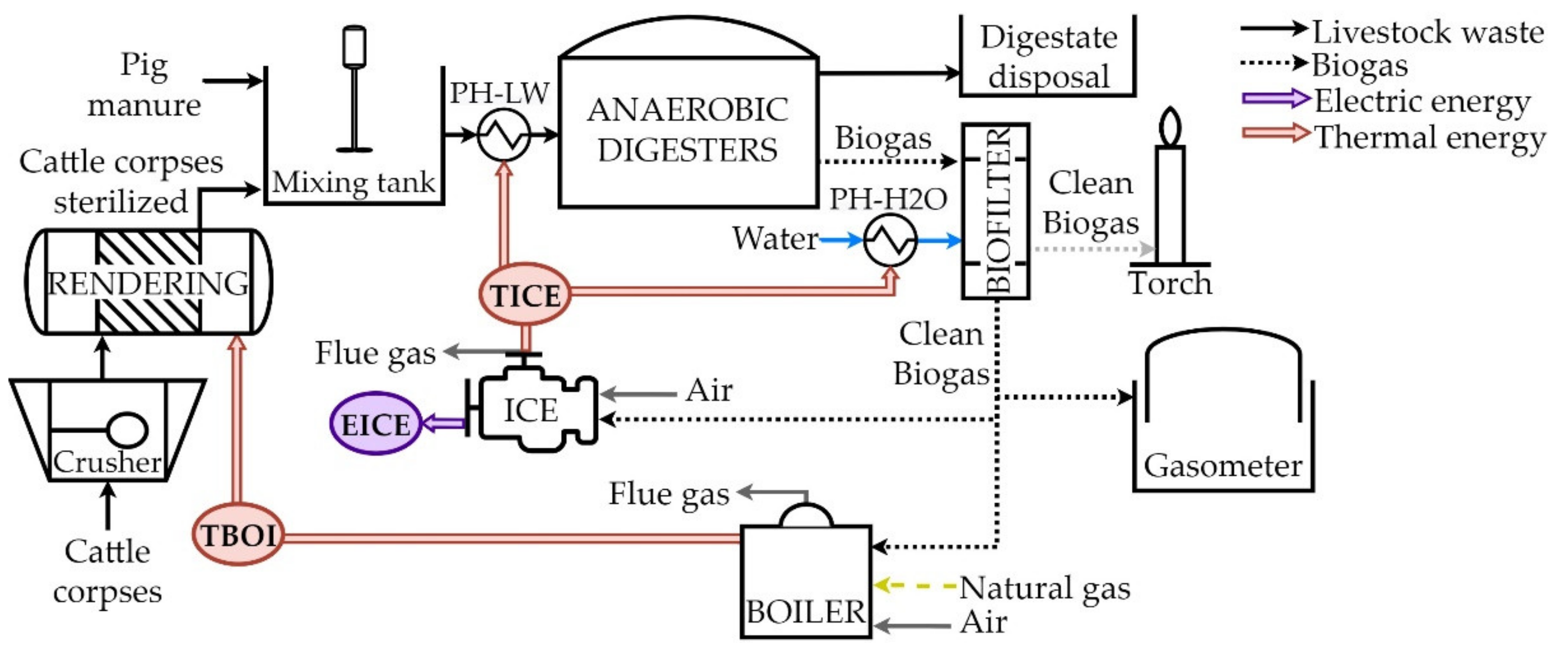
The livestock waste treatment plant studied is based on the anaerobic digestion (AD) of pig manure and cattle corpses, and a diagram of the process can be seen in Figure 1. This AD process produces biogas and an organic residual waste, which can be eventually used as fertilizer. A crusher, a rendering reactor and a mixing tank are the first processing steps in the plant aimed to condition the raw organic matter introduced in the system. The AD process takes place in two anaerobic digesters and, downstream, there exists a system to dispose digestate, a biofilter and a gasometer to condition and control the amount of produced biogas. The electric and thermal supply of the plant is covered by an internal combustion engine and a boiler.

After an initial crushing process, the cattle corpses stream is sterilized and prepared for digestion. Regulation (EU) no. 1069/2009 establishes the rendering process with saturated steam at 800 kPa as a suitable methodology for sterilization. The pre-treated organic matter is mixed with pig manure and, then the resulting livestock waste (LW) stream–composed by 90% pig manure and 10% cattle corpses is introduced in the anaerobic digestor. The AD process takes places at 170 kPa and 45–50 °C. The heat required to maintain the operating temperature is supplied by an internal combustion engine (ICE) through the sensible heat of its flue gas and refrigeration water. The preheater named PH-LW recovers this energy and supplies it to the LW mixture. This cogeneration ICE produces both thermal (TICE) and electrical load (EICE) which are integrated in the system or sold to the grid.

The biogas produced in the AD process has an outlet composition of 35% CO₂, 65% CH₄ and some ppm of H₂S. The solid-liquid stream eliminated from the digestor is directed to a post-digestor where biogas production is increased. The solid-liquid phase removed from this post-digestor contains stabilized and sterilized organic matter which can be safely used by surrounding farmers as fertilizer for their crops.

A biofilter is used to remove the content of H₂S in the biogas by adding air, water and nutrients. The outlet gas of this equipment has a composition of 35% CO₂ and 65% CH₄, with near zero ppm of H₂S (97% of removal efficiency in the biofilter). The power demanded to heat up the water consumed in the biofilter is supplied by the cogeneration ICE (TICE) through a preheater named PH-H2O.

A fraction of the clean biogas is stored in the gasometer while another fraction is fed into a boiler (80% boiler efficiency). The thermal load of this equipment (TBOI) produces steam for the rendering process. After its utilization, the condensed water is recirculated into the boiler to reduce the fuel combustion during operation. The remaining clean biogas is supplied to the cogeneration ICE to produce near 250 kWe (EICE) which is sold to the grid after covering the demand of the plant. Natural gas is fed into the ICE when the produced flowrate of biogas does not cover the requirement of the engine and no biogas is available in the gasometer. The electric efficiency of the ICE nearly achieves a 30% and the thermal efficiency circa 50%. The sources of the TICE are (i) the sensible heat of the flue gas and (ii) the refrigeration of the engine. Sensible heat of the flue gas at 450 °C is exchanged to the water (from 65 °C to 85 °C) used to cover the thermal demand at the inlet of the anaerobic digestor. The flue gas is sent to the stack at 115 °C. The main operation parameters of the LWTP equipment and streams are presented in

Table 1. Main operating parameters of livestock waste treatment plant equipment and streams.

LWTP Equipment Description		Stream	Inlet Stream	Outlet Stream	T	P	Electric Power	Thermal Power
			(kg/s)	(kg/s)	(°C)	(kPa)	(kWe)	(kWth)
Crusher	Cattle corpse crushing	Cattle corpses	0.15	0.15	Tamb	100	5.1
Rendering process	Cattle corpse sterilization	Saturated steam	0.085		170.4	800		166
		Saturated liquid		0.085	170.4	800
Mixing tank	Sterilized cattle corpse and pig manure mixing	Cattle corpses	0.15	0.15	Tamb	100	4.1
		Pig manure	1.16	1.16
PH-LW	Livestock waste preheating	TICE	5.13		85	180	0.8	429.3
				5.13	65	200
Anaerobic digesters	Livestock waste anaerobic digestion	Cattle corpses	0.15		45–50	170	11.1
		Pig manure	1.16
		Biogas		0.056	15–25	0.3
		Digestate		1.25		70
Biofilter	Biogas desulfurization	Biogas	0.056	0.054	25	100	3.5
		Water	0.04	0.04	35
PH-H2O	Biofilter water preheating	TICE	0.02		85	180	0.1	1.7
				0.02	65	200
Gasometer	Clean biogas storage	Biogas	0.011		25	100	0.3
Boiler	Steam production for rendering process	Biogas	0.011		Tamb	100		−227
		Air	0.138
		Saturated steam		0.085	170.4	800
		Condensed liquid	0.085		80	100
		Flue gas		0.149	656	100
ICE	Electric and thermal power production	Biogas	0.032		Tamb	100	−250	−431
		Air	0.417
		Flue gas		0.449	115	100
		TICE		5.15	85	180
			5.15		65	200

The negative sign of power indicates an energy release, while a positive value means a specific equipment requires an energy input.

. Currently, electric demand of the plant is around a 10% of the total produced electricity. While thermal demand includes the rendering process, the pre-heating requirement at the digestor inlet and the heat requirement of the biofilter.

This study proposes a new configuration which substitutes the current cogeneration ICE and boiler by a post-combustion Ca-looping CO₂ capture process together with a steam power cycle to cover thermal and electric demands of the plant. The main objective is to reduce CO₂ emissions in the global system in order to establish an innovative and technically feasible BECCS system.

2.2. Ca-Looping Carbon Capture Cycle

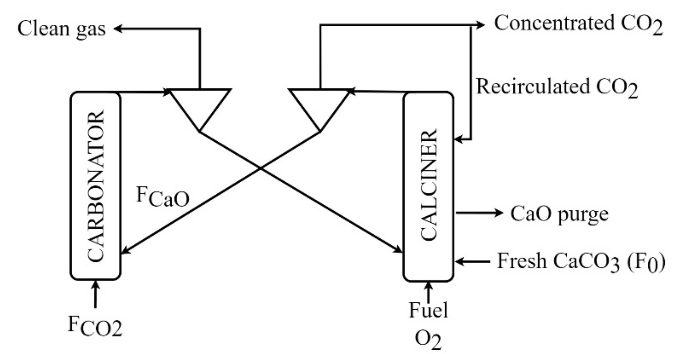
Ca-looping is one post-combustion carbon capture technology based on the carbonation/calcination reversible reaction shown in Equation (1). CO₂ from a flue gas stream is chemically absorbed in the carbonator and subsequently the absorbent material is regenerate in the calciner, as shown in Figure 2 [24]:

$${\mathrm{CaO}}_{\left(\mathrm{s}\right)}{+\mathrm{CO}}_{2 \left(\mathit{g}\right)}\leftrightarrows {\mathrm{CaCO}}_{3 \left(\mathrm{s}\right)} \Delta H_R^{°}=-178 \mathit{kJ}/\mathit{mol}$$

(1)

The exothermic carbonation reaction takes place at a temperature between 600 and 700 °C, where CO₂ reacts with calcium oxide to obtain calcium carbonate. Only a fraction of the calcium oxide introduced into the carbonator reacts and the active fraction will depend on the sorption activity of the particle population. Therefore, a mixture of calcium carbonate and unreacted calcium oxide is found at the carbonator outlet.

The clean gas stream with low CO₂ concentration (remaining non-captured CO₂) is separated from the solids leaving the carbonator and is emitted into the atmosphere. CaCO₃ calcination to regenerate the sorbent occurs instantaneously under the calciner operating conditions (910–930 °C) [25]. Thus, the solid output stream from calciner is 100% calcium oxide. The limestone introduced into the calciner comes from both the carbonation reaction and the input of fresh limestone. Oxyfuel combustion in the calciner covers the thermal demand of the endothermal calcination process. A CO₂ concentrated stream is the gas outlet of the calciner. The comburent required in the calciner is generated through an air separation unit and a portion of the concentrated CO₂ stream is recirculated to control temperature and fluidization conditions. The remaining CO₂ is refrigerated and compressed before being stored or sent to a utilization process.

The CaL process is less expensive than other carbon capture technologies given the use of limestone—a common in nature, non-toxic and cheap material—as a capture sorbent [26]. Temperatures above 600 °C in the CaL process allow the use of waste heat from capture process in power cycles or industrial processes. Heat integration potentially reduces the energy penalty associated with the capture process. The main drawback of this capture technology is the strong decay of the sorption activity of the CaO particles with the increasing number of cycles [27,28,29,30]. This phenomenon must be accounted when the capture process is modelled, as presented in Section 3.1.

2.3. Rankine Power Plant

The residual heat from the CaL capture system can be used to generate steam for the inlet of a Rankine cycle turbine. The residual heat from the carbon capture plant is used in a three-stage economizer, an evaporator and a final superheater. The implementation of a steam power cycle allows for bleeding a stream from the turbine to supply the steam requirements for the cattle corpse sterilization. The saturated liquid recovered from the rendering process is recycled to the low-pressure section of the power plant to increase the temperature of the stream from the condenser. Furthermore, the power plant (PP) also includes a degassifier which heats up the medium-pressure condensed liquid with part of the steam bleed from the turbine.

The Rankine cycle is designed and dimensioned in this study after calculating the available heat from the capture process. The proposed Rankine power plant replaces the current cogeneration ICE and the boiler which currently supplies the steam to the rendering process.

2.4. Proposed Integrated System LWTP-CaL-PP

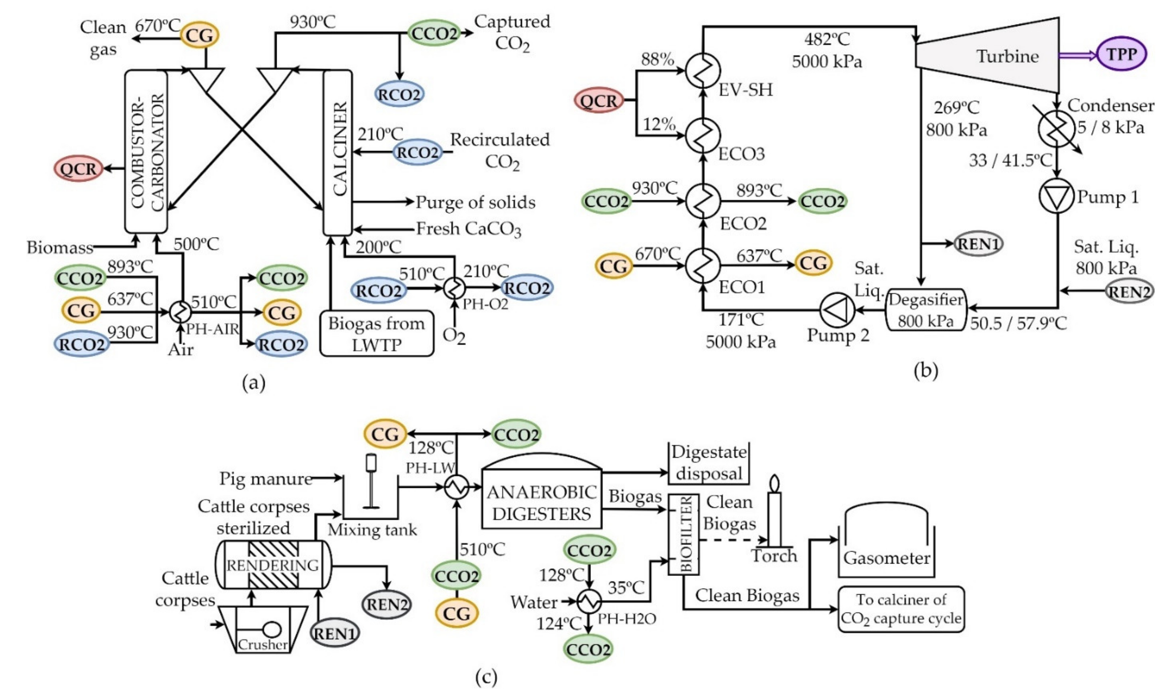
The proposed integration includes in the system the LWTP, a CaL carbon capture process and a PP as illustrated in Figure 3. The ICE and the boiler of the original LWTP (Figure 1) would be replaced by the Rankine power plant and the Ca-looping capture process to cover energy demand of the LWTP and produce electricity (Figure 3).

The thermal waste heat from the CaL carbon capture process (TCaL) could be used to cover the thermal energy demand of: (i) PP and (ii) LWTP. The CaL residual thermal energy (TCaL) comes from both the sensible heat of concentrated CO₂ and clean gases streams and thermal energy of biomass combustion and carbonation exothermic reactions taking place in the carbonator. The Rankine power plant will produce the electrical energy (EPP) and the required steam for the rendering process (TPP). The condensed steam from rendering process is recirculated after used to the low-pressure section of the Rankine cycle. The rest of the TCaL could be used to cover thermal energy demand of both the livestock waste preheater (PH-LW) and the biofilter water preheater (PH-H2O).

Furthermore, if the energy required by LWTP is fully covered the potential surplus of useful heat could be reintegrated into the CaL carbon capture process to preheat the air for biomass combustion in the carbonator or preheat the O₂ for biogas oxy-combustion.

Therefore, the waste energy from the CaL carbon capture system (TCaL) could be used considering their energy content and temperature level to reduce energy penalties in the follow way: (i) first to cover PP thermal energy demand, (ii) second to preheat the required comburents for biomass and biogas combustion in the CaL process, and (iii) third to supply the LWTP thermal energy demand.

3. Materials and Methods

The LWTP is modelled to define the energy requirements and establish the main operational parameters. The model of the capture process accounts for the reactors configuration, mass flows and sorbent properties to size the capture plant. The third modelling block is the steam power cycle which makes use from the available heat streams through a heat recovery boiler. The heat exchange network which accounts for the available heats and the thermal demand of (i) LWTP, (ii) carbon capture plant and (iii) power plant is the core of the modelling work. The integrated system is simulated to assess the behaviour of the three plants and study the influence of operation factors.

3.1. Ca-Looping Carbon Capture Model

The main limitation of this capture process is the significant decay of the carbonation activity of the sorbent particles with the increasing number of carbonation-calcination cycles [27,28,29,31,32]. The improvement of the global efficiency of the process is searched through the optimization of operation parameters such as fresh limestone flow, exhausted material flow or solid inventory in the reactor.

The conditions which favor the capture efficiency are large solid inventories in the system, large fresh limestones flows and large CaO/CO₂ ratios in the carbonator. These conditions compensate the degradation of the sorbent and provide adequate efficiencies of the capture system. The temperature spring from carbonator at 650 °C and calciner at 930 °C, thus, an important consumption of energy is expected given the large amounts of solid particles circulating from one reactor to the other one.

The initial sorption capacity of the Piaseck limestone is around 0.63 and the residual activity after a large number of calcination cycles is around 0.075 [32]. The equation which describes the activity of a Piaseck limestone particle after a number of calcination cycles is given by Equation (2) [33]:

$${\mathit{X}}_{\mathit{N}}=\frac{1}{\frac{1}{{1-\mathit{X}}_{\mathit{r}}}+\mathit{k}·\mathit{N}}{ + \mathit{X}}_{\mathit{r}}$$

(2)

where k is the decay constant (0.52), X_r is the residual activity (0.075) and N is the number of cycles suffered. There is a distribution of particle ages in the system and to calculate the average conversion of the total population of solid particles (X_ave), the distribution of population ages must be accounted through Equation (3). The percentage of solid particles with the same number of calcination cycles is represented by the variable r_N and given in Equation (4):

$${\mathit{X}}_{\mathit{ave}} ={\displaystyle \sum }_{\mathit{N}=1}^{\mathit{N}=∾}{\mathit{r}}_{\mathit{N}}{·\mathit{X}}_{\mathit{N}}$$

(3)

$${\mathit{r}}_{\mathit{N}} = \frac{\frac{{\mathit{F}}_0}{{\mathit{F}}_{\mathit{CaO}}}}{{\left(1+\frac{{\mathit{F}}_0}{{\mathit{F}}_{\mathit{CaO}}}\right)}^{\mathit{N}}}$$

(4)

where F_CaO is the molar flow of CaO entering the carbonator and Fo represents the flow of fresh limestone.

The average sorption activity under the presence of sulphur compounds in the flue gas must be corrected since part of the sorbent will react with the sulphur dioxide Equation (5). Finally, the capture efficiency of the system is determined through Equation (6):

$${\mathit{X}}_{\mathrm{ave}} ={\displaystyle \sum }_{\mathit{N}=1}^{\mathit{N}=∾}{\mathit{r}}_{\mathit{N}}{·\mathit{X}}_{\mathit{N}}-\frac{{\mathit{F}}_{\mathrm{CO}2}}{{\mathit{F}}_0{*\mathit{r}}_{\mathit{C}/\mathrm{s}}}$$

(5)

$${\mathit{\eta }}_{\mathit{capt}}= \mathit{R}·{\mathit{X}}_{\mathit{ave}} = \frac{{\mathit{F}}_{\mathit{CaO}}}{{\mathit{F}}_{\mathit{CO}2}}·{\mathit{X}}_{\mathit{ave}}$$

(6)

where F_CO2 is the molar flow of CO₂ entering the carbonator.

3.2. Methodology for Sizing Carbon Capture, Power Plant and Heat Exchange Network

The criteria for sizing the equipment includes, in the first place, the coverage of the thermal requirements of the LWTP, and, then, the coverage of electric demand of the LWTP. The flow of biogas, currently consumed in the ICE and the boiler, will be used in the calciner to provide heat for the instantaneous sorbent regeneration through oxyfuel combustion. Once the calciner is sized, the carbonator is dimensioned using the model previously described.

The available heat flows from the carbon capture cycle are (i) the sensible heat of the clean flue gas stream at the outlet of the combustor-carbonator (CG), (ii) the sensible heat of the concentrated CO₂ stream (CCO2), (iii) the sensible heat of the recirculated CO₂ stream (RCO2) and (iv) the heat from biomass combustion and the carbonation reaction heat (QCR). These available heat flows from the carbon capture cycle are used to cover the thermal demand of the LWTP and the Rankine power cycle.

The Rankine power cycle makes use of the energy released in the combustion of biomass and the capture process to generate steam in the condition to be introduce into the turbine inlet. The composition of the biomass fed into the carbonator is provided in

Table 2. Ultimate analysis, LHV, ash and moisture content of the biomass used in the boiler.

Biomass Composition	Ultimate Analysis (wt%)
Carbon	44.28
Hydrogen	0.05
Nitrogen	0.69
Sulfur	4.96
Oxygen	32.46
Ash	7.56
Moisture	10.00
LHV (MJ/kg)	14.97

together with its low heating value. It also provides the content of moisture and ashes of the solid biomass. Part of these ashes are accumulated in the fluidized beds and part are purged from the system mixed with the solid sorbent purge stream in the calciner (exhausted CaO and ashes).

The high temperatures involved in the capture system make possible the recovery of most of the energy content of the fuel and produce energy in a power cycle [34,35,36]. The heat exchangers which allow to achieve the steam conditions required in the turbine inlet make use of the economizer and a boiler with superheating step. The cycle also includes a degasifier at 800 kPa and a condenser operating at 5 kPa. This condensing pressure can be assured given the annual range of temperatures in the selected location [37]. The temperatures ranges from −5 °C to 32 °C, which correspond to saturation pressures below 5 kPa. Nevertheless, a condenser pressure above 5 kPa has been assumed during the operating period with the highest ambient temperature. Thus, 8 kPa as condensing pressure for two months of equivalent operation (1300 h per year approximately) ensures the required temperature gradient between the condensing steam and the cooling medium.

The objective in the design of the heat exchange network is to make the best use of the sensible heat of the gas streams of the carbon capture cycle, accounting for their energy content and level of temperature. First, the thermal demand of the LWTP must be covered. Once this heat requirement is fulfilled, the excess of available heat will cover the thermal demands of the capture process itself to reduce the energy penalty of the capture such as comburent preheating in both reactors.

4. Technical Results and Assessment

In this section, the results obtained from the simulations sequentially. First, results from the carbon capture process model. Then, the dimensions obtained for the capture and power cycles. Finally, the analysis of the heat exchange network and the carbon balance.

4.1. Carbon Capture Process

The target capture efficiency is set in 90% of the CO₂ contained in the flue gas from the combustion of biomass [25]. First, a sensitivity analysis of the solid mass flow purged in the calciner and the molar ratio CaO/CO₂ at the carbonator was performed.

A high value of R implies very large solid circulation, increasing the amount of energy required to increase the temperature of solid population up to 900 °C in the calciner. As shown in Figure 4, the demand for calcination heat in the calciner is larger with higher solid circulation between reactors in the Ca-looping since it leads to higher carbonation efficiencies and the amount of limestone generated in the carbonation reaction is increased. The technical feasibility of the system may be compromised when selecting values of R over 5 given the great increase of solid circulation between reactors. Solid handling becomes more complex, the investment cost much larger and the energy consumptions skyrocket. The chosen parameters for the sizing of the carbon capture process are a R of 4.5 and a solid purge percentage of 3%, which lead to a X_ave of 20% and a carbon capture efficiency around 90%.

∙ The energy released from the carbon capture system calculated from the model presented in Section 3.1 includes four main terms defined as follows:

• Heat released in the carbonator (QCR). This thermal energy is released in the carbonator reactor through the exothermal carbonation reaction and the combustion of biomass. The amount of heat which can be produced in this equipment is 2156 kW,
• The sensitive heat of the clean gas stream at the outlet of the carbonator (CG). The sensitive heat of this stream for the size and operation conditions of the capture cycle achieves 454 kW,
• The sensitive heat of the captured CO₂ at the outlet of the calciner (CCO2). The stream of captured CO₂ carries a sensitive heat of 415 kW and
• The sensitive heat of the captured CO₂ which is recirculated to the calciner (RCO2). The heat transported by this carbon dioxide stream is 86 kW.

The carbon capture cycle presents thermal demands which correspond to the preheating of comburents for both reactors. In the carbonator, the air requires a preheating temperature of near 500 °C (324.6 kW) and, in the calciner, the oxygen requires an inlet temperature of 200 °C (21.8 kW).

4.2. Rankine Power Cycle

The power cycle makes use of part of the heat content of the clean flue gas and the sensitive heat of the captured CO₂ at the outlet of the calciner to increase the inlet temperature of the water to economizer 1 and economizer 2, respectively. The 88% of the heat released in the carbonator (combustion and carbonation reaction) is directed to the heat recovery steam generator of the power cycle (evaporator + superheater). The rest of the heat is sent to the third stage of the economizer, 12%.

The size of the steam turbine is 750 kWe with a thermodynamic efficiency of 80%. The flowrate at the turbine inlet is 0.825 kg/s and the properties of the live steam at the entrance of the turbine are 482 °C and 5000 kPa. The quality of the wet steam leaving the turbine is 92% when the condenser pressure is 5 kPa, while the quality rises up to 93% during the operating period in which the condenser pressure is 8 kPa. The properties of the live steam were set through a sensitivity analysis carried out to maximize the electricity produced and considering typical inlet live steam input parameters for power turbines below 1 MW [38]. The production of electricity considering the required steam bleed in the turbine amounts up to 698.90 kWe for 5 kPa condensing pressure and 677.30 kWe during the highest ambient temperature period when condenser pressure is 8 kPa. Part of this electricity is used to cover the electrical demands of the LWTP and the carbon capture cycle and, once the demands are covered, the remaining electricity is sold to the grid, 694.10 kWe when the condenser of the power cycle works at 5 kPa and 672.50 kWe for the operating period with 8 kPa as condensing pressure.

A fraction of the bleed from the turbine at 800 kPa is used to cover the steam demand of the rendering stage in the LWTP. The condensate from this process is recycled to the Rankine cycle increasing the temperature of the liquid at the outlet of the condenser up to 50.5 °C or 57.9 °C if the condenser pressure is 5 kPa or 8 kPa, respectively. Meanwhile, the remaining part of the turbine steam bleed is directed to the degasifier. The pressure of the desgasifer is established at 800 kPa after another sensitivity analysis to maximize the power output also taking into account the requirement of process steam properties in the LWTP and the strong limitations for small size steam turbine to implement more than one bleed.

The electrical efficiency of the original LWTP amounts 16%, Equation (7), and is calculated comparing the available energy to be used and the energy content of the fuel used in the plant, Q_biogas,LWTP. The available energy is the difference between the electrical energy generated by the ICE, W_net,LWTP, and the electrical energy consumed in the LWTP, W_aux,LWTP:

$${\mathit{\eta }}_{\mathit{ref}}=\frac{{\mathit{W}}_{\mathit{net}, \mathit{LWTP}} {- \mathit{W}}_{\mathit{aux},\mathit{LWTP}}}{{\mathit{Q}}_{\mathit{biogas},\mathit{LWTP}}}$$

(7)

The efficiency of the integrated plant achieves a 19% and is determined through Equation (8) where the available energy is calculated as the difference between the electrical energy generated by the Rankine cycle, W_net,PP, and the electrical energy consumed in the plant. The energy consumed in the integrated system accounts for the auxiliary consumption in the LWTP, the auxiliary consumption in the carbon capture and power plant (5% of the net produced electricity) and the consumption of the air separation unit, W_aux,LWTP + W_aux,PP + W_ASU. The energy consumed in the integrated plant accounts for the energy content of the biomass and biogas fuels, Q_CMB,biogas + Q_CMB,biomass.

$${\mathit{\eta }}_{\mathit{CaL}-\mathit{LWTP}}=\frac{{\mathit{W}}_{\mathrm{net},\mathrm{PP}} {- \mathit{W}}_{\mathit{aux}, \mathit{LWTP}}{ - \mathit{W}}_{\mathit{aux},\mathit{PP} }{- \mathit{W}}_{\mathit{ASU}}}{{\mathit{Q}}_{\mathit{CMB} \mathit{biomass} }{+ \mathit{Q}}_{\mathit{CMB} \mathit{biogas}}}$$

(8)

The energy efficiency of the LWTP integrated to the carbon capture and Rankine cycles results to be three percentage points higher than the original facility. Therefore, the proposed integration results energetically feasible.

4.3. Heat Exchange Network Analysis

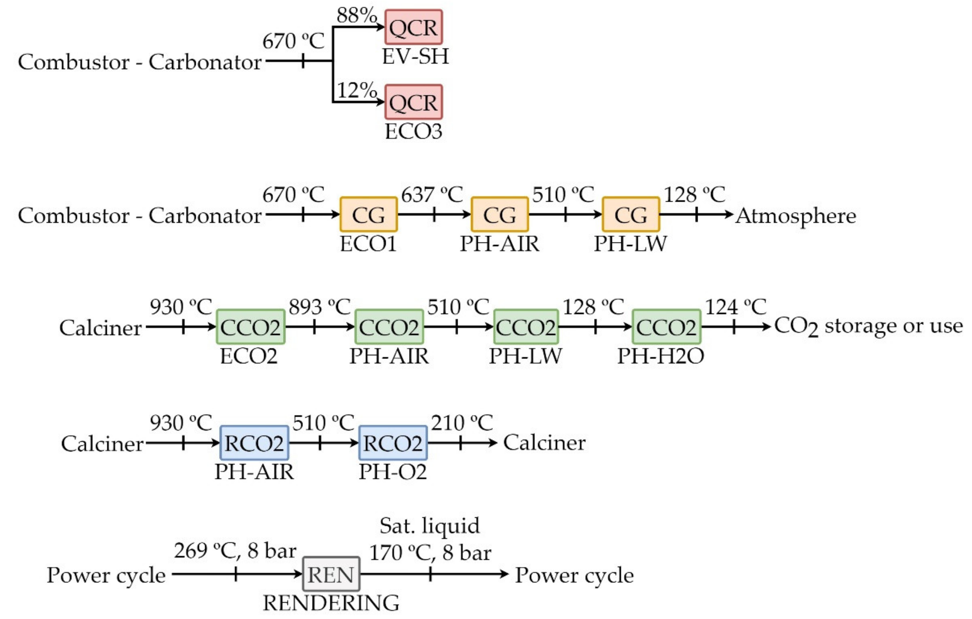
The sources of available heat are gathered in

Table 3. Description of the available heat streams in the heat exchange network.

Heat Source	Heat Requirement		Tin (°C)	Tfin (°C)	Heat Flow (kW)
QCR	Surplus heat CR	Evaporator + Superheater (88%) (EV+SH)	670	670	1890
		Third stage economizer (12%) (ECO3)	670	670	266
CG	Gas flow leaving CR	First stage economizer (ECO1)	670	637	24
		Preheating air inlet to CR	637	510	95
		Heating livestock waste input to digester	510	128	266
CCO2	CO2 captured	Second stage economizer (ECO2)	930	893	20
		Preheating air inlet to CR	893	510	187
		Heating livestock waste input to digester	510	128	169
		Heating water input to biofilter	128	124	2
RCO2	CO2 recirculated to CL	Preheating air inlet to CR	930	510	44
		Preheating O2 inlet to CL	510	210	27
REN	Steam rendering	Rendering process heat required (REN1)	269	170.4	192.6
		Rendering to Steam cycle (REN2)	170.4	170.4	59

and Figure 5 correspond to: (i) QCR, heat from the carbonator reactor, (ii) CG, sensible heat of clean gas flow rate from carbonator reactor, (iii) CCO2, sensible heat of CO₂ captured flow rate from calciner reactor, (iv) RCO2, sensible heat of CO₂ flow stream recirculated to calciner reactor, (v) REN, steam flow rate from power cycle. The elements which demand heat are: (i) superheater (SH) + evaporator (EV), (ii) first stage economizer (ECO1), second stage economizer (ECO2) and third stage economizer (ECO3), (iii) carbonator air preheater (PH-AIR), (iv) calciner O₂ preheater (PH-O2), (v) livestock waste preheater (PH-LW), (vi) biofilter water preheater (PH-H2O) and (vii) the rendering process (REN). The diagram of the heat exchange network is illustrated in Figure 6.

The clean gas stream from carbonator provides heat to different stages: economizer 1, air preheating (biomass combustion) and preheating of livestock wastes. The energy content of the stream of captured CO₂ (CCO2) is used to cover the demand of the following processes: (i) the second economizer, (ii) preheating of air (comburent for biomass combustion), (iii) the preheating of livestock wastes at the inlet of the digestor and (iv) thermal energy to the biofilter located at the outlet of the LWTP digestors. The sensitive heat of the CO₂-rich gas stream which is recirculated to the calciner (RCO2) is required to cover (i) part of the thermal demand of the air preheating and (ii) the thermal demand required to preheat the oxygen (biogas comburent). Lastly, the energy released in the carbonator (QCR) from the biomass combustion and the carbonation reaction are used to cover the thermal demand in (i) the third economizer and (ii) the evaporator-superheater stage. These two stages correspond to the last three stages of the heat recovery steam generation (HRSG) in the Rankine cycle.

Furthermore, part of the steam bleed at 800 kPa (REN1) from the steam turbine is used in the rendering process of the LWTP. The condensate of this stream (REN2) is recirculated again to the low-pressure equipment of the cycle.

The high temperature of the gases after the first and second economizers makes these streams still useful. The energy content of these gases with a sensitive heat of 824 kW (CG + CCO2), together with the energy from the recirculated stream of CO₂ (RCO2), sensitive heat at the outlet of the calciner 86 kW, are employed to the preheating of air fed into the carbonator-boiler up to 500 °C. The temperature of the gases after this exchange of heat with the air is reduced to 510 °C. The sensitive heat of the gas streams leaving the heat exchanger (except the recirculated stream of CO₂) is used to cover the thermal demand of the livestock wastes at the inlet of the digester, 431 kW. The temperature of the gas stream is reduced down to 128 °C during this heat exchange. The clean gas stream is, then, emitted to the atmosphere. The energy content of the captured CO₂ stream after this second exchange is used to supply thermal energy to the biofilter in the LWTP. Its temperature is reduced down to 124 °C. The thermal demand for the preheating of oxygen used as comburent in oxyfuel combustion of biogas in the calciner is covered with the sensitive heat of the recirculated CO₂ stream after the first heat exchange. The final temperature of this stream is 210 °C which corresponds to the temperature of the recirculated stream of CO₂.

4.4. Carbon Balance

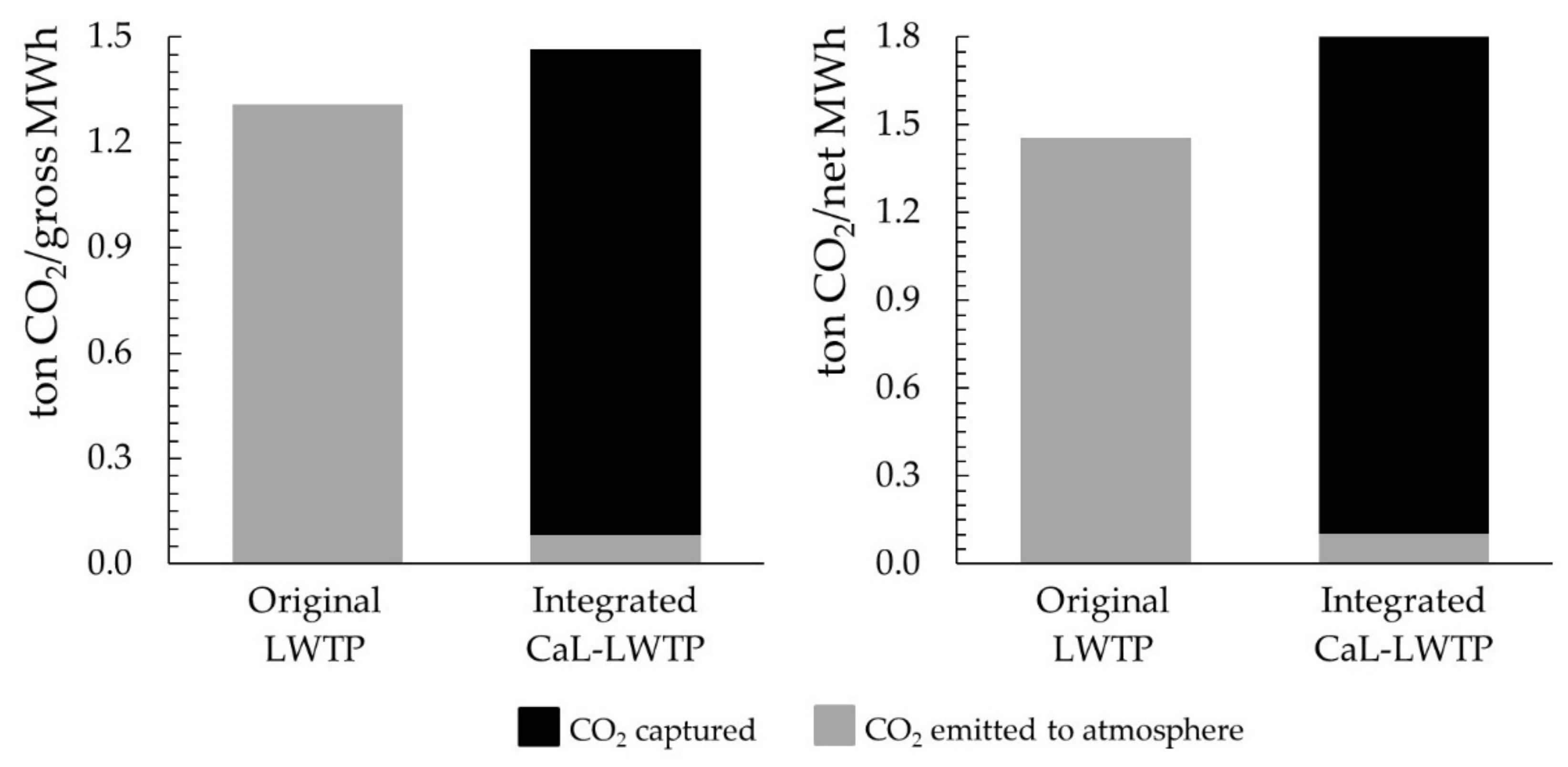
A carbon balance of the original plant and the proposed integrated facility quantitatively compares their specific emissions. The original plant releases CO₂ emissions from the biogas combustion in both the boiler and the ICE. After integration with the carbon capture cycle, carbon emissions are limited to the CO₂ content in the clean gas stream at the outlet of the calciner, nearly a 10% of the CO₂ generated in the biomass combustion, and the CO₂ released in the calcination of the fresh limestone added to the cyclic process.

Table 4. Electric power produced in LWTP respect to integration.

Electrical Energy Flow Description		LWTP	CaL-LWTP
Electric production (MWh/year)	Power cycle		4136.5
	ICE	1500
Electric consumption (MWh/year)	Auxiliaries LWTP (pumps, agitators, compressors, blowers, crusher)	150	150
	Auxiliaries CaL & PP (5% of power cycle electric production)		206.8
	ASU (CaL CO2 capture cycle)		456
Electric power sold (MWh/year)		1350	3323.7

presents the values of annual consumption and generation of electricity (MWh/year) for both the original situation of the LWTP and the proposed integration with CaL carbon capture. Considering a variable condensing pressure throughout the year, the net electricity generated during a fifth of the operating period is 3% lower than the net power generated the rest of the period. The amount of electricity produced by the power cycle in the integrated system is almost 2.75 times larger than the production of the ICE in the original LWTP. Considering the consumption of auxiliary equipment, an 80% of the produced electricity is sold to the grid in the integrated system while a 90% of the electricity produced by the ICE in the original plant is sold to the grid. This is mainly due to the electrical consumption of the air separation unit.

Considering 6000 h of operation per year, the specific carbon emissions per produced MWh of the original LWTP is 16 times larger than the specific carbon emission of the proposed CaL-LWTP when the electrical consumptions are not accounted, Figure 7. Besides, over a 90% of specific carbon emissions of the original LWTP could be avoided. When electricity demand of both facilities is considered, the specific carbon emissions of the original LWTP are 14 times larger than the proposed integrated system, Figure 7.

To assess the economic feasibility of this integrated facility and ensure the deployment of these systems, the evolution of the cost of allowances of CO₂ emissions are a key factor to consider. During 2018 a process of rising prices took place from 8.34 to €22.57 at the end of the year [39]. The price is €30.54 on December 2020 and the trend observed leads to a prediction of approximately €35 per avoided equivalent CO₂ ton by the end of 2021.

The avoided emissions calculated in this study as the difference between the emissions of the original LWTP and the emissions of the integrated CaL-LWTP, leads to savings of 1620 tons of CO₂ per year, thus, an 82% of the original emissions are avoided. Taking 24.66 € as a conservative value of the average CO₂ ton cost in 2020, the LWTP could avoid the expense of 39,949.2 €/year only associated to the non-emitted tons of CO₂ through the implementation of the carbon capture system.

5. Economic Assessment

Once the technical assessment of the integrated plant is presented, the required elements for a proper economic analysis of the proposed configuration are presented. These concepts include the initial investment, the estimation of operation costs, the maintenance costs and the net cash flow associated to the construction and operation of the proposed facility.

The present analysis is carried out using PRESTO software [40] and thermo-economic models for: (i) steam Rankine cycles [41], (ii) Ca-looping post-combustion CO₂ capture systems [42] and (iii) biomass-fired power plants [43] to estimate the capital investment cost of the proposed facility. Data compiled on the specific investment costs and operation & maintenance costs of biomass steam power plants are also input to our calculations [44].

5.1. Initial Investment and Commisioning of the Plant

The required investments to build the carbon capture system together with the Rankine power cycle described in the previous sections are shown in

Table 5. Investment cost and commissioning of the integrated facilities (carbon capture and power plants).

Investment Cost and Commissioning Description	Cost
	(€)
Cleaning and clearing land	351.80
Ground movement	571.16
Foundations	12,041.90
Metallic structure	246,841.05
Security and health	99,710.00
Cyclones and loop-seal valves	8743.80
Commercial equipment	1,612,607.27
Combustor—Carbonator	115,042.76
Calciner	47,288.92
Power cycle	1,028,072.68
Assembly of structures and pipes	127,833.33
Commissioning facility	102,266.67
Total cost	3,401,371.34

. The investment cost required to implement the facility includes the preparation of the soil, the cleaning and soil movement to build the cementation and metallic structure required to support the reactors of the carbon capture and the Rankine cycle. Additionally, the investment cost of the main and auxiliary equipment required in the carbon cycle and the Rankine cycle are presented considering both building and commissioning as well as the investment in health and security issues. The total investment cost amounts up to €3,401,371.34. This value does not include the VAT since it is not accounted as part of the initial investment under current tax regulations.

The costs associated to licenses, commissioning and operation contracts are embedded into the global costs of the activity of the project. Thus, they are not considered in this section since a pre-existing activity (LWTP operation) is required for the proposed project.

5.2. Operation Costs

The operation costs of the carbon capture process and the Rankine steam cycle are described in this section. 6000 operating h per year are considered in the assessment to account for the maintenance shut-downs or potential emergency stops. This section includes those variable costs related to:

• Electric consumption of equipment related to the carbon capture cycle and Rankine power cycle.
• Water consumption in the Rankine power cycle.
• Biomass consumption in the boiler-carbonator reactor in the carbon capture cycle.
• Limestone consumption in the calciner of the carbon capture cycle.

With regard to the electric consumption and considering the trends of electricity cost [45], an average annual cost of the electricity is set in 0.11 €/kWh. In this case study, the required electricity in the facility is determined by the consumptions of auxiliary equipment, blowers, feeding screws, the air separation unit and the pumps of the Rankine power cycle. These consumptions and costs are detailed in

Table 6. Electric power demand annual cost in the capture plant and Rankine cycle [45].

Electric Power Demand Description	Power	Consumption	Annual Cost
	(kW)	(kWh/Year)	(€/Year)
Auxiliaries CaL CO2 capture cycle	34.47	206,800	22,748
ASU	76	456,000	50,160
Power cycle pumping train	4.80	28,800	3168
Total annual cost			76,076

. The annual cost of electric consumption in the facility, considering an average annual price corresponding to 2008–2020 period, rises up to 76,076 €/year.

The water consumption amounts up to 0.825 kg/s and it is used as steam in the Rankine power cycle and to cover the requirements of the rendering process of the LWTP. The calculation considers the price of the m³ of water in the province of Soria (Spain) [46] and they are shown in Equations (9) and (10). The annual cost of water consumption of the Rankine cycle is 9848.54 €/year, considering an average price of the m³ of industrial water within the province of Soria:

$$\frac{\mathrm{Water} \mathrm{consumption}}{\mathrm{year}}=\frac{0.825 \mathrm{kg}}{\mathrm{s}}·\frac{{1 \mathrm{m}}^3}{1000 \mathrm{kg}}·\frac{3600 \mathrm{s}}{1 \mathrm{h}}·\frac{6000 \mathrm{h}}{\mathrm{year}}=\frac{\mathrm{17,828.64}{ \mathrm{m}}^3 \mathrm{water} }{\mathrm{year}}$$

(9)

$$\frac{\mathrm{Water} \mathrm{consumption} \mathrm{cost}}{\mathrm{year}}=\frac{\mathrm{17,828.64}{ \mathrm{m}}^3 \mathrm{water}}{\mathrm{year}}·\frac{0.5524 €}{{\mathrm{m}}^3 \mathrm{water}}=\frac{\mathrm{9,848.54} €}{\mathrm{year}}$$

(10)

The consumption of biomass consumption in the boiler-carbonator raises up to 0.1025 kg/s. The calculations accounts for the average annual cost of biomass in the period 2014–2020 [47] which results in 109.91 €/ton of chips. The results are shown in Equations (11) and (12). The annual cost related to the consumption of biomass in the boiler-carbonator, accounts for an average annual price of the biomass chip of 243,340.74 €/year, corresponding to the period 2003–2017:

$$\frac{\mathrm{Biomass} \mathrm{consumption}}{\mathrm{year}}=\frac{0.1025 \mathrm{kg}}{\mathrm{s}}·\frac{1 \mathrm{ton}}{1000 \mathrm{kg}}·\frac{3600 \mathrm{s}}{1 \mathrm{h}}·\frac{6000 \mathrm{h}}{\mathrm{year}}=\frac{2214 \mathrm{ton} \mathrm{biomass}}{\mathrm{year}}$$

(11)

$$\frac{\mathrm{Biomass} \mathrm{consumption} \mathrm{cost}}{\mathrm{year}}=\frac{2214 \mathrm{ton} \mathrm{biomass}}{\mathrm{year}}·\frac{109.91 €}{\mathrm{ton} \mathrm{biomass}}=\frac{\mathrm{243,340.70} €}{\mathrm{year}}$$

(12)

The fresh limestone consumption required to keep a significant average conversion of the calcium oxide (around 20%) amounts up to 0.05263 kg/s. The average price of the fresh limestone is 6 €/ton [26], and the calculations are presented in Equations (13) and (14):

$$\frac{{\mathrm{Fresh} \mathrm{CaCO}}_3 \mathrm{consumption}}{\mathrm{year}}=\frac{0.05263 \mathrm{kg}}{\mathrm{s}}·\frac{1 \mathrm{ton}}{1000 \mathrm{kg}}·\frac{3600 \mathrm{s}}{1 \mathrm{h}}·\frac{6000 \mathrm{h}}{\mathrm{year}}=\frac{{1136.81 \mathrm{ton} \mathrm{CaCO}}_3}{\mathrm{year}}$$

(13)

$$\frac{{\mathrm{Fresh} \mathrm{CaCO}}_3 \mathrm{consumption} \mathrm{cost}}{\mathrm{year}}=\frac{{1136.81 \mathrm{ton} \mathrm{CaCO}}_3}{\mathit{a}\mathit{ñ}\mathit{o}}·\frac{6 €}{{\mathrm{ton} \mathrm{CaCO}}_3}=\frac{6820.85 €}{\mathrm{year}}$$

(14)

Lastly, the sorbent and ash purge amount up to 0.0373 kg/s. The unit cost of the CaO and ash disposal is 10 €/ton [48], and the calculations are presented in Equations (15) and (16):

$$\frac{\mathrm{CaO} \mathrm{and} \mathrm{ash} \mathrm{purge}}{\mathrm{year}}=\frac{0.0373 \mathrm{kg}}{\mathrm{s}}·\frac{1 \mathrm{ton}}{1000 \mathrm{kg}}·\frac{3600 \mathrm{s}}{1 \mathrm{h}}·\frac{6000 \mathrm{h}}{\mathrm{year}}=\frac{805.68 \mathrm{ton} \mathrm{CaO} + \mathrm{ash}}{\mathrm{year}}$$

(15)

$$\frac{\mathrm{CaO} \mathrm{and} \mathrm{ash} \mathrm{disposal} \mathrm{cost}}{\mathrm{year}}=\frac{{805.68 \mathrm{ton} \mathrm{CaCO}}_3}{\mathit{a}\mathit{ñ}\mathit{o}}·\frac{10 €}{{\mathrm{ton} \mathrm{CaCO}}_3}=\frac{\mathrm{8,056.80} €}{\mathrm{year}}$$

(16)

Therefore, the annual operation cost is composed by the consumption of raw materials (water, biomass and fresh limestone), sorbent and ash disposal and the electric demand of the carbon capture cycle and the Rankine power cycle. It amounts up to 344,142.93 €/year and is considered as a constant annual variable cost during the lifetime of the integrated facility since the influence of inflation is not considered in this study.

5.3. Manteinance Costs

The maintenance costs are considered in this study as fixed costs which must be paid out in the due time recommended by the manufacturers despite the operation factor of the equipment in order to enlarge their lifetime.

The maintenance cost of the most significant equipment are detailed in

Table 7. Annual maintenance cost of the equipment in the capture plant and Rankine cycle.

Equipment Maintenance Operation Description		Annual Cost (10% on Equipment Cost)
		(€/Year)
Combustor-carbonator blower	Engine and blades change	519.00
Bag filters	Replacement filter elements	5982.60
Calciner blower	Engine and blades change	432.50
ASU	Equipment elements change	10,000.00
Endless screw for biomass	Engine/reducer and screw change	396.28
Endless screw for fresh limestone	Engine/reducer and screw change	133.97
Valves	Impellers and engines change	1,100.00
Power cycle pumps and turbine	Engine and blades change	40,948.40
Heat exchangers	Cleaning, plates and gaskets change	9204.00
Total annual cost		68,716.75

. However, the legal maintenance costs are not accounted. An annual maintenance cost of 68,716.75 €/year was estimated. It is considered as a fixed cost of the facility to be considered along the total lifetime.

5.4. Net Cash Flow of the Project

The assumptions made to calculate the incomes of the project are presented in the following. The project assumes that the consumption of natural gas is negligible compared to the biogas utilization since natural gas would only be used in the case that the biogas storage tank is empty. This situation is not expected to occur under normal operation of the LWTP. The requirements of steam in the rendering process is covered with part of the energy from the produced biogas. Therefore, the economic savings related to the reduction of natural gas consumption in the proposed configuration is almost zero. For this reason, the saving related to natural gas consumption is not accounted as a reduction of fixed costs.

The proposed project is considered to be subjected to the Emission Trading System. Since carbon capture is the main objective of the project, the future work should be directed to technically and economically study the condition and storage of the captured CO₂ for its possible valorization. The sale of produced electricity, once the requirements of the LWTP, the CaL and the Rankine PP are covered, is considered as an income.

5.4.1. Emission Trading System

For the calculation of emissions reduction, the difference of CO₂ emissions to the atmosphere between the current facility and the integrated project. Under the current situation, the carbon emissions come from biogas combustion in the boiler and the ICE. After integration, the carbon emissions to the atmosphere are only those contained in the clean gas leaving the boiler-carbonator (non-captured carbon emissions in the carbonation reaction). The avoided carbon emissions rise up to 1620 CO₂ ton per year, independently of the origin of those emissions, as detailed in Section 4.4.

Therefore, the incomes obtained from the Emission Trading System considering an average price of the avoided and verified CO₂ ton of 24.66 €/ton CO₂ (average annual value of 2020). These incomes are calculated through Equation (17).

5.4.2. Savings from Carbon Captured

$$\frac{{\mathrm{Avoided} \mathrm{CO}}_2 \mathrm{incomes}}{\mathrm{year}}=\frac{{1620 \mathrm{ton} \mathrm{CO}}_2}{\mathrm{year}}·\frac{24.66 €}{{\mathrm{ton} \mathrm{CO}}_2}=\frac{\mathrm{39,949.2} €}{\mathrm{year}}$$

(17)

If the captured CO₂ is the final storage, a methodology which accounts for the validation of negative carbon emissions should be considered. The potential annual income related to these negative emissions could be calculated through Equation (18).

$$\frac{{\mathrm{Captured} \mathrm{CO}}_2 \mathrm{incomes}}{\mathrm{year}}=\frac{{5713.2 \mathrm{ton} \mathrm{CO}}_2}{\mathrm{year}}·\frac{9.7 €}{{\mathrm{ton} \mathrm{CO}}_2}=\frac{\mathrm{55,418.04} €}{\mathrm{year}}$$

(18)

5.4.3. Sale of Electricity

The Rankine cycle generates 689.42 kWe net electricity, considering 672.50 kWe of net production during a fifth of the operating period, while the rest of the period the net power amounts to 694.10 kWe. After covering the electric demand of the LWTP (25 kWe), the pumping train of the Rankine cycle (4.80 kWe), the ASU power consumption (76 kWe) and the auxiliary equipment in the carbon capture cyle (34.47 kWe), 553.95 kWe are sold to the electric grid. The electric production and the related incomes considering 6000 h of annual operation are calculated through Equations (19-20). The price of electricity has been assumed as 46.78 €/MWh, an average value of the last ten years, 2010–2019 [49]:

$$\frac{\mathrm{Electric} \mathrm{production}}{\mathrm{year}}=553.95 \mathrm{kW}·\frac{1 \mathrm{MW}}{1000 \mathrm{kW}}·\frac{6000 \mathrm{h}}{\mathrm{year}}=\frac{3323.70 \mathrm{MWh}}{\mathrm{year}}$$

(19)

$$\frac{\mathrm{Electric} \mathrm{sale} \mathrm{incomes}}{\mathrm{year}}=\frac{3323.70 \mathrm{MWh}}{\mathrm{year}}·\frac{46.78 €}{\mathrm{MWh}}=\frac{\mathrm{155,482.69} €}{\mathrm{year}}$$

(20)

Thus, the total annual incomes achieve the value 250,849.93 €/year considering average prices of electricity sale, carbon allowances and CO₂ as raw material.

5.5. Equilibrium Point

The data presented in the previous sections are used to calculate the cash flow of the project and determine the equilibrium point according the initial investment, the costs and the possible incomes. The Net Present Value (NPV) and Internal Rate of Return (IRR) of the project are calculated based on the provided information.

Two projections of cash flow were done since the current level of savings and incomes does not lead to economic feasibility regarding the payback time. Besides current conditions, the minimum price of the produced electricity to determine the minimum required income which lead to an economically feasible project considering the payback time of the investment. The electricity cost has been calculated as Levelized Cost Of Electricity, LCOE. The minimum incomes are related to the saved carbon emissions and the potential of CO₂ as a chemical. The two scenarios considered are:

(1)

Projections considering the real and current investment data.

(2)

Projections considering a minimum value of electricity price.

Under the first scenario, the total costs of the project surpasses the total incomes and no profit is obtained along the lifetime of the integrated facility (25 years). Thus, the cash flows of this option are not presented since no equilibrium point is found and no economic feasibility is achieved.

Under the second scenario, a minimum price of electricity sale is considered to reach the equilibrium point within the lifetime of the integrated facility. The LCOE determines the cost to generate one MWh through the use of Ca-looping process and Rankine cycle and it is expressed in Equation (21):

$$\mathrm{LCOE}=\frac{{{\displaystyle \sum }}_{\mathrm{t}=1}^{\mathrm{T}}\frac{\mathrm{Total} \mathrm{annual} \mathrm{cost} \mathrm{year} \mathrm{t} [€/\mathrm{year}]}{{(1+\mathrm{i})}^{\mathrm{t}}}+\mathrm{Initial} \mathrm{investment} [€]}{{{\displaystyle \sum }}_{\mathrm{t}=1}^{\mathrm{T}}\frac{\mathrm{Net} \mathrm{plant} \mathrm{capacity} \left[\mathrm{MW}\right]·\mathrm{Annual} \mathrm{operating} \mathrm{hours}\left[\frac{\mathrm{h}}{\mathrm{year}}\right]}{{(1+\mathrm{i})}^{\mathrm{t}}}}$$

(21)

where i represents a discount rate with a constant value of 8% [48,50] and without considering the influence of a possible inflation which modifies the total costs of the project and T represents the number of years of the lifetime of the plant [51]. The annual production of electricity accounts the number of operation hours along the year (6000 h/year). The annual cost is the sum of the variable and fixed annual costs. With these conditions, a LCOE of 135.84 €/MWh is obtained. This value represents the minimum price to sell the electricity to the grid to be able to achieve the equilibrium point within the lifetime of the integrated facility.

Once the value of the electricity sale to reach the equilibrium point is known and accounting for the payback time, the minimum income is established to make the project economically feasible [52]. This income will come from the use of CO₂ and the savings of verified carbon emissions which are calculated through Equations (22) and (23):

$${\mathrm{Avoided} \mathrm{CO}}_2\left[\frac{€}{{\mathrm{t} \mathrm{CO}}_2}\right]=\frac{\mathrm{LCOE}-\mathrm{Average} \mathrm{sale} \mathrm{price} \mathrm{of} \mathrm{electricity}}{\frac{{\mathrm{t} \mathrm{CO}}_2 \mathrm{emitted} \mathrm{by} \mathrm{LWTP}}{\mathrm{net} \mathrm{MWh} }-\frac{{\mathrm{t} \mathrm{CO}}_2 \mathrm{emitted} \mathrm{CaL}-\mathrm{LWTP}}{\mathrm{net} \mathrm{MWh}}}$$

(22)

$${\mathrm{Captured} \mathrm{CO}}_2\left[\frac{€}{\mathrm{ton}}\right]=\frac{\mathrm{LCOE}-\mathrm{Average} \mathrm{sale} \mathrm{price} \mathrm{of} \mathrm{electricity}}{\frac{{\mathrm{t} \mathrm{CO}}_2 \mathrm{captured} }{\mathrm{net} \mathrm{MWh}}}$$

(23)

The current price of electricity is assumed to be 46.78 €/MWh and the cost of captured and avoided ton of CO₂ present the values shown in Section 4.4. Thus, it would be required a trading price of carbon allowances equals or over 65.92 €/ton CO₂ while the incomes from carbon usage should be 51.81 €/ton CO₂.

Figure 8 present the cash flow projection under the second scenario, as well as the values of Net Present Value (NPV) and Internal Rate of Return (IRR) of the project considering a minimum price of generated electricity of 135.84 €/MWh. The NPV amounts up to €1,622,761.95 and the IRR takes the value of 14.4%. The equilibrium point is reached between the year 7th and 8th considering that 85% of the annual benefit is used to cover the initial investment.

Nevertheless, a future electricity sale price considered under second scenario (135.84 €/MWh) is 2.9 times higher than the current electricity sale price (46.78 €/MWh). Therefore, considering the current price of electricity, the payback period has been determined under the following hypotheses: (i) a discount rate of 6%, the minimum rate recommended by Steinbach and Staniaszek [53] (ii) an avoided CO₂ price of 100 €/ton CO₂ and (iii) a minimum income for the captured CO₂ of 65 €/ton CO₂, higher than the value obtained under the second scenario (51.81 €/ton CO₂). The results of a positive NPV and IRR of 7.3% with a payback between 13 and 14, show that the economic viability of the facility may be possible under scenarios of high prices for CO₂ avoided, considering the current electricity sale price.

6. Conclusions

The assessment of the integration of a post-combustion calcium looping CO₂ capture process in a livestock waste treatment plant provides interesting and positive results from a technical point of view. The design and sizing of the carbon capture cycle associated to the biogas production in the LWTP, together with the Rankine cycle sizing driven with the energy released from the carbon capture process, allows the increase of electrical production in a 275% in comparison with the original electrical production of the ICE.

Besides the generation of 4136.5 MWh per year in the Rankine cycle, it is possible to cover the steam demand at 800 kPa for the rendering process in the LWTP. From the thermal energy contained in the outlet gas streams from both reactors, the steam flowrate through the turbine can be increased to maximize the produced electricity. The remaining sensitive heat of these streams can be used to cover the thermal demand of the LWTP and the carbon capture cycle to minimize the energy penalty.

It should be noted that the integration of the carbon capture plant in the LWTP leads to the avoidance of CO₂ emissions which represent economic savings in the operating costs of the facility. The relevance of this savings is always higher given the current scenario of rising prices of CO₂ allowances. The specific CO₂ emitted to the atmosphere per MWh generated in the original plan is almost 14 times larger than the emissions of the integrated CaL-LWTP.

Lastly, the economic feasibility of the integration project must be considered. Considering current prices of electricity and carbon allowances, the incomes obtained do not make feasible the investment. However: (i) a price of electricity sale of 135.84 €/MWh, (ii) the increasing trends of the CO₂ allowances whose estimations reach values near 100 €/ton of avoided CO₂, and (iii) the potential valorization of captured CO₂ with raw material prices over 51.81 €/ton of capture CO₂, can lead to an economically feasible project. The support of public bodies is critical if the use of carbon capture technologies has to be implemented as a transitional step to a 100% renewable system.