Numerical Study on Aerodynamic Performance of Different Forms of Adaptive Blades for Vertical Axis Wind Turbines

Abstract

The wind energy exploitation technique has been developed very quickly in recent years. The vertical axis wind turbine is a hot research domain due to several advantages: low noise, flexible for installation, ease of maintenance, great safety and credibility, etc. The aerodynamic performances of different forms of airfoils including an active deformation airfoil and a fluid-solid coupling passive airfoil with two-dimensional (2D) and three-dimensional (3D) cases have been investigated numerically in this paper. Firstly, the aerodynamic performances of the airfoils with the maximum deformation amplitudes of their cambers which are 3%, 5% and 7% of the chord length have been discussed, respectively, with the angles of attack in the range of 0° and 20°. Secondly, for the angle of attack set at 18°, the two-way fluid-solid coupling simulations with the Young’s Modulus of 1 Mpa and 2 Mpa have also been investigated. Results show that: (1) for the pseudo 3D and real 3D single active deformation airfoil cases, the lift coefficients increase as the maximum deformation amplitudes augment from 3% to 7% of the chord length at the same angle of attack. With the same maximum deformation amplitude, when the angles of attack increase from 0° to 20°, the lift coefficients which increase firstly and then decrease are bigger than that of the original NACA0012 airfoil. When the maximum deformation amplitude of the pseudo 3D airfoil reaches 5% of the chord length, a relatively good aerodynamic performance with better inhibition effect of vortex generation can be obtained. The 3D vortex distribution demonstrates that the deformable airfoil has a better vortex generation controlling effect at the middle cross-section along the spanwise direction than the non-deformable airfoil. (2) From the aspect of fluid-solid coupling, the lift increases and the drag decreases so that the lift to drag ratio has a big improvement when the Young’s Modulus is equal to 1 Mpa and 2 Mpa. The deformable airfoil can inhibit the generation and the shedding of the surface vortex when the fluid-solid coupling effect is considered.

1. Introduction

With the rapid development of world economy, the exploitation of fossil energy resources and the corresponding problem of environmental pollution make the search of sustainable energy as an urgent issue for all countries [1]. Wind energy is one such kind of sustainable energy whose conversion technology has been developed very quickly [2,3,4]. The wind turbine is the most important equipment which converts kinetic energy of the coming flow into electrical energy. Two types of wind turbine exist in the industry: the horizontal axis wind turbine (HAWT) and the vertical axis wind turbine (VAWT). The HAWT is widely used in the commercial electrical power generation [5]. In comparison with the HAWT, the VAWT does not need any yaw mechanism and takes the wind from all the directions [6].

The VAWT can be divided into several types, as shown in Figure 1: Darrieus type, Savonius type, mixed Darrieus and Savonius type, Sistan type and Zephyr type [6]. Among all these different types of VAWT, the Darrieus type has the biggest energy extraction efficiency and it is firstly designed at 1931 [7]. According to the longitudinal section shape of the rotor, the Darrieus VAWT can be further divided into H type and Φ type. The bending stress of the Φ type Darrieus wind turbine is very small, which makes it not convenient to start up by using the speed-control method. The H type Darrieus wind turbine has the advantage of simple structure, small weight and good stability, etc. It is of good energy extraction efficiency and has a wide application potential [8].

Among all the research aspects of VAWT, the study about the deformable blades has attracted many attention of researchers. Daynes [9] proposed a morphing flap equipped with a highly anisotropic cellular structure. This morphing flap enables undergo large deflections and high strains without a large actuation penalty. When compared to a conventional hinged flap, the proposed morphing flap is experimentally validated with a manufactured demonstrator and shown to have reduced actuation requirements. Kerho [10] proposed an adaptive airfoil which helps reduce the negative effects of dynamic stall on rotorcraft blades. In the design of large-scale wind turbine blades, Capuzzi et al. [11] has proposed a novel aero-elastic approach. The annual energy production of turbine is increased by suitably tailoring the elastic response of blade to aerodynamic pressure. Hoogedoorn et al. [12] has demonstrated a computational study about the static aero-elastic response of a two-dimensional (2D) wind turbine airfoil with varying wind conditions. The static aero-elastic effects are found to have the potential to improve the lift and the lift to drag ratio at off-design wind speed conditions. Meanwhile, the flexibility delays stall to a large pitch angle, increasing the operating range of a flexible blade airfoil. Jafaryar et al. [13] proposed a response surface methodology (RSM). This methodology is based on central composite design and can obtain an optimization design for the asymmetric blades geometry of a VAWT. Menter [14] proposed a new kind of design method for the blade of the wind energy power generation based on a topological structure about the central axis of leaf veins. The performance of this kind of bionic design for the flexible blades is studied by using the similarity of structure and working environment between wind turbine blades and plant blades. This kind of flexible blade not only widens the range of wind speed, but also improves the wind power coefficient. Mclaren [15] firstly applies the flying posture and feather structure for the design of the power generation with wind turbines. Due to the streamlined structure on the gull wing surface and the unique feather structure on the wing, there is almost no flow separation on the gull wing surface. Hence, Mclaren extracted the convex configuration data and the curved shape of the gull wing in combination with the requirements of wind turbine blades to design two types of bionic blades with convex and front curved shapes. According to the numerical simulation results, the bionic blades have better aerodynamic performance when compared with the traditional turbine blades.

In the research about the flexible blade of the VAWT, Ying et al. [16] proposed a new kind of VAWT whose blade airfoil geometry deforms automatically according to the change of surface pressure. That is to say: (1) when the surface pressure is relatively high compared with a symmetrical airfoil, the blade surface is pressed inward (such as the pressure surface of NACA2412), and the shape becomes relatively gentle; (2) while the surface pressure of the blade is relatively small compared with a symmetrical airfoil, the blade surface is convex outward (such as the suction surface of NACA2412) and the shape becomes relatively convex. Blades that undergo adaptive changes in surface shape according to the above rules will have a higher capacity in absorbing wind energy, and effectively improve the wind energy extraction efficiency for this type of VAWT. Based on Ying’s research, Tong et al. [17] designed and made a blade model suitable for VAWT whose leading edge and trailing edge can have active changes simultaneously with the single input motivation. Firstly, based on the continuous deflection and deformation method of the leading and trailing edges of the airfoil with constant thickness (according to the wing rib concept and NACA0012 airfoil as an example), the blade deformation with different curvatures were achieved by applying a pre-tightening force. Secondly, the relevant wind tunnel force measurement and flow field display platform were built up, and the quasi-steady force measurement and flow field display were performed. Experiments under different deformations were carried out using the smoke line meter, seven-hole probe, and component force balance instrument. Finally, the comparison revealed that the aerodynamic performance characteristics of the blade under different deformation factors, and the results could provide reference for subsequent unsteady experiments. Tong et al. [17] have also conducted numerical simulation concerning the influence of the active deformation movement of the uniform-thickness mid-curve on the aerodynamic performance of the airfoil with NACA0012 as the reference airfoil at different angles of attack before and after the stall. Under the condition that the maximum deformation position of the airfoil was at 0.4 c, the incoming wind speed was of 9 m/s, the airfoil chord length was of 0.4 m, and the Reynolds number was of 2.5 × 10⁵. The study found that the active deformation performances of the airfoil were different at different angles of attack. The deformation amplitude and deformation frequency would bring about different changes in aerodynamic performance.

All the airfoil design mentioned as above are for the numerical simulation or experimental study of the VAWT in 2D configuration. The 3D structural effect should be also taken into account when cases are applied in 3D situations. Hence, this paper conducts the study about the aerodynamic performance of different forms of airfoils including the pseudo 3D adaptive airfoil, the real 3D adaptive airfoil and the fish skeleton airfoil for comparison. The two-way fluid-solid coupling technique is used for the research about the stress characteristic in the fish skeleton deformation process so as to give some advice for the design and development of the adaptive airfoil which are suitable for the VAWT.

Section 2 presents the numerical simulation method for the cases involved in this paper, mainly about the governing equations and the fluid-solid coupling equations. These equations are the basic physical principles for the numerical simulation. Section 3 is about the presentation of different cases studied, which includes the geometry, the generation of mesh, the choice of different turbulent models and the fluid-solid coupling setting for the fluid-solid coupling simulation case. Different sub-sections correspond to different cases. Section 4 mainly focuses on the results of the numerical simulations and the corresponding discussions for different cases, where different sub-sections correspond to different cases.

2. Numerical Simulation Method

2.1. Governing Equations

In this part, the governing equations for the simulation cases involved in this paper are presented. For cases which involved pseudo 3D and real 3D simulation, the form of the governing equations keeps the same except that the z direction momentum equation needs to be extended.

The numerical simulation uses the 2D non-steady turbulence model, whose governing equations can be denoted as follows:

Continuous equation:

$$\nabla \cdot \left(\rho \overrightarrow{V}\right)=0$$

(1)

Momentum equation:

x direction:

$$\frac{\partial \left(\rho u\right)}{\partial t}+\nabla \cdot \left(\rho u\overrightarrow{V}\right)=-\frac{\partial p}{\partial x}+\frac{\partial {\tau }_{xx}}{\partial x}+\frac{\partial {\tau }_{yx}}{\partial y}$$

(2)

y direction:

$$\frac{\partial \left(\rho v\right)}{\partial t}+\nabla \cdot \left(\rho v\overrightarrow{V}\right)=-\frac{\partial p}{\partial y}+\frac{\partial {\tau }_{xy}}{\partial x}+\frac{\partial {\tau }_{yy}}{\partial y}$$

(3)

$$\frac{\partial }{\partial t}\left(\rho k\right)+\frac{\partial }{\partial x_i}\left(\rho k{u}_i\right)=\frac{\partial }{\partial x_j}\left({\mathsf{\Gamma }}_k\frac{\partial k}{\partial x_j}\right)+G_k-Y_k+S_k$$

(4)

$$\frac{\partial }{\partial t}\left(\rho \omega \right)+\frac{\partial }{\partial x_i}\left(\rho \omega u_i\right)=\frac{\partial }{\partial x_j}\left({\mathsf{\Gamma }}_{\omega }\frac{\partial \omega }{\partial x_j}\right)+G_{\omega }-Y_{\omega }+S_{\omega }$$

(5)

where ${\mathsf{\Gamma }}_k$ and ${\mathsf{\Gamma }}_{\omega }$ indicate the effective diffusion coefficients k and $\omega$, respectively. S_k and $S$_ω are the source terms defined by the users (N/m³). Besides, G_k and $G$_ω indicate that the generation of the turbulent kinetic is caused by the gradient of average speed (Pa.s), which also means that the diffusion of k is caused by the turbulence:

$${\mathsf{\Gamma }}_k=\mu +\frac{{\mu }_t}{{\sigma }_k}$$

(6)

$${\mathsf{\Gamma }}_{\omega }=\mu +\frac{{\mu }_t}{{\sigma }_{\omega }}$$

(7)

The turbulent viscosity is calculated as follows:

$${\mu }_t=\frac{\rho k}{\omega }\frac{1}{\max \left[\frac{1}{a^{*}},\frac{S{F}_2}{a_1\omega }\right]}$$

(8)

The strain rate can be formulated as:

$${\sigma }_k=\frac{1}{\frac{F_1}{{\sigma }_{k,1}}+\frac{\left(1-F_1\right)}{{\sigma }_{k,2}}}$$

(9)

$${\sigma }_{\omega }=\frac{1}{\frac{F_1}{{\sigma }_{\omega ,1}}+\frac{\left(1-F_1\right)}{{\sigma }_{\omega ,2}}}$$

(10)

Based on these basic equations, different solution methods for the simulation of fluid flow are used. Several different commercial software (FLUENT, CFX and Comsol, etc.) and open-source algorithm (OpenFoam) are available for the engineers to conduct the simulation, in which Fluent is adopted in this paper.

2.2. The Two-Way Fluid-Solid Coupling Theory and Equations

In this paper, a fluid-solid problem is studied. Hence the two-way fluid-solid coupling theory and Equations are described in this section. The two-way fluid-solid coupling theory and Equations take both the fluid and solid theory into consideration which helps the simulation results to approach the real physical phenomenon. The fluid-solid coupling equations are slightly different when compared with the traditional fluid dynamic equations. A brief introduction from several different aspects is made: the geometric nonlinear equations, the equilibrium equations, the stress-strain constitutive relation, the boundary conditions, and the fluid-solid coupling equations.

(1)

Geometric nonlinear equations

The study about the strain is the key objective of solid mechanics. The formulation of strain components is highly correlated with the physical deformation of the object studied. When studying a problem of relative large deformation, there exists six basic strain components for each point in the nonlinear elastic body, denoted as following:

$$\{\begin{array}{l}{\epsilon }_{xx}=\frac{\partial u}{\partial x}+\frac{1}{2}[{(\frac{\partial u}{\partial x})}^2+{(\frac{\partial v}{\partial x})}^2+{(\frac{\partial w}{\partial x})}^2]\\ {\epsilon }_{yy}=\frac{\partial u}{\partial y}+\frac{1}{2}[{(\frac{\partial u}{\partial y})}^2+{(\frac{\partial v}{\partial y})}^2+{(\frac{\partial w}{\partial y})}^2]\\ {\epsilon }_{zz}=\frac{\partial u}{\partial z}+\frac{1}{2}[{(\frac{\partial u}{\partial z})}^2+{(\frac{\partial v}{\partial z})}^2+{(\frac{\partial w}{\partial z})}^2]\\ {\gamma }_{xy}=\frac{\partial u}{\partial y}+\frac{\partial v}{\partial x}+\frac{\partial u}{\partial x}\frac{\partial u}{\partial y}+\frac{\partial v}{\partial x}\frac{\partial v}{\partial y}+\frac{\partial w}{\partial x}\frac{\partial w}{\partial y}\\ {\gamma }_{yz}=\frac{\partial v}{\partial z}+\frac{\partial w}{\partial y}+\frac{\partial u}{\partial z}\frac{\partial u}{\partial y}+\frac{\partial v}{\partial z}\frac{\partial v}{\partial y}+\frac{\partial w}{\partial z}\frac{\partial w}{\partial y}\\ {\gamma }_{zx}=\frac{\partial v}{\partial x}+\frac{\partial u}{\partial z}+\frac{\partial u}{\partial x}\frac{\partial u}{\partial z}+\frac{\partial v}{\partial x}\frac{\partial v}{\partial z}+\frac{\partial w}{\partial x}\frac{\partial w}{\partial z}\end{array}$$

(11)

where ${\epsilon }_{xx}$, ${\epsilon }_{yy}$, ${\epsilon }_{zz}$, ${\gamma }_{xy}$, ${\gamma }_{yz}$ and ${\gamma }_{zx}$ are 6 basic strain components for each point in the nonlinear elastic body.

(2)

Equilibrium equations

Inside the elastic body, if the deformation is relatively large, then the relationship between the external force acting on it and the internal force of the elastic body will be very complicated. When the deformation amplitude is fixed, the equilibrium equations can be formulated as:

$$\{\begin{array}{c}\frac{\partial {\sigma }_x}{{\partial }_x}+\frac{\partial {\tau }_{xy}}{{\partial }_y}+\frac{\partial {\tau }_{xz}}{{\partial }_z}+F_x=0\\ \frac{\partial {\tau }_{yx}}{{\partial }_x}+\frac{\partial {\sigma }_y}{{\partial }_y}+\frac{\partial {\tau }_{yz}}{{\partial }_z}+F_y=0\\ \frac{\partial {\tau }_{zx}}{{\partial }_x}+\frac{\partial {\tau }_{zy}}{{\partial }_y}+\frac{\partial {\sigma }_z}{{\partial }_z}+F_z=0\end{array}$$

(12)

where ${\sigma }_i\left(i=x,y,z\right)$ is the normal stress, ${\tau }_i\left(i=xy,yz,xz\right)$ is the shear stress, and $F_i\left(i=x,y,z\right)$ is the body force.

(3)

The stress-strain constitutive relation

The stress-strain constitutive relationship can be denoted as the following formulation:

$${\sigma }_{ij}=\frac{E}{2\left(1+v\right)}{\epsilon }_{ij}+\frac{vE}{\left(1+v\right)\left(1-2v\right)}\theta {\delta }_{ij}$$

(13)

where $\theta$ is the first strain invariant and E is the modulus of elasticity.

(4)

Boundary conditions

Boundary conditions are of great importance in the numerical simulation of the fluid-solid coupling cases. Different boundary conditions lead to totally different simulation results. In this paper, it is assumed that there exists force at the surface of the object, then the stress boundary conditions at the interface can be denoted as follows:

$$\{\begin{array}{c}{f}_1={\sigma }_{11}{n}_1+{\sigma }_{21}{n}_2+{\sigma }_{31}{n}_3\\ f_2={\sigma }_{12}{n}_1+{\sigma }_{22}{n}_2+{\sigma }_{32}{n}_3\\ f_3={\sigma }_{13}{n}_1+{\sigma }_{23}{n}_2+{\sigma }_{33}{n}_3\end{array}$$

(14)

where $f_1$, $f_2$ and $f_3$ are the surface force components, and $n_1$, $n_2$ and $n_3$ are the cosine of the out direction normal values.

(5)

The fluid-solid coupling equations

In the fluid-solid coupling calculation, it is needed to obey the corresponding conservation principles. The following equations need to be obeyed at the interface:

$$\{\begin{array}{l}{\tau }_f{n}_f={\tau }_s{n}_s\\ d_f=d_s\\ q_f=q_s\\ T_f=T_s\end{array}$$

(15)

where $\tau$ is the stress, d is the displacement, q is the heat flux, and T is the temperature.

The above are the conservation equations when conducting the fluid-solid coupling analysis. These equations can be solved by setting the required parameters, the corresponding initial conditions, the boundary conditions. There exists two different kinds of solution methods: the direction method and the separation method. The direct method involves the solution of the following equations:

$$\left[\begin{array}{l}{A}_{ff} A_{fs}\\ A_{sf} A_{ss}\end{array}\right]\left[\begin{array}{l}\Delta X_f^k\\ \Delta X_s^k\end{array}\right]=\left[\begin{array}{l}{B}_f\\ B_s\end{array}\right]$$

(16)

where k is the iteration time step, $A_{ff}$, $\Delta X_f^k$ and $B_f$ are respectively the system matrix, to be solved values and the outsider forces in the flow field. $A_{ss}$, $\Delta X_s^k$ and $B_s$ are respectively the system matrix, to be solved values and the outsider forces in the solid field. $A_{sf}$ and $A_{fs}$ are the fluid-solid coupling matrix.

As the direct solution method involves the synchronous solution of the fluid and solid, there will not be any time lag. However, in real solution process, it is relatively hard for realizing the synchronous solution of the CFD and CSM technique. Meanwhile, the synchronous solution does not show any effect in the convergence of solving the equation. The difference between the separation method and the direct method is that the above mentioned controlling equations won’t be needed. The solution for the controlling equation of fluid and solid are conducted separately. The whole solution process involves only the exchange of the solution results of the fluid field and the solid field. Meanwhile, the separation method involves less computer resources and is applied widely in the fluid-solid coupling calculations.

3. Validation of the Numerical Method

In this section, details about the numerical method are presented, such as the geometry, the mesh generation and the turbulence model. The validation of the numerical method chosen for the cases is also studied in this paper.

3.1. Camber Varying Model with Fixed Chord Length

In this part, how to generate the camber varying model with fixed chord length is introduced. From the self-defined functions, the coordinates of the mesh nodes of the airfoil surface can be exported. The node coordinates have been updated in real time according to the given motion law, so as to realize the airfoil deformation motion. The deformation of the airfoil can be achieved by keeping the chord length of the airfoil unchanged and changing the length of the mean camber line. The corresponding motion equation can be denoted as:

$$y(x,t)=y_1(x,t)g(t)$$

(17)

In this equation, $y_1\left(x,t\right)=Acx\left(x-c\right)$ means the deformation amplitude of the mean camber line, where A is the maximum deformation amplitude in the thickness direction of the airfoil, c is the chord length of the airfoil, x is the coordinate in the chord direction, and $g\left(t\right)=sin\left(2\pi ft\right)$ is the time-varying function. The airfoil deformation curve can be denoted as in Figure 2:

With this model, an airfoil with the deformation obeying certain function can be obtained so as to conduct the following simulation.

3.2. Case-1: The Pseudo 3D NACA0012 Airfoil

The numerical simulation method of the adaptive blades with active deformation as depicted in Section 3.1 shares the same settings as that of the traditional fixed blades. In this paper, the NACA0012 airfoil is chosen for the following calculation as it is one of the most used in the literature.

In the calculation of the pseudo 3D NACA0012 airfoil (chord length is 0.601 m and spanwise length is 0.914 m), the $\mathit{k-}\omega \mathit{-S}ST$ model with the incoming flow at $\mathrm{Re}=1\times {10}^6$ is chosen. Daróczy et al. [18] systematically analyzed and compared the characteristic curves of Darrieus wind turbines calculated by adopting different computational fluid dynamics software such as Star-CCM+ and Fluent and by using different turbulence models. The 2D airfoils suitable for Darrieus wind turbines with different turbulence models are simulated and calculated. The simulation results are compared with four experimental results. It is concluded that the k-ε realizable and the k-ω-SST models are the optimum turbulence models for 2D simulation. By comparing Spalart-Allmaras model with k-ω-SST model, Gosselin et al. [19] concluded that k-ω-SST model is the most suitable model to simulate wind turbine characteristic curve. The k-ε and Spalart-Allmaras models can not capture and predict the development of the flow, especially in the laminar separation bubble [20,21]. Therefore, this paper adopts the k-ω-SST model for the corresponding research. The total mesh size is 457,600, just as shown in Figure 3. In order to validate the numerical method, different mesh sizes to calculate the lift coefficient of the airfoil at the angle of attack set as $10°$ have been conducted, just as shown in

Table 1. Comparison of the lift coefficient, drag coefficient and lift-drag ratio between the airfoils with the Young’s modulus of 1 Mpa, 2 Mpa and the original NACA0012 airfoil.

Case Number	Numerical Simulation Method Parameters
	Geometry Dimension	Turbulence Model	Mesh Number	Cl	Mesh Number	Cl
1—Pseudo 3D NACA0012	2D	$\mathit{k-}\omega \mathit{-S}ST$	250,000	1.025	457,600	1.030
			650,000	1.032	800,000	1.033
2—Real 3D NACA0012	3D		2,500,000	0.550	3,140,000	0.553
			3,500,000	0.553	4,500,000	0.553
3—Two-way fluid-solid coupling	3D		400,000	1.029	650,000	1.032
			800,000	1.034	1,500,000	1.033

. Through the analysis of Table 1, it is found that the lift coefficients for these two meshes are nearly the same, which means that the mesh size of 457,600 is enough for the following calculation. By comparing the result based on the mesh size of 457,600 and that of Ladson [22], as shown in Figure 4, it is found that these two results coincide well with each other, thus further proves that this mesh can be applied to the numerical simulation of subsequent deformed airfoil.

3.3. Case-2: The Real 3D NACA0012 Airfoil

The real 3D NACA0012 airfoil simulation share nearly the same numerical method as that of the pseudo 3D NACA0012 airfoil. The geometry structure and the mesh structure are showed in Figure 5. Figure 5a is the geometry structure of the airfoil, Figure 5b is the mesh at the end part of the airfoil, Figure 5c is the view of the whole grid zone, and Figure 5d is the airfoil circumferential grid distribution. As shown in Table 1, it is found that the mesh sizes of 3,140,000 and 3,500,000 give nearly the same results with a relative error of less than 1%, thus the mesh size of 3,140,000 is used for the following calculation.

3.4. Case-3: The Two-Way Fluid-Solid Coupling Case

The two-way fluid-solid coupling case involves the NACA0012 airfoil with chord length of 1 m and spanwise length of 0.2 m. This section focuses on the study about the aerodynamic performance for the airfoil at the angle of attack $18°$ and the Young’s modulus of 1 Mpa and 2 Mpa. In this paper, airfoil skeleton models with different shapes, as shown in Figure 6, have been studied by using the $\mathit{k-}\omega \mathit{-S}ST$ model, and it is found that the airfoil shape in Figure 6d which is sampled from the shape of fish seems to be more in line with the bionic principles. The boundary condition of the solid zone, the whole grid structure, the airfoil circumferential grid distribution and the grid distribution of the solid zone are depicted in Figure 7. To ensure the accuracy of calculation, the lift coefficients for different mesh sizes including 400,000, 650,000, 800,000 and 1,500,000 have been calculated, as shown in Table 1. Finally, the mesh with the size of 650,000 is chosen to keep a balance between saving the computational resources and keeping a relatively high level of accuracy.

4. Results and Discussion

4.1. Case-1: Simulation Results for the Pseudo 3D NACA0012

In this section, the lift-drag curves of the NACA0012 airfoil with the maximum deformation amplitudes of 3%, 5% and 7% of chord length at the angle of attack from 0° to 20° have been calculated and plotted in Figure 8. From this figure, it is found that the lift coefficients firstly increase and then decrease as the angles of attack augment from 0° to 20°. Compared with the original lift coefficient curve with non-deformation, all the lift coefficient curves with deformation have demonstrated better lift performance. At the same angle of attack, bigger the maximum deformation amplitude, better the lift performance.

Figure 9, Figure 10, Figure 11 and Figure 12 gives the flow field and the vortex demonstration for the maximum deformation amplitudes of 0.05c and 0.07c and the NACA0012 airfoil with non-deformation at the angle of attack of 19°. From these figures, it can be seen that the maximum deformation amplitudes of 5% and 7% of chord length help delay the generation of the vortex and also reduce the scale of the separation bubble.

4.2. Case-2: Results for the Real 3D NACA0012 Simulation

In this section, the lift-drag curves of the real 3D NACA0012 airfoil with the maximum deformation amplitudes of 3%, 5% and 7% of chord length at the angle of attack from 0° to 20° have been calculated and depicted in Figure 13. From this figure, it can be found that the lift coefficient firstly increases and then decreases as the angles of attack augment from 0° to 20°. Compared with the original lift coefficient curve with non-deformation, all the lift coefficient curves with deformation have demonstrated better lift performance. At the same angle of attack, bigger the maximum deformation amplitude, better the lift performance.

The flow field and vortex are demonstrated in Figure 14 and Figure 15. In Figure 14, 0.1B, 0.5B and 0.9B represent different cross-sections along 10%, 50% and 90% of the airfoil spanwise direction, respectively. From this figure, it can be found out that the restrain of the vortex for 0.1B is not obvious, the restrain of the vortex for 0.5B is very obvious and the vortex has nearly disappeared. No obvious change can be found for the 0.9B case.

Figure 15 demonstrates the vortex distributions of the middle cross-section of the airfoil along the spanwise direction in a cycle with the maximum deformation amplitude of 0.05c. From this figure, it can be found that the surface vortex of the middle cross-section of the airfoil has been well controlled.

4.3. Case-3: Results for the Two-Way Fluid-Solid Coupling Case

In this section, the aerodynamic performance of the fish skeleton airfoil at the angle of attack of 18° with the Young’s modulus of 1 Mpa and 2 Mpa is discussed.

Table 2. Comparison of the lift coefficient, drag coefficient and lift to drag ratio between the airfoils with the Young’s modulus of 1 Mpa, 2 Mpa and the original NACA0012 airfoil.

Type	Coefficients
	Cl	Cd	Cl/Cd
Original airfoil	0.630	0.226	2.788
1 Mpa	1.110	0.141	7.872
2 Mpa	1.220	0.121	9.839

shows the lift, drag, lift to drag ratio of the airfoil with the Young’s modulus of 1 Mpa, 2 Mpa and the original NACA0012 airfoil. From this table, it can be seen that the airfoils with the Young’s modulus of 1 Mpa and 2 Mpa have a higher lift coefficient and lower drag coefficient when compared with the original NACA0012 airfoil.

In Figure 16, the surface vortex of the airfoil with the Young’s Modulus of 2 Mpa is greatly reduced in scale when compared with that of the original airfoil.

From Figure 16 and Figure 17, it can be found that the pressure in the suction side of the airfoil increases and the pressure at the pressure side is reduced. The gap between the suction surface and the pressure surface is greatly increased, thus leading to the improvement of the aerodynamic performance of the airfoil.

Figure 18 shows the deformation shape of the airfoil in one cycle. Figure 19 and Figure 20 show the structural stress of the airfoil with the Young’s modulus at 1 Mpa and 2 Mpa. The maximum deformation amplitudes of the airfoil are 104.31 mm and 55.20 mm, which equal to 10% and 5.5% of the whole chord length respectively. Their maximum deformation positions are both located in the middle part of the chord length direction. Figure 21 and Figure 22 demonstrate equal stress of the airfoil with the Young’s modulus at 1 Mpa and 2 Mpa. The maximum stress is 0.14302 Mpa and 0.14581 Mpa respectively. From the figures, it can be seen that the stress is mainly located in the first half part of the suction surface. While, the stress in the pressure surface is very small. By comparing Figure 21 and Figure 22, even though the deformation amplitude of the airfoil with the Young’s modulus at 1Mpa is larger than that of 2 Mpa, the corresponding stress is smaller, which is more suitable for the structure of the deformable airfoil.

5. Conclusions

This paper studies the aerodynamic performances of different forms of airfoils including the pseudo 3D adaptive airfoil, the real 3D adaptive airfoil and the fish skeleton airfoil. The following conclusions can be drawn:

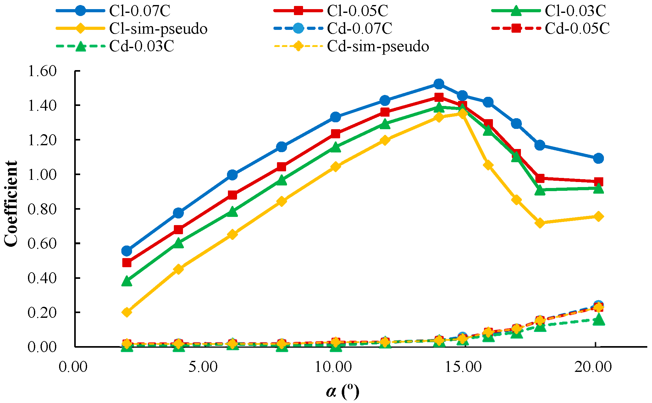
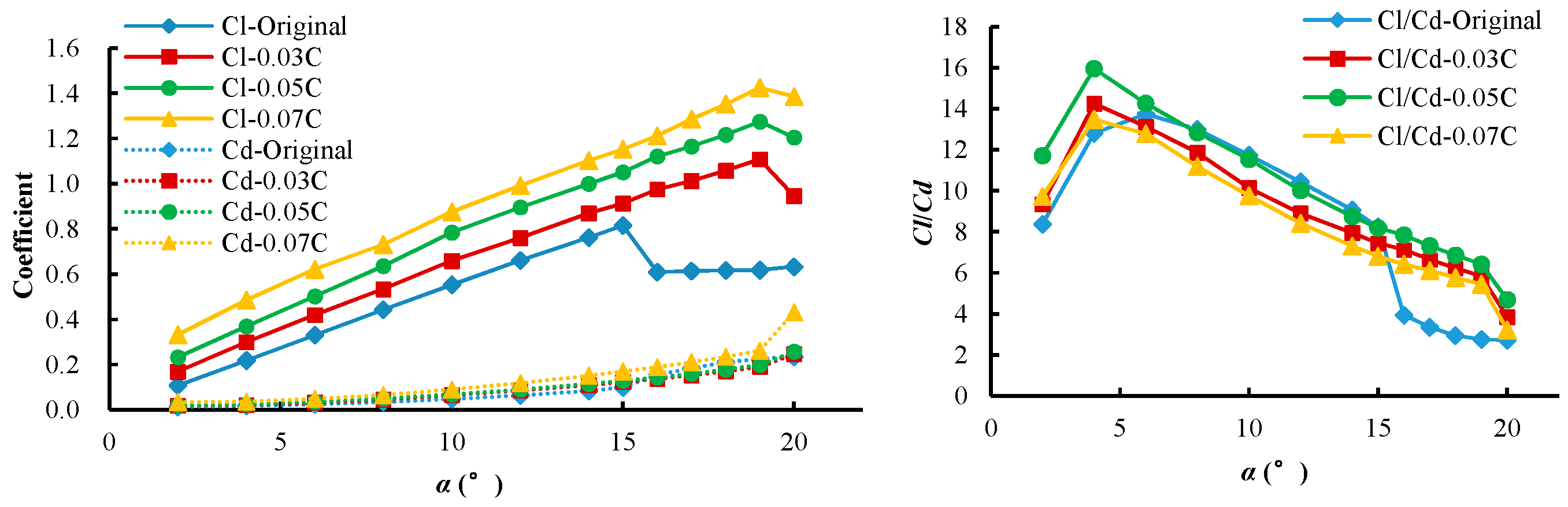
Firstly, with the increase of the angle of attack, for the pseudo 3D NACA0012 airfoil with the airfoil maximum deformation amplitude of 3%, 5% and 7% of the chord length, the lift coefficients firstly increase and then decrease. The lift coefficients of these deformed airfoils are all bigger than that of the original airfoil. At the same angle of attack, bigger the maximum deformation amplitude, higher the lift coefficient. The pseudo 3D NACA0012 airfoil reduces the scale of the surface vortex in some extend when compared with that of the deformed airfoil. When the maximum deformation amplitude reaches 0.05c, the best vortex controlling effect can be achieved and the airfoil demonstrates good aerodynamic performance.

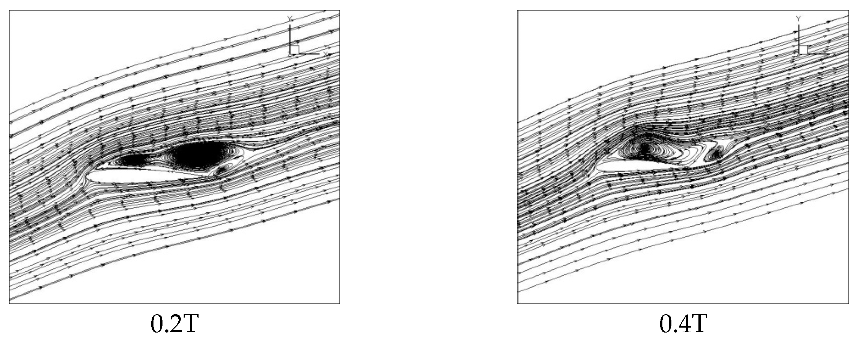
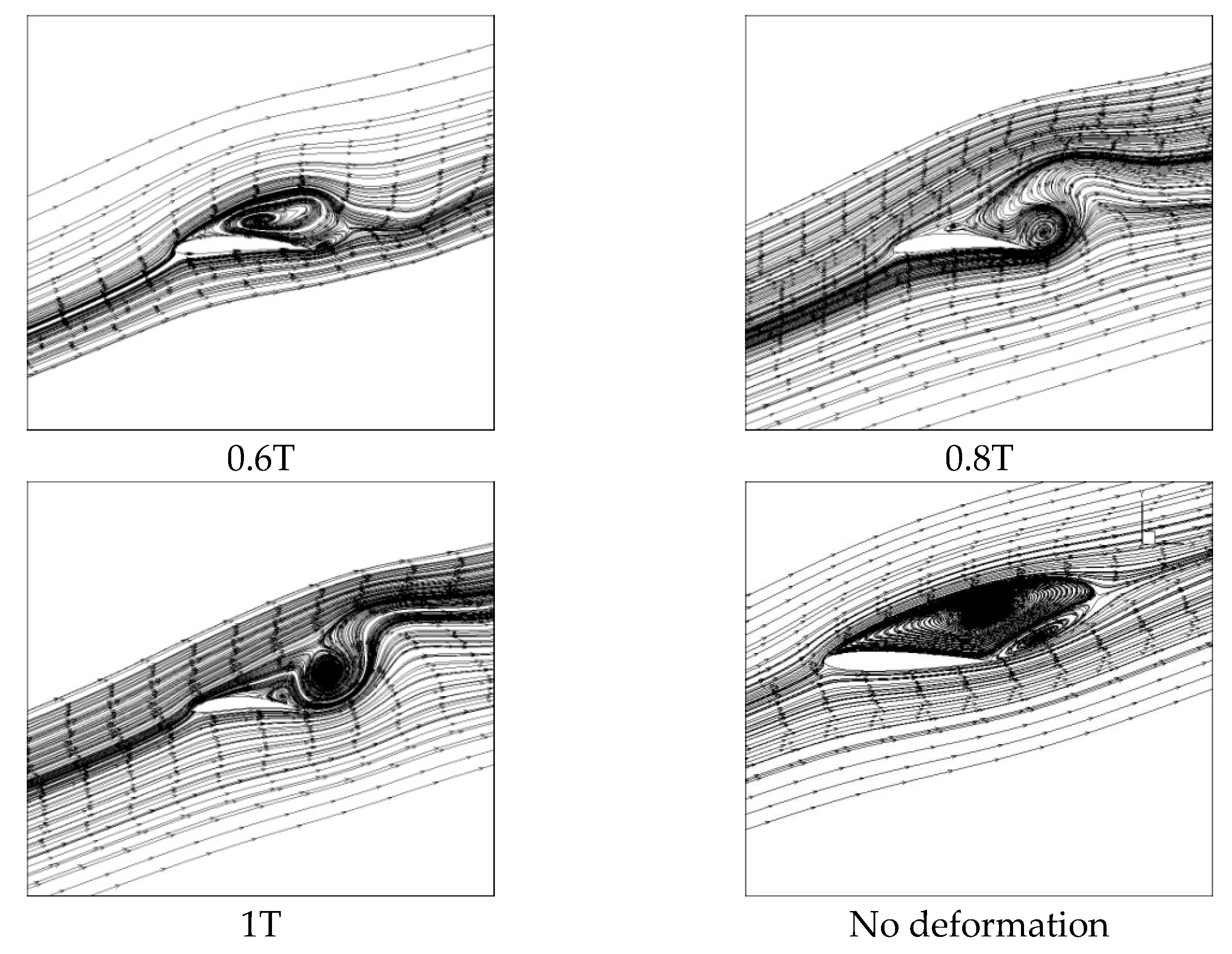
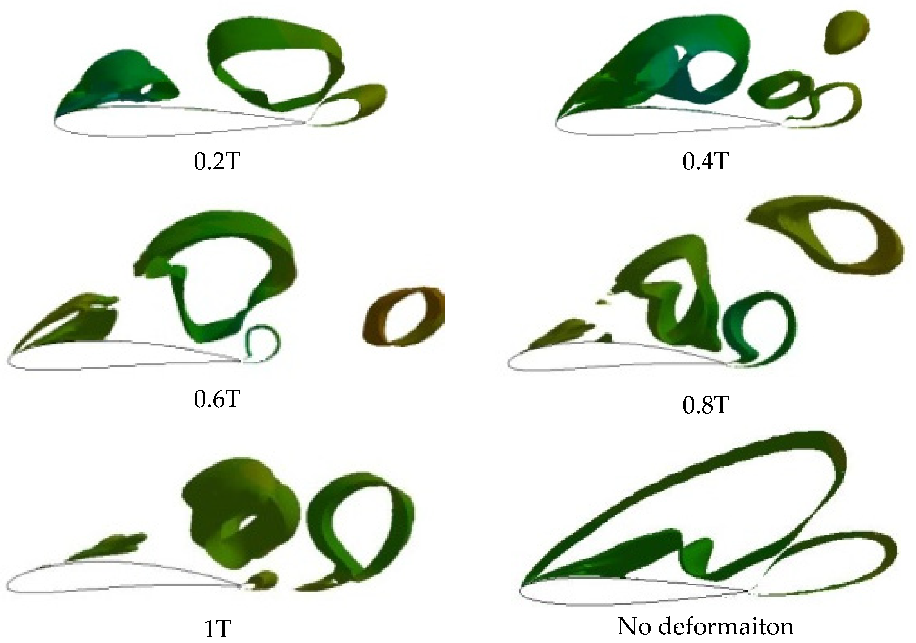
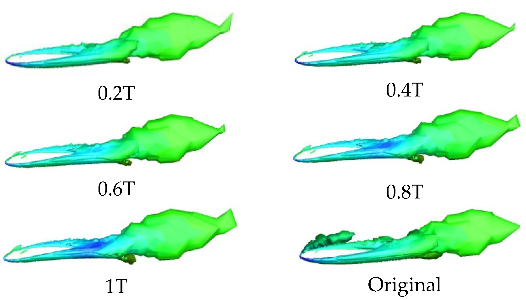
Secondly, with the increase of the angle of attack, the lift coefficients of the real 3D NACA0012 airfoil at the maximum deformation amplitude of 3%, 5% and 7% of chord length firstly increase and then decrease. All of these airfoils have a higher lift coefficient than the original airfoil. The 3D vortex figure demonstrates that the deformable airfoil has a better vortex generation controlling effect at the middle cross-section along the spanwise direction than the non-deformable airfoil.

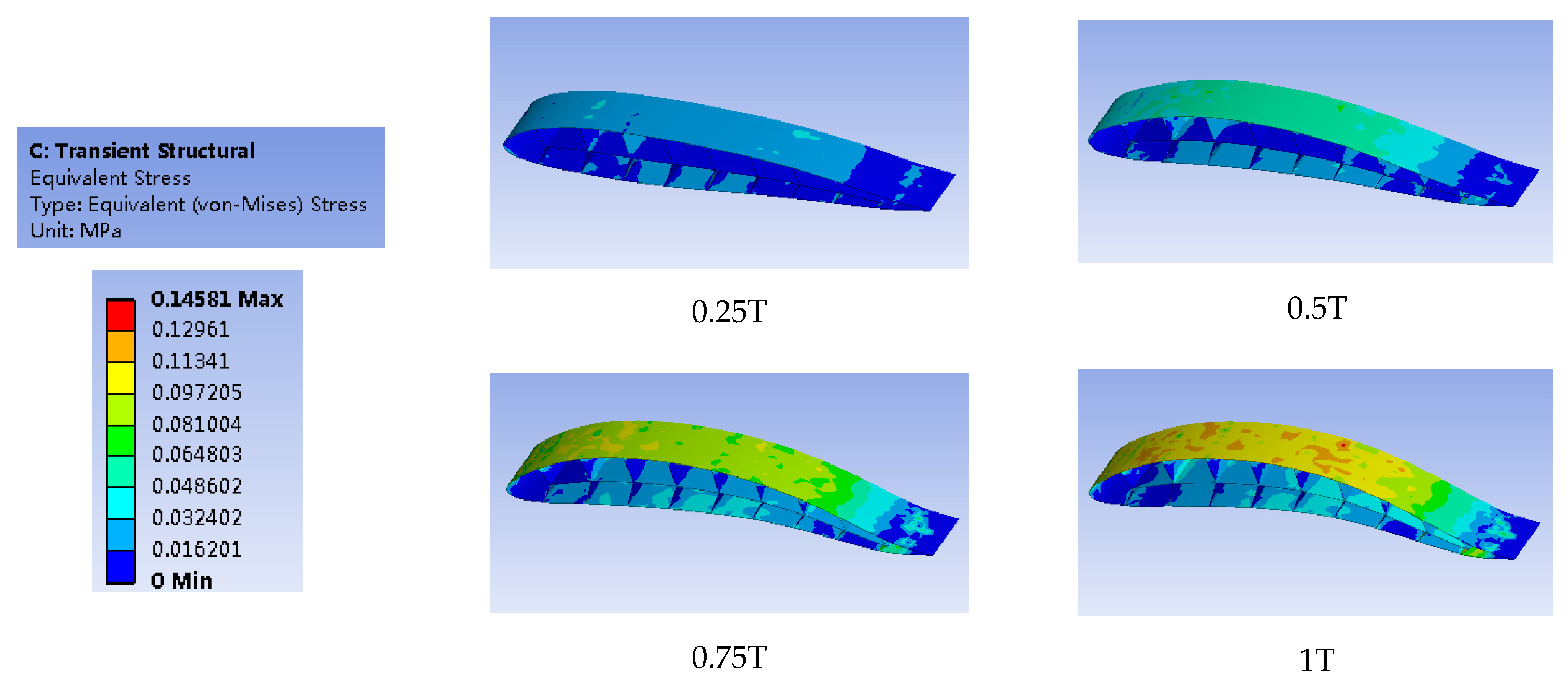
Thirdly, a new fish skeleton-like airfoil based on the NACA0012 airfoil has been proposed. At the angle of attack of 18°, the aerodynamic performance of the fish skeleton like airfoil with the Young’s modulus of 1 Mpa and 2 Mpa have been studied by using the fluid-solid coupling method. Results show that the passive deformation airfoil shares nearly the same characteristics as the active deformation airfoil. With a smaller Young’s modulus value, a smaller stress for the airfoil surface is tended to achieve, thus leading to a better aerodynamic performance. Therefore, this kind of new fish skeleton-like airfoil is expected to improve the aerodynamic performance of the VAWT and also augment its energy extraction efficiency performance.

References

1. Liu, Y.; Kokko, A. Wind power in China: Policy and development challenges. Energy Policy 2010, 38, 5520–5529. [Google Scholar] [CrossRef]
2. Muhammad, I.; Zhao, Z.Y.; Ahmad, M.; Mukeshimana, M.C. Critical factors influencing wind power industry: A diamond model based study of India. Energy Rep. 2019, 5, 1222–1235. [Google Scholar]
3. Boulouiha, H.M.; Allali, A.; Denai, M. Chapter Nine-Grid Integration of Wind Energy Systems: Control Design, Stability, and Power Quality Issues, Clean Energy for Sustainable Development; Academic Press: Cambridge, MA, USA, 2017; pp. 239–335. [Google Scholar]
4. Yanbing, C.; Zhi, L. The design of vertical axis wind turbine. Machinery 2012, 39, 36–39. [Google Scholar]
5. Okeoghene, E.; Louis, A.; Danao, M.; Robert, J.H. Experimental investigation of the influence of solidity on the performance and flow field aerodynamics of vertical axis wind turbines at low Reynolds numbers. Renew. Energy 2016, 92, 474–483. [Google Scholar]
6. Muhammad, M.; Nasir, H.; Ahmed, U.; Zain, A.; RehanJami, Z. Vertical axis wind turbine—A review of various configurations and design techniques. Renew. Sustain. Energy Rev. 2012, 16, 1926–1939. [Google Scholar]
7. Darrieus, G. Turbine Having its Rotating Shaft Transverse to Flow of Current. U.S. Patent 1834018, 8 December 1931. [Google Scholar]
8. Qing’an, L.; Takao, M.; Yasunari, K.; Junsuke, M.; Kazuma, F.; Masayuk, Y. Effect of number of blades on aerodynamic forces on a straight-bladed Vertical Axis Wind Turbine. Energy 2015, 90, 784–795. [Google Scholar]
9. Daynes, S.; Weaver, P.M. A shape adaptive airfoil for a wind turbine blade. In SPIE Smart Structures and Materials Nondestructive Evaluation and Health Monitoring; International Society for Optics and Photonics: San Diego, Ca, USA, 2011; p. 79790H. [Google Scholar]
10. Kerho, M. Adaptive airfoil dynamic stall control. J. Aircr. 2007, 44, 1350–1360. [Google Scholar] [CrossRef]
11. Capuzzi, M.; Pirrera, A.; Weaver, P.M. A novel adaptive blade concept for large-scale wind turbines. Part I: Aeroelastic behavior. Energy 2014, 73, 15–24. [Google Scholar] [CrossRef]
12. Hoogedoorn, E.; Jacobs, G.B.; Beyene, A. Aero-elastic behavior of a flexible blade for wind turbine application: A 2D computational study. Energy 2010, 35, 778–785. [Google Scholar] [CrossRef]
13. Jafaryar, M.; Kamrani, R.; Gorji-Bandpy, M.; Hatami, M.; Ganji, D.D. Numerical optimization of the asymmetric blades mounted on a vertical axis cross-flow wind turbine. Int. Commun. Heat Mass Transf. 2016, 70, 93–104. [Google Scholar] [CrossRef]
14. Menter, F.R. Two-equation eddy-viscosity turbulence models for engineering applications. AIAA J. 1994, 32, 1598–1605. [Google Scholar] [CrossRef] [Green Version]
15. McLaren, K.W. A Numerical and Experimental Study of Unsteady Loading of High-Solidity Vertical Axis Wind Turbines. Ph.D. Thesis, McMaster University, Hamilton, ON, Canada, 2011. [Google Scholar]
16. Ying, W.; Xiaojing, S.; Xiaohua, D.; Bing, Z.; Diangui, H.; Zhongquan, Z. Numerical investigation on aerodynamic performance of a novel vertical axis wind turbine with adaptive blades. Energy Convers. Manag. 2016, 108, 275–286. [Google Scholar]
17. Tong, H.; Fang, J.; Guo, J. Numerical Simulation of Unsteady Aerodynamic Performance of Novel Adaptive Airfoil for Vertical Axis Wind Turbine. Energies 2019, 12, 4106. [Google Scholar] [CrossRef] [Green Version]
18. Daróczy, L.; Gábor, J.; Klaus, P.; Michael, W.; Dominique, T. Comparative analysis of turbulence models for the aerodynamic simulation of H-Darrieus rotors. Energy 2015, 90, 680–690. [Google Scholar] [CrossRef]
19. Gosselin, R.; Dumas, G.; Boudreau, M. Parametric study of H-Darrieus vertical-axis turbines using uRANS simulations (Paper CFDSC-2013 178). In Proceedings of the 21st Annual Conference of the CFD Society of Canada, Sherbrooke, QC, Canada, 6–9 May 2013. [Google Scholar]
20. Marsh, P.; Ranmuthugala, D.; Penesis, I.; Thomas, G. Three-dimensional numerical simulations of straight-bladed vertical axis tidal turbines investigating power output, torque ripple and mounting forces. Renew Energy 2015, 83, 67–77. [Google Scholar] [CrossRef] [Green Version]
21. McNaughton, J.; Billard, F.; Revell, A. Turbulence modelling of low Reynolds number flow effects around a vertical axis turbine at a range of tip-speed ratios. J. Fluids Struct. 2014, 47, 124–138. [Google Scholar] [CrossRef]
22. Ladson, C.L. Effects of Independent Variation of Mach and Reynolds Numbers on the Low-Speed Aerodynamic Characteristics of the NACA 0012 Airfoil Section; NASA Scientific and Technical Information Division: Washington, DC, USA, 1988.
Figure 1. The technical scheme of the VAWT.
Energies 14 00880 g001
Figure 2. The airfoil deformation profile.
Energies 14 00880 g002
Figure 3. The Grid profile: (a) general mesh geometry for the whole flow field; (b) mesh distribution near the airfoil.
Energies 14 00880 g003
Figure 4. Comparison between the experiment of Ladson and our calculation results with mesh size of 457,600.
Energies 14 00880 g004
Figure 5. Geometry structure and mesh structure of the real 3D NACA0012 airfoil: (a) Geometry structure of the airfoil; (b) Mesh at the end part of the airfoil; (c) Mesh at the end part of the airfoil; (d) Airfoil circumferential grid distribution.
Energies 14 00880 g005
Figure 6. Different shapes of the airfoil skeleton models: (a) Skeleton model with three flat plant support in the chord line direction; (b) Skeleton model with flat plant support in both the chord line direction and camber line direction; (c) Skeleton model with solid material in the inner part of the airfoil; (d) Fish skeleton structure support airfoil.
Energies 14 00880 g006
Figure 7. Mesh structure of the airfoil: (a) The boundary condition of the solid zone; (b) The whole grid structure; (c) The airfoil circumferential grid distribution; (d) The grid distribution of the solid zone.
Energies 14 00880 g007
Figure 8. Comparison of the lift and drag coefficients of the NACA0012 airfoil between the maximum deformation amplitudes of 3%, 5% and 7% of chord length at the angles of attack of 0° to 20°.
Energies 14 00880 g008
Figure 9. Flow field and vortex demonstration for the pseudo 3D NACA0012 with the maximum deformation amplitude of 7% of chord length and the NACA0012 airfoil with non-deformation in one period (angle of attack of 19°).
Energies 14 00880 g009aEnergies 14 00880 g009b
Figure 10. Vortex demonstration for the pseudo 3D NACA0012 with the maximum deformation amplitude of 7% of chord length and the NACA0012 airfoil with non-deformation in one period (angle of attack of 19°).
Energies 14 00880 g010
Figure 11. Flow field and vortex demonstration for the pseudo 3D NACA0012 with the maximum deformation amplitude of 5% of chord length and the NACA0012 airfoil with non-deformation in one period (angle of attack of 19°).
Energies 14 00880 g011
Figure 12. Vortex demonstration for the pseudo 3D NACA0012 with the maximum deformation amplitude of 5% of chord length and the NACA0012 airfoil with non-deformation in one period (angle of attack of 19°).
Energies 14 00880 g012
Figure 13. Comparison of the lift and drag coefficients of the real 3D NACA0012 with the maximum deformation amplitudes of 3%, 5% and 7% of chord length at the angles of attack of 0° to 20°.
Energies 14 00880 g013
Figure 14. The fluid fields demonstration for different cross-sections along the airfoil spanwise direction (0.1B, 0.5B and 0.9B) at the angle of attack of 18° for the maximum deformation amplitude of 0.05c.
Energies 14 00880 g014aEnergies 14 00880 g014b
Figure 15. The demonstration of the vortex distribution for the middle cross-section of the airfoil along the spanwise direction with the maximum deformation amplitude of 0.05c.
Energies 14 00880 g015
Figure 16. Comparison of the flow fields between the airfoil with the Young’s Modulus of 2 Mpa and the original airfoil at the angle of attack of 18 ° .
Energies 14 00880 g016aEnergies 14 00880 g016b
Figure 17. Comparison of the surface pressure coefficient between the airfoil with the Young’s modulus of 2 Mpa and the original airfoil at the angle of attack of 18 ° .
Energies 14 00880 g017
Figure 18. Deformation shape of the fish skeleton airfoil in one cycle.
Energies 14 00880 g018
Figure 19. Deformation of the fish skeleton airfoil’s structure in one cycle with the Young’s modulus of 1 Mpa.
Energies 14 00880 g019
Figure 20. Deformation of the fish skeleton airfoil’s structure in one cycle with the Young’s Modulus of 2 Mpa.
Energies 14 00880 g020
Figure 21. Equal stress distribution of the fish skeleton airfoil with the Young’s modulus of 1 Mpa.
Energies 14 00880 g021
Figure 22. Equal stress distribution of the fish skeleton airfoil with the Young’s modulus of 2 Mpa.
Energies 14 00880 g022