
Extreme Wind and Waves in U.S. East Coast Offshore Wind Energy Lease Areas

 ,
, 
Abstract
1. Introduction
1.1. Background and Motivation
1.2. Research Objectives
2. Methods
2.1. ERA5
2.2. Annual Maximum and Extreme Wind Speeds
2.3. Annual Maximum and Extreme Wave Heights
2.4. Cyclone Genesis and Tracking
3. Results
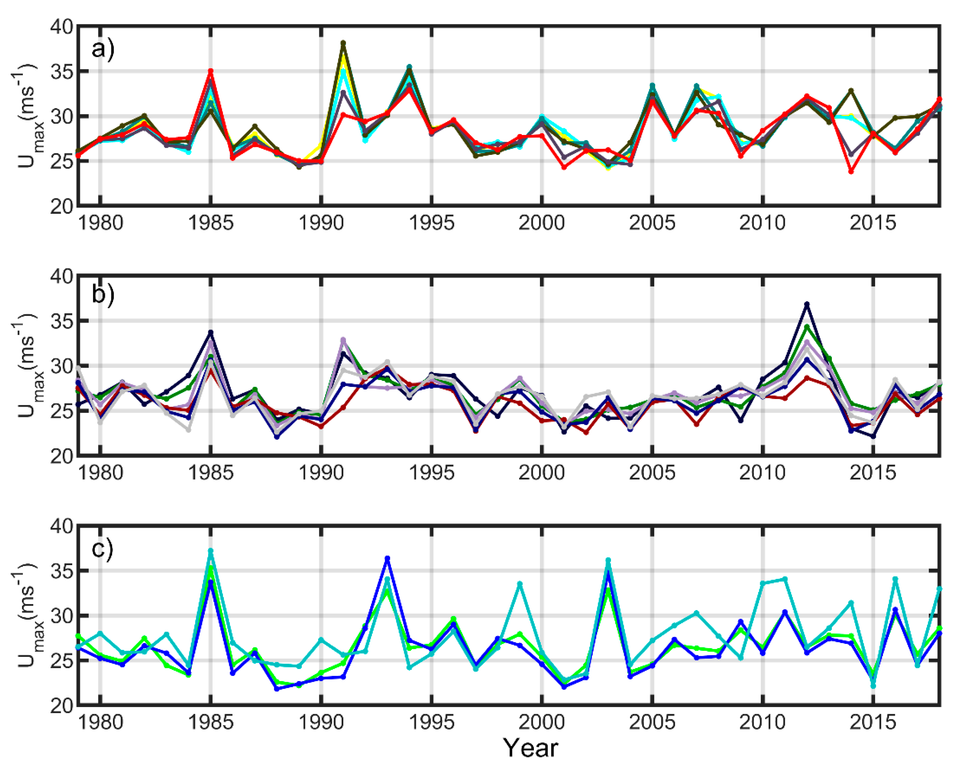
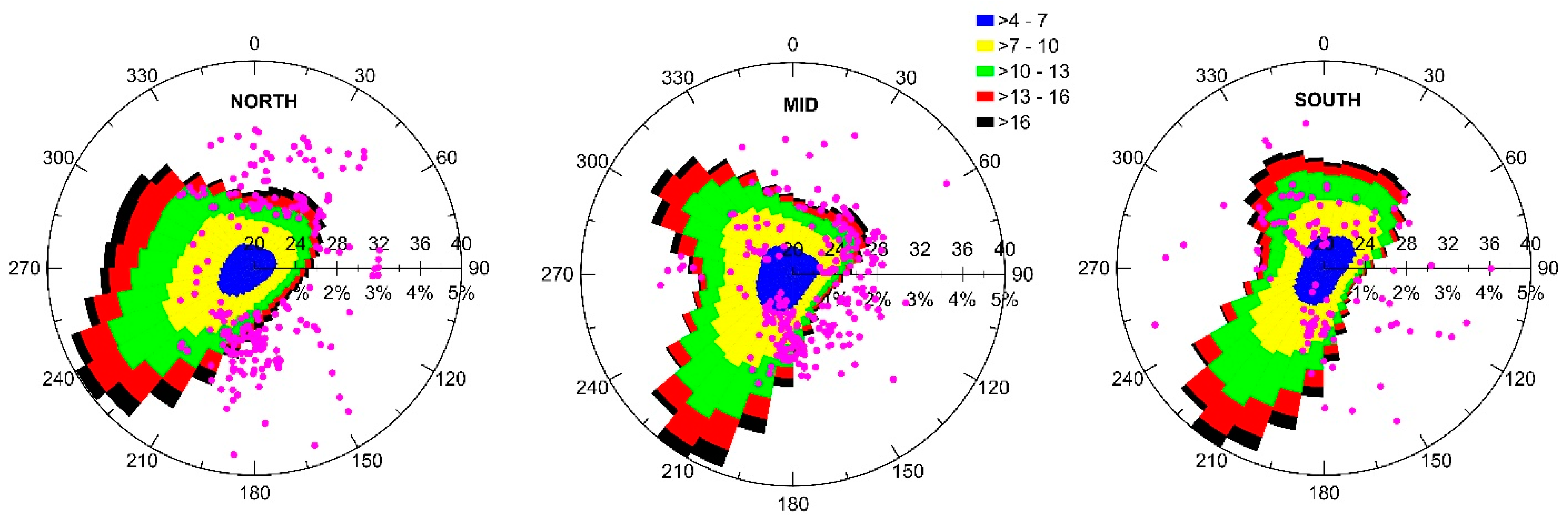
3.1. Wind Speeds
Annual Maximum Wind Speeds
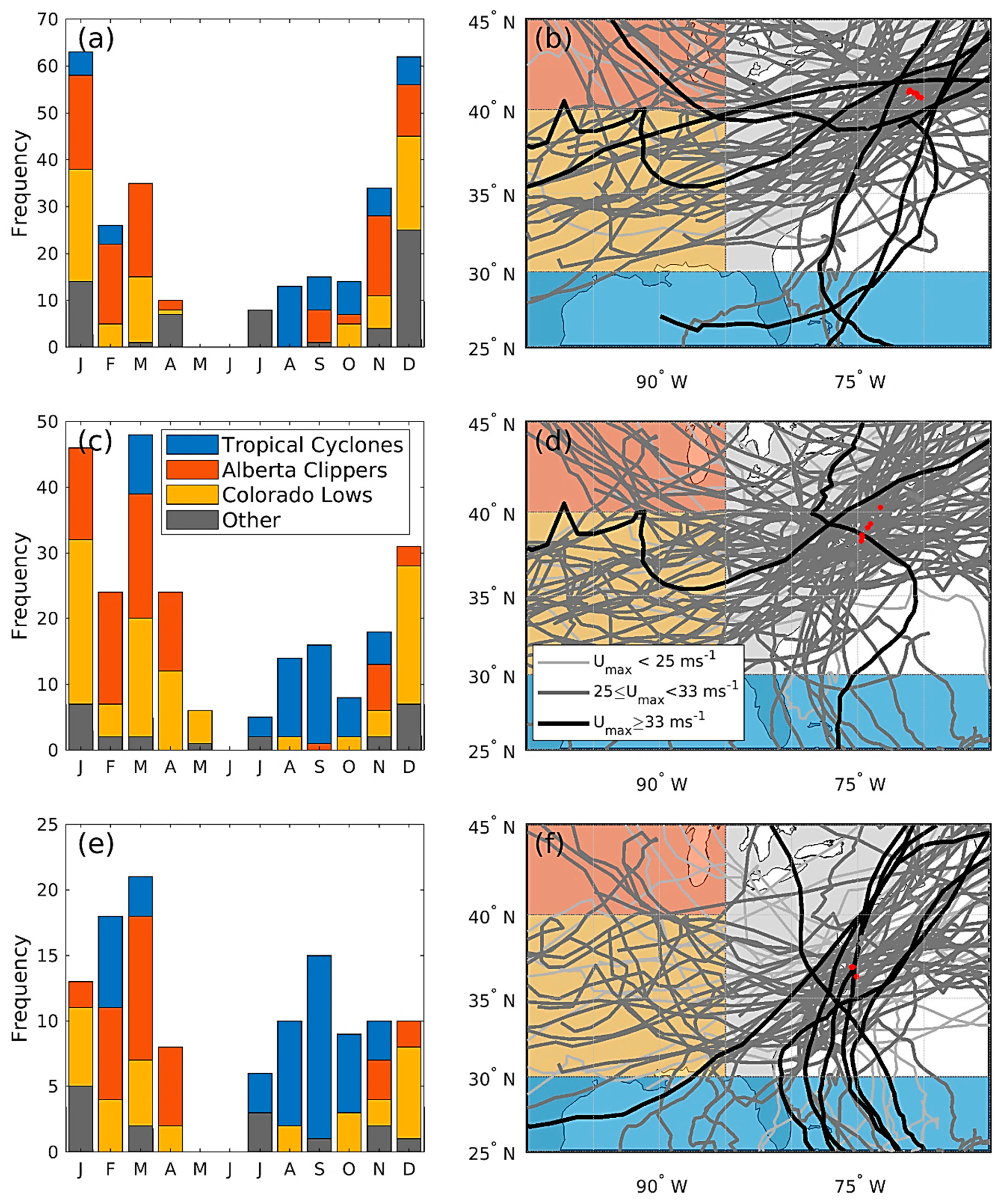
3.2. Sources of Intense and Extreme Wind Speeds
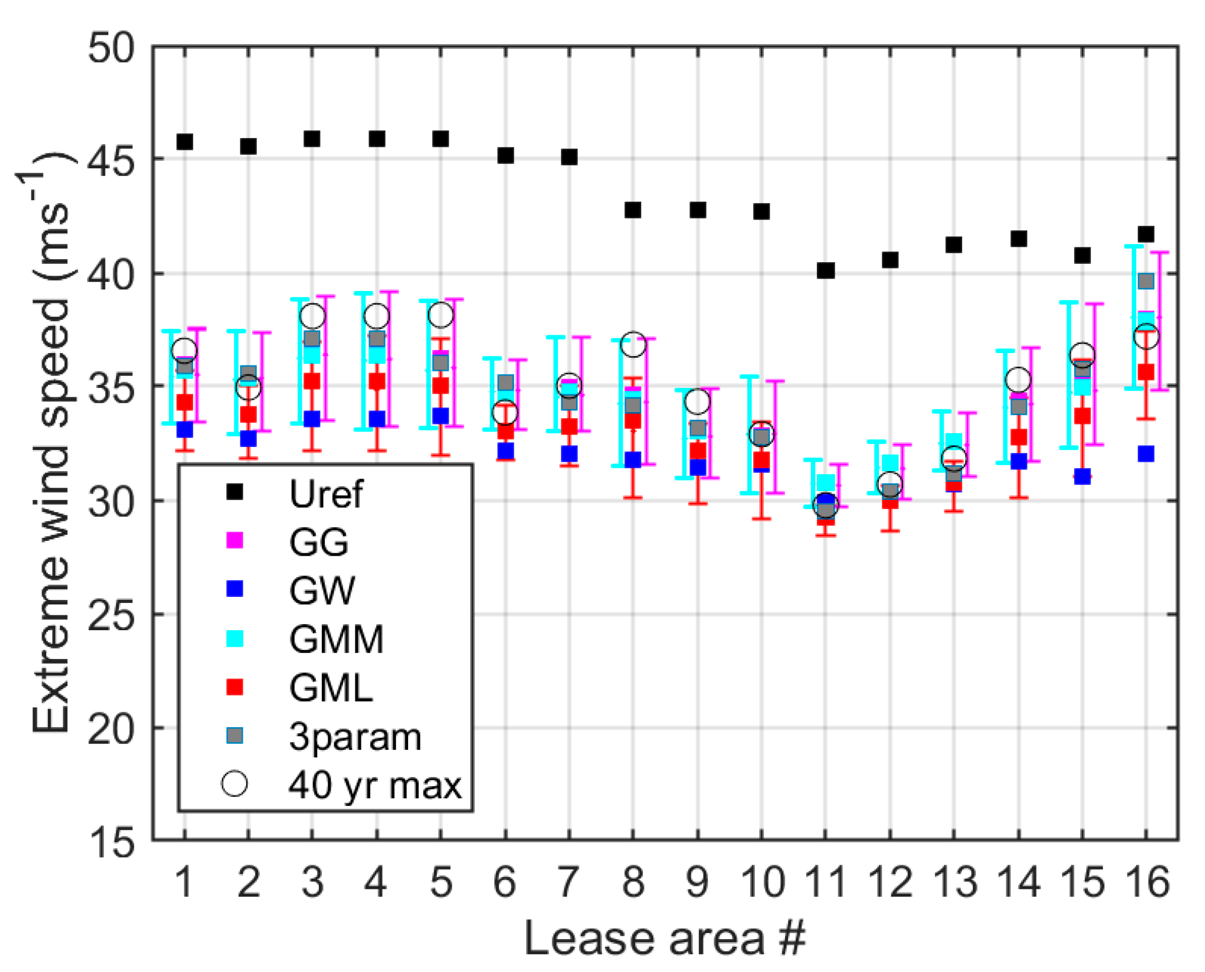
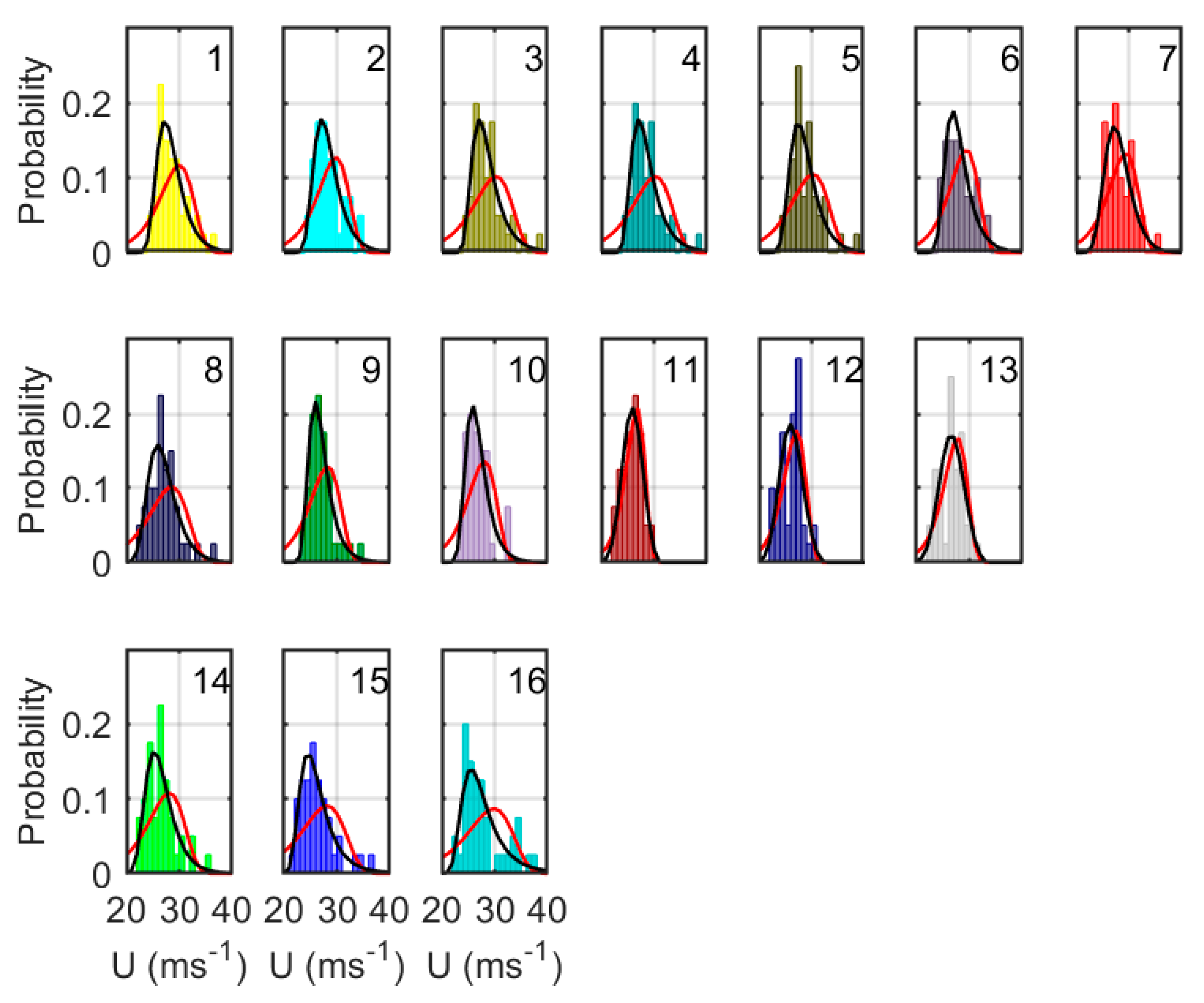
3.3. Results from the Different Methods of Estimating U50
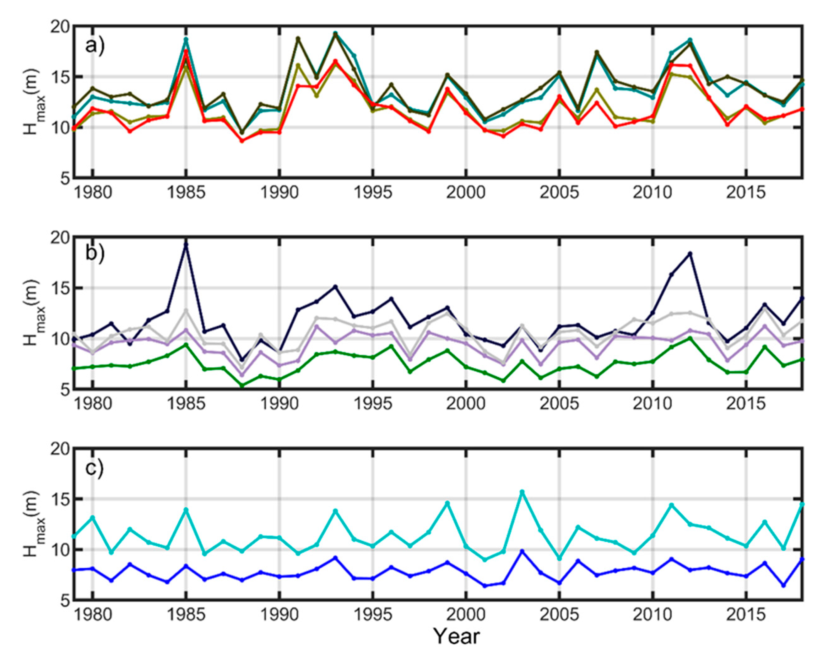
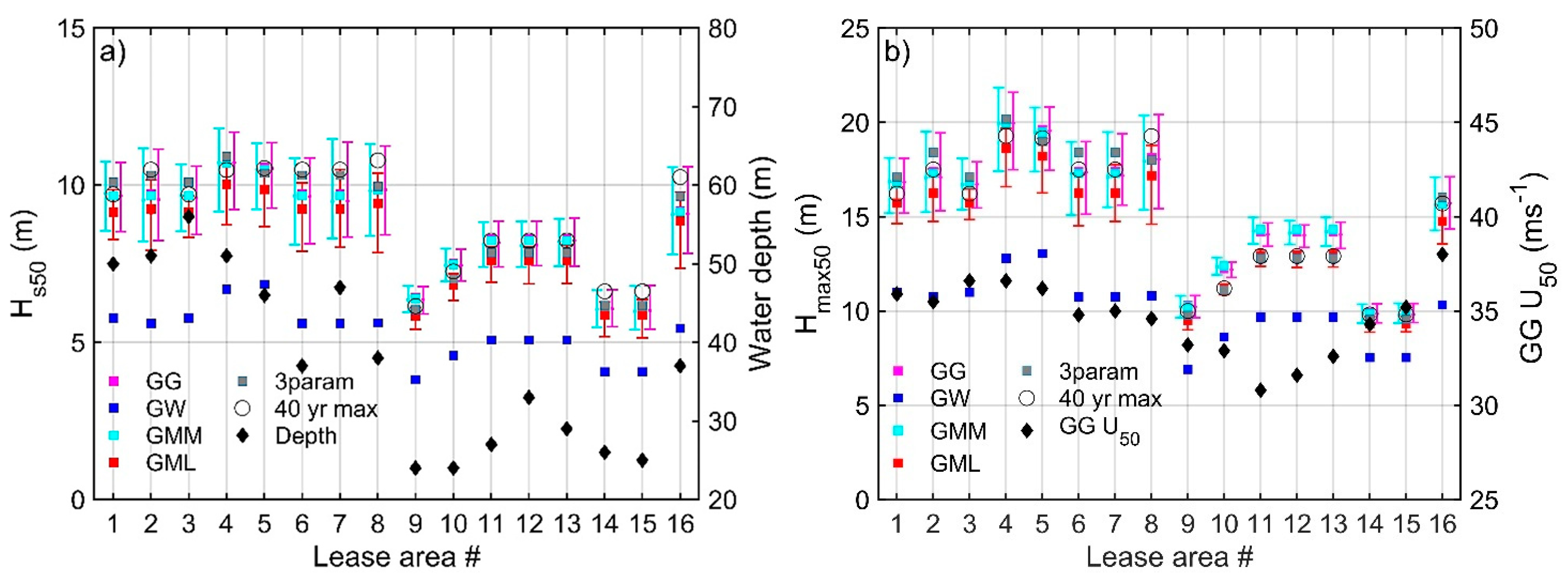
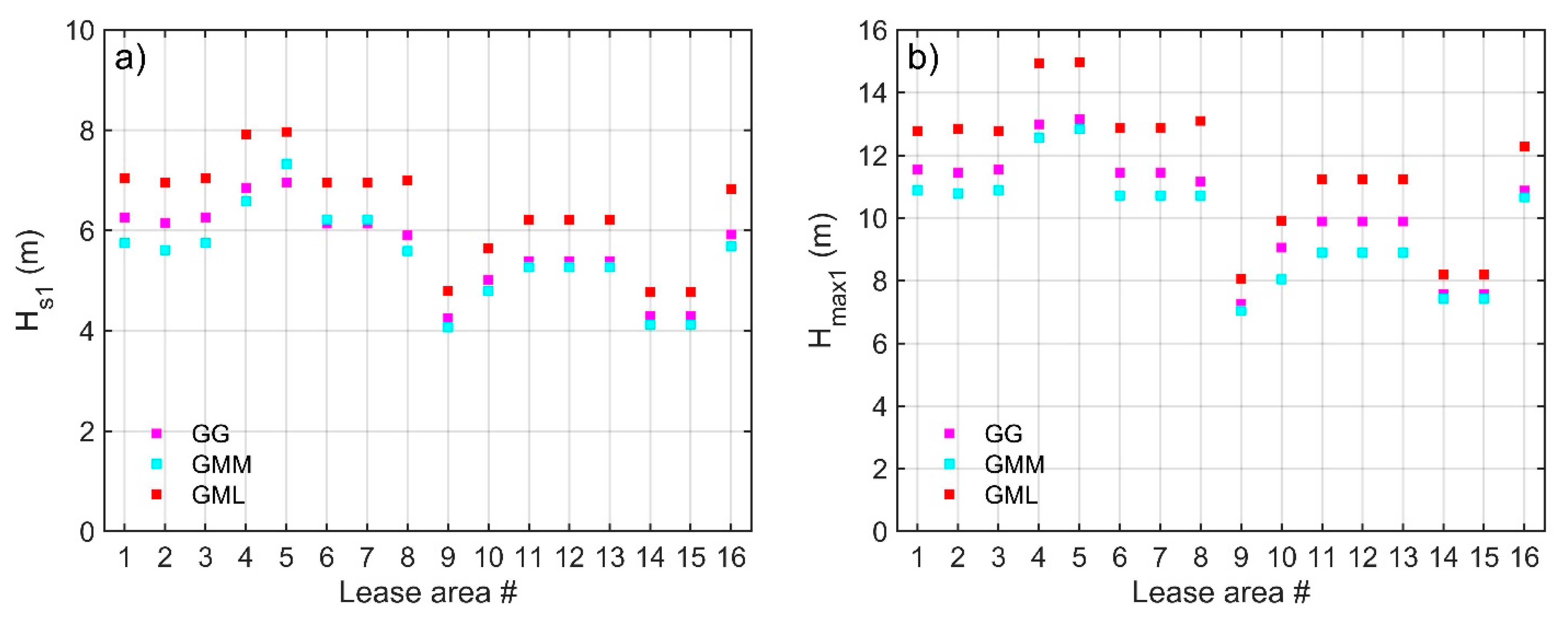
3.4. Wave Heights
4. Discussion
5. Concluding Remarks
Supplementary Materials
Author Contributions
Funding
Institutional Review Board Statement
Informed Consent Statement
Data Availability Statement
Acknowledgments
Conflicts of Interest
References
- WindEurope. Wind Energy in Europe Trends and Statistics 2019. 2020, p. 24. Available online: https://windeurope.org/wp-content/uploads/files/about-wind/statistics/WindEurope-Annual-Statistics-2019.pdf (accessed on 27 February 2020).
- Jansen, M.; Staffell, I.; Kitzing, L.; Quoilin, S.; Wiggelinkhuizen, E.; Bulder, B.; Riepin, I.; Müsgens, F. Offshore wind competitiveness in mature markets without subsidy. Nat. Energy 2020, 5, 614–622. [Google Scholar] [CrossRef]
- Bosch, J.; Staffell, I.; Hawkes, A.D. Global levelised cost of electricity from offshore wind. Energy 2019, 189, 116357. [Google Scholar] [CrossRef]
- WindEurope. Offshore Wind in Europe Key Trends and Statistics; 2020; p. 40. Available online: https://windeurope.org/wp-content/uploads/files/about-wind/statistics/WindEurope-Annual-Offshore-Statistics-2019.pdf (accessed on 27 February 2020).
- Musial, W.; Heimiller, D.; Beiter, P.; Scott, G.; Draxl, C. 2016 Offshore Wind Energy Resource Assessment for the United States. Technical Report NREL/TP-5000-66599. 2016; p. 88. Available online: https://www.nrel.gov/docs/fy16osti/66599.pdf (accessed on 16 July 2020).
- EIA. Electric Power Annual 2019 October 2020; US Energy Information Administration, 2020; p. 240. Available online: https://www.eia.gov/electricity/annual/pdf/epa.pdf (accessed on 22 November 2020).
- DeCastro, M.; Salvador, S.; Gómez-Gesteira, M.; Costoya, X.; Carvalho, D.; Sanz-Larruga, F.; Gimeno, L. Europe, China and the United States: Three different approaches to the development of offshore wind energy. Renew. Sustain. Energy Rev. 2019, 109, 55–70. [Google Scholar] [CrossRef]
- BOEM. Coastal Virginia Offshore Wind Project (CVOW). Available online: https://www.boem.gov/renewable-energy/state-activities/coastal-virginia-offshore-wind-project-cvow (accessed on 22 November 2020).
- AWEA. US Offshore Wind Energy Status Update OTOBER 2019. 2019. Available online: https://www.awea.org/Awea/media/Resources/Fact%20Sheets/Offshore-Fact-Sheet-Oct-2019.pdf (accessed on 22 July 2020).
- BOEM. BOEM Governing Statutes. Available online: https://www.boem.gov/about-boem/regulations-guidance/boem-governing-statutes (accessed on 15 October 2020).
- BOEM. 2020. Available online: https://www.boem.gov/sites/default/files/documents/renewable-energy/Renewable-Energy-OCS-Fact-Sheet.pdf (accessed on 22 July 2020).
- EIA. Electricity: Detailed State Data. 2020. Available online: https://www.eia.gov/electricity/data/state/ (accessed on 20 July 2020).
- Mills, A.D.; Millstein, D.; Jeong, S.; Lavin, L.; Wiser, R.; Bolinger, M. Estimating the value of offshore wind along the United States’ eastern coast. Environ. Res. Lett. 2018, 13, 094013. [Google Scholar] [CrossRef]
- BOEM. Outer Continental Shelf Renewable Energy Leases Map Book; 2019; p. 19. Available online: https://www.boem.gov/sites/default/files/renewable-energy-program/Mapping-and-Data/Renewable_Energy_Leases_Map_Book_March_2019.pdf (accessed on 22 July 2020).
- Barthelmie, R.J.; Pryor, S.C.; Frandsen, S.T. Climatological and meteorological aspects of predicting offshore wind energy. In Offshore Wind Energy; Twidell, J., Gaudiosi, G., Eds.; Multi-Science Publishing Co. Ltd.: Esses, UK, 2009; p. 425. ISBN 978-0906522639. [Google Scholar]
- Archer, C.L.; Colle, B.A.; Delle Monache, L.; Dvorak, M.J.; Lundquist, J.; Bailey, B.H.; Beaucage, P.; Churchfield, M.J.; Fitch, A.C.; Kosovic, B. Meteorology for coastal/offshore wind energy in the United States: Recommendations and research needs for the next 10 years. Bull. Am. Meteorol. Soc. 2014, 95, 515–519. [Google Scholar] [CrossRef]
- Ahsbahs, T.; Maclaurin, G.; Draxl, C.; Jackson, C.; Monaldo, F.; Badger, M. US East Coast synthetic aperture radar wind atlas for offshore wind energy. Wind Energy Sci. 2020, 5, 1191–1210. [Google Scholar] [CrossRef]
- Dvorak, M.J.; Corcoran, B.A.; Ten Hoeve, J.E.; McIntyre, N.G.; Jacobson, M.Z. US East Coast offshore wind energy resources and their relationship to peak-time electricity demand. Wind Energy 2013, 16, 977–997. [Google Scholar] [CrossRef]
- James, E.P.; Benjamin, S.G.; Marquis, M. Offshore wind speed estimates from a high-resolution rapidly updating numerical weather prediction model forecast dataset. Wind Energy 2018, 21, 264–284. [Google Scholar] [CrossRef]
- International Electrotechnical Commission. International Standard, IEC61400 Wind Turbines Wind Energy Generation Systems–Part 1: Design Requirements, Edition 4.0 2019-02; IEC, FDIS: Geneva, Switzerland, 2019; p. 172. [Google Scholar]
- International Electrotechnical Commission. International Standard, IEC61400 Wind Turbines Part 3-1: Design Requirements for Fixed Offshore Wind Turbines, Edition 1.0 2019-04; IEC, FDIS: Geneva, Switzerland, 2019; p. 314. [Google Scholar]
- Pryor, S.C.; Barthelmie, R.J. A global assessment of extreme wind speeds for wind energy applications. Nat. Energy 2021. Available online: https://www.nature.com/articles/s41560-020-00773-7 (accessed on 6 January 2021). [CrossRef]
- Wu, X.; Hu, Y.; Li, Y.; Yang, J.; Duan, L.; Wang, T.; Adcock, T.; Jiang, Z.; Gao, Z.; Lin, Z. Foundations of offshore wind turbines: A review. Renew. Sustain. Energy Rev. 2019, 104, 379–393. [Google Scholar] [CrossRef]
- Paulsen, B.T.; de Sonneville, B.; van der Meulen, M.; Jacobsen, N.G. Probability of wave slamming and the magnitude of slamming loads on offshore wind turbine foundations. Coast. Eng. 2019, 143, 76–95. [Google Scholar] [CrossRef]
- Holthuijsen, L.H.; Powell, M.D.; Pietrzak, J.D. Wind and waves in extreme hurricanes. J. Geophys. Res. Ocean. 2012, 117. [Google Scholar] [CrossRef]
- Rose, S.; Jaramillo, P.; Small, M.J.; Apt, J. Quantifying the hurricane catastrophe risk to offshore wind power. Risk Anal. 2013, 33, 2126–2141. [Google Scholar] [CrossRef]
- Rose, S.; Jaramillo, P.; Small, M.; Grossmann, D.; Apt, J. Quantifying the hurricane risk to offshore wind turbines. Proc. Natl. Acad. Sci. USA 2012. Available online: www.pnas.org/cgi/doi/10.1073/pnas.1111769109 (accessed on 20 November 2020). [CrossRef] [PubMed]
- Hallowell, S.T.; Myers, A.T.; Arwade, S.R.; Pang, W.; Rawal, P.; Hines, E.M.; Hajjar, J.F.; Qiao, C.; Valamanesh, V.; Wei, K. Hurricane risk assessment of offshore wind turbines. Renew. Energy 2018, 125, 234–249. [Google Scholar] [CrossRef]
- Landsea, C.W.; Franklin, J.L. Atlantic Hurricane Database Uncertainty and Presentation of a New Database Format. Mon. Weather Rev. 2013, 141, 3576–3592. [Google Scholar] [CrossRef]
- Jagger, T.H.; Elsner, J.B. Climatology Models for Extreme Hurricane Winds near the United States. J. Clim. 2006, 19, 3220. [Google Scholar] [CrossRef]
- Miller, J.E. Cyclogenesis in the Atlantic coastal region of the United States. J. Meteorol. 1946, 3, 31–44. [Google Scholar] [CrossRef]
- Marciano, C.G.; Lackmann, G.M.; Robinson, W.A. Changes in U.S. East Coast Cyclone Dynamics with Climate Change. J. Clim. 2015, 28, 468–484. [Google Scholar] [CrossRef]
- Gramcianinov, C.B.; Campos, R.M.; de Camargo, R.; Hodges, K.I.; Guedes Soares, C.; da Silva Dias, P.L. Analysis of Atlantic extratropical storm tracks characteristics in 41 years of ERA5 and CFSR/CFSv2 databases. Ocean Eng. 2020, 216, 108111. [Google Scholar] [CrossRef]
- Colle, B.A.; Booth, J.F.; Chang, E.K.M. A Review of Historical and Future Changes of Extratropical Cyclones and Associated Impacts Along the US East Coast. Curr. Clim. Chang. Rep. 2015, 1, 125–143. [Google Scholar] [CrossRef] [PubMed]
- Hersbach, H.; Bell, B.; Berrisford, P.; Hirahara, S.; Horányi, A.; Muñoz-Sabater, J.; Nicolas, J.; Peubey, C.; Radu, R.; Schepers, D.; et al. The ERA5 global reanalysis. Q. J. R. Meteorol. Soc. 2020, 146, 1999–2049. [Google Scholar] [CrossRef]
- Gelaro, R.; McCarty, W.; Suárez, M.J.; Todling, R.; Molod, A.; Takacs, L.; Randles, C.A.; Darmenov, A.; Bosilovich, M.G.; Reichle, R.; et al. The Modern-Era Retrospective Analysis for Research and Applications, Version 2 (MERRA-2). J. Clim. 2017, 30, 5419–5454. [Google Scholar] [CrossRef] [PubMed]
- Pryor, S.C.; Barthelmie, R.J.; Bukovsky, M.S.; Leung, L.R.; Sakaguchi, K. Climate change impacts on wind power generation. Nat. Rev. Earth Environ. 2020. [Google Scholar] [CrossRef]
- Henneman, K.; Guilleroy, A. ERA5: Data Documentation. Available online: https://confluence.ecmwf.int/display/CKB/ERA5%3A+data+documentation#ERA5:datadocumentation-Spatialgrid (accessed on 15 October 2020).
- Larsén, X.G.; Ott, S.; Badger, J.; Hahmann, A.N.; Mann, J. Recipes for correcting the impact of effective mesoscale resolution on the estimation of extreme winds. J. Appl. Meteorol. Climatol. 2012, 51, 521–533. [Google Scholar] [CrossRef]
- Larsen, X.G.; Mann, J. The effects of disjunct sampling and averaging time on maximum mean wind speeds. J. Wind Eng. Ind. Aerodyn. 2006, 94, 581–602. [Google Scholar] [CrossRef]
- Olauson, J. ERA5: The new champion of wind power modelling? Renew. Energy 2018, 126, 322–331. [Google Scholar] [CrossRef]
- Kalverla, P.C.; Duncan, J.B., Jr.; Steeneveld, G.J.; Holtslag, A.A.M. Low-level jets over the North Sea based on ERA5 and observations: Together they do better. Wind Energy Sci. 2019, 4, 193–209. [Google Scholar] [CrossRef]
- Jourdier, B. Evaluation of ERA5, MERRA-2, COSMO-REA6, NEWA and AROME to simulate wind power production over France. Adv. Sci. Res. 2020, 17, 63–77. [Google Scholar] [CrossRef]
- Pryor, S.C.; Letson, F.W.; Barthelmie, R.J. Variability in wind energy generation across the contiguous USA. J. Appl. Meteorol. Climatol. 2020, 59, 2021–2039. [Google Scholar] [CrossRef]
- Knoop, S.; Ramakrishnan, P.; Wijnant, I. Dutch Offshore Wind Atlas Validation against Cabauw Meteomast Wind Measurements. Energies 2020, 13, 6558. [Google Scholar] [CrossRef]
- Onea, F.; Ruiz, A.; Rusu, E. An Evaluation of the Wind Energy Resources along the Spanish Continental Nearshore. Energies 2020, 13, 3986. [Google Scholar] [CrossRef]
- Kumar, V.S.; Asok, A.B.; George, J.; Amrutha, M.M. Regional Study of Changes in Wind Power in the Indian Shelf Seas over the Last 40 Years. Energies 2020, 13, 2295. [Google Scholar] [CrossRef]
- Lindvall, J.; Svensson, G.; Caballero, R. The impact of changes in parameterizations of surface drag and vertical diffusion on the large-scale circulaton in the Community Atmosphere Model (CAM5). Clim. Dyn. 2017, 48, 3741–3758. [Google Scholar] [CrossRef]
- Muhammed Naseef, T.; Sanil Kumar, V. Climatology and trends of the Indian Ocean surface waves based on 39-year long ERA5 reanalysis data. Int. J. Climatol. 2020, 40, 979–1006. [Google Scholar] [CrossRef]
- Bruno, M.F.; Molfetta, M.G.; Totaro, V.; Mossa, M. Performance Assessment of ERA5 Wave Data in a Swell Dominated Region. J. Mar. Sci. Eng. 2020, 8, 214. [Google Scholar] [CrossRef]
- Hallgren, C.; Arnqvist, J.; Ivanell, S.; Körnich, H.; Vakkari, V.; Sahlée, E. Looking for an Offshore Low-Level Jet Champion among Recent Reanalyses: A Tight Race over the Baltic Sea. Energies 2020, 13, 3670. [Google Scholar] [CrossRef]
- Pryor, S.C.; Barthelmie, R.J.; Clausen, N.; Drews, M.; MacKellar, N.; Kjellström, E. Analyses of possible changes in intense and extreme wind speeds over northern Europe under climate change scenarios. Clim. Dyn. 2012, 38, 189–208. [Google Scholar] [CrossRef]
- Gomes, L.; Vickery, B.J. Extreme wind speeds in mixed wind climates. J. Wind Eng. Ind. Aerodyn. 1978, 2, 331–344. [Google Scholar] [CrossRef]
- Palutikof, J.P.; Brabson, B.B.; Lister, D.H.; Adcock, S.T. A review of methods to calculate extreme wind speeds. Meteorol. Appl. 1999, 6, 119–132. [Google Scholar] [CrossRef]
- Pryor, S.C.; Schoof, J.T.; Barthelmie, R.J. Empirical downscaling of wind speed probability distributions. J. Geophys. Res. 2005, 110. [Google Scholar] [CrossRef]
- Pryor, S.C.; Schoof, J.T. Importance of the SRES in projections of climate change impacts on near-surface wind regimes. Meteorol. Z. 2010, 19, 267–274. [Google Scholar] [CrossRef]
- Larsén, X.G.; Kruger, A. Application of the spectral correction method to reanalysis data in south Africa. J. Wind Eng. Ind. Aerodyn. 2014, 133, 110–122. [Google Scholar] [CrossRef]
- Pryor, S.C.; Barthelmie, R.J.; Schoof, J.T. The impact of non-stationarities in the climate system on the definition of ‘a normal wind year’: A case study from the Baltic. Int. J. Climatol. 2005, 25, 735–752. [Google Scholar] [CrossRef]
- Wilks, D.S. Statistical Methods in the Atmospheric Sciences, 3rd ed.; International Geophysics Series; Academic Press: San Diego, CA, USA, 2011; p. 676. [Google Scholar]
- Rueda, A.; Camus, P.; Mendez, F.J.; Tomas, A.; Luceno, A. An extreme value model for maximum wave heights based on weather types. J. Geophys. Res. Ocean. 2016, 121, 1262–1273. [Google Scholar] [CrossRef]
- Cook, N.J.; Harris, R.I.; Whiting, R. Extreme wind speeds in mixed climates revisited. J. Wind Eng. Ind. Aerodyn. 2003, 91, 403–422. [Google Scholar] [CrossRef]
- Ishihara, T.; Yamaguchi, A. Prediction of the extreme wind speed in the mixed climate region by using Monte Carlo simulation and measure-correlate-predict method. Wind Energy 2014, 2015, 171–186. [Google Scholar] [CrossRef]
- Mackay, E.; Johanning, L. Long-term distributions of individual wave and crest heights. Ocean Eng. 2018, 165, 164–183. [Google Scholar] [CrossRef]
- Vanem, E. Non-stationary extreme value models to account for trends and shifts in the extreme wave climate due to climate change. Appl. Ocean Res. 2015, 52, 201–211. [Google Scholar] [CrossRef]
- Viselli, A.M.; Forristall, G.; Pearce, B.R.; Dagher, H.J. Estimation of extreme wave and wind design parameters for offshore wind turbines in the Gulf of Maine using a POT method. Ocean Eng. 2015, 104, 649–658. [Google Scholar] [CrossRef]
- Hiles, C.E.; Robertson, B.; Buckham, B.J. Extreme wave statistical methods and implications for coastal analyses. Estuar. Coast. Shelf Sci. 2019, 223, 50–60. [Google Scholar] [CrossRef]
- Hodges, K.I.; Lee, R.W.; Bengtsson, L. A Comparison of Extratropical Cyclones in Recent Reanalyses ERA-Interim, NASA MERRA, NCEP CFSR, and JRA-25. J. Clim. 2011, 24, 4888–4906. [Google Scholar] [CrossRef]
- Letson, F.; Barthelmie, R.J.; Hodges, K.I.; Pryor, S.C. Windstorms in the Northeastern United States. Nat. Hazards Earth Syst. Sci. 2020. In Review. [Google Scholar]
- Bender, M.A.; Ross, R.J.; Tuleya, R.E.; Kurihara, Y. Improvements in tropical cyclone track and intensity forecasts using the GFDL initialization system. Mon. Weather Rev. 1993, 121, 2046–2061. [Google Scholar] [CrossRef]
- Wu, C.-C.; Emanuel, K.A. Potential vorticity diagnostics of hurricane movement. Part 1: A case study of Hurricane Bob (1991). Mon. Weather Rev. 1995, 123, 69–92. [Google Scholar] [CrossRef]
- Galarneau, T.J., Jr.; Davis, C.A.; Shapiro, M.A. Intensification of Hurricane Sandy (2012) through extratropical warm core seclusion. Mon. Weather Rev. 2013, 141, 4296–4321. [Google Scholar] [CrossRef]
- Cook, N.J. Confidence limits for extreme wind speeds in mixed climates. J. Wind Eng. Ind. Aerodyn. 2004, 92, 41–51. [Google Scholar] [CrossRef]
- Barthelmie, R.J.; Badger, J.; Pryor, S.C.; Hasager, C.B.; Christiansen, M.B.; Jørgensen, B.H. Wind speed gradients in the coastal offshore environment: Issues pertaining to design and development of large offshore wind farms. Wind Eng. 2007, 31, 369–382. [Google Scholar] [CrossRef]
- Barthelmie, R.J.; Pryor, S.C. Can satellite sampling of offshore wind speeds realistically represent wind speed distributions? J. Appl. Meteorol. 2003, 42, 83–94. [Google Scholar] [CrossRef]
- Ferreira, J.; Soares, C.G. Modelling bivariate distributions of significant wave height and mean wave period. Appl. Ocean Res. 2002, 24, 31–45. [Google Scholar] [CrossRef]
- Guedes Soares, C.; Henriques, A. Statistical uncertainty in long-term distributions of significant wave height. J. Offshore Mech. Arct. Eng. 1996, 118, 284–291. [Google Scholar] [CrossRef]
- Baarholm, G.S.; Haver, S.; Økland, O.D. Combining contours of significant wave height and peak period with platform response distributions for predicting design response. Mar. Struct. 2010, 23, 147–163. [Google Scholar] [CrossRef]
- Rohmer, J.; Louisor, J.; Le Cozannet, G.; Thao, S.; Naveau, N.; Bertin, X. Attribution of Extreme Wave Height Records along the North Atlantic Coasts Using Hindcast Data: Feasibility and Limitations. J. Coast. Res. 2020, 95, 1268–1272. [Google Scholar] [CrossRef]
- Menéndez, M.; Méndez, F.J.; Izaguirre, C.; Luceño, A.; Losada, I.J. The influence of seasonality on estimating return values of significant wave height. Coast. Eng. 2009, 56, 211–219. [Google Scholar] [CrossRef]
- Larsén, X.G.; Bolanos, R.; Du, J.; Kelly, M.C.; Kofoed-Hansen, H.; Larsen, S.E.; Karagali, I.; Badger, M.; Hahmann, A.N.; Imberger, M. Extreme Winds and Waves for Offshore Turbines: Coupling Atmosphere and Wave Modeling for Design and Operation in Coastal Zones; Final Report for ForskEL Project PSO-12020 X-WiWa; DTU Wind Energy E-0154: Roskilde, Denmark, 2007; p. 114. ISBN 978-87-93549-22-7. [Google Scholar]
- Gaertner, E.; Rinker, J.; Sethuraman, L.; Zahle, F.; Anderson, B.; Barter, G.E.; Abbas, N.J.; Meng, F.; Bortolotti, P.; Skrzypinski, W. IEA Wind TCP Task 37: Definition of the IEA 15-Megawatt Offshore Reference Wind Turbine; National Renewable Energy Lab.(NREL): Golden, CO, USA, 2020. Available online: https://www.nrel.gov/docs/fy20osti/76773.pdf (accessed on 20 November 2020).


| State | Abbreviation | Offshore Wind Gross Potential (GW) [5] | Offshore Wind Electricity Generation Potential (TWh/y) [5] | 2018 Electricity Generation from Wind GWh/year [12] | 2018 Total Electricity Generation TWh/year [12] | Current Electricity from Onshore Wind [6] (% of Total Generation) | Potential Contribution to Electricity from Offshore Wind (% of Current Generation) |
|---|---|---|---|---|---|---|---|
| Connecticut | CT | 4.6 | 17 | 12.2 | 39.4 | 0.0 | 43.1 |
| Delaware | DE | 9.1 | 37.9 | 5.2 | 6.2 | 0.1 | 611.3 |
| Maine | ME | 127.5 | 645.9 | 2284.3 | 11.3 | 20.2 | 5715.9 |
| Maryland | MD | 130.8 | 603.2 | 570 | 43.8 | 1.3 | 1377.2 |
| Massachusetts | MA | 545.8 | 2858.1 | 221 | 27.2 | 0.8 | 10507.7 |
| New Hampshire | NH | 2.1 | 9.4 | 0.4 | 17.1 | 0.0 | 55.0 |
| New Jersey | NJ | 165.5 | 796.2 | 22.5 | 75 | 0.0 | 1061.6 |
| New York | NY | 165.6 | 786.1 | 3998.3 | 132.5 | 3.0 | 593.3 |
| North Carolina | NC | 807.4 | 3661.3 | 549.8 | 134.3 | 0.4 | 2726.2 |
| Pennsylvania | PA | 5.7 | 24.3 | 3566.9 | 215.4 | 1.7 | 11.3 |
| Rhode Island | RI | 21.3 | 103.1 | 158.6 | 8.4 | 1.9 | 1227.4 |
| Virginia | VI | 93.3 | 404.5 | 172.8 | 95.5 | 0.2 | 423.6 |
| Sum of all 12 states | 2078.7 | 9947.0 | 11,562.0 | 806.1 | 1.4 | 1234.0 | |
| US Total | 10,799.9 | 44,378.2 | 272,667.0 | 4178.0 | 7.1 | 1062.2 |
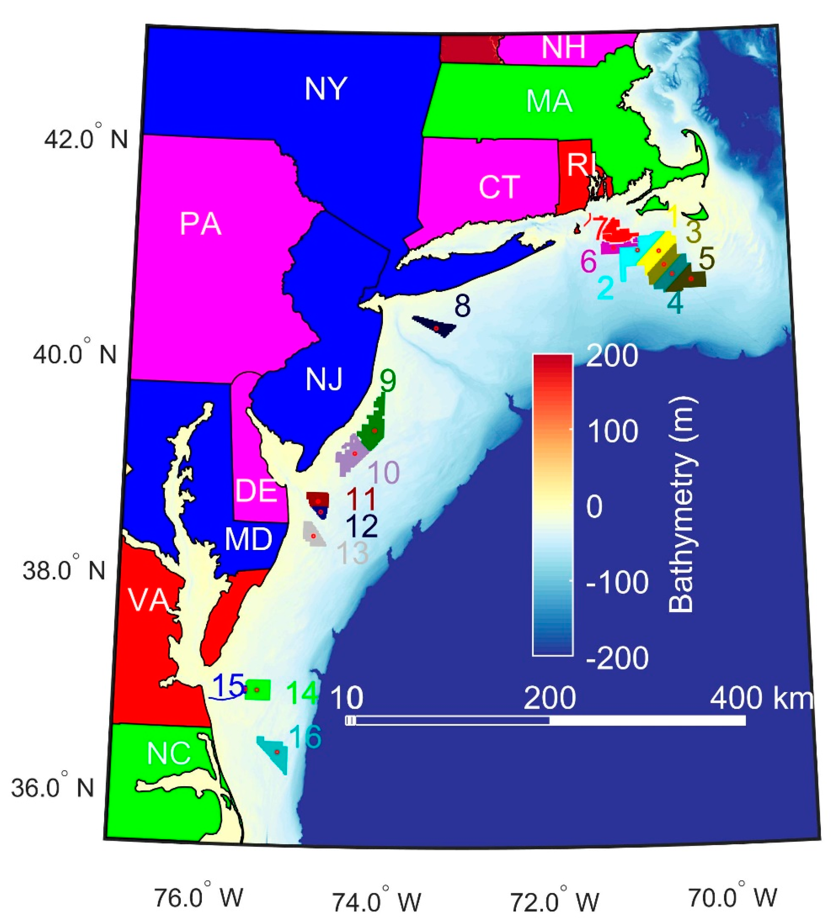
| Group | LA # | Lessee | State | Area (km2) | Identifier | Year Issued | Center Latitude (N) | Center Longitude (W) | Water Depth (m) | Distance to Coast (km) | Mean Annual Mean Wind Speed (ms−1) |
|---|---|---|---|---|---|---|---|---|---|---|---|
| North | 1 † | Vineyard Wind | MA | 675.7 | OCS-A 0501 | 2015 | 40.967 | 70.581 | 50 | 35 | 9.16 |
| 2 | Bay State Wind | MA | 759.2 | OCS-A 0500 | 2015 | 40.978 | 70.842 | 51 | 30 | 9.12 | |
| 3 *,† | Equinor | MA | 521.5 | OCS-A 0520 | 2018 | 40.839 | 70.522 | 56 | 53 | 9.17 | |
| 4 * | Mayflower Wind | MA | 515.7 | OCS-A 0521 | 2018 | 40.75 | 70.426 | 51 | 61 | 9.17 | |
| 5 | Vineyard Wind | MA | 535.9 | OCS-A 0522 | 2018 | 40.696 | 70.196 | 46 | 65 | 9.17 | |
| 6 ‡ | Deepwater Wind New England | RI/MA | 272.3 | OCS-A 0487 | 2013 | 41.119 | 71.075 | 37 | 26 | 9.02 | |
| 7 ‡ | Deepwater Wind New England | RI/MA | 394.7 | OCS-A 0486 | 2013 | 41.006 | 71.136 | 47 | 31 | 9.01 | |
| Mid | 8 | Equinor | NY | 321.3 | OCS-A 0512 | 2017 | 40.274 | 73.315 | 38 | 45 | 8.55 |
| 9 | Atlantic Shores Offshore Wind | NJ | 742.3 | OCS-A 0499 | 2016 | 39.321 | 74.046 | 24 | 31 | 8.55 | |
| 10 | Ocean Wind | NJ | 649.7 | OCS-A 0498 | 2016 | 39.106 | 74.279 | 24 | 32 | 8.54 | |
| 11 # | Garden State Offshore Energy I | DE | 283.8 | OCS-A 0482 | 2012 | 38.658 | 74.704 | 27 | 31 | 8.02 | |
| 12 # | Skipjack | DE | 106.6 | OCS-A 0519 | 2018 | 38.561 | 74.671 | 33 | 38 | 8.11 | |
| 13 # | US Wind | MD | 322.7 | OCS-A 0490 | 2014 | 38.337 | 74.750 | 29 | 28 | 8.24 | |
| South | 14 ^ | Virginia Electric and Power Company | VA | 456.7 | OCS-A 0483 | 2013 | 36.907 | 75.361 | 26 | 52 | 8.30 |
| 15 ^ | Virginia, Dept Mines, Min. Energy (Research) | VA | 8.6 | OCS-A 0497 | 2015 | 36.911 | 75.495 | 25 | 42 | 8.15 | |
| 16 | Avangrid Renewables | NC | 495.6 | OCS-A 0508 | 2017 | 36.342 | 75.108 | 37 | 58 | 8.34 |
| Method | Description | Description | References |
|---|---|---|---|
| Uref | (5) | Method used in IEC standards to derive a reference 50-year return period wind speed at hub-height | [20] |
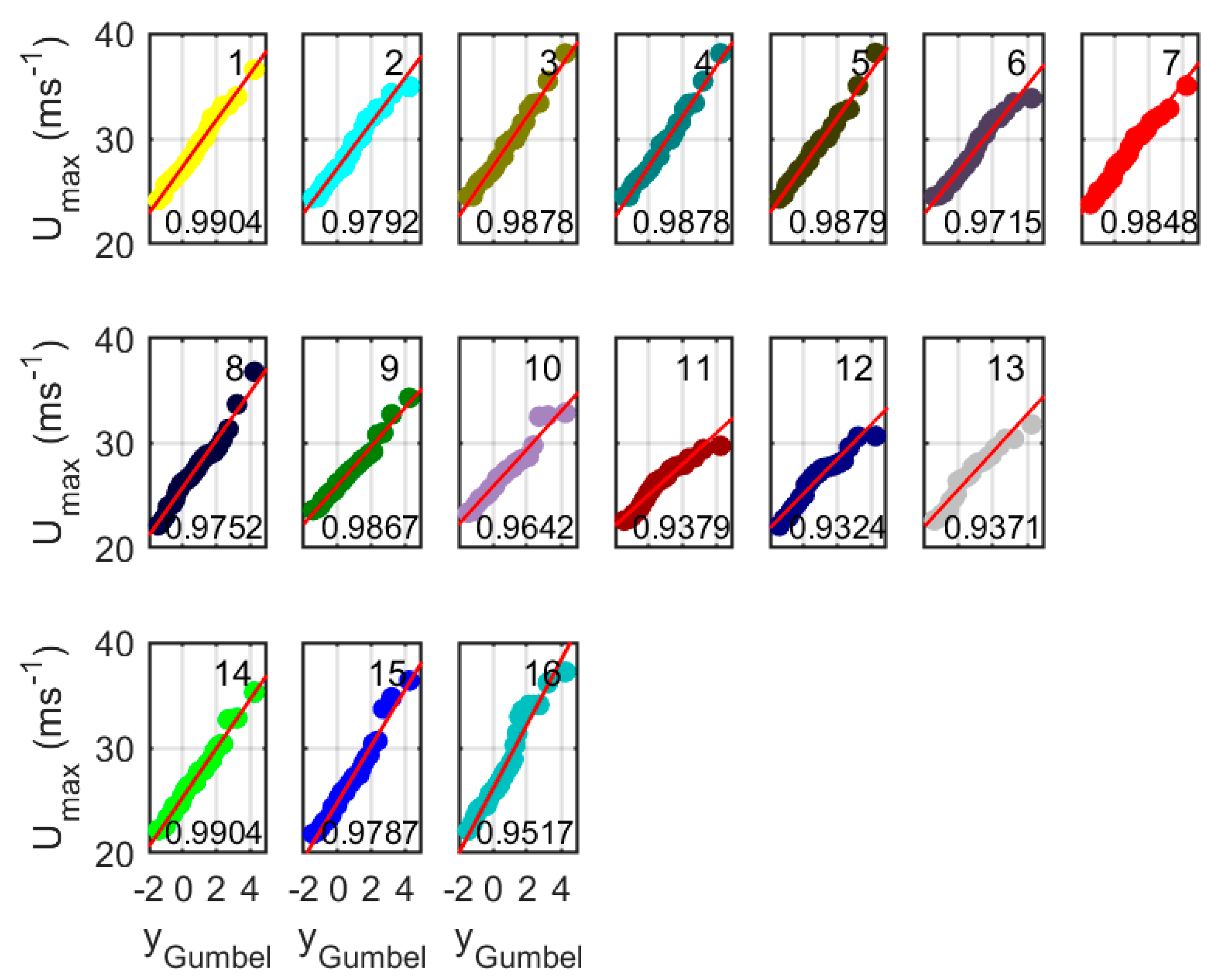
| Gumbel-graphical (GG) | (7) | Samples of annual maximum wind speed (Umax) are ranked and plotted against the reduced variate yGumbel (where m is the rank order position and N is the total sample size) and are subject to linear fitting using the least squares method to derive the slope and intercept (β and μ). In the absence of a mixed climate for extreme wind speeds [52,53], this relationship is linear. | [54] |
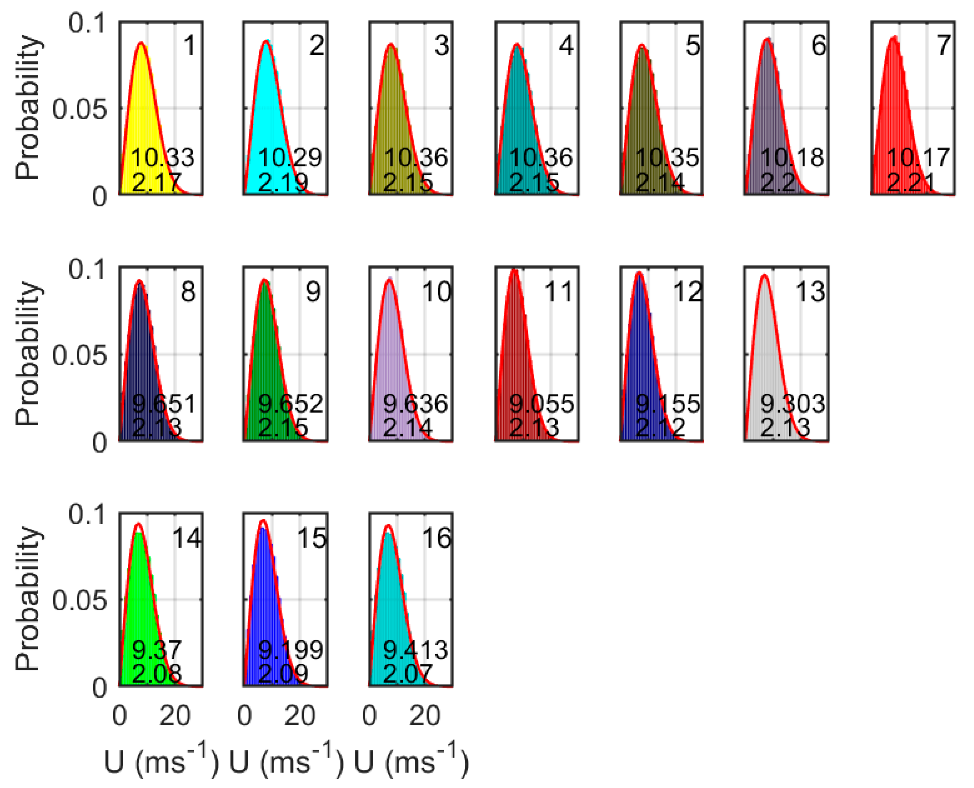
| Gumbel-Weibull (GW) | (8) (9) (10) | Wind speed (U) time series typically fit the two-parameter Weibull distribution [55,56] with scale parameter c and shape parameter k (Equation (8)) derived here using maximum likelihood methods. The resulting Weibull distribution parameters are linked to the Gumbel parameters using Equations (9) and (10). Note: nind is the number of independent observations (i.e., effective sample size approximated here using the lag-1 autocorrelation (r1) as where n’ is the sample size). While this method does not require multiple decades of data to obtain a good fit to the Weibull distribution, the fitting of the tail of the distribution is vulnerable to under-sampling of intense wind speeds. | [56] |
| Gumbel Method of Moments (GMM) | (12) (13) γ = Euler’s constant (0.577216) | The mean () and standard deviation (σ) of the samples of annual maximum wind speed (Umax) are used to derive the Gumbel distribution parameters (μ and β) following Equations (12) and (13). This method is fully analytical and uncertainty for the values of UT calculated using this method can be found using the addition of the third and fourth moments. | [57] |
| Gumbel Maximum Likelihood (GML) | Approach is implemented using fitdist in Matlab. | Maximum likelihood estimation methods (with iteration) are used to derive μ and β from the samples of annual maximum wind speed (Umax). This is a more computationally demanding but is a non-parametric approach. | [58] |
| Three parameter GEV with ML | Approach is implemented using fitdist in Matlab. | Maximum likelihood estimation methods (with iteration) are used to derive the 3 parameters in Equation (1) from samples of Umax. | [51] |
| LA | Hs | Hmax | Co-Occurrence of Maximum Hmax and Umax | ||||||
|---|---|---|---|---|---|---|---|---|---|
| Method⇒ | GG | GMM | GML | GG | GMM | GML | ±1.5 day | ±3 h | Top 3 ± 1.5 day |
| 1&3 | 6.26 | 5.75 | 7.04 | 11.55 | 10.88 | 12.78 | 58,58 | 53,53 | 54,55 |
| 2 | 6.15 | 5.61 | 6.95 | 11.44 | 10.78 | 12.85 | 65 | 58 | 56 |
| 4 | 6.85 | 6.58 | 7.92 | 12.99 | 12.55 | 14.94 | 48 | 45 | 53 |
| 5 | 6.96 | 7.32 | 7.97 | 13.16 | 12.85 | 14.97 | 40 | 38 | 48 |
| 6&7 | 6.14 | 6.21 | 6.95 | 11.44 | 10.71 | 12.86 | 65,65 | 60,60 | 54,55 |
| 8 | 5.90 | 5.59 | 7.00 | 11.15 | 10.71 | 13.10 | 40 | 38 | 44 |
| 9 | 4.25 | 4.07 | 4.79 | 7.26 | 7.04 | 8.06 | 48 | 48 | 48 |
| 10 | 5.01 | 4.80 | 5.64 | 9.05 | 8.04 | 9.92 | 38 | 33 | 43 |
| 11,12,13 | 5.39 | 5.27 | 6.21 | 9.89 | 8.89 | 11.23 | 40,48,53 | 33,40,45 | 43,44,49 |
| 14&15 | 4.30 | 4.13 | 4.77 | 7.57 | 7.43 | 8.20 | 50,50 | 50,48 | 52,54 |
| 16 | 5.92 | 5.68 | 6.83 | 10.87 | 10.66 | 12.27 | 63 | 55 | 56 |
Publisher’s Note: MDPI stays neutral with regard to jurisdictional claims in published maps and institutional affiliations. |
© 2021 by the authors. Licensee MDPI, Basel, Switzerland. This article is an open access article distributed under the terms and conditions of the Creative Commons Attribution (CC BY) license (http://creativecommons.org/licenses/by/4.0/).
Share and Cite
Barthelmie, R.J.; Dantuono, K.E.; Renner, E.J.; Letson, F.L.; Pryor, S.C. Extreme Wind and Waves in U.S. East Coast Offshore Wind Energy Lease Areas. Energies 2021, 14, 1053. https://doi.org/10.3390/en14041053
Barthelmie RJ, Dantuono KE, Renner EJ, Letson FL, Pryor SC. Extreme Wind and Waves in U.S. East Coast Offshore Wind Energy Lease Areas. Energies. 2021; 14(4):1053. https://doi.org/10.3390/en14041053
Chicago/Turabian StyleBarthelmie, Rebecca J., Kaitlyn E. Dantuono, Emma J. Renner, Frederick L. Letson, and Sara C. Pryor. 2021. "Extreme Wind and Waves in U.S. East Coast Offshore Wind Energy Lease Areas" Energies 14, no. 4: 1053. https://doi.org/10.3390/en14041053
APA StyleBarthelmie, R. J., Dantuono, K. E., Renner, E. J., Letson, F. L., & Pryor, S. C. (2021). Extreme Wind and Waves in U.S. East Coast Offshore Wind Energy Lease Areas. Energies, 14(4), 1053. https://doi.org/10.3390/en14041053