Abstract
We present an easily accessible model for dispatch and expansion planning of the German multi-modal energy system from today until 2050. The model can be used with low efforts while comparing favorably with historic data and other studies of future developments. More specifically, the model is based on a linear programming partial equilibrium framework and uses a compact set of technologies to ease the comprehension for new modelers. It contains all equations and parameters needed, with the data sources and model assumptions documented in detail. All code and data are openly accessible and usable. The model can reproduce today’s energy mix and its CO2 emissions with deviations below 10%. The generated energy transition path, for an 80% CO2 reduction scenario until 2050, is consistent with leading studies on this topic. Our work thus summarizes the key insights of previous works and can serve as a validated and ready-to-use platform for other modelers to examine additional hypotheses.
1. Introduction
The transition towards climate-friendly, reliable, and affordable energy systems requires deep transformations and the European Commission’s recent “Fit for 55 Package” exemplifies how this requires policy-making on a wide range of topics. Energy system modeling is a valuable support to prepare for such progress, since it enables the integrated analysis of multiple technical and economic aspects of the energy transition. Three major studies based on detailed quantitative models describe possible paths for the German energy system: the “Integrated Energy Transition” study commissioned by dena [1], “Climate Paths For Germany” by BDI [2], and “Energy Systems of the Future” by acatech ESYS [3].
Due to their high economic and political relevance, the call for transparency and accessibility of energy system models becomes ever stronger [4,5]. Several efforts have been made in this direction [6,7]. However, we still see major shortcomings which motivates this contribution.
Different approaches to energy system modeling are possible [8] and various frameworks are openly available, see the links listed by the Open Energy Modelling Initiative [9] and the Open Energy Platform [10]. Frameworks containing the mathematical equations of the common partial equilibrium models [11] include MARKAL [12,13], EFOM [14], TIMES [15], and more recently OSeMOSYS [16], Calliope [17], and oemof [18]. All of these models are open-source by now. “Ready-to-use” tools should, however, also include the data sets needed to parameterize the equations [7]. Only then can the results be reproduced. In this sense, complete model instances exist openly for test cases and a few countries such as South Africa [19], the United Kingdom [20], or the United States [21]. While for Germany many individual data pieces are openly available, e.g., data made available on the transparency platform operated by the European Network of Transmission System Operators for Electricity (ENTSO-E) [22] or data linked on the aforementioned online platforms, no comprehensive data model exists in the open domain.
Another barrier to easy access is the often very complex technology structure of the models. The MARKAL model, initially launched in the late 70s, was continuously developed and uses over 100 parameter types to study the costs and benefits of alternative energy scenarios in the future [13]. The European Union’s METIS model [23] has more than 60 different asset types that can be used to model a technology. While detail may be required to examine specific effects, such model complexity requires significant learning time from new modelers. Moreover, it also hinders the models’ explainability to decisionmakers, who are often not experts in the field [24]. Another line of thought against such detailed modeling is that it implicitly assumes that precise forecasting of future price, demand, and technology developments is possible. Such an assumption is rather questionable, e.g., considering that the price for crude oil changed abruptly by more than 50% from 2014 to 2016 and similar changes are hard to predict in the future.
Third, validation results for open energy system models are rarely available. One exception is [25] which reported back-testing results of their model against historic data from previous years. Such consistency with the past is mandatory to deliver trustworthy predictions.
This work addresses the three aforementioned shortcomings by providing a complete, compact, and validated model for the German energy transition. The model is a partial equilibrium model formulated as a linear programming (LP) optimization problem. It contains both the equations and the required data sets to model the German energy system from today until 2050. The entire source code and data are openly available (https://github.com/OCGModel/OCGModel accessed on 30 November 2021). We assume a very compact technology structure to reduce the complexity and thus enhance accessibility. When compared to historic data from 2016, the model replicates with deviations below 10%, important performance measures such as the use of primary energy sources, the electricity generation mix, and the aggregated CO2 emissions. We also benchmark the model’s projections about the future against the aforementioned studies of the German energy transition [1,2,3]. We find that our model results are within the predicted range of these studies.
The remainder of the paper structures as follows: Section 2 contains the model equations, describes the used technology setup, and reviews the sources of all parameter values. An openly accessible and usable implementation of the model based on a slightly adapted version of the Open Source Energy Modelling System (OSeMOSYS) framework is presented in Section 3. In Section 4 we validate the model results against historic data from 2016 and the forenamed three studies of future developments until 2050 [1,2,3]. We conclude in Section 5.
2. The Model
The proposed model is described in three steps. First, the mathematical formulation is described in Section 2.1. We use an abstract notation, and yet flexible, that allows us to describe all model equations very compactly. In Section 2.2, the structure of our compact technology map is introduced and explained. Finally, the sources and assumptions for all model parameters are explained in detail in Section 2.3. The actual parameter values are contained in an easy-to-read Excel file within the code repository.
2.1. Mathematical Formulation
The mathematical formulation of the model relies on two types of entities to characterize energy systems: commodities c represent different energy carriers, e.g., gas, coal, or electricity; conversion processes p describe the transformation of one energy commodity into another, e.g., a gas power plant transforms gas into electricity.
All commodities are treated model-endogenously except one special commodity named exogenous. Model-endogenous commodities are fully supplied and consumed within the model domain. The commodity is an abstraction used to describe all energy forms outside the model boundaries. The commodity can be consumed or supplied, but no conservation law holds for it.
Concerning conversion processes, we distinguish three different types as exemplified in Figure 1:
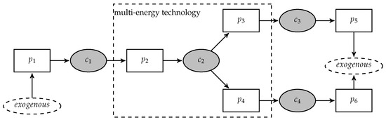
Figure 1.
Model abstraction for representing multi-energy systems. Rectangles represent the conversion processes, gray ellipses the model’s endogenous energy carriers (commodities), and white ellipses the special commodity. Each process has only one input and one output, multi-energy technologies as represented by the dashed rectangle can be modeled by linking several processes via auxiliary commodities.
- is an input process, adding energy to the system from energy,
- , , and are regular conversion processes that transform one model-endogenous commodity into another one,
- and are demand processes, transforming the endogenous energies and into energy.
Multi-energy technologies that consume and supply multiple energy forms, e.g., Combined Heat and Power (CHP) plants, can be modeled as shown by the dashed rectangle in Figure 1. In this case, is introduced as an auxiliary energy form, that couples the conversion processes , , and each representing different parts of a multi-energy technology. In the following, we will no longer draw the commodity in technology maps.
With this abstraction, the model is formulated compactly. It takes the form of an LP optimization problem whose equations are described in six content-related groups: (i) objective function, (ii) emissions constraints, (iii) aggregated variable definitions, (iv) energy and power balances, (v) operational constraints, and (vi) multi-year capacity constraints. Lower case symbols denote parameters while upper case symbols denote variables. Superscripts complement the parameter/variable description and subscripts refer to indices. An extended notation of a process is , making its specific input and output commodities explicit. Here, and are both aliases for c. The model covers several years y and time slices t within each such year. Concerning energy transport, the model considers a single region, the so-called copperplate assumption. This implies that no energy transport restrictions apply.
2.1.1. Objective Function
The optimization objective is the minimization of the discounted total system costs . These costs are composed of the investment, fixed operation & maintenance (O&M), and variable O&M costs of each conversion process, defined via the specific cost parameters , , and , respectively. Let , , and be the additionally built capacity, the active capacity, and the annual energy output of a conversion process p in the year y. The total costs of the system are then given as
where the discount factor to the financial base year , is calculated from the global discounting rate finatial discount rate r as .
2.1.2. Emissions Constraints
The CO2 emissions are accounted for by the energy output of each conversion process. The sum over all specific emissions over one year y yields the total annual CO2 emissions ,
If an upper limit is defined for the CO2 emission in year y, we add the following equation to the model,
2.1.3. Aggregated Variables
Different aggregated energy variables support a more comprehensive model formulation. Let and be the power in- and output of process p in year y and time slice t, respectively. The total energy output/input of the process in a year / is then,
where is the time slice t weight. The total power supply/consumption / of commodity c in time slice t of year y is defined as
2.1.4. Energy and Power Balance Constraints
Energy or power balance constraints are defined for model-endogenous commodities. For many commodities c the supplied power has to match the consumed power at every time slice t,
For commodities that can be stored at such relatively low cost that the corresponding storage processes are not relevant for the modeling, e.g., solid fuels such as coal, the aforementioned constraint is replaced by the annual energy balance
Note that apart from this implicit storage assumption we do not consider other storage types. Nevertheless, we can reproduce both today’s as well as projected energy systems as shown in the experimental section below.
2.1.5. Operational Constraints
For all processes, it holds that the power in- and output are coupled via the efficiency parameter ,
and that the power output is limited by the active capacity and the technical availability factor ,
Here, defines the usable share of the active capacity which may be lower than one, e.g., due to maintenance downtimes. When not stated explicitly, the efficiency and technical of 1 are assumed. For variable renewable energy (VRE), such as solar photovoltaics (PV) and wind turbines, we include the weather effects via the time-dependent availability factors and the condition
For some processes, especially demands which are modeled as a conversion process to the exogenous commodity, yearly minimal and maximum energy output parameters are defined. It then holds that
The temporal distribution of the output over the time slices, e.g., the normalized load profile of demands, can be specified via the distribution factors . These factors are defined such that and it then holds that
Limiting the relative power a process can consume of its input commodity is helpful to model multi-energy processes, e.g., CHP plants. Using the minimal and maximal input fractions we request that
The relative power that a process can contribute to its output commodity is treated in parallel,
where are the minimal and maximal fractions.
2.1.6. Capacity Constraints
We define the residual capacity for any process p as the capacity in the year y that remains available from construction times before the modeled period. The active capacity in year y is the sum of the residual capacity and the newly built capacity within the model,
with being a process’ technical lifetime. Lower and upper capacity limits can be defined for the active capacity to express technical potentials or legal restrictions for each technology,
2.2. Structure of the Technology Map
To model the German energy system we use the commodities and conversion processes described in the following. An aggregated representation of the resulting technology map is shown in Figure 2. Four groups of commodities are linked with seven groups of conversion processes.
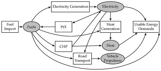
Figure 2.
Aggregated technology map of our model. Rectangles denote groups of conversion processes and ellipses represent groups of commodities.
2.2.1. Commodities
The model’s commodities can be categorized into four groups. They are listed group-wise in Table 1.

Table 1.
Commodity groups of our model with the contained individual energy forms.
Fuels
The fuel commodities of our model are mostly used to generate other energy forms, while also some direct demands exist. The fuels may come from fossil or renewable sources. All liquid hydrocarbons such as gasoline, diesel, or methanol are summarized into the commodity Liquid Fuel since their usage scenarios are relatively similar. One exception is crude oil, which is modeled separately to account for conversion losses during refining. Biomass includes also renewable waste, whereas Waste refers only to non-renewable waste.
Electricity
The model only considers one form of electricity and does not distinguish by location or voltage level. This is possible due to the assumption that intra-regional transport and voltage adaption are universally available through the power grid at high efficiency and comparably low cost.
Heat
In contrast, heat is separated by location and temperature. We distinguish between industrial zones and the decentral locations of buildings. A district heating grid may connect the two, but is not always available. We also separate temperature levels for industrial heat, since largely different technologies are required to supply one regime or another. Moreover, direct heat conversion is only possible from high to low temperatures due to the second law of thermodynamics. These arguments lead to three modeled heat commodities:
- Decentral Heat (DH): heat for space and water heating in buildings of the residential and commerce sectors,
- Low-Temperature Industrial Heat (LTIH): heat for low-temperature processes (<500 °C) in the industrial sector, e.g., paper production and to supply district heating systems,
- High-Temperature Industrial Heat (HTIH): heat for high-temperature processes (>500 °C) in the industrial sector, e.g., steel or glass production and various processes in the chemical industry.
Vehicle Propulsion
The commodity Vehicle Propulsion represents the mechanical energy required to perform the services of road traffic, which includes both private mobility and the transport of goods. The explicit representation of this energy form allows considering different sources for it, either combustion processes or electric drives. The energy consumption for rail transport, shipping, and aviation is modeled via direct demands for electricity or liquid fuel since the mode of supply is unlikely to change here.
2.2.2. Conversion Processes
The conversion processes of the model are aggregated into seven groups. The groups and related conversion processes are listed in Table 2.
Table 2.
Conversion processes of our model are grouped by the type of output energy commodity.
Usable Energy Demands
These processes model the end users’ energy demands such as space heating in private households or heat for industrial uses. Those energy consumption are outside the model domain and hence do not generate another model-endogenous energy form. As we have a partial equilibrium model, the demand values are set a priori both in their total amount and their temporal structure. The optimal supply of these demands is then calculated by the model. We define demands for electricity, the different heat forms, and vehicle propulsion. Concerning the demands of the transport sector, we model explicitly an Electricity Demand for Rail Transport and a Liquid Fuel Demand for International Shipping and Flights. We also add a Crude Oil Demand for Non-Energy Purposes to cover the fuels that are used as raw materials in the different sectors, e.g., solvents and bitumen.
Fuel Import
These conversion processes account for fuel supply to the system. They should not be confused with Germany’s international energy imports, but rather represent its primary energy use. The conversion process Oil Processing transforms Crude Oil into Liquid Fuel. It is necessary to account for energy losses during the refining step and to match official statistics.
Electricity Generation
These processes represent conventional and renewable electricity generation technologies. Processes may either consume fuels, such as fossil or biomass power plants, receive their energy from the energy, such as wind or solar power. The availability of the variable renewable energy (VRE) technologies is modeled as time-dependent as discussed below.
Heat Generation
Conversion processes that exclusively generate heat are aggregated in this group. CHP plants are modeled separately. Liquid Fuel, Gas, and Electricity are the considered sources for HTIH [26]. Therefore, only these commodities can supply HTIH in our model. LTIH can be generated by Temperature Downgrade of HTIH or by central heating technologies. The cost-neutral downgrade process represents the fact that all processes able to provide high-temperature heat can also provide low-temperature heat, e.g., by mixing hot water with colder water from a district heating system’s return pipes. The downgrade process allows modeling such technologies only once for both types of heat. The term central implies large-scale heating installations (on the order of 1 MW or above). These are typically found in industrial sites or for supplying to district heating grids. The supply of Decentral Heat is heterogeneous, considering the different heating technologies for buildings. The model includes gas, oil, biomass, and resistive heaters as well as heat pumps and district heating. LTIH is the input commodity for District Heating.
Combined Heat and Power
This group contains (multi-energy) conversion processes that simultaneously supply electricity and heat. The interdependence of the output commodities and the related efficiencies are considered as follows: the overall efficiency of a CHP process describes the ratio between the output of both energy forms and the fuel consumption, where the electric efficiency measures only the relation of the produced electricity to the consumed fuel. is generally considered fixed in our model, representing the fact that CHP operation is typically electrically driven. The heat output share can vary between and zero, depending on the current heat demands. Biomass, Gas, and Coal are the considered fuels for CHPs in this model.
Road Transport
Our compact model includes two processes supplying Vehicle Propulsion, namely internal combustion vehicles (ICVs) and battery electric vehicles (BEVs). A more detailed model might distinguish between passenger and freight traffic. However, the two defined processes cover the most important alternatives, allowing to model possible electrification of road transport.
Power-to-X
This group contains conversion processes that use electricity to generate synthetic fuels, either gas or liquid fuel. Such technologies are often composed of different steps in reality: electrolysis generates hydrogen from water and electricity, after which additional CO2 is used to synthesize different hydro-carbons [27]. In our compact model, both steps are enclosed into a single process, thus hydrogen itself is not distinguished as a fuel. Carbon Capture and Storage (CCS) is not here since, at moment, the German political consensus blocks the storage of the resulting CO2.
2.3. Model Parameters
This section describes the sources and rationale behind all model parameters. We first describe technology-specific parameters that are valid for any model with these technologies and then instance-specific parameters that are dependent on the modeled set up in Germany.
2.3.1. Technology-Specific Parameters
Variable Costs,
Non-zero variable costs are defined only for the Fuel Import processes to account for fuel costs. For the base year, Gas, Coal, and Crude Oil prices correspond to the net resource import prices reported in [28]. For future price developments, the assumptions from [1] are adopted. The Lignite price is taken from [29], while the price for Biomass is estimated based on [30]. Both are assumed constant over the years.
Investment and Fixed Operation Costs, and
For the Electricity Generation and CHPs technologies, the cost assumptions from [1] are adopted. For the Heat Generation technologies, the technology databases [31,32] are used for industrial and decentral heat, respectively. For the Road Transport processes, the investment costs for passenger cars from [1] are used. To relate given costs per car to costs per capacity, that are used in our model, we use the following rationale. The power capacity of the Vehicle Propulsion demand process is determined by the peak demand in any time slice. Equating this power capacity to a fixed number of cars in the system, taken from [33], allows to define an effective capacity per car and thereby power-specific investment costs. Due to the large differences between the resulting capacity-dependent investment costs for vehicles and other technologies, we consider only differential costs for vehicles in our model. This helps to avoid numeric difficulties and means that the modeled investment cost for BEVs represents only the additional cost for using this technology instead of ICVs.
Specific CO2 intensity,
Our model accounts for the CO2 emissions of the system by measuring the carbon content of the employed primary energies. Hence, specific CO2 intensity values are defined only for Fuel Import processes. For each fuel, the respective CO2 intensity is obtained from [34]. A special case is the CO2 intensity of waste, which is calculated as the mean of the CO2 intensities of industrial and household/municipal waste. We do not include full life-cycle emissions.
Efficiency and Technical Availability, and
The efficiency and technical availability values for conventional electricity generation technologies are set according to [35]. For heat generation technologies, values from [31,32] are used. The efficiency of Oil Processing is taken from [36]. We define the efficiency of BEVs to be one. The efficiency of ICVs is then calculated as 36% based on the mean energy consumption per kilometer relative to BEVs [37]. The default efficiency and availability for other processes are one. This means, for example, that restrictions on the input or output energies of demand processes are equivalent.
Fractions of Input Energy form Consumption,
These fractions are used to model CHPs. We consider an electricity-driven operation with electrical efficiency and maximal overall efficiency . Each CHP is defined by four different processes, joined by an auxiliary commodity . More specifically, a process transforms the fuel into , and the other three use to supply: (i) the energy form to represent the conversion losses, with equal to ; (ii) Electricity, with equal to ; and (iii) LTIH, here no limitation of the energy consumption fraction is necessary. The efficiencies are taken from [38] for biomass and from [35] for coal and gas CHPs.
2.3.2. Model-Instance-Specific Parameters
Energy Demands and Other Annual Energy Output Limitations,
The annual energy demands for different commodities are defined in the model via limiting the annual energy output of the demand processes. Our key assumption for demand modeling is that the consumption values of the base year remain constant over time. The exception is the demand for DH for which we assume a linear decrease by 40% until 2050 due to progressing energetic building renovation, an assumption which is compatible with [2].
To determine today’s electricity consumption we start with the total electric production and net imports from [28]. For this number (606 TWh) we subtract the electricity demand for electric heating (77 TWh) and rail transport (11 TWh) [28] since these processes are considered separately in our model. We determine the heat demands for the three commodities HTIH, LTIH, and DH as follows: [28] provides the end energy demand for space heating, water heating, and process heat, separately for each business sector (industry, transport, commerce, and households). To obtain the usable thermal energy demands that are relevant in our model, we multiply the end energy demands from [28] with the efficiency of the corresponding heating technology in our model. The DH demand then covers the space and water heating in the households and commerce sectors. The HTIH demand is composed of electricity and two-thirds of the oil, gas, and coal used for process heat in all sectors. The LTIH demand contains the industrial end energy use for space and water heating, together with the remaining third of the oil, gas, and coal consumption for process heat in all sectors. The transport-related energy demands are also based on the end energy demands per business sector from [28]. The Vehicles Propulsion demand is calculated by multiplying the oil and gas consumption for transport by the assumed average mechanical efficiency for ICVs. The electricity demand for the transport sector defines the demand for rail transport. The liquid fuel demand for international shipping and flights is directly in [28], as well as the non-energy use demand.
Apart from energy demands, we set a lower limit for the annual energy output of the Electric Furnace process equal to the electric end energy used for industrial process heating [28]. This is necessary since the use of this technology is determined by factors not covered in the model.
Emission Limits,
As a basis for CO2 emission limitations, we use the values presented in [28], which, in parallel to our model, do not include emissions from the waste and agriculture sectors. For the results presented in this paper, we assume a 80% reduction goal in 2050, corresponding to an emission limit of 200 Mio. t CO2 for all sectors in 2050.
Discount Rate, r
For financial discounting, we adopt a social/macro-economic investment perspective, rather than an individual investor view. Thus, we apply a discount rate of 5% throughout the whole model. This is within the recommended range for energy system analysis discussed in [39].
Residual Capacities,
For the first modeled year, residual capacities of electricity generation technologies per fuel type are obtained from [28]. For biomass, coal, and gas power plants, we correct this value by subtracting the respective CHP residual capacities obtained from [40]. For the later model years, we assume a decommissioning of all residual power plants until 2040. The only exception is the nuclear power plants, which are required to complete shut-down already in 2022. For conventional technologies, we model a linear phase out. Since many renewable installations were constructed more recently, we keep the initial residual capacity values for these technologies until 2030 and then model a steep decline until 2040. Early retirements of existing plants are not allowed in the formulation. We also define the residual capacities for the heating and transport sectors. For decentral heating technologies, we use the DH peak demand and multiply it by the respective share of installed units from [41]. Similarly, we calculate the residual capacity of ICV from the demand peak. We also assume a linear decommissioning of all residual heating systems and ICVs until 2040.
Active Capacity Limits,
For the first modeled year, the active capacity is limited to the residual capacity for all processes where a residual capacity is given. For nuclear power plants, the active capacity limit decreases to zero in 2022. This renders the German nuclear phase-out policy. Additionally, capacity limits are defined for renewable energies for all simulated years accordingly, reflecting the available technical potential of each technology [1].
Min/Max Fraction of Output Commodity Supply,
These parameters are used as an indirect way of specifying the existing mix of heating technologies in buildings and the limitations to its possible development over time. For the base year, the fractions are set equal to the actual share of installed units from [41]. Minimal shares for each technology decrease linearly to zero until 2035, allowing for model endogenous decision making about the future heating technologies when gradually renovating buildings.
Output Temporal Availability,
Availability time series for the VREs are built using data from the ENTSO-E transparency platform. For the existing fleet, the availability ratio in each hour is calculated as the historic generation in 2016 divided by the installed capacity at that time. The installed capacity is calculated for every historic month by evenly distributing the annual capacity increase in 2016 over the year. Since significant technology improvement can be expected for renewable electricity generation technologies in the next decades, we model for new installations increasing capacity factors over the years, in line with other studies [1]. To this end, we re-scale the historic availability values by modifying intermediate values while keeping minimum and maximum values fixed. The exact code for this procedure is available in the code repository of this paper.
Output Temporal Distribution,
This parameter defines the ratio of the energy output in a given time slice to the annual energy output value. We use it to define temporal demand profiles for the demand processes. All demands except for DH and electricity are given a uniform load profile. For determining the modeled DH demand profile, we use standard load profiles of gas consumption, since heating is the main use of gas in households [42]. An electric load profile is obtained from [22]. As the Electricity Demand process does not include electric heating and rail transport, we deduct these time series to obtain our modeled distribution factor. A second application for the parameter is in modeling competing technologies for providing DH or Vehicle Propulsion. Since each house or vehicle only has one specific technology, the different available technologies cannot support each other through a time-variable split of the generation. Instead, each technology must individually provide the full load profile for the houses or vehicles. We enforce this by defining the same energy output distribution for all competing technologies.
3. Model Implementation
A complete, openly usable implementation of the introduced model for the German energy transition is available at our code repository (https://github.com/OCGModel/OCGModel accessed on 29 November 2021) under an Apache License 2.0. The repository contains the model database (all parameters with source references) and a model implementation based on the OSeMOSYS framework. We also provide Python code for generating the input files for the optimization step from the parameter database, for running the model with different OSeMOSYS versions, and for plotting important results. This allows new users to easily adapt assumptions and rerun the model.
We base our implementation on the OSeMOSYS framework since it is well-known and does not rely on any proprietary software or commercial programming languages and solvers. In addition to being completely open, the framework was designed to allow easy updates and modifications. Most of the model equations described in Section 2 are equivalent to the basic version of the code when identifying the terms commodity with fuel, process with technology, and power with activity ratio. The following additions are necessary to the OSeMOSYS code:
- When minimal and/or maximal fractions of the total fuel production are defined for a technology, the respective production is constrained to those limits at all time slices.
- When an activity time profile is defined, the technology activity is constrained to this profile. A similar condition is used for the specific demand profiles.
- If a fuel has very low storage costs, then only the annual energy balance is respected for that fuel.
A high time resolution is desired to capture important energy system dynamics, especially the fluctuations of demands and VRE availability. However, modeling large systems with high time resolution requires lots of memory and long processing time. For multi-year optimization, this can rapidly lead to models that exceed the available processing capabilities. Thus, methods to intelligently reduce the time resolution are required. We apply the k-means algorithm for clustering the 8760 h of a year into 12 different groups. The feature vector for each hour consists of the energy demand for DH and electricity, and the three availability factors for the VRE technologies. Since k-means yields the centers of each found cluster, extreme cases, e.g., high electricity demand and simultaneously low wind availability, tend not to be selected and an optimization based on these time steps would typically lead to an undersized system. To mitigate this challenge, the hour with the highest overall distance to all centers and the hours with the highest distance to their center are selected additionally. This results in a total of 25 time steps (12 centers + 13 “far points”). The time step weight parameter is set according to the number of hours represented, i.e., one for the “far points” and the number of elements in the cluster for the centers. This method is able of representing the year with few time steps and preserving full load hours (FLH) of the VREs supply while capturing the extreme situations concerning demands and VRE availability. Note that the obtained time steps are not temporally related the modeling of storage is thus not possible. For single years, however, one could easily extend our model by storage technologies and run the optimization for all time steps.
The results presented below are obtained using the CPLEX barrier solver with an optimally gap of 1.6%.
4. Model Validation Results
We now validate our model, denoted as the Open and Compact model of the German energy transition (OCG), against different benchmarks. A requirement for any energy system model is that is consistent with the past. To this end, we backtest the OCG against historical data from 2016, a year for which full data are available in [28]. To additionally test the model’s plausibility when studying future developments, we compare an 80% CO2 reduction scenario of our model with three extensive studies of German energy transition scenarios: (dena80) the 80% climate goals target technology mix scenario of the dena study [1], (BDI80) the 80% path scenario of the BDI study [2], and (ESYS85), the 85% scenario of the ESYS study [2].
For each of the four benchmarks, we present comparison results for different key indicators of the energy system in the following. We present results for the historic year 2016 as well as the future years 2030 and 2050. Note that our model targets compactness as much as precision. Thus, it is not expected to exactly reproduce all numbers precisely but should lead to similar qualitative interpretations.
4.1. Greenhouse Gas Emissions
Figure 3 compares the modeled greenhouse gas (GHG) emissions of the studied scenarios. The emission values of the OCG model in 2016 and 2050 are set by definition of the corresponding constraint values. When comparing this choice against other studies, one has to consider that the studies slightly vary by which emission sources are considered. Even inside the energy and industry domain, there are differences, e.g., ESYS85 does not consider non-energetic primary fuel use which the other studies include. The OCG model fits well with historic values and the 2050 values of dena80 and BDI80 for the energy and industry sector. In 2030, it targets a mix of the aforementioned studies.
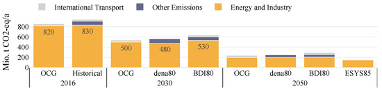
Figure 3.
Annual German GHG emissions. Emissions from agriculture and waste sectors are aggregated under “other emissions”. The ESYS study considers only energy-related emissions. International transport emissions are not part of the national balance.
4.2. Primary Energy Use
A comparison of the computed primary energy consumption for the different studies is shown in Figure 4. For 2016, OCG reproduces the historic total primary energy consumption up to 6% difference. The major remaining difference is the missing use of biomass-based electricity production in the OCG model. This is due to the high costs for this technology, which are also observed in reality and lead to strong subsidies for this sector. The biomass generation could be forced into the model by additional constraints, but we prefer to keep the model more compact.
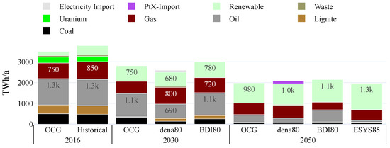
Figure 4.
Annual primary energy use. Renewables include biomass and electricity obtained from wind, photovoltaic (PV), or hydropower plants.
Concerning future developments, the OCG model shows a reduction in primary energy use by 44%, similar to the other studies. This is mostly due to higher efficiency in the electricity generation, transport, and heating sectors, as well as reduced demand for DH. The OCG model values are within the range of the other works. They show a large increase in renewables, a phase-out of coal, and a significant reduction in oil and gas use.
4.3. Electricity Generation
Figure 5 presents results for the electricity generation sector, both the (active) power plant capacities, and the annual generation values. In all studies, a fast expansion of VRE capacities can be observed. The capacities of the OCG model are in the range of the dena80 and BDI80 models. One explanation is that we used the full load hours and costs assumptions of dena80.
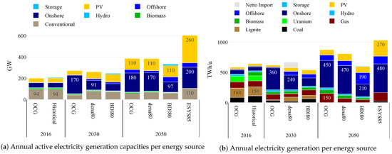
Figure 5.
Electricity generation sector. The term gas includes electricity generation from any type of gas, whether fossil or from biological or synthetic sources.
Concerning dispatchable generation, we observe a gradual shut down of coal-fired power plants across all studies. Note that this occurs in the OCG model without any additional constraints. Shared by all studies is also a significant remaining fleet of gas-fired power plants in the order of the electric peak demand. This is again not explicitly enforced a constraint in the OCG model but follows from satisfying the electricity demand during time slices with low VRE production.
4.4. Electricity Consumption
Figure 6 shows the electricity consumption per application area for all studies, as far as it is made transparent in each study. It gives an important hint of the electrification processes and sector coupling steps taken in each model.
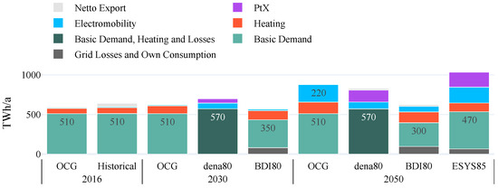
Figure 6.
Annual electricity demand. The basic electricity demand of the OCG model includes losses and self-consumption of power plants (62 TWh/a).
The OCG model’s overall electricity demand increase for 2030 and 2050 is in the range of the other studies for 2030 and 2050. The exception is BDI80, which models a decrease in the basic electricity demand that is assumed to remain constant in OCG. The OCG model provides significant electricity for the electrification of heating and transport in line with the other studies. Unlike dena80 and ESYS85, however, Power-to-X (PtX) does not play a role in the OCG model results nor the BDI80. This technology option is available to the model but is not selected by the optimization algorithm, as the CO2 emission targets can be achieved in other ways, specifically via a higher electrification share in the transport and heating sector.
4.5. Heat Sector
We compare the shares of the different heating technologies in Figure 7. OCG and BDI80 describe the decentral heat sector in terms of the energy supplied by each technology, while the dena80 and ESYS85 refer to the number of heating systems of a particular type. To enable a comparison, we show the relative fractions of energy generation or the number of systems. This is justified since the two values are proportional according to our assumptions above.
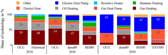
Figure 7.
Technology mix of the decentral heat supply. The shares present both the number of heating systems as well as their relative heat generation.
All models show a significant increase in heat pumps and that they play the dominant role in 2050. Except for dena80, all studies also predict an extension of heating grids. Similar to the other models, the OCG model also shows a remaining share of decentral gas heating in 2050.
4.6. Transport Sector
We compare the different options for future road traffic in Figure 8. As discussed above, the compact OCG model does not distinguish between passenger cars and trucks. The benchmarks studies, however, do make this distinction. We thus compare the OCG results against the car segment of the other studies. As for the heating sector, we show the relative shares of the segment, which allows us to easily unify results given in terms of the number of cars or the energy used for certain car technology.
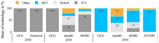
Figure 8.
Technology mix of road traffic. Vehicles powered by hydrogen and gas are categorized as Other The OCG does not consider hybrid vehicles.
In all models, road traffic is significantly electrified. Since OCG does not consider hybrid technologies and does not limit technology shares, the ratios of different technologies are more extreme than in the other studies but comparably close to ESYS85. All studies see major electrification rather in 2050 than already in 2030.
5. Discussion and Conclusions
In this work, we provide an open and compact model for the German energy transition that is highly accessible for new users. The model can represent today’s energy system with high precision, e.g., reproducing the primary energy use with a deviation of less than 6% and the total electricity generation up to 10%. The technology mix for electricity, heat, and transport generation is also well-matched.
For an 80% CO2 reduction target, the model delivers the same key insights as other leading studies [1,2,3]. These are a fast expansion of VREs, a coal phase-out until 2035 while significant gas-fired electricity generation capacities remain in 2050, a rising electricity demand, heat pumps and district heating dominating the heating sector, strong electrification of traffic, but rather after 2030, and uncertain importance of PtX in 2050, at least for the studied −80% reduction targets. These key insights for policy-making are further detailed in [1,2,3]. The compactness of our model justifies the remaining differences to the other studies, which are much more detailed. Their high model complexity allows them to study discuss specific technologies and policy implications in more detail than our approach; however, even with their high detail, they still yield strongly different values for various important indicators. This supports the notion that the large uncertainties about future developments set tight limits on the decision-relevant level of model detail.
The model can easily be adapted to study other reduction targets. Most notably, there has recently been a shift of political targets towards achieving −100% CO2 already in 2045, supported by a first study [43]. The model can also be extended to include additional technologies or changed to accommodate different price or technology assumptions. The reduced number of time steps presented in this work does not allow for detailed storage modeling, the model just considers infinite fuel storage capabilities. Simulations with higher time resolution, or even all time steps of one year, could be computationally feasible by examining single years with fixed capacities. In this case, storage equations as in OSeMOSYS would allow deriving the impact of different storage technologies. Interestingly, however, is that even without storage we are able to recover many important indicators of other studies that include this type of technology.
In future works, we plan to use this model to represent the environment in which multi-modal local energy systems will be inserted. For example, the time-dependent CO2 intensity resulting from simulated future electricity mixes forms a key factor for determining suitable emission reduction measures in local neighborhoods that are interlinked with their environment.
Author Contributions
Conceptualization, J.B., C.R. and F.S.; methodology, J.B., C.R. and F.S.; software, J.B.; validation, J.B.; investigation, J.B.; resources, F.S.; data curation, J.B. and C.R.; writing—original draft preparation, J.B.; writing—review and editing, F.S. and C.R.; visualization, J.B.; supervision, F.S. and C.R.; project administration, F.S.; funding acquisition, F.S. All authors have read and agreed to the published version of the manuscript.
Funding
This research was funded by the German Federal Ministry for Economic Affairs and Energy grant number 03ET1638. We also acknowledge support by the Deutsche Forschungsgemeinschaft (DFG—German Research Foundation) and the Open Access Publishing Fund of Technical University of Darmstadt.
Institutional Review Board Statement
Not applicable.
Informed Consent Statement
Not applicable.
Data Availability Statement
The data presented in this study are available in https://github.com/OCGModel/OCGModel (accessed on 29 November 2021).
Conflicts of Interest
The authors declare no conflict of interest. The funders had no role in the design of the study; in the collection, analyses, or interpretation of data; in the writing of the manuscript, or in the decision to publish the results.
References
- Bründlinger, T.; König, J.E.; Frank, O.; Gründig, D.; Jugel, C.; Kraft, P.; Krieger, O.; Mischinger, S.; Prein, P.; Seidl, H.; et al. Dena-LeitstudieIntegrierte Energiewende—Impulse für die Gestaltung des Energiesystems bis 2050. 2018. Available online: https://www.dena.de/newsroom/publikationsdetailansicht/pub/dena-leitstudie-integrierte-energiewende-ergebnisbericht/ (accessed on 29 November 2021).
- Gerbert, P.; Herhold, P.; Burchardt, J.; Schönberger, S.; Rechenmacher, F.; Kirchner, A.; Kemmler, A.; Wünsch, M. Klimapfade für Deutschland; BCG, The Boston Consulting Group: München, Germany, 2018. [Google Scholar]
- Ausfelder, F.; Drake, F.D.; Erlach, B.; Fischedick, M.; Henning, H.M.; Kost, C.; Münch, W. Sektorkopplung—Untersuchungen und Uberlegungen zur Entwicklung eines Integrierten Energiesystems (Schriftenreihe Energiesysteme der Zukunft); DECHEMA eV: München, Germany, 2017. [Google Scholar]
- Morrison, R. Energy system modeling: Public transparency, scientific reproducibility, and open development. Energy Strategy Rev. 2018, 20, 49–63. [Google Scholar] [CrossRef]
- Pfenninger, S.; DeCarolis, J.; Hirth, L.; Quoilin, S.; Staffell, I. The importance of open data and software: Is energy research lagging behind? Energy Policy 2017, 101, 211–215. [Google Scholar] [CrossRef]
- Pfenninger, S.; Hirth, L.; Schlecht, I.; Schmid, E.; Wiese, F.; Brown, T.; Davis, C.; Gidden, M.; Heinrichs, H.; Heuberger, C.; et al. Opening the black box of energy modelling: Strategies and lessons learned. Energy Strategy Rev. 2018, 19, 63–71. [Google Scholar] [CrossRef]
- Chang, M.; Thellufsen, J.Z.; Zakeri, B.; Pickering, B.; Pfenninger, S.; Lund, H.; Østergaard, P.A. Trends in tools and approaches for modelling the energy transition. Appl. Energy 2021, 290, 116731. [Google Scholar] [CrossRef]
- Herbst, A.; Toro, F.; Reitze, F.; Jochem, E. Introduction to energy systems modelling. Swiss J. Econ. Stat. 2012, 148, 111–135. [Google Scholar] [CrossRef]
- Openmod. Open Energy Modelling Initiative. Available online: https://www.openmod-initiative.org (accessed on 29 November 2021).
- Open Energy Platform. Available online: https://openenergy-platform.org (accessed on 29 November 2021).
- Nikas, A.; Doukas, H.; Papandreou, A. A detailed overview and consistent classification of climate-economy models. In A Detailed Overview and Consistent Classification of Climate-Economy Models, 1st ed.; Doukas, H., Flamos, A., Lieu, J., Eds.; Springer: Cham, Switzerland, 2019; Volume 1, pp. 1–54. [Google Scholar]
- Fishbone, L.G.; Abilock, H. Markal, a linear-programming model for energy systems analysis: Technical description of the bnl version. Int. J. Energy Res. 1981, 5, 353–375. [Google Scholar] [CrossRef]
- Loulou, R.; Goldstein, G.; Noble, K. Documentation for the MARKAL Family of Models. 2004. Available online: https://iea-etsap.org/MrklDoc-I_StdMARKAL.pdf (accessed on 29 November 2021).
- der Voort, E.V. The EFOM 12C energy supply model within the EC modelling system. Omega 1982, 10, 507–523. [Google Scholar] [CrossRef]
- Loulou, R.; Labriet, M. ETSAP-TIAM: The TIMES integrated assessment model Part I: Model structure. Comput. Manag. Sci. 2008, 5, 7–40. [Google Scholar] [CrossRef]
- Howells, M.; Rogner, H.; Strachan, N.; Heaps, C.; Huntington, H.; Kypreos, S.; Hughes, A.; Silveira, S.; DeCarolis, J.; Bazillian, M.; et al. OSeMOSYS: The Open Source Energy Modeling System: An introduction to its ethos, structure and development. Energy Policy 2011, 39, 5850–5870. [Google Scholar] [CrossRef]
- Pfenninger, S.; Pickering, B. Calliope: A multi-scale energy systems modelling framework. J. Open Source Softw. 2018, 3, 825. [Google Scholar] [CrossRef]
- Hilpert, S.; Kaldemeyer, C.; Krien, U.; Günther, S.; Wingenbach, C.; Plessmann, G. The Open Energy Modelling Framework (oemof)—A new approach to facilitate open science in energy system modelling. Energy Strategy Rev. 2018, 22, 16–25. [Google Scholar] [CrossRef]
- PyPSA Model of the South African Energy System. Available online: https://github.com/PyPSA/pypsa-za (accessed on 29 November 2021).
- Calliope-Project. Model of the UK Power System Built with Calliope. Available online: https://github.com/calliope-project/uk-calliope (accessed on 29 November 2021).
- Temoa Project. Open Energy Outlook for the United States. Available online: https://github.com/TemoaProject/oeo (accessed on 29 November 2021).
- ENTSO-E. Transparency Platform. 2020. Available online: https://transparency.entsoe.eu (accessed on 25 November 2020).
- Sakellaris, K.; Canton, J.; Zafeiratou, E.; Fournié, L. METIS—An energy modelling tool to support transparent policy making. Energy Strategy Rev. 2018, 22, 127–135. [Google Scholar] [CrossRef]
- Hülsmann, J.; Steinke, F. Explaining Complex Energy Systems: A Challenge. In Proceedings of the 34th Conference on Neural Information Processing Systems (NeurIPS 2020), Virtual Conference, 6–12 December 2020. [Google Scholar]
- Schaber, K.; Steinke, F.; Hamacher, T. Transmission grid extensions for the integration of variable renewable energies in Europe: Who benefits where? Energy Policy 2012, 43, 123–135. [Google Scholar] [CrossRef]
- Fleiter, T.; Elsland, R.; Rehfeldt, M. Heat Roadmap Europe: A low-carbon heating and cooling strategy. Resour. Results 2017, D3.1, 35–48. [Google Scholar]
- Wilms, S.; Lerm, V.; fer Stradowsky, S.S.; Sanden, J.; Jahnke, P.; Taubert, G. Heutige Einsatzgebiete für Power Fuels—Factsheets zur Anwendung von Klimafreundlich Erzeugten Synthetischen Energieträgern; Technical Report; BBHC and Dena and IKEM: Berlin, Germany, 2018. [Google Scholar]
- Energiedaten: Gesamtausgabe. 2021. Available online: https://www.bmwi.de/Redaktion/DE/Artikel/Energie/energiedaten-gesamtausgabe.html (accessed on 4 April 2021).
- Drosihn, D.; Icha, P.; Kuhs, G.; Sandau, F.; Pabst, J.; Hain, B.; Nowakowski, M.; Pfeiffer, D.; Juhrich, K.; Bünger, B.; et al. Daten und Fakten zu Braun- und Steinkohlen; Umweltbundesamt: Dessau, Germany, 2017. [Google Scholar]
- Eltrop, L.; Hartmann, H.; Heinrich, P. Leitfaden Feste Biobrennstoffe. FNR. Fachagentur Nachwachsende Rohst. Gülzow 2014, 4, 146–163. [Google Scholar]
- Technology Data for Industrial Process Heat; Resreport; Danish Energy Agency: Copenhagen, Denmark, 2016.
- Technology Data for Individual Heating Plants; Technical Report; Danish Energy Agency: Copenhagen, Denmark, 2016.
- KBA. Der Fahrzeugbestand im überblick am 1. Januar 2016 Gegenüber 1. Januar 2015. 2016. Available online: https://www.kba.de/DE/Statistik/Fahrzeuge/Bestand/Jahrebilanz_Bestand/2016/2016_b_ueberblick_pdf (accessed on 10 April 2021).
- Icha, P.; Kuhs, G. Entwicklung der Spezifischen Kohlendioxid-Emissionen des Deutschen Strommix in den Jahren 1990–2017; Resreport ISSN 1862-4359; Umweltbundesamt: Dessau-Roßlau, Germany, 2018. [Google Scholar]
- Sauer, D.U.; Görner, K.; Elsen, R.; Wolf, K.-J.; Gasteiger, G.; Katzenberger, H.; Kakaras, E.; Kather, A.; Lindenberger, D.; Oechsner, M.; et al. Konventionelle Kraftwerke—Technologiesteckbrief zur Analyse “Flexibilitätskonzepte für die Stromversorgung 2050”; Schriftenreihe Energiesysteme der Zukunft: Essen, Germany; Aachen, Germany, 2016. [Google Scholar] [CrossRef]
- Palou-Rivera, I.; Wang, M.Q. Updated Estimation of Energy Efficiencies of U.S. Petroleum Refineries; Technical Report; Argonne National Lab. (ANL): Argonne, IL, USA, 2010. [CrossRef]
- Howey, D.; Martinez-Botas, R.; Cussons, B.; Lytton, L. Comparative measurements of the energy consumption of 51 electric, hybrid and internal combustion engine vehicles. Transp. Res. Part D Transp. Environ. 2011, 16, 459–464. [Google Scholar] [CrossRef]
- Report on Conversion Efficiency of Biomass; Research Report; BASIS-Biomass Availability and Sustainability Information System: Bonn, Germany, 2015.
- Steinbach, J.; Staniaszek, D. Discount Rates in Energy System Analysis; Fraunhofer ISI and Building Performance Institute Europe (BPIE): Brussels, Belgium, 2015. [Google Scholar]
- Bundesnetzagentur. Kraftwerksliste. 2019. Available online: https://www.bundesnetzagentur.de/DE/Sachgebiete/ElektrizitaetundGas/Unternehmen_Institutionen/Versorgungssicherheit/Erzeugungskapazitaeten/Kraftwerksliste/start.html (accessed on 12 June 2019).
- Wie Heizt Deutschland? Technical Report; BDEW: Berlin, Germany, 2015.
- Abwicklung von Standardlastprofilen Gas; Technical Report; BDEW, VKU and GEODE: Berlin, Germany, 2018.
- Klimaneutrales Deutschland; Study Commissioned by Studie im Auftrag von Agora Energiewende, Agora Verkehrswende und Stiftung Klimaneutralität, Technical Report; Prognos: Basel, Switzerland; Öko-Institut: Breisgau, Germany; Wuppertal-Institut: Wuppertal, Germany, 2020.
Publisher’s Note: MDPI stays neutral with regard to jurisdictional claims in published maps and institutional affiliations. |
© 2021 by the authors. Licensee MDPI, Basel, Switzerland. This article is an open access article distributed under the terms and conditions of the Creative Commons Attribution (CC BY) license (https://creativecommons.org/licenses/by/4.0/).