Article

Design and Implementation of Periodic Control for a Matrix Converter-Based Interior Permanent Magnet Synchronous Motor Drive System

Department of Electrical Engineering, National Taiwan University of Science and Technology, Taipei 106, Taiwan
*
Author to whom correspondence should be addressed.
Energies 2021, 14(23), 8073; https://doi.org/10.3390/en14238073
Submission received: 28 October 2021 / Revised: 23 November 2021 / Accepted: 30 November 2021 / Published: 2 December 2021
(This article belongs to the Special Issue Design and Control of Electrical Motor Drives II)

Abstract

:
The matrix converter-based IPMSM drive has 360 Hz virtual DC-bus voltage variations which produce severe stator harmonic currents. To solve this problem, a speed-loop classical periodic controller and two current-loop periodic controllers, including a classical periodic controller and a selective harmonic controller, are proposed in this paper. By using the proposed methods, the harmonic currents are obviously reduced and the speed responses of the IPMSM are clearly improved. A detailed analysis is discussed. A digital signal processor, type SH7237, manufactured by Renesas Electronics Corporation is used for the control algorithms. Experimental results show that those proposed periodic controllers reduce up to nearly 32% of the total harmonic distortion at the stator currents, and also apparently improve the transient, tracking, and repetitive load disturbance speed responses.

1. Introduction

Matrix converter (MC) based permanent magnet synchronous motor (PMSM) drives have many advantages, including bi-directional power flows, single-stage power conversion, a unity input power factor, low input harmonic currents, high efficiency, small size, and no need for a large electrolytic capacitor. Several researchers have focused on the MC-based PMSM drives in various aspects. For example, many researchers have investigated sensorless techniques for MC-based PMSM drives to adjust their speeds from standstill to high-speed operating ranges [1,2]. Several researchers have proposed fault tolerant control for MC-based PMSM drives even though open-switch faulty conditions occurred [3,4]. Furthermore, other researchers studied the improvements of the current commutation methods of the MC-based PMSM drives to enhance their output current waveforms [5,6].
MC-based PMSM drives, however, have some disadvantages as well. For example, the virtual DC-link voltage has a frequency which is six times higher than the input voltage frequency. In addition, MC-based PMSM drives require three-step or four-step phase current commutation algorithms. Both the voltage variations and phase current commutations produce obvious output current harmonics, torque pulsations, and speed ripples. To improve MC-based PMSM drives, several different methods have been investigated. For example, Xiao et al. proposed a sensorless MC-based interior permanent magnet synchronous motor (IPMSM) drive. By using the two closed-loop PI control algorithms of the torque and the flux separately, high dynamic responses and good steady-state characteristics over a wide operating range of IPMSM drives were achieved [7]. Gong et al. used quasi-proportional resonant controllers for an indirect MC-based PMSM drive. By using resonant controllers, the control complexity was simplified and the execution time of the digital signal processor (DSP) was shortened [8]. Wisniewski et al. studied a Petri net-based algorithm to control a direct MC-based PMSM drive. An FPGA was used to provide concurrent computations [9]. Kumar et al. used an adaptive fuzzy logic controller for an energy-efficient optimization-based control algorithm of an MC-fed wind energy conversion system [10]. Xia implemented an internal model principle (IMP) control for an MC-based PMSM drive system to reduce the influences of the input voltage disturbances [11]. Yao proposed distributed control for a multilevel MC which was applied in medium-voltage and high-power applications [12]. Monteiro et al. proposed a sliding-mode controller for a MC-based PMSM drive that was operated with unified power flow controllers [13]. Formentini et al. investigated a predictive controller for an MC-based PMSM drive. That paper used the same control algorithm for both the current-loop and speed-loop of the PMSM [14].
Since 2020, an increasing number of researchers have focused on modulation methods and predictive controller design for matrix converters. For example, Shigeuchi et al. proposed a modulation method for matrix converters to achieve zero-voltage-switching and sinusoidal line currents under bidirectional operation with PQ control [15]. Lei et al. investigated a simple modulation scheme with zero common-mode voltages for matrix converter-based PMSM drive systems [16]. Szczepankowski et al. proposed using analytic signals and smooth interpolation in pulse-width modulation for matrix converters [17]. Li et al. implemented an overmodulation strategy for matrix converters under unbalanced input voltages [18]. Deng et al. used a multidimensional switching table for the minimizing common-mode voltages of matrix converter-based PMSM drive systems [19]. In addition, Fang et al. proposed coordination control of a modulation index and a phase-shift angle for matrix converters [20]. Urrutia implemented circulating current control for multilevel matrix converter-based predictive control [21]. Mir et al. designed model predictive control for speed sensorless matrix converter-based drive systems [22]. Fang studied finite control-set model-predictive control for matrix converters with virtual space vectors [23]. The previously published control methods for matrix converter based AC drives are shown in Table 1. To the best of our knowledge, no previously published paper has investigated the application of using periodic control for matrix converter-based AC motor drive systems.
To fill this research gap, in this paper, a speed-loop periodic controller and two current-loop periodic controllers are investigated. The periodic current control can effectively reduce the current harmonics at the stator, and the periodic speed control can obviously improve the transient responses, load disturbance responses, and tracking responses of the motor speed. In addition, a DSP and an FPGA use parallel computations to serve as the control center of the IPMSM drive. Measured results show the proposed periodic control IPMSM drive can be fed by a silicon carbide MC, which is operated at a 50 kHz switching frequency, which is nearly five times faster than traditional IGBT-based PMSM drives. To the authors’ best knowledge, the ideas mentioned here are completely original and are also discussed for the first-time in this paper.

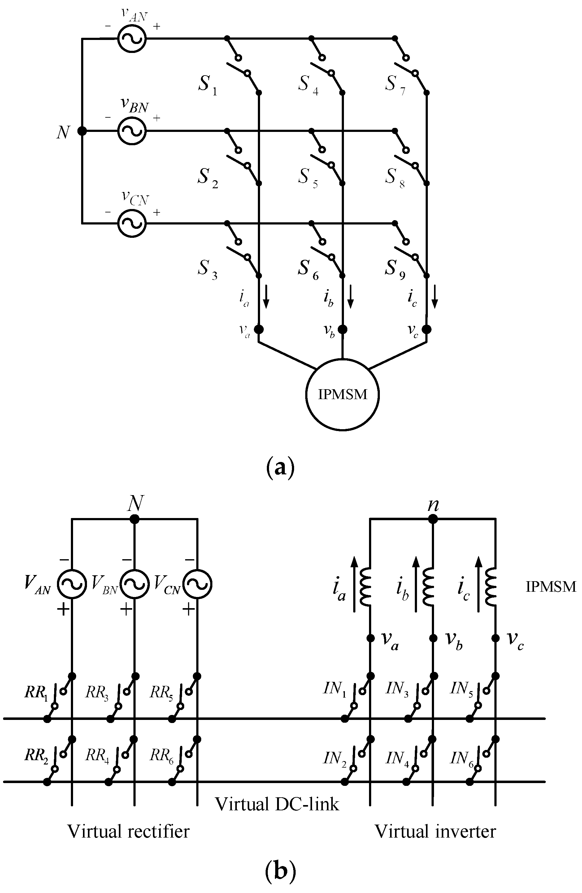
2. Matrix-Converter Based IPMSM Drives

An MC-based IPMSM drive is investigated in this paper. In this section, the main circuit of the matrix converter is discussed first, and then its equivalent circuit is introduced later. After that, the mathematical model of the IPMSM is discussed. The details are shown as follows:

2.1. Matrix Converter

Matrix converters (MC) were first proposed in the late 1970s, and they have gradually become more and more popular due to their having regeneration ability, sinusoidal input currents, a unity input power factor, small size, bi-directional power flows, and no need for electrolytic capacitors [24].
The main circuit of an MC is shown in Figure 1a, which includes three-phase input voltage sources and three-phase output current sinks. The relationship between the three-phase output voltages and three-phase input voltages are as follows:
[ v a v b v c ] = [ S 1 S 2 S 3 S 4 S 5 S 6 S 7 S 8 S 9 ] [ V A N V B N V C N ]
where v a , v b , and v c are the three-phase output voltages, V A N , V B N , and V C N are the three-phase input voltages, and S 1 , S 2 , S 3 , S 4 , S 5 , S 6 , S 7 , S 8 , and S 9 are the AC switches.
Figure 1b shows the equivalent circuit of the MC, which includes a virtual rectifier and a virtual inverter. The virtual rectifier converts the three-phase AC input voltages into a virtual DC-link voltage. In addition, the virtual inverter converts the virtual DC-link voltage, V d c , to three-phase variable frequencies and three variable output voltages, v a , v b , and v c . Finally, the voltages v a , v b , and v c are used to adjust the torque and speed of the IPMSM. The relationship between the virtual DC-link voltage and the three-phase input voltages is shown as follows:
[ 0.5 V d c 0.5 V d c ] = [ R R 1 R R 3 R R 5 R R 2 R R 4 R R 6 ] [ V A N V B N V C N ]
The relationship between the three-phase output voltages and the virtual DC-link voltage is:
[ v a v b v c ] = [ I N 1 I N 2 I N 3 I N 4 I N 5 I N 6 ] [ 0.5 V d c 0.5 V d c ]
Substituting Equation (2) into Equation (3), one can obtain:
[ v a v b v c ] = [ I N 1 I N 2 I N 3 I N 4 I N 5 I N 6 ] [ R R 1 R R 3 R R 5 R R 2 R R 4 R R 6 ] [ V A N V B N V C N ]
Finally, from Equations (1) and (4), one can obtain the relationship between the output voltages and the input voltages of the matrix converter as follows:
[ S 1 S 2 S 3 S 4 S 5 S 6 S 7 S 8 S 9 ] = [ I N 1 I N 2 I N 3 I N 4 I N 5 I N 6 ] [ R R 1 R R 3 R R 5 R R 2 R R 4 R R 6 ]
Generally speaking, the output currents of the MC cannot be abruptly interrupted because the inductance of the motor may generate huge spikes that then destroy the power devices. In addition, the operation of the power switches in an output line cannot have more than one power switch turning on because this will cause a short-circuit of the input voltage sources.
Figure 1c shows the voltage waveform across the virtual DC-link when a three-phase 60-Hz 220-V AC input voltage source is used. As we can observe, the virtual DC-link voltage fluctuated from 270 V to 311 V. The main reason is that the input voltage V A B , V A C , V B C , V B A , V C A , and V C B sequentially appears in the virtual DC-link. In addition, no electrolytic filtering capacitor is indeed virtual and not real. For a conventional AC/DC/AC conversion, a three-phase rectifier is used to convert the three-phase AC voltage into DC voltage. Then, a large filtering electrolytic capacitor is used to eliminate the 360 Hz voltage ripples. After that, a space-vector pulse-width modulation method is used to generate three-phase output voltages. For matrix converter-based AC motor drive systems, the 360 Hz voltage ripples cause serious 5th and 7th harmonic currents. To solve this problem of harmonic currents of matrix converter-based PMSM drive systems, in this paper, a selective harmonic periodic controller is proposed to reduce the 5th and 7th harmonic currents. In addition, a conventional periodic controller is proposed to reduce the speed drop when a repetitive external load is added. These are the main research goals of this paper.

2.2. Mathematical Model of an IPMSM

The IPMSM discussed in this paper has a high torque/ampere ratio, robust structure, and high power density, and it easily executes field weakening control and sensorless control. Generally speaking, the IPMSM has a smaller inductance at the d-axis than at the q-axis. In the d-q synchronous axis, the differential equations of the d-q axis currents are described as follows:
d i d s d t = 1 L d s ( v d s R s i d s + P 2 ω r m L q s i q s )
and
d i q s d t = 1 L q s ( v q s R s i q s ) P 2 ω r m ( λ m + L d s i d s )
where i d s and i q s are the d-q axis currents, d d t is the differential operator, L d s and L q s are the d-q axis inductances, v d s and v q s are the d-q axis voltages, R s is the stator resistance, P is the pole number, ω r m is the mechanical speed, and λ m is the flux linkage.
The electromagnetic torque of the IPMSM is shown as follows:
T e = 3 2 P 2 ( λ m i q s + ( L d s L q s ) i d s i q s )
The rotor mechanical speed is:
d d t ω r m = 1 J m ( T e T L B m ω r m )
The rotor electrical speed is:
ω e = P 2 ω r m
Finally, the rotor electrical position is:
θ e = P 2 θ r m

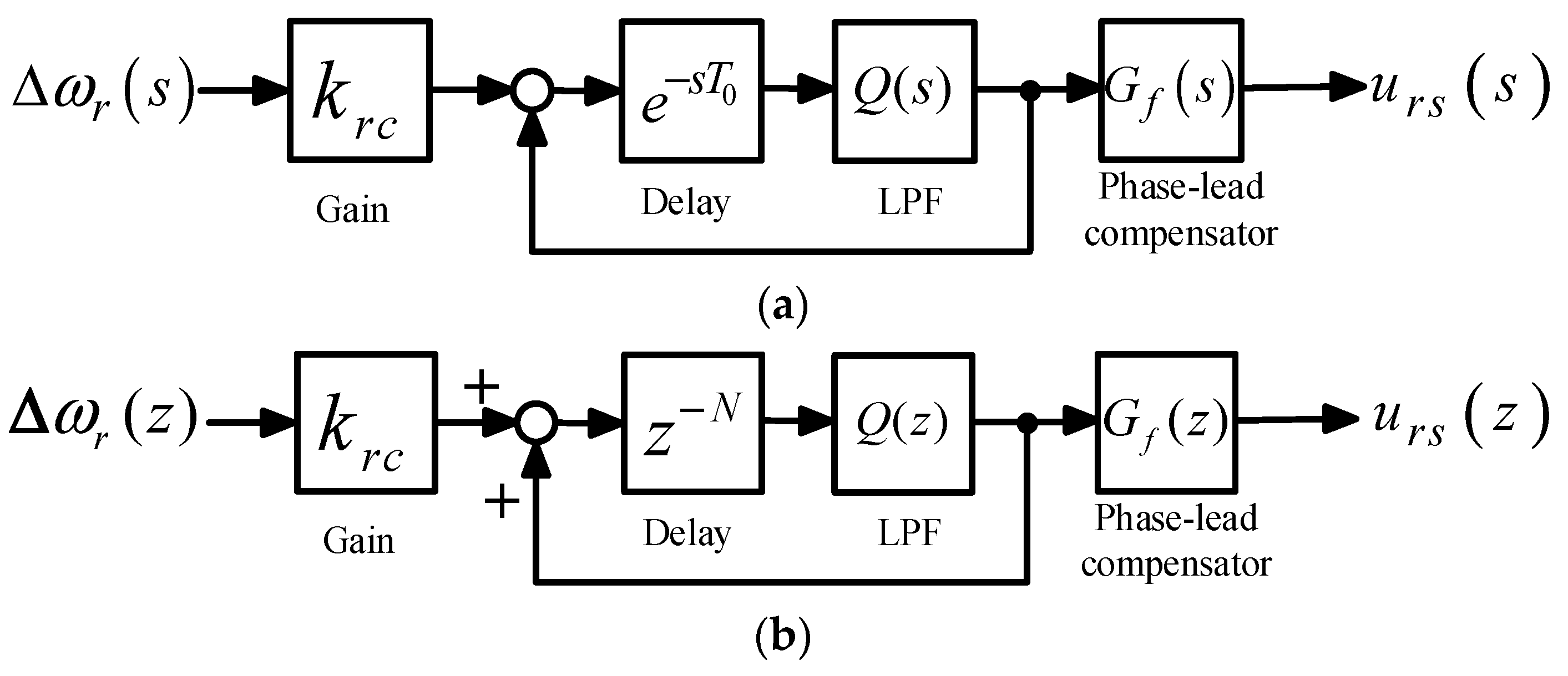
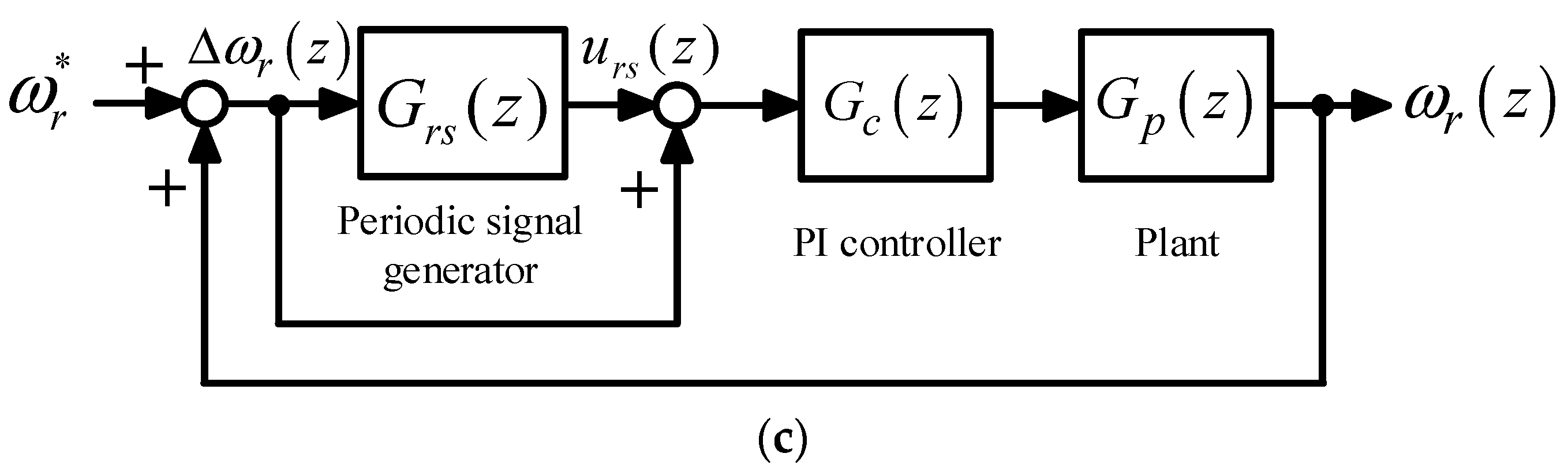
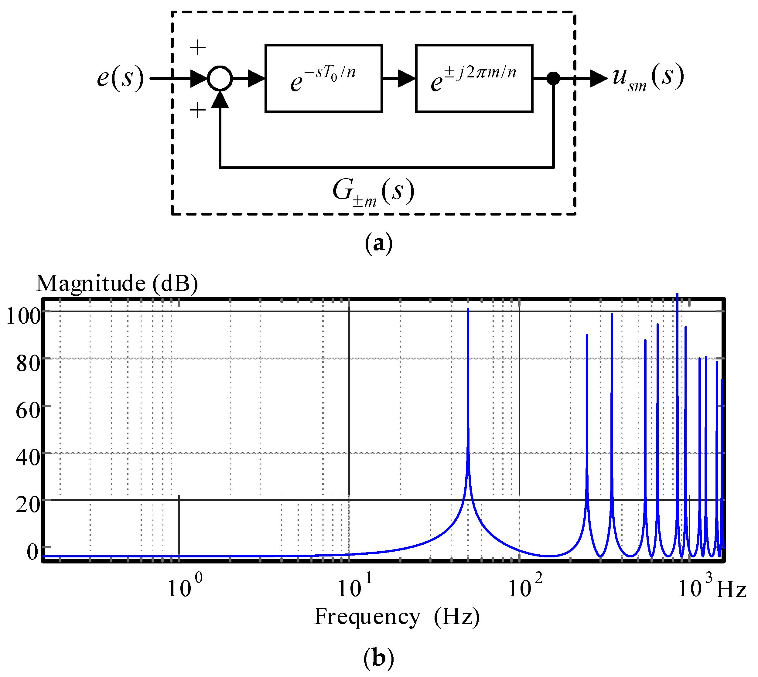
3. Speed-Loop Periodic Controller

The speed-loop controller of the MC-based IPMSM drive uses a classical periodic controller (CPC) to improve its performance. The details are as follows:

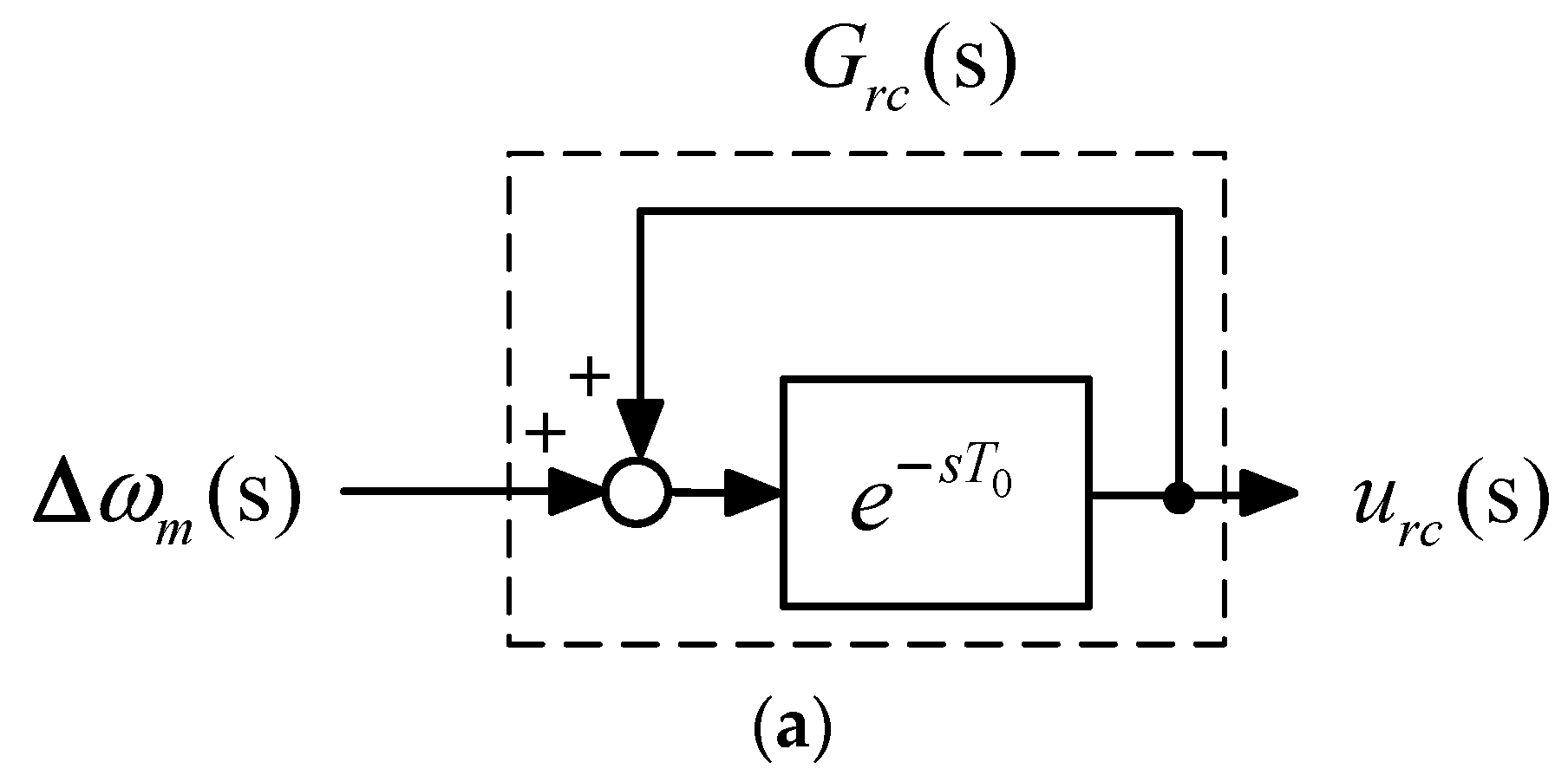
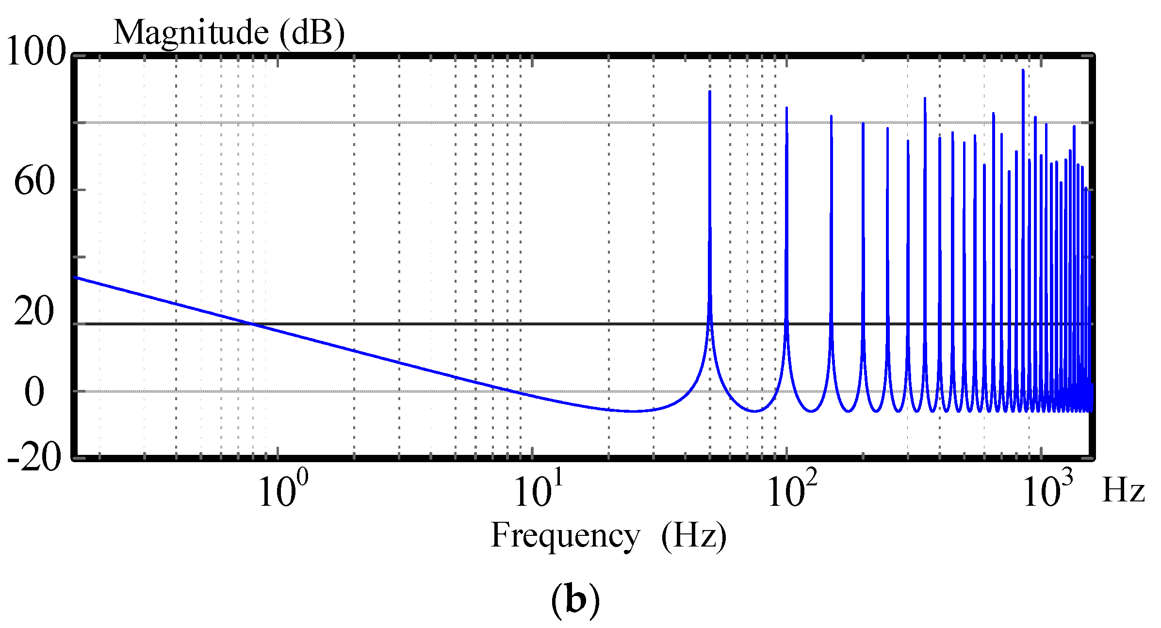
3.1. Classical Periodic Controller

In this section, the basic principle is discussed first, and then a detailed stability-analysis is given, and is followed by determination of the control parameters.

3.1.1. Basic Principle

The concept of a CPC was used in long-wall coal cutting and metal rolling in England in the early 1970s [25]. The design of a CPC is based on the internal model principle (IMP), which states that the control input of a perfect asymptotic rejection and tracking system can be obtained by inserting a signal generator into a stable feedback control system [26]. The concept of this internal model is expressed as follows:
Any good regulator needs to create a model of its dynamic in the closed-loop system. For example, a method used for removing the sinusoidal periodic disturbances, such as vibrations and current harmonics, needs to have a mathematical model of the periodic disturbances as multiple sinusoids. These sinusoids can be modeled as a disturbance-generating polynomial as follows:
γ d ( s ) = i = 1 m ( s 2 + ω i 2 )
where γ d ( s ) is the polynomial of the multi sinusoids, and ω i is their different frequencies. Generally speaking, a closed-loop system includes a transfer function between the output and the reference-input and also a transfer function between the output and the external disturbance. Each transfer function consists of a nominator polynomial divided by a denominator polynomial. When the denominator polynomial of the output to the reference-input and the denominator of the output to the disturbance-input share some common roots, then these common roots are included in the denominator of the controller to satisfy the IMP. In other words, the internal model principle states that the output of a closed-loop system can track the reference commands and also can reject the external disturbances well if a suitable high frequency generator is inserted into the closed-loop system [10,11]. The details are shown as follows:
In order to realize the γ d ( s ) shown in Equation (12), a corresponding transfer function of an IMP-based resonant controller is shown as:
G h ( s ) = L   ( ( K h cos ( ω h t + φ h ) ) = K h s cos φ h ω h sin φ h s 2 + ω h 2
where L is the Laplace transformation, K h is the control gain that is used to tune the error converge rate, φ h is the phase-lead angle for the delay compensation, s is the symbol in the s-domain that is generated from the Laplace transformation, and ω h is the resonant frequency. To simplify the problem, one can assume that φ h is zero. Then, the corresponding transfer function of an IMP-based resonant controller is shown as:
G h ( s ) = K h s s 2 + ω h 2
and
ω h = h ω 0
where h is the order of harmonics and ω 0 is the resonant frequency. In the real world, the transfer function G h ( s ) shown in Equation (15) is very complicated and difficult to implement because it is a second-order band-pass controller. To solve this problem, a periodic signal generator is used to replace the band-pass controller. The details are as follows:
Figure 2a shows the basic concept of the periodic generator. The generator is synthesized by using a delay T 0 device and unit positive feedback in a continuous-time domain. According to Figure 2a, the transfer function of the periodic signal generator is derived as:
G r c ( s ) = u r c ( s ) Δ ω m ( s ) = e s T 0 1 e s T 0
where T 0 = 2 π ω 0 = 1 f 0 is the period of the high-frequency signal and ω 0 is the angular frequency. The transfer function of the periodic signal generator G r c ( s ) , which is shown in Equation (16), is expanded as follows [20]:
G r c ( s ) = 1 2 + 1 s T 0 + 1 T 0 n = 1 2 s s 2 + ( n ω 0 ) 2
From Equation (17), the periodic signal generator includes three parallel combinations: an impulse signal gain 1 2 , a step input transfer function 1 s T 0 , and a transfer function of high-frequency harmonics 2 s s 2 + ( n ω 0 ) 2 . Moreover, the periodic signal generator has different poles at s = ± j n ω 0 . The periodic signal generator, therefore, produces infinite gains at different n ω 0 harmonic frequencies, which are shown in Figure 2b. As a result, the CPC can produce near zero-tracking errors at each n ω 0 frequency.
In the real world, a low-pass filter Q(s) is required to reduce harmonics, and a phase-lead compensator G f ( s ) is required to improve the phase margin of the closed speed-loop. From Figure 3a, after transforming the s-domain into the z-domain, one can obtain Figure 3b. The details of the z-domain periodic signal generator, shown in Figure 3b, is discussed as follows:
The transfer function of the discrete-domain periodic signal generator is expressed as:
G r s ( z ) = k r c Q ( z ) z N 1 Q ( z ) z N G f ( z )
where k r c is a constant gain, Q ( z ) is a low-pass filter (LPF), G f ( z ) is a phase-lead compensator, and N is the number of delay steps.
In the discrete time domain, the z N , is added as shown in Figure 3b. N can be expressed as:
N = T 0 T s
where T 0 is the delayed period, and T s is the sampling interval of the speed-loop control system. The delayed period T 0 is divided by T s to determine the delayed N steps, which are shown in Equation (19). To obtain a smooth transient response, a PI controller G c ( z ) is inserted into the forward loop, which is shown in Figure 3c. In Figure 3c, G r s ( z ) is the periodic signal generator that is used to reject periodic disturbances, G c ( z ) is the speed-loop PI controller to obtain smooth transient responses, and G p ( z ) is the transfer function of the uncontrolled plant. Figure 3c shows the closed-loop discrete-time CPC speed-control system.
The fundamental concept of this CPC speed control system is explained as follows. In Figure 3c, in normal operation, the u r s is very small. As a result, the Δ ω r uses a PI controller, G C ( z ) , to generate an input control signal to the plant. In this situation, the closed-loop speed control system is similar to a normal closed-loop PI control system. For every N times of the sampling interval, the periodic signal generator creates a large output of u r s to add to Δ ω r , and then the summation is sent to the PI controller, G C ( z ) , to control the plant, G p ( z ) . In this situation, the closed-loop speed control system becomes a high-gain controller system to reduce the speed error, Δ ω r . As a result, the real speeds can track speed commands well. By using this method, the speed error can be effectively reduced, especially when a repetitive external load is added.
The speed-loop CPC has the following parameters: a gain k r c and a phase-lead compensation G f ( z ) , which are determined by using the following stability analysis.

3.1.2. Stability Analysis and Control Parameter Determination

The closed-loop speed control IPMSM system is shown in Figure 3c. From Figure 3c, one can obtain the following equation [27]:
Δ ω r ( z ) = 1 Q ( z ) z N 1 [ ( 1 K r c G f ( z ) H ( z ) ) Q ( z ) ] z N Δ ω r 0 ( z )
and
H ( z ) = G c ( z ) G p ( z ) 1 + G c ( z ) G p ( z )
where Δ ω r 0 ( z ) is the initial value of the speed error, Δ ω r ( z ) is the k-th sampling-time speed error, and H(z) is the closed-loop transfer function obtained by using the PI controller, which is expressed as G c ( z ) , to achieve unity feedback. From Equation (20), one can derive that Δ ω r ( z ) is:
Δ ω r ( z ) = A ( z ) · z N Δ ω r ( z ) + [ 1 Q ( z ) z N ] Δ ω r 0 ( z )
and
A ( z ) = ( 1 k r c G f ( z ) H ( z ) ) Q ( z )
The stability criterion of (23) is | A ( z ) | < 1 . The closed-loop transfer function without considering the external load is expressed as:
H ( e j ω ) = | H ( e j ω ) | e j θ H ( ω )
Submitting Equation (24) into the stability criterion | A ( z ) | < 1 , and also assuming ( 2 k π π 2 ) < ( θ f H ) < ( 2 k π + π 2 ) , one can obtain the following inequality:
0 < k r c < 2 cos ( θ f H ) | H ( e j ω ) |
and
θ f H = θ H + p ω
where θ H is the phase angle of H(z), ω is the frequency, p is the order of the phase-lead compensation, θ f H is the total angle of θ H and p ω , and H ( z ) is the transfer function of the closed-loop PMSM speed control system. Thus, the controller parameters k r c an p are determined, and the phase-lead compensation G f ( z ) can be commonly expressed as follows:
G f ( z ) = z p
The parameter selections of the closed-loop speed-control drive system are discussed here. Figure 4a shows the relationship between the boundary of the phase angle and operating frequency. The different phase lead steps p provide different ( θ H + p ω ) angles. By selecting p = 1 and by using frequencies shown in Figure 4a, one can obtain the widest operating frequency in the allowed phase angles between 90° and −90°. As a result, in this paper, the phase lead compensator G f ( z ) is selected as z 1 . Next, the gain k r c is chosen according to stability analysis, which is shown in Equation (25). From Equation (25), the gain k r c needs to satisfy the inequality equation. Figure 4b demonstrates the relationship between the maximum boundary ( 2 cos ( θ H + p ω ) / | H ( e j ω ) | ) and the operation frequency. By choosing the y-axis minimum point of the curve and by using p = 1 in Figure 4a, one can obtain the value of the gain as 1.4. Then from Equation (25), the gain   k r c   should be between 1.4 and 0. To simplify the computation for the CPC speed control-loop, k r c = 1 was selected in this paper.
The low-pass filter Q ( z ) is chosen here because it is commonly used in digital filter applications. The transfer function of an FIR LPF Q ( z ) can be expressed as:
Q ( z ) = a 0 + a 1 z 1 + a 2 z 2
The components of the periodic controller are shown in Figure 5a. The speed error Δ ω e ( z ) is multiplied by the control gain k r c and then added to the z - p u r s ( z ) to generate e s ( z ) . A delay and a low-pass filter, Q(z), is used to reduce the high-frequency noise. The parameters include a 0 = 0.275 , a 1 = 0.45 , and a 2 = 0.275 , which were obtained from a computer simulation with a bandwidth of 1 kHz and a cut off frequency of 5 kHz.
In order to easily explain the periodic control more clearly, Figure 5a–d is provided. Figure 5a shows the block diagram of the closed-loop periodic control IPMSM drive system, which includes a periodic signal generator G r c ( z ) , a PI speed-loop controller G c ( z ) , and an uncontrolled plant G p ( z ) . Figure 5b shows the typical speed error Δ ω r ( z ) response of the step-input speed command. From this figure, we can see that the speed error Δ ω r ( z ) converges to zero quickly. The dynamic response of the Δ ω r ( z ) depends on the uncontrolled plant G p ( z ) and the PI controller. Figure 5c shows the response of the periodic input u r c ( z ) , which increases from a small value and reaches a steady-state condition in order to remove the repetitive external load. Figure 5d shows the total control input, which is the summation of the Δ ω r ( z ) and u r c ( z ) .
Compared to traditional speed-loop PI controllers, this proposed speed periodic controller provide an additional control input to remove the repetitive external load. In addition, the digital periodic generator shown in Figure 5a is very simple and is easily implemented by using a DSP.

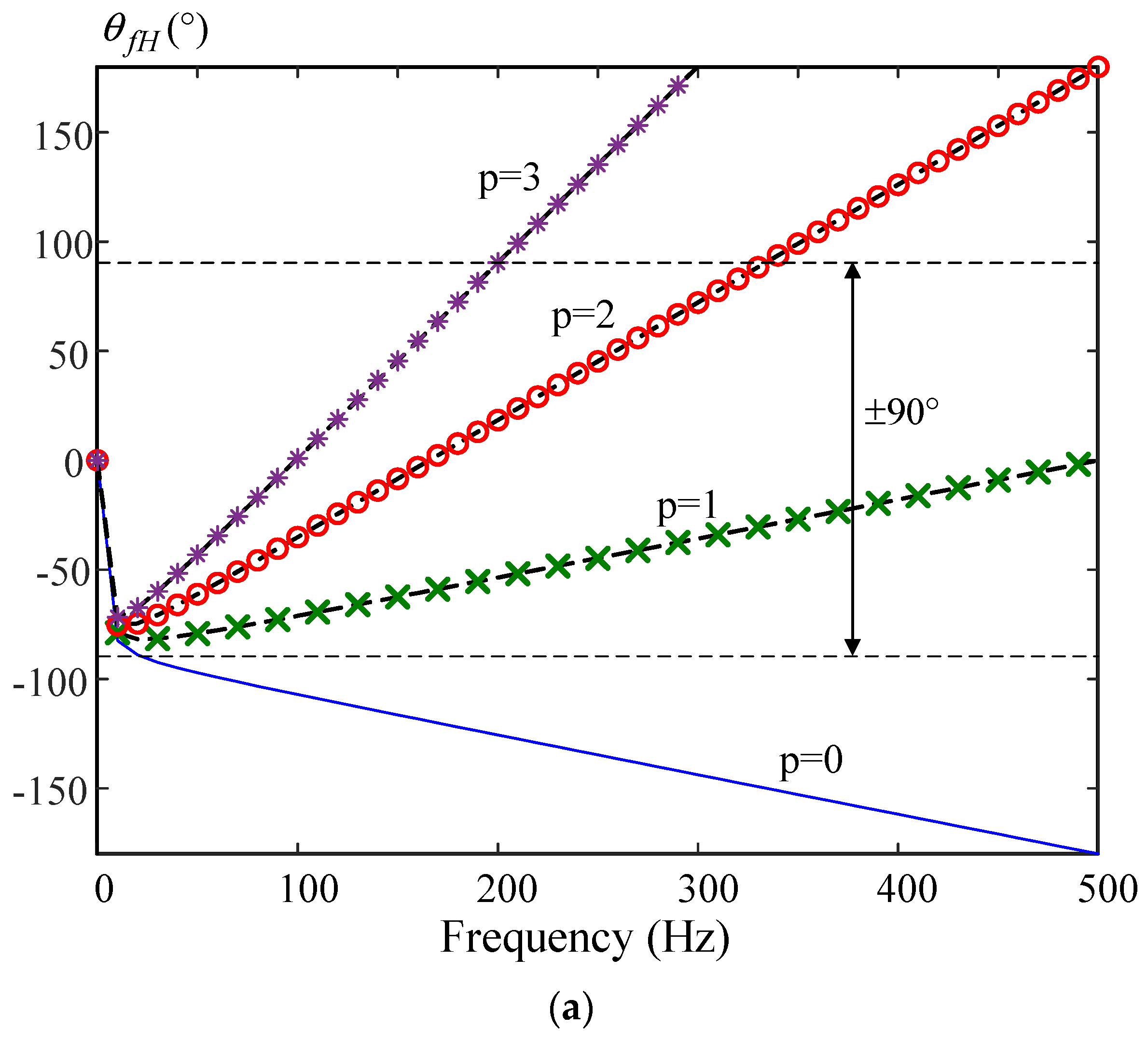
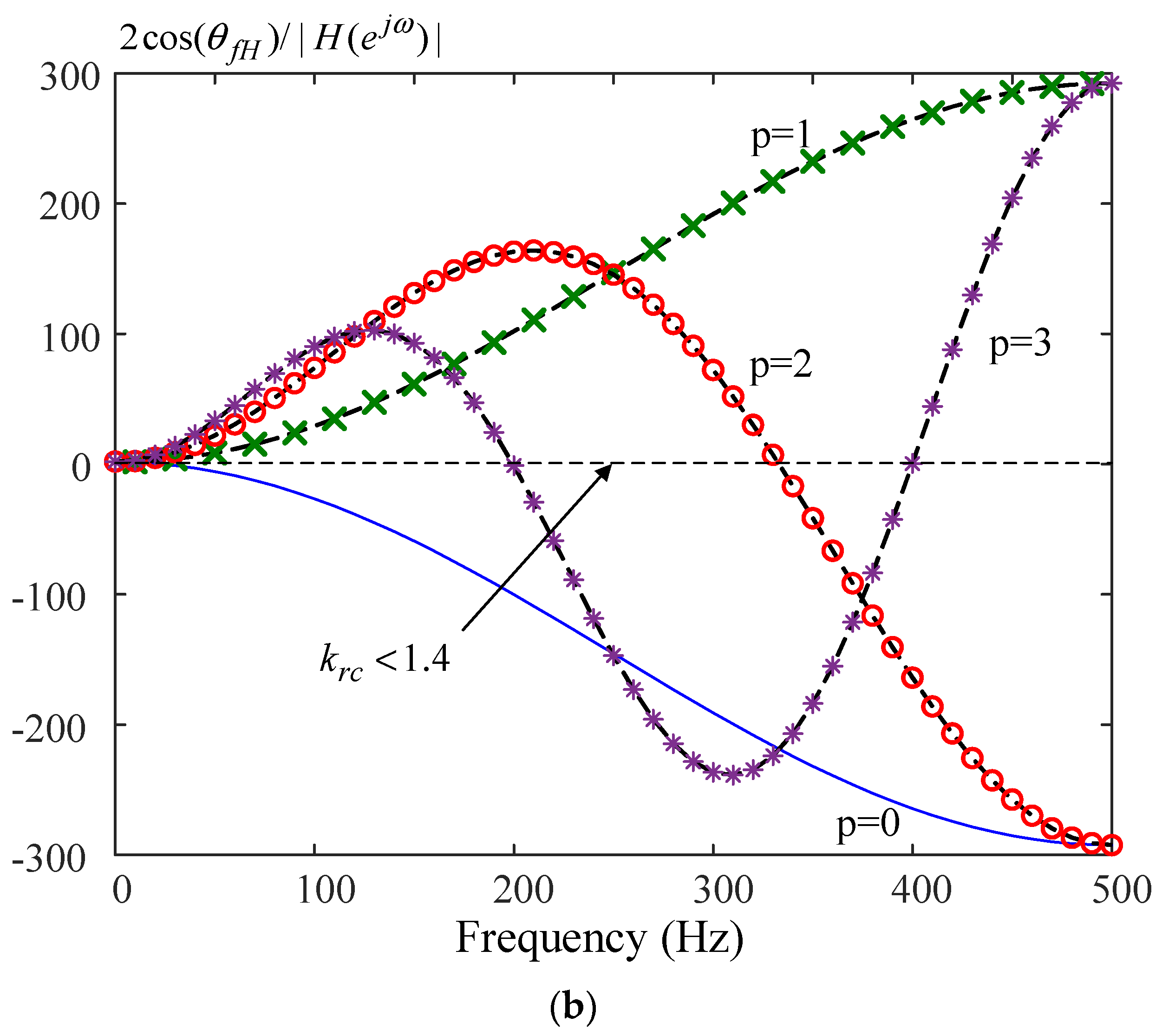
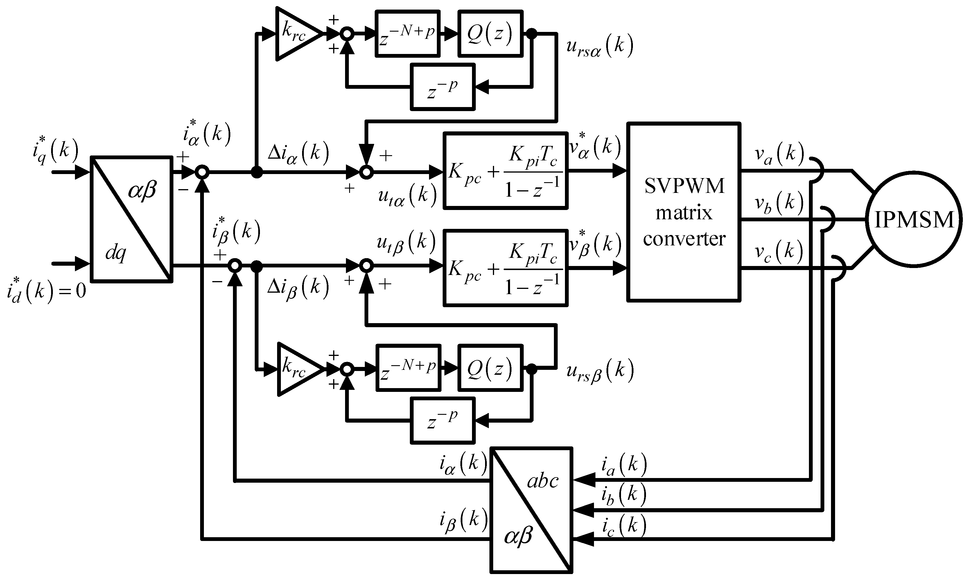
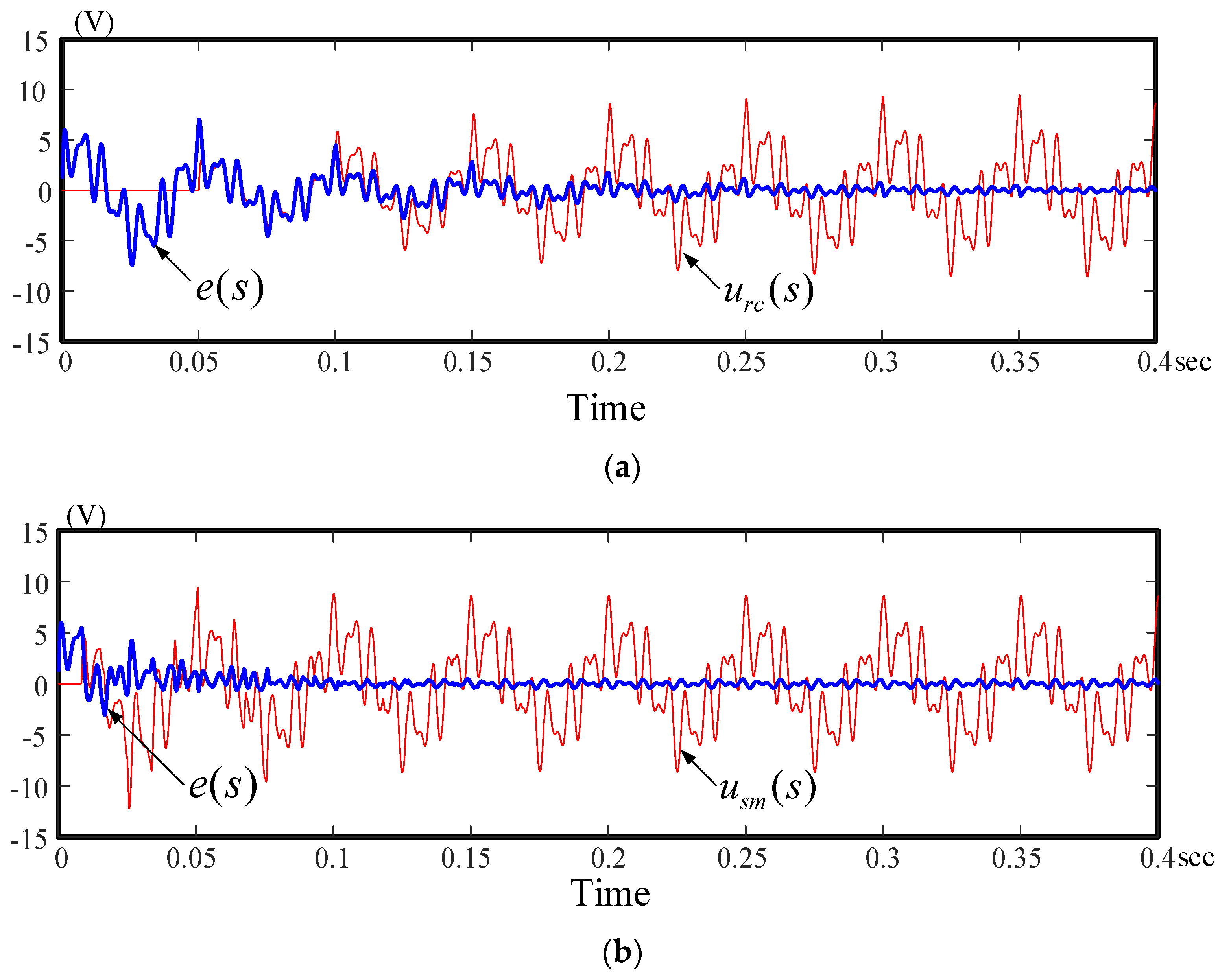
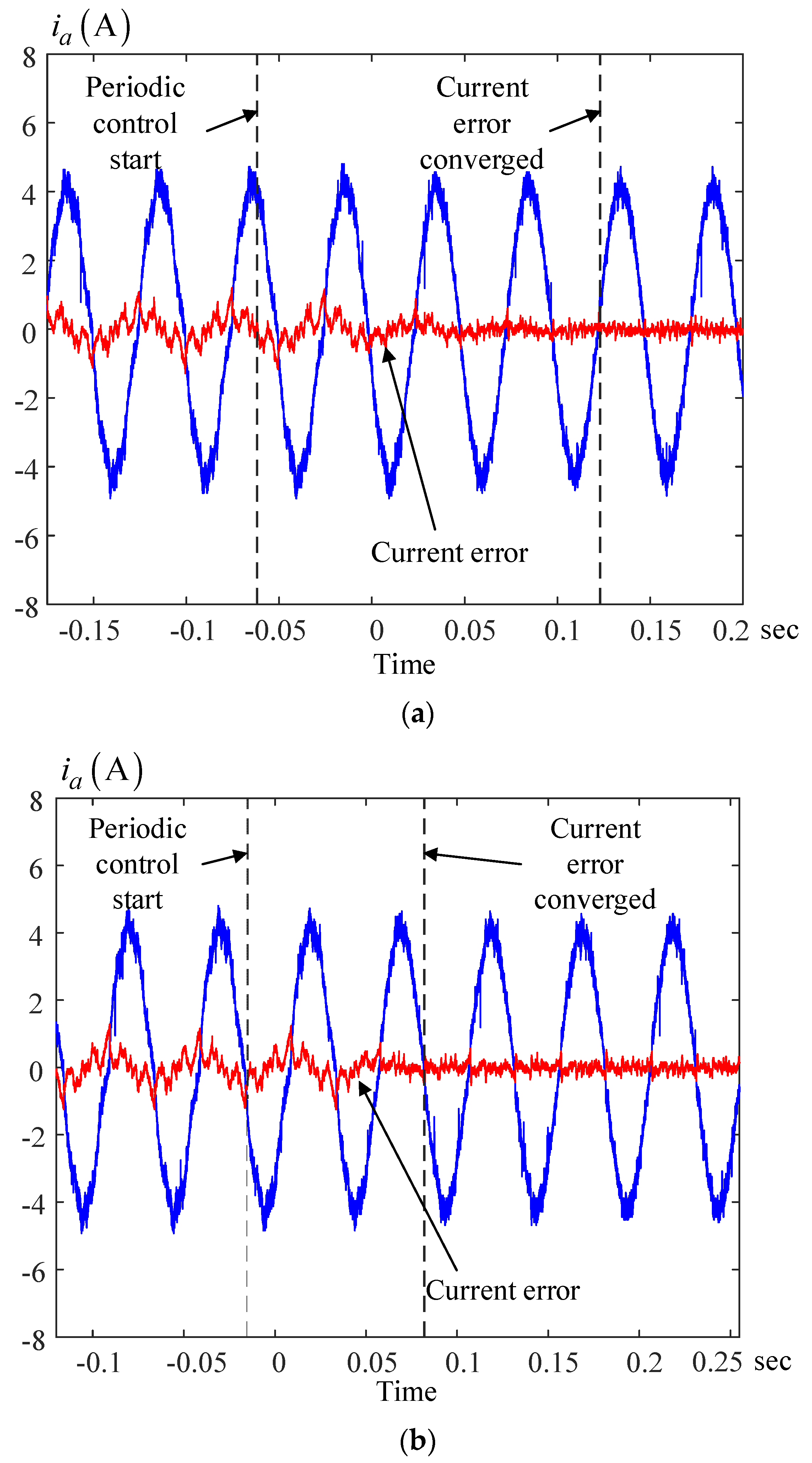
4. Current-Loop Periodic Controller

4.1. Conventional Periodic Current Controller

The block diagram of the CPCs for the current–loop control is shown in Figure 6. First, the d-q axis current commands i d * ( k ) and i q * ( k ) are transferred into the α - β axis current commands i α * ( k ) and i β * ( k ) to prevent the currents from being discontinuous. Then the the α - β axis current commands i α * ( k ) and i β * ( k ) are compared to the α - β axis currents i α ( k ) and i β ( k ) to obtain the α - β axis current errors Δ i α and Δ i β . Next, the α - β axis current errors use CPC and PI controllers to obtain the α - β axis output voltage commands v α * ( k ) and v β * ( k ) . After that, the commands v α * ( k ) and v β * ( k ) pass through space vector pulse width modulation to generate the output a-b-c axis voltages v a ( k ) , v b ( k ) , and v c ( k ) . Finally, the output a-b-c axis voltages produce torque to rotate the IPMSM. A closed-loop IPMSM drive system is thus achieved.

4.2. Current-Loop Selective Harmonic Controller
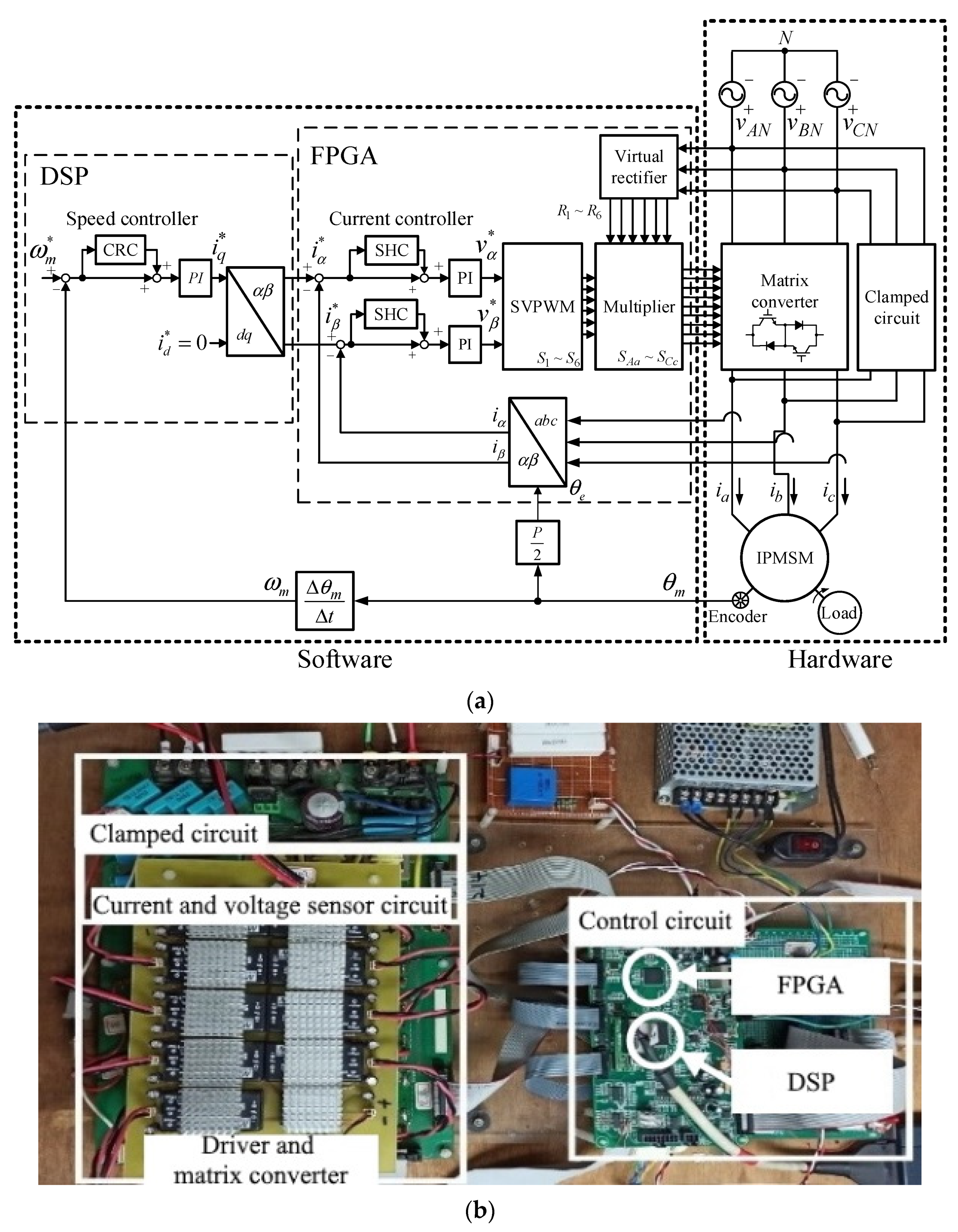
The internal model and the spectrum of the SHC current-loop control are shown in Figure 7a,b. The transfer function is expressed as follows:
u s m ( s ) e ( s ) = G ± m ( s ) = e s T 0 / n ± j ( 2 π m / n ) 1 e s T 0 / n ± j ( 2 π m / n ) = 1 2 + n T 0 1 s j m ω 0 + n 2 T 0 k = 1 s j m ω 0 ( s j m ω 0 ) 2 + n 2 k 2 ω 0 2
where e ( s ) represents Δ i α ( s ) or Δ i β ( s ) , ω 0 is the resonant frequency, and m is the order of the resonant frequency.
By combining half of the G + m ( s ) and half of the G - m ( s ) , one can obtain the G s m ( s ) as follows:
G s m ( s ) = 1 2 ( G + m ( s ) + G m ( s ) ) = 1 2 ( e s T 0 / n + j ( 2 π m / n ) 1 e s T 0 / n + j ( 2 π m / n ) + e s T 0 / n j ( 2 π m / n ) 1 e s T 0 / n j ( 2 π m / n ) )
Equation (30) can be simplified as follows:
G s m ( s ) = cos ( 2 π m / n ) e s T 0 n 1 e 2 s T 0 n 2 cos ( 2 π m / n ) e s T 0 n + 1
The spectrum of the G s m ( s ) is shown as Figure 7b. From Figure 7b, we can observe the spectrum of the transfer function G ± m ( s ) . The selective harmonic generator can produce high gains for the closed-loop current control system at 300 and 420 Hz. As a result, the output currents can track current commands very well at 300 and 420 Hz. If the harmonic current commands are set as zero at 300 and 420 Hz, the real 300 and 420 Hz harmonic currents also can reach near zero. Based on this real internal model, a low-pass filter Q(s) is required, and a phase-lead compensation G f ( s ) is also needed. Then the practical (nk ± m)-order harmonic controller, G s m ( s ) , can be derived as follows [18]:
G s m ( s ) = k m G f ( s ) 2 ( e s T 0 n + j 2 π m n Q ( s ) 1 e s T 0 n + j 2 π m n Q ( s ) + e s T 0 n j 2 π m n Q ( s ) 1 e s T 0 n j 2 π m n Q ( s ) ) = k m G f ( s ) cos ( 2 π m / n ) e s T 0 n Q ( s ) Q 2 ( s ) e 2 s T 0 n 2 cos ( 2 π m / n ) e s T 0 n Q ( s ) + Q 2 ( s )
From Equation (32), one can obtain Figure 8a,b, which shows the discrete-time transfer function of the discrete controller G s m ( z ) as follows:
G s m ( z ) = k s m cos ( 2 π m n ) Q ( z ) z N / n Q 2 ( z ) z 2 N / n 2 cos ( 2 π m n ) Q ( z ) z N / n + Q 2 ( z ) G f ( z )
Figure 8b shows the block diagram of the closed-loop current control system. The basic concept is very clear. When the 300 and 420 Hz harmonic currents appear, the closed-loop periodic current control system has a high gain. As a result, the output current can track current commands very well. If the 300 and 420 Hz harmonic current commands are set as zero, the real 300 and 420 Hz harmonic currents are also near zero. Then, the proposed periodic current controller can effectively reduce the 5th and 7th harmonic currents. From Figure 8b, one can derive the relationship between the output current i ( z ) and input current command i * ( z ) as follows:
i ( z ) = [ 1 + G s m ( z ) ] H ( z ) 1 + G s m ( z ) H ( z ) i * ( z )
The denominator of Equation (34) is described as follows:
1 + G s m ( z ) H ( z ) = z 2 N n + ( k s m G f H ( z ) 2 ) Q ( z ) cos ( 2 π m n ) + ( 1 k s m G f H ( z ) ) Q 2 ( z )
From Equation (35), one can obtain:
1 + G s m ( z ) H ( z ) = ( z N / n α s m e j β s m ) ( z N / n α s m e j β s m )
and
α s m = ± ( 1 - k s m G f H ( z ) ) 1 / 2 Q ( z )
cos ( β s m ) = ± k s m G f H ( z ) 2 2 ( 1 k s m G f H ( z ) ) 1 / 2 cos ( 2 π m / n )
To implement a stable closed-loop system, the poles in Equation (36) are located in a unit circle as follows:
| α s m | < 1
Substituting (37) into Equation (39), one can obtain:
| Q ( e j ω ) | | ( 1 - k s m G f H ( e j ω ) ) 1 / 2 | < 1
Rearranging Equation (40), one can obtain the following equation:
| Q ( e j ω ) | 4 | 1 k s m | G f H ( e j ω ) | e j θ f H ( ω ) | 2 < 1
Substituting | Q ( e j ω ) | 1 into (41), one can derive:
1 2 k s m | G f H ( e j ω ) | cos ( θ f H ( ω ) ) + k s m 2 | G f H ( e j ω ) | 2 < 1
From Equation (42) and by doing some mathematical processes, one can obtain the following condition:
0 < k s m < 2 cos ( θ H + p ω ) | H ( e j ω ) |
The selective harmonic control is then used to eliminate the (nk ± m) order harmonics. In this paper, the (6 k ± 1) order harmonics are eliminated. The parameters, therefore, are chosen as n = 6 and m = 1. In this paper, the sampling time is 100 μs. The delay steps are chosen as N/m, which is 83 steps. The low-pass filter has a bandwidth of 1 kHz and also has a cut-off frequency of 5 kHz. The low-pass filter is a second-order filter. By using MATLAB to do some simulations, one can obtain the parameters of the low-pass filter as a 0 = 0.275, a 1 = 0.45, and a 2 = 0.275. By using the same method as speed-control, the phase lead is selected as p = 1, and the range of the gain is 0 < k s m < 1.406 .
The comparison of a typical case of the CPC and the SHC is shown in Figure 9a,b. The converging speeds of the SHC is 3 times faster than the CPC. However, the steady-state errors of the SHC are not fewer than the CPC. The main reason is that the CPC can provide a wider spectrum than the SHC.

5. Implementation

To verify the developed controller design, an MC-based IPMSM drive system is implemented. Figure 10a shows the implemented motor drive system, and Figure 10b shows a photograph of the hardware circuit. A DSP, type SH 7237, manufactured by Renesas Electronics Corporation, is used as a control center for the speed-loop control by using C-language. An FPGA, type 10M16SAU16917G, manufactured by Intel Corporation, is used to execute current-loop control, coordinated transformation, three-step phase commutation, and SVPWM. The FPGA is developed by using a programmable logic device which can match practical logic circuits [28]. In this paper, the FPGA’s programs are created by using a high-speed hardware description language. The motor is driven by a matrix converter. The currents are detected by Hall-effect sensors and converted via two 12 bit A/D converters. An absolute encoder is used to detect motor positions. The speed-loop sampling interval of the DSP is 1 ms and the current-loop is 100 μs [29].
The parameters of the speed-loop include a PI controller K p = 2.9 and K I = 0.267, as well as a CPC controller, Q(z) = 0.35 z + 0.3 z 1 + 0.35 z 2 , N = 1000, G f ( z ) = z , and k r c = 1.776. In addition, the current-loop includes a PI controller K p = 9.9 and K I = 0.95, as well as a SHC controller, m = 1, n = 6, Q(z) = 0.275 z + 0.45 z 1 + 0.275 z 2 , G f ( z ) = z , and k s m = 1.406, and also a CPC controller, Q(z) = 0.275 z + 0.45 z 1 + 0.275 z 2 , N = 500, G f ( z ) = z , and k r c = 1.406.

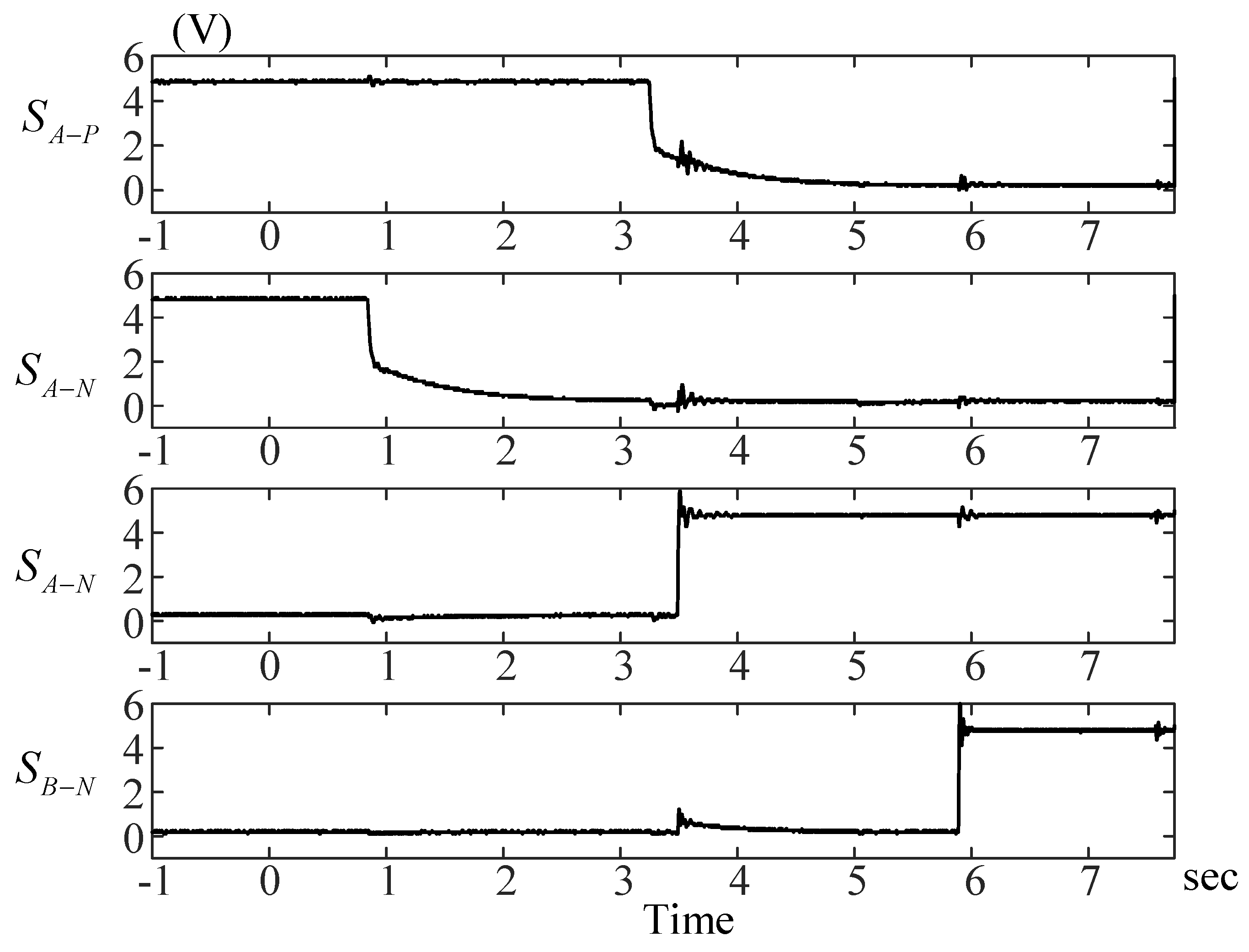
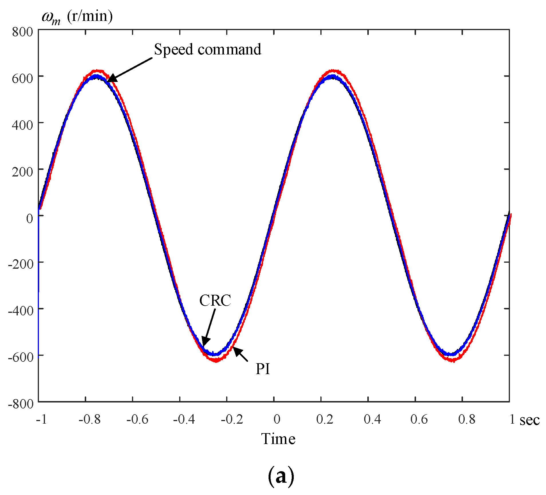
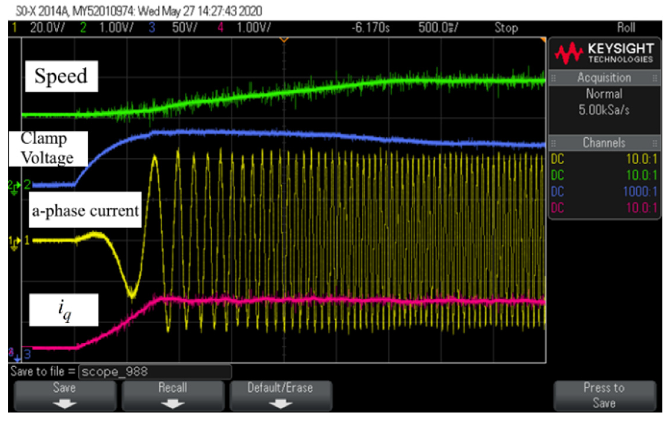
6. Experimental Results

The IPMSM used in this paper is manufactured by TECO Electric Company, type JSMA-PMB-5ABK. The motor is 8-pole with a rated power of 2 kW, a rated current of 9 A, and a rated speed of 2000 r/min. The related parameters are as follows:
The stator resistance is 0.58 Ω , and the inductances include a d-axis inductance of 1.3 mH and a q-axis inductance of 1.7 mH. The inertia is 0.00121 kg·m2. The viscous coefficient is 0.003 N·m s/rad, and the torque constant is 1.14 N·m/A.
Several measured results are demonstrated here to validate the analysis. The parameters of the PI controller are determined by pole assignment. Figure 11, Figure 12, Figure 13, Figure 14 and Figure 15 show several waveforms obtained by using traditional PI controllers and our proposed predictive controllers. Figure 11a demonstrates the comparison of the measured α - axis current command i α * and its current i α , as well as the comparison of the measured β - axis current command i β * and its current i β . Figure 11b shows the current errors Δ i α and Δ i β between the measured α - axis and β -axis current commands and their related measured currents, which both have maximum current errors of ±0.4 A.
Figure 12 shows the measured three-step commutation from the input A-phase to B-phase while the output is connected to the a-phase winding of the IPMSM. The total phase commutation time is 5 μs.
Figure 13a demonstrates the measured sinusoidal speed command and the speed by using the PI and the CPC. Figure 13b shows the measured speed tracking errors between the speed command and the measured speed. The PI controller causes more speed errors than the CPC due to the PI controller’s delayed characteristics.
Figure 14a shows the load disturbance responses at 300 r/min and 4 N·m, with a 1 Hz repetitive load using a PI controller. Figure 14b shows the same case, but uses a CPC.
Figure 15a shows the measured step-input transient responses of the speed. The CPC provides faster responses than the PI controller. Figure 15b demonstrates the measured speed responses at different speed commands from 100 r/min to 1700 r/min. By using a CPC, all of them have linear responses.
Figure 16 and Figure 17 show the measured current waveforms by using periodic current control. Figure 16a,b shows the measured a-phase current and its harmonics at 300 r/min under a 4 N·m load by using a PI controller.
Figure 16c,d shows the same case by using an SHC. By using the SHC, the total harmonics are reduced by 28.6% when compared to the PI controller.
Figure 16e,f shows the same case by using a CPC. The total harmonics are reduced by 32% when compared to the PI controller. From Figure 16a–f, one can conclude that the CPC provides smaller total harmonic distortions than the PI controller and the SHC.
Figure 17a,b shows the measured a-phase currents and their tracking errors. The SHC has a quicker tracking ability than the CPC. According to the measured results, the CPC provides the smallest total current harmonics; however, the SHC provides the fastest converging time for the current-loop control of the IPMSM drive system. The converging time of CPC is 0.18 s, but the converging time of SHC is 0.1 s.
Figure 18 and Figure 19 show the measured results of the FPGA and DSP-based IPMSM drive system. Figure 18a shows the sampling intervals of the speed-loop control and the current-loop control by using only a DSP. The DSP requires 53 μs when the proposed MC-based IPMSM drive system is executed. Figure 18b–e shows the required execution time for the DSP and FPGA when they are used to execute parallel computations. Figure 18b shows the DSP being used as the speed-loop controller, which requires 5 μs. Figure 18c shows the FPGA being used for the conversion of the A/D converter, which requires 8 μs. Figure 18d shows the FPGA being used as the virtual-rectifying control, which requires 1 μs. Figure 18e shows the FPGA being used as the current-loop controller and the SVPWM algorithm, which requires 2.3 μs. From Figure 18b–e, one can obtain that the total execution time of the FPGA is 10.3 μs, which is the summation of the conversion time of the A/D converter, current-loop control time, and SVPWM algorithm time.
Figure 19 shows the measured responses by using a DSP in parallel with an FPGA. As can be observed, the motor drive system provides smooth speed and current responses. The switching frequency of the matrix converter is 50 kHz. In Figure 19, the top waveform is the speed response. The second waveform is the clamped voltage response. The following waveform is the a-phase current response. The bottom waveform shows the q-axis current response of the IPMSM. Those waveforms demonstrate that the proposed DSP in parallel with an FPGA can be successfully used in a silicon carbide based matrix converter motor drive system with a current-loop sampling interval of 10.3 μs. The periodic control works well in this silicon-carbide based matrix-converter IPMSM drive.

7. Conclusions

In this paper, a CPC speed-loop controller, which effectively reduces the speed variations from 80 r/min to 1 r/min when compared to a PI controller, is proposed. In addition, an SHC is implemented as a current-loop controller for an IPMSM drive system to reduce the THD of motor currents from 8.18% to 5.84% when compared to a PI controller. Experimental results show that the proposed methods can effectively remove the periodic harmonic currents and external load disturbances. Two different IPMSM drive systems are implemented and compared. The first IPMSM drive system uses a 32-bit DSP, type SH7237, to execute the control algorithms with a 10 kHz PWM switching frequency. Experimental results of the first IPMSM drive system are shown in Figure 11, Figure 12, Figure 13, Figure 14, Figure 15, Figure 16 and Figure 17. The second IPMSM drive system uses a 32-bit DSP, type SH7237, to execute the speed controller. An FPGA, type 10M16SAU16917G, is also used to execute the current controllers, phase commutation, coordinated transformation, and SVPWM for a silicon-based matrix converter driving an IPMSM drive system with a 50 kHz switching frequency. Experimental results of the second IPMSM drive system are shown in Figure 18 and Figure 19. All of the experimental results demonstrate that both of the IPMSM drive systems with predictive control algorithms provide reduced current harmonics, as well as good transient speeds, load disturbances, and tracking responses.

Author Contributions

Conceptualization, T.-H.L. and K.-H.C.; methodology, T.-H.L. and K.-H.C.; software, K.-H.C. and J.-H.L.; validation, T.-H.L., K.-H.C. and J.-H.L.; formal analysis, T.-H.L., K.-H.C. and J.-H.L.; data curation, K.-H.C. and J.-H.L.; writing—review and editing, T.-H.L. and J.-H.L.; visualization, J.-H.L.; supervision, T.-H.L.; project administration, T.-H.L.; funding acquisition, T.-H.L. All authors have read and agreed to the published version of the manuscript.

Funding

The research was funded by Ministry of Science and Technology, Taiwan, under Grant number MOST 110-2221-E-011-086.

Institutional Review Board Statement

Not applicable.

Informed Consent Statement

Not applicable.

Data Availability Statement

Not applicable.

Acknowledgments

This paper is supported by the MOST, Taiwan, under grant 109-2221-E-011-05.

Conflicts of Interest

The authors declare no conflict of interest.

Nomenclature

S 1 S 9 bidirectional switches of matrix converter
V d c virtual DC-link voltage
V A N - V C N input three-phase voltages of matrix converter
v a - v c output three-phase voltages of matrix converter
R R 1 R R 6 bidirectional switches of virtual rectifier
I N 1 I N 6 unidirectional switches of virtual inverter
d d t differential operator
i d s , i q s d-q axis currents of IPMSM
v d s , v q s d-q axis voltages of IPMSM
L d s , L q s d-q axis inductances of IPMSM
R s resistance of IPMSM
P pole number of IPMSM
λ m flux linkage of permanent magnet material in IPMSM
T e total torque
ω r m mechanical rotor speed of IPMSM
ω e electrical rotor speed of IPMSM
θ r m mechanical rotor position of IPMSM
θ e electrical rotor position of IPMSM
γ d polynomial of the multi sinusoids
ω i different frequencies
LLaplace transformation
K h control gain
φ h phase-lead angle
ss-domain
zz-domain
ω 0 resonant frequency
ω h h times of resonant frequency
h harmonic order
G r c transfer function of classical periodic controller
T 0 period of high-frequency signal
N delay times
k r c constant gain of classical periodic controller
Q transfer function of low-pass filter
G f Phase-lead compensator
Hclosed-loop transfer function using PI controller
θ H phase angle
θ f H summation of θ H and p ω
a 0 a 2 parameters of low-pass filter
u r c , u s m input of periodic controller
i α α -axis current
v α α -axis voltage
i β β -axis current
v β β -axis voltage
G ± m transfer function of selective harmonic periodic controller
G s m combined transfer function
k s m DC gain of selective harmonic periodic controller
K P proportional gain of PI controller
K I integral gain of PI controller
α s m pole
Δ ω r mechanical speed error
Δ ω r 0 initial value of mechanical speed error
G p transfer function of plant
G c transfer function of PI control
G h transfer function of an IMP-based resonant controller

References

  1. Gao, Q.; Asher, G.M.; Sumner, M.; Empringham, L. Position estimation of a matrix-converter-fed AC PM machine from zero to high speed using PWM excitation. IEEE Trans. Ind. Electron. 2009, 56, 2030–2038. [Google Scholar]
  2. Chen, Y.; Liu, T.H.; Cuong, N.M. Implementation of sensorless DC-link capacitorless inverter-based interior permanent magnet synchronous motor drive via measuring switching-state current ripples. IET J. 2016, 10, 197–207. [Google Scholar] [CrossRef]
  3. Dasika, J.D.; Saeedifard, M. A fault-tolerant strategy to control the matrix converter under an open-switch failure. IEEE Trans. Ind. Electron. 2015, 62, 680–691. [Google Scholar] [CrossRef]
  4. Brunson, C.; Empringham, L.; Lillo, L.D. Open-circuit fault detection and diagnosis in matrix converters. IEEE Trans. Power Elecron. 2015, 30, 2840–2847. [Google Scholar]
  5. Wheeler, P.W.; Clare, J.; Empringham, L. Enhancement of matrix converter output waveform quality using minimized commutation times. IEEE Trans. Electron. 2004, 51, 240–244. [Google Scholar] [CrossRef]
  6. Wheeler, P.W.; Clare, J.C.; Empringham, L.; Bland, M.; Apap, M. Gate drive level intelligence and current sensing for matrix converter current commutation. IEEE Trans. Ind. Electron. 2002, 49, 382–389. [Google Scholar] [CrossRef]
  7. Xiao, D.; Rahman, M.F. Sensorless direct torque and flux controlled IPM synchronous machine fed by matrix converter over a wide speed range. IEEE Trans. Ind. Inform. 2013, 9, 1855–1867. [Google Scholar] [CrossRef]
  8. Gong, Z.; Zheng, X.; Zhang, H.; Dai, P.; Wu, X.; Li, M. A QPR-based low-complexity input current control strategy for the indirect matrix cinverters with unity grid power factor. IEEE Access 2019, 2019, 38766–38777. [Google Scholar] [CrossRef]
  9. Wisniewski, R.; Bazydlo, G.; Szczesniak, P.; Wojnakowski, M. Petri net-based specification of cyber-physical systems oriented to control direct matrix converters with space vector modulation. IEEE Access 2019, 2019, 23407–23420. [Google Scholar] [CrossRef]
  10. Kumar, V.; Joshi, R.R.; Bansal, R.C. Optimal control of matrix-converter-based WECS for performance enhancement and efficiency optimization. IEEEE Trans. Energy Conver. 2009, 24, 264–273. [Google Scholar] [CrossRef]
  11. Xia, C.; Yan, Y.; Song, P.; Shi, T. Voltage disturbance rejection for matrix converter-based PMSM drive system using internal model control. IEEE Trans. Ind. Electron. 2012, 59, 361–372. [Google Scholar]
  12. Yao, W.; Liu, J.; Lu, Z. Distributed control for the modular multilevelmatrix converter. IEEE Trans. Power Electron. 2019, 34, 3775–3788. [Google Scholar] [CrossRef]
  13. Monteiro, J.; Silva, J.F.; Pinto, S.F.; Palma, J. Linear and sliding-mode controller matrix converter-base unified power controllers. IEEE Trans. Power Electron. 2014, 29, 3357–3367. [Google Scholar]
  14. Formentini, A.; Trentin, A.; Marchesoni, M.; Zanchetta, P.; Wheeler, P. Speed finite control set model predictive control of a PMSM fed by matrix converter. IEEE Trans. Ind. Electron. 2015, 62, 6786–6796. [Google Scholar] [CrossRef]
  15. Shigeuchi, K.; Xu, J.; Shimosato, N.; Sato, Y. A modulation method to realize sinusoidal line current for bidirectional isolated three-phase AC/DC dual-active-bridge converter based on matrix converter. IEEE Trans. Power Electron. 2020, 36, 6015–6029. [Google Scholar] [CrossRef]
  16. Lei, J.; Feng, S.; Zhou, B.; Nguyen, H.N.; Zhao, J.; Chen, W. A simple modulation scheme with zero common-mode voltage and improved efficiency for direct matrix converter-fed PMSM drives. IEEE J. Emerg. Sel. Top. Power Electron. 2020, 8, 3712–3722. [Google Scholar] [CrossRef]
  17. Szczepankowski, P.; Wheeler, P.; Bajdecki, T. Application of analytic signal and smooth interpolation in pulsewidth modulation for conventional matrix converters. IEEE Trans. Ind. Electron. 2020, 67, 10011–10023. [Google Scholar] [CrossRef]
  18. Li, Y.; Qiu, L.; Zhi, Y.; Yan, G.; Zhang, J.; Ma, J.; Fang, Y. An overmodulation strategy for matrix converter under unbalanced input voltages. IEEE Access 2021, 2021, 2345–2356. [Google Scholar] [CrossRef]
  19. Deng, W.; Li, S. Direct torque control of matrix converter-fed PMSM drives using multidimensional switching table for common-mode voltage minimization. IEEE Trans. Power Electron. 2021, 36, 683–690. [Google Scholar] [CrossRef]
  20. Fang, F.; Tian, H.; Li, Y. Coordination control of modulation index and phase shift angle for current stress reduction in isolated AC-DC matrix converter. IEEE Trans. Power Electron. 2021, 36, 4585–4596. [Google Scholar] [CrossRef]
  21. Urrutia, M.; Cardenas, R.; Clare, J.C.; Watson, A. Circulating current control for the modular multilevel matrix converter based on model predictive control. IEEE J. Emerg. Sel. Top. Power Electron. 2021, 9, 6069–6085. [Google Scholar] [CrossRef]
  22. Mir, T.N.; Singh, B.; Bhat, A.H. FS-MPC-Based speed sensorless control of matrix converter fed induction motor drive with zero common mode voltage. IEEE Trans. Ind. Electron. 2021, 68, 9185–9195. [Google Scholar] [CrossRef]
  23. Fang, F.; Tian, H.; Li, Y. Finite control set model predictive control for AC-DC matrix converter with virtual space vectors. IEEE Jour. Emerg. Select. Top. Power Electron. 2021, 9, 616–628. [Google Scholar] [CrossRef]
  24. Trzynadlowski, A.M. Introduction to Modern Power Electronics, 2nd ed.; Wiley: Hoboken, NJ, USA, 2010. [Google Scholar]
  25. Rogers, E.; Galkowski, K.; Owens, D.H. Control Systems Theory and Applications for Linear Repetitive Processes; Springer: Berlin/Heidelberg, Germany, 2007. [Google Scholar]
  26. Goodwin, G.C.; Graebe, S.F.; Salgado, M.E. Control System Design; Prentice-Hall: Hoboken, NJ, USA, 2001. [Google Scholar]
  27. Zhou, K.; Wang, D.; Yang, Y.; Blaabjerg, F. Periodic Control of Power Electronic Converters; The Institute of Engineering and Technology: London, UK, 2016. [Google Scholar]
  28. Unsalan, C.; Tar, B. Digital System Design with FPGA-Implementation Using Verilog and VHDL; McGraw Hill: New York, NY, USA, 2017. [Google Scholar]
  29. Toliyat, H.A.; Compbell, S. DSP-Based Electromechanical Motion Control; CRC Press: New York, NY, USA, 2004. [Google Scholar]
Figure 1. The matrix-converter configuration: (a) main circuit; (b) equivalent circuit; (c) virtual DC-link voltage.
Energies 14 08073 g001aEnergies 14 08073 g001b
Figure 2. The continuous-time of the periodic signal generator: (a) internal model; (b) spectrum diagram.
Energies 14 08073 g002aEnergies 14 08073 g002b
Figure 3. The periodic controller of the speed-loop: (a) continuous controller G r s ( s ) ; (b) discrete controller G r s ( z ) ; (c) closed-loop speed-control.
Energies 14 08073 g003aEnergies 14 08073 g003b
Figure 4. The boundary of control parameters: (a) phase lead; (b) gain.
Energies 14 08073 g004aEnergies 14 08073 g004b
Figure 5. The periodic control: (a) block diagram; (b) speed error Δ ω r ( z ) ; (c) periodic input u r c ( z ) ; (d) total control input.
Energies 14 08073 g005
Figure 6. The CPC current-loop control for an IPMSM drive.
Energies 14 08073 g006
Figure 7. Continuous time-domain selective harmonic generator: (a) internal model; (b) spectrum at 50 Hz.
Energies 14 08073 g007
Figure 8. The block diagram of selective harmonic control: (a) selective harmonic generator; (b) block diagram.
Energies 14 08073 g008
Figure 9. Responses between different controllers of current-loop control: (a) CPC; (b) SHC.
Energies 14 08073 g009
Figure 10. The implemented system: (a) block diagram; (b) hardware circuit.
Energies 14 08073 g010
Figure 11. The measured currents at 300 N·m with a 3 N·m load: (a) comparisons; (b) α - β axis current errors.
Energies 14 08073 g011
Figure 12. The measured waveforms of three-step commutation.
Energies 14 08073 g012
Figure 13. The measured sinusoidal speed responses: (a) responses; (b) tracking errors.
Energies 14 08073 g013aEnergies 14 08073 g013b
Figure 14. The measured repetitive disturbance responses: (a) PI controller; (b) CPC.
Energies 14 08073 g014aEnergies 14 08073 g014b
Figure 15. The measured transient responses: (a) single step-input; (b) different step-input commands.
Energies 14 08073 g015aEnergies 14 08073 g015b
Figure 16. The measured a-phase currents and their harmonics: (a) current using PI; (b) harmonics using PI; (c) current using SHC; (d) harmonics using SHC; (e) current using CPC; (f) harmonics using CPC.
Energies 14 08073 g016aEnergies 14 08073 g016bEnergies 14 08073 g016c
Figure 17. The measured currents and current errors: (a) CPC; (b) SHC.
Energies 14 08073 g017
Figure 18. The measured computation time: (a) using only a DSP; (b) DSP speed-loop computation; (c) FPGA A/D conversion; (d) FPGA virtual rectifying; (e) FPGA current-loop and SVPWM.
Energies 14 08073 g018
Figure 19. The measured responses using a silicon-carbide matrix-converter with a 50 kHz switching frequency.
Energies 14 08073 g019
Table 1. Main control methods of matrix converter-based AC drives.
AuthorsReference NumbersControl MethodsPublished Years
Kumar et al.[10]Optimal control2009
Xia et al.[11]Internal model control2012
Monteiro et al.[13]Sliding mode control2014
Formentini et al.[14]Predictive control2015
Gong et al.[8]Quasi-proportional resonance2019
Urrutia et al.[21]Predictive control2021
Mir et al.[22]Predictive control2021
Fang et al.[23]Predictive control2021
Publisher’s Note: MDPI stays neutral with regard to jurisdictional claims in published maps and institutional affiliations.

