Modeling, Simulation, and Analysis of a Variable-Length Pendulum Water Pump

Abstract

Due to the long-term problem of electricity and potable water in most developing and undeveloped countries, predominantly rural areas, a novelty of the pendulum water pump, which uses a vertically excited parametric pendulum with variable-length using a sinusoidal excitation as a vibrating machine, is presented. With this, more oscillations can be achieved, reducing human effort further and having high output than the existing pendulum water pump with the conventional pendulum. The pendulum, lever, and piston assembly are modeled by a separate dynamical system and then joined into the many degrees-of-freedom dynamical systems. The present work includes friction while studying the system dynamics and then simulated to verify the system’s harmonic response. The study showed the effect of the pendulum length variability on the whole system’s performance. The vertically excited parametric pendulum with variable length in the system is established, giving faster and longer oscillations than the pendulum with constant length. Hence, more and richer dynamics are achieved. A quasi-periodicity behavior is noticed in the system even after 50 s of simulation time; this can be compensated when a regular external forcing is applied. Furthermore, the lever and piston oscillations show a transient behavior before it finally reaches a stable behavior.

1. Introduction

According to Canada’s government, about 40% of the world population does not have a pleasing way of getting sanitary water, which is hugely affected by the developing countries where up to 80% of illness in such areas is caused by inadequate water and sanitation [1]. Furthermore, Ref. [2] shows that more than a billion people in developing countries have insufficient clean water due to deprivation, change in climate, and bad governance. This leads to several issues such as under supply of drinking water, deficient structure to get water supply, swamp, droughts, and contamination of rivers as well as large dams [2]. In addition, people entail good water for livelihood, essential care, farming or agriculture, manufacturing, and trade. According to the 2019 UN World Development report, stated about four billion people, which is virtually two-thirds of the world population, encounter severe water scarcity at least one month in a year [2].

With the long-term problem of electricity and potable water in most developing and underdeveloped countries, especially in rural areas, more research needs to be done in areas that can positively affect their lives. One such area is the availability and accessibility of water for domestic, agricultural, and even industrial uses. There is a need to modify the existing water pump, such as the conventional hand water pumps. These rural dwellers can access good water even without electricity for the pumping (for some types of pumps). A pendulum can be used to provide the initial force for the pumping process in a reciprocating water pump [3,4]. With this principle, more water liters can be pumped with little effort since more energy can be overcome by small or little effort on the pendulum, thereby increasing the whole system’s efficiency [5].

The importance of pendulum water pumps is that they significantly reduce to a minimum the human strain, making the water pumps easy to operate [6,7]. The pendulum is occasionally pushed with little effort, even with the fingers. It keeps the pumping continuous, unlike an ordinary hand pump, which always requires a load with significant steps [8]. A normal person can only make use of the hand pump for a few minutes. When pressed, water stops pumping. The situation is different from the pendulum water pump, i.e., a little pressure is needed to push the pendulum to keep changing and keep it oscillating for several hours without getting tired.

In [9], authors presented a three-dimensional model and a fabricated water hand pump with a pendulum. The pendulum’s energy was analyzed based on the pendulum’s kinetic and potential energy without further algorithms. In addition, 1200 L per hour of water discharge were observed using the pump with a pendulum. We noted that system dynamics need to be studied deeper to improve system efficiency and control for better performance and other research purposes.

In [8], a design, as well as the development of a pendulum-operated water pump, are presented. The mode of operation of the pendulum-operated water pump is based on defining the functions of all parts separately, but a mathematical model is not presented.

A fabricated set-up of an analytical design of a pendulum hand pump using Creo is covered by [6]. The design calculations were performed manually. The analyses show that the set-up has $70\%$ efficiency at the initial angle of the pendulum, $39\%$ efficiency when the pendulum is at 60${}^{\circ }$ with the lever, and $25.5\%$ efficiency when the pendulum angle is at 0 or 90${}^{\circ }$ with the lever. Similarly, experimental statistics from a test rig, including validation of the dual-medium pressurizer’s energy transmission strategy, are considered in [10]. An onshore pendulum’s wave energy converter test rig was built for validation. It uses a hydraulic cylinder as a replacement for the wave that deploys a force on the pendulum. The overall result of the simulation shows a similar response to the experimental results.

In [11], authors designed and fabricated a pendulum hand pump. Parts of the functions were stated, the advantages and disadvantages of the pendulum pumps, the working principle, and its applications. The equations of motion need to be derived and solved numerically to allow further analysis to achieve better system performance. 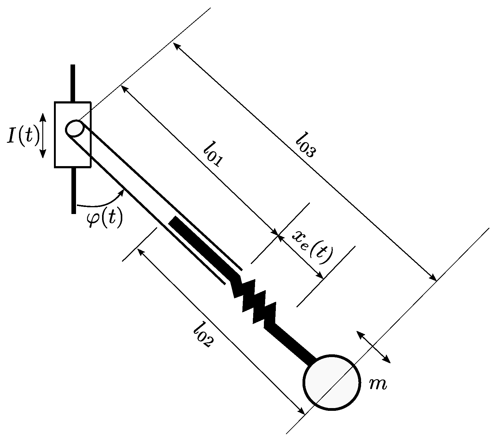A kinematic approach in the theoretical analysis of a pendulum hand pump dynamics is presented in [5] where a nonlinear pendulum model is used to power the lever and the piston model for the applied excitation force to the pendulum. It is observed that satisfactory results are obtained where the frequency of excitation is greater than the pendulum’s natural frequency of the model. In [5], we find the equation of the pendulum model as follows:

$$\ddot{\phi }+\frac{g}{l}sin\phi =f\left(t\right),$$

(1)

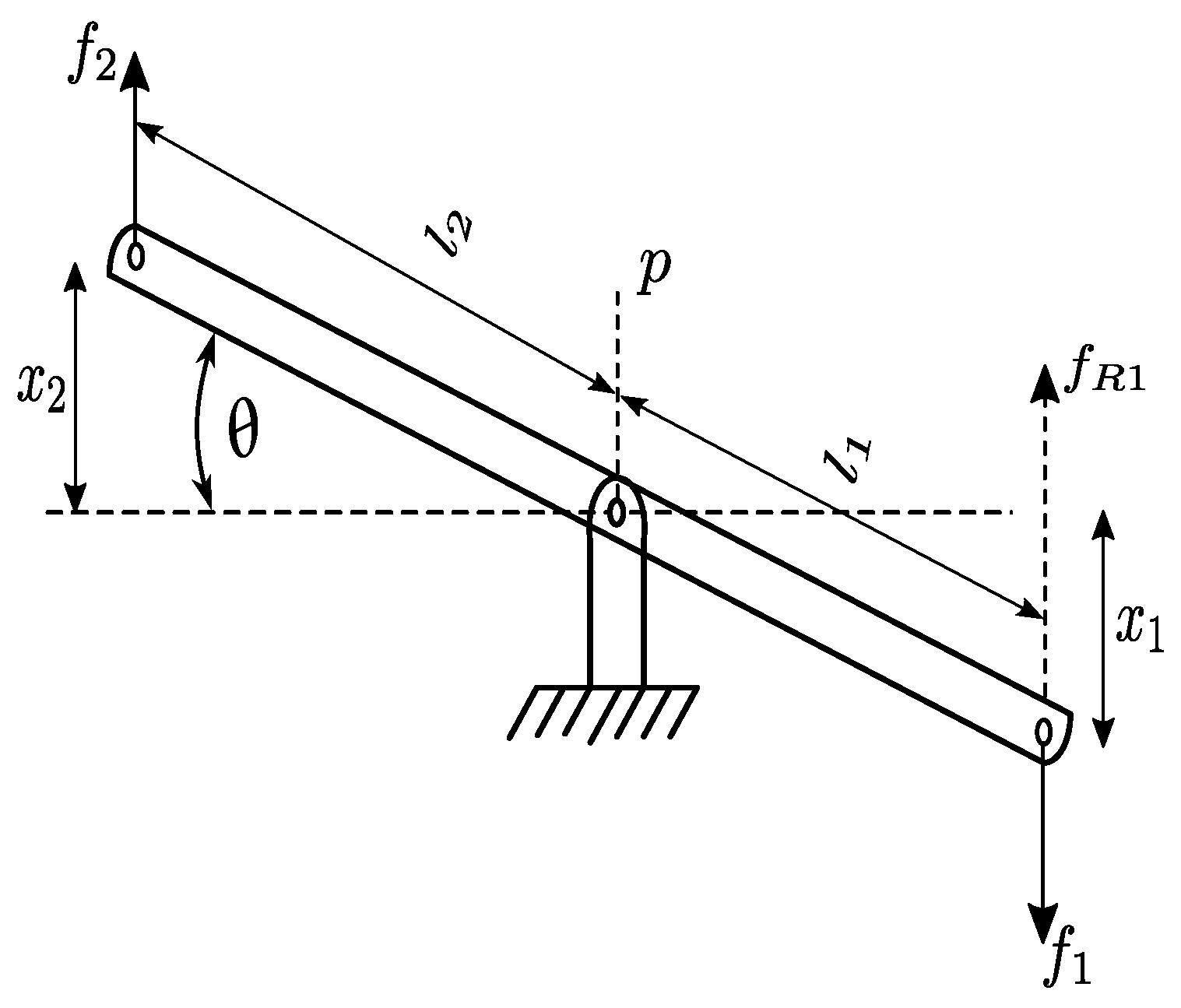
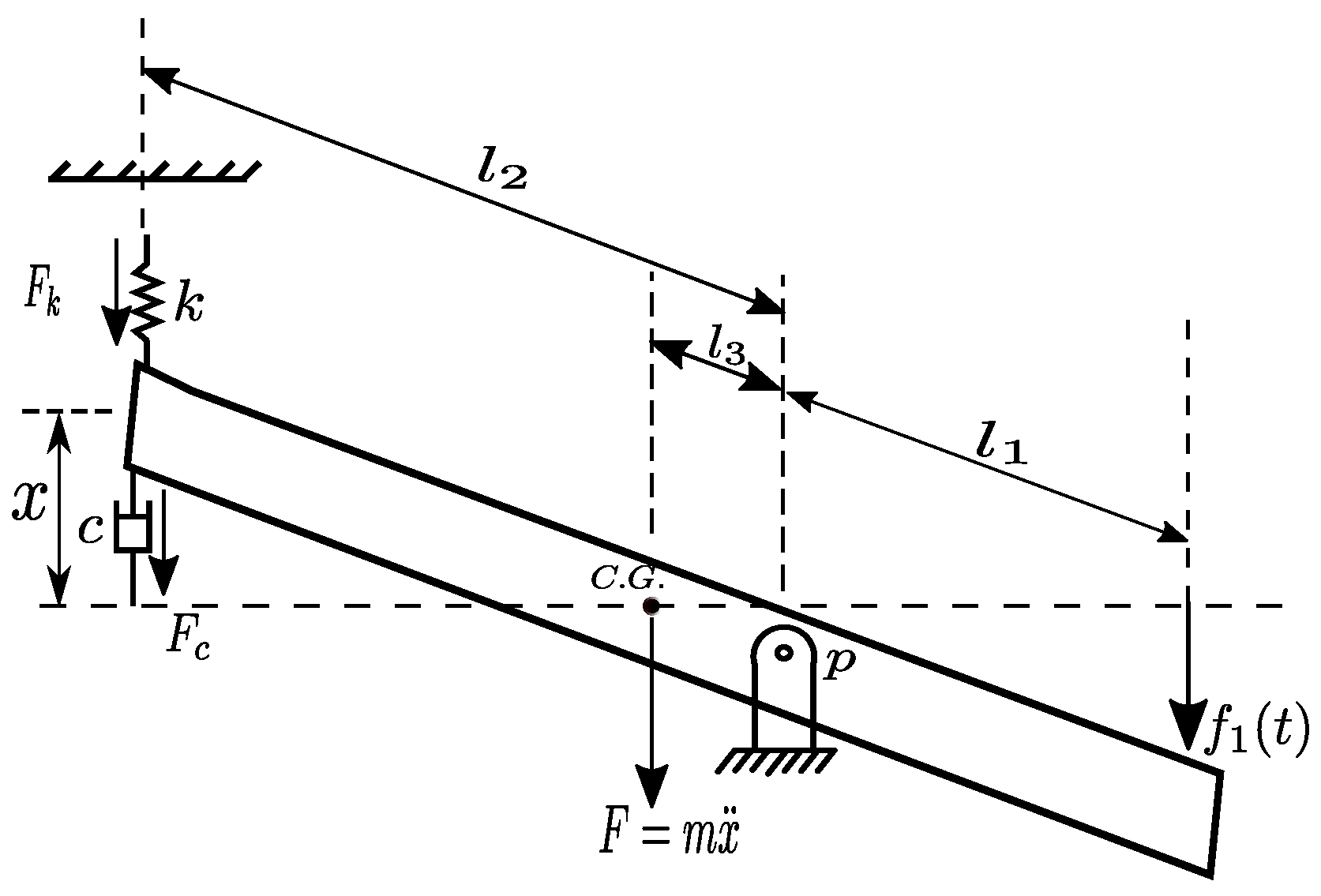
and the equation of the lever and piston as below

$$\ddot{x}=\frac{3}{m}\left(f_1\left(t\right)\frac{l_1}{l_2}-b\dot{x}-kx\right),$$

(2)

where: $\phi$—pendulum’s angular displacement, g—acceleration due to gravity, l—length of the pendulum, $f\left(t\right)$—input force from the pendulum model given as $f\left(t\right)=f_{0}cos\left(\omega t\right)$; $f_0$—forcing excitation amplitude, $\omega$—excitation frequency, m—the mass of the lever and piston model, k—spring constant, b—viscous damping constant, $l_1$—distance from the input force and the lever point of pivot, P, $l_2$—distance from point k and P, and $f_1\left(t\right)=sin\phi$. 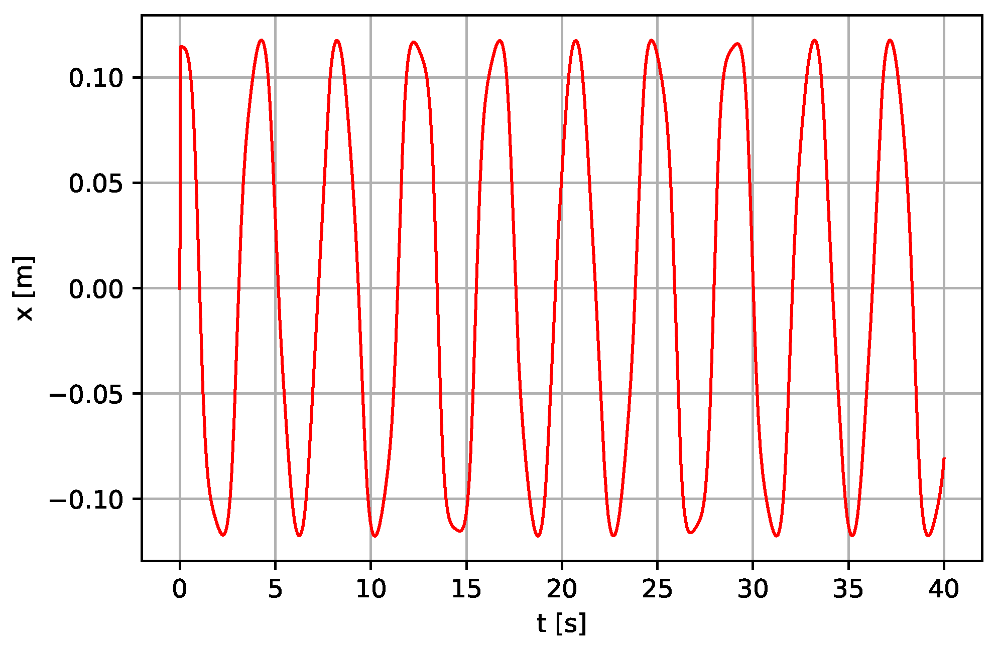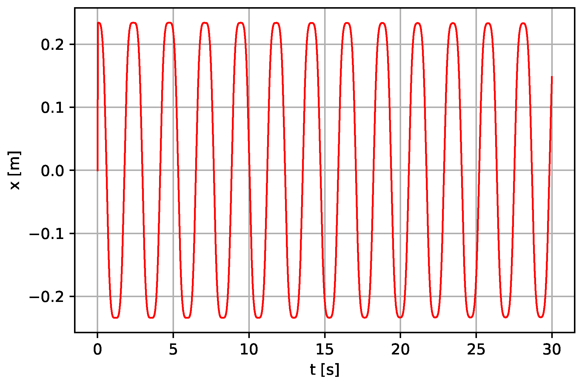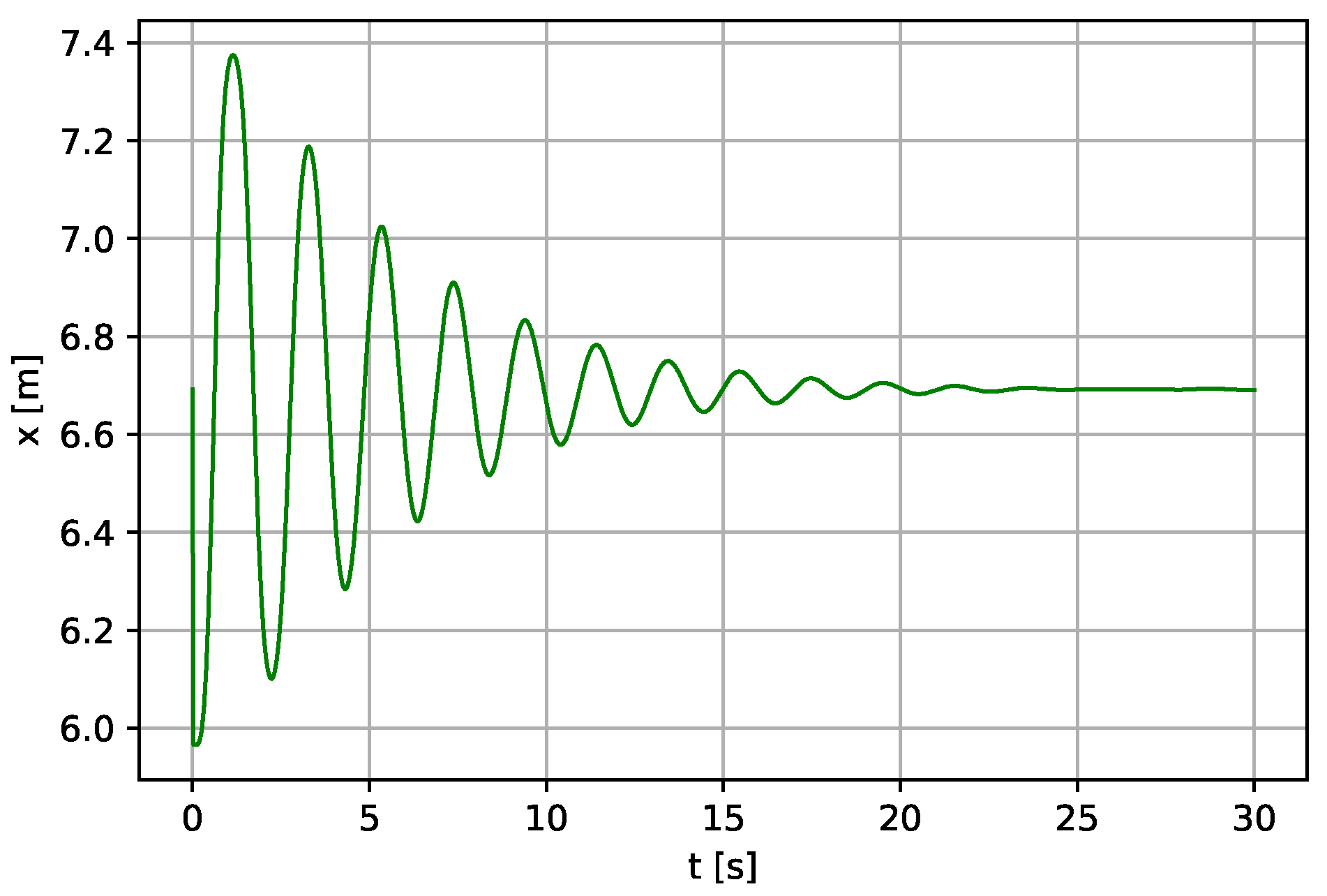Integrating numerically, Equation (7) yields the piston displacement, x. 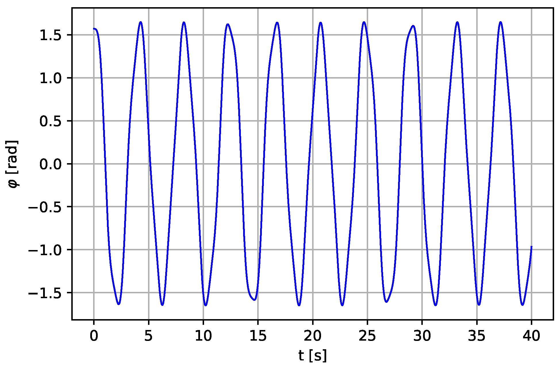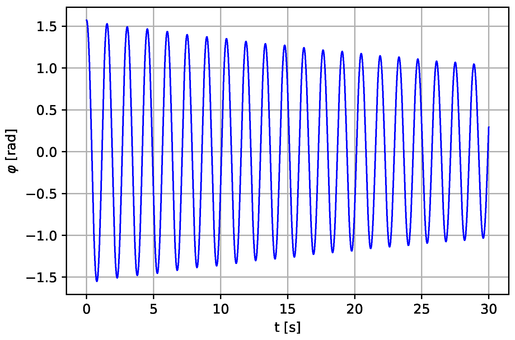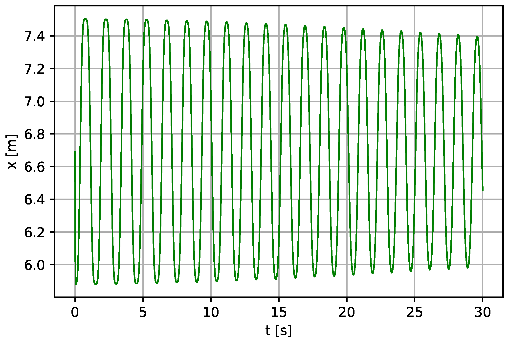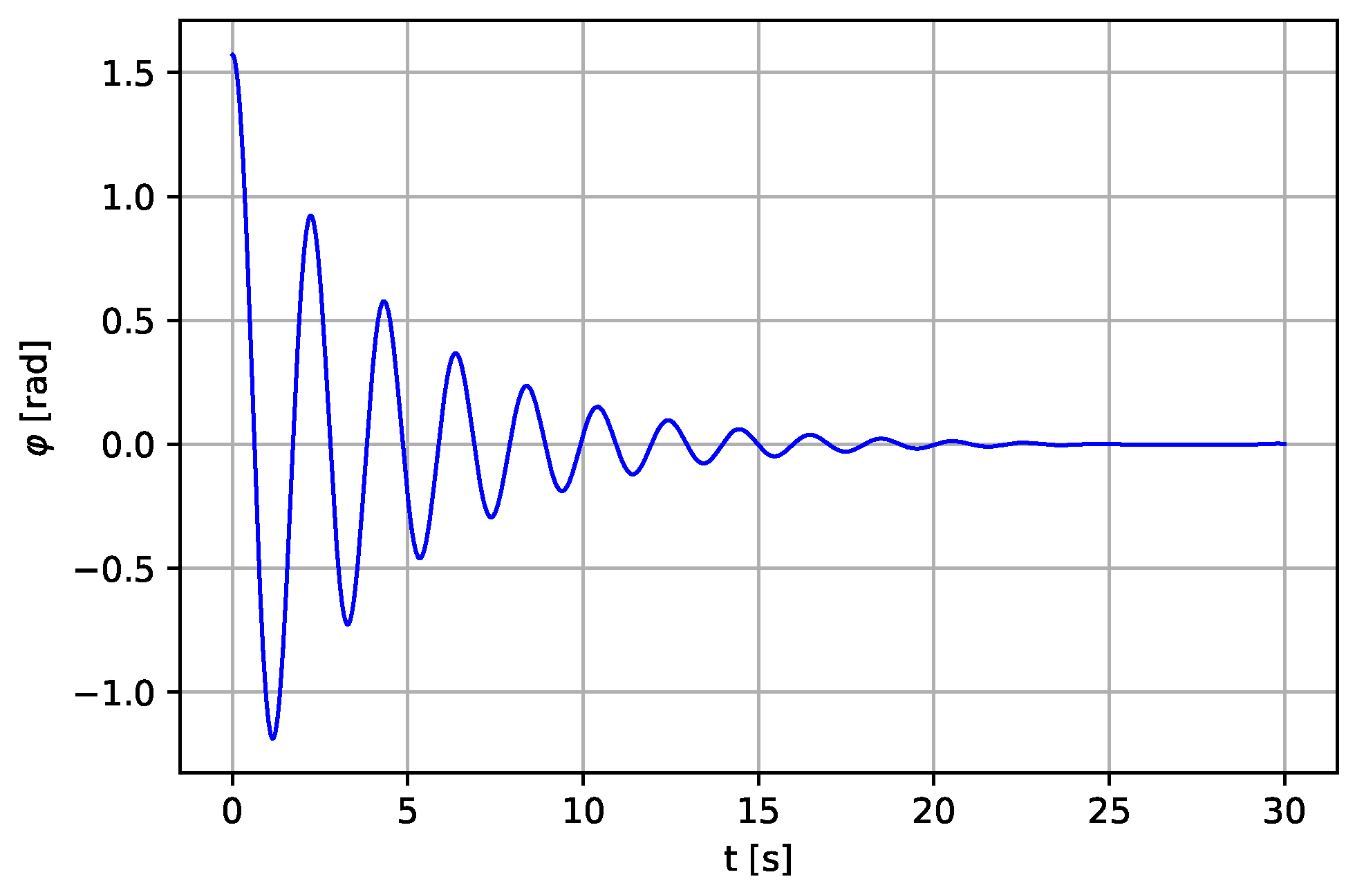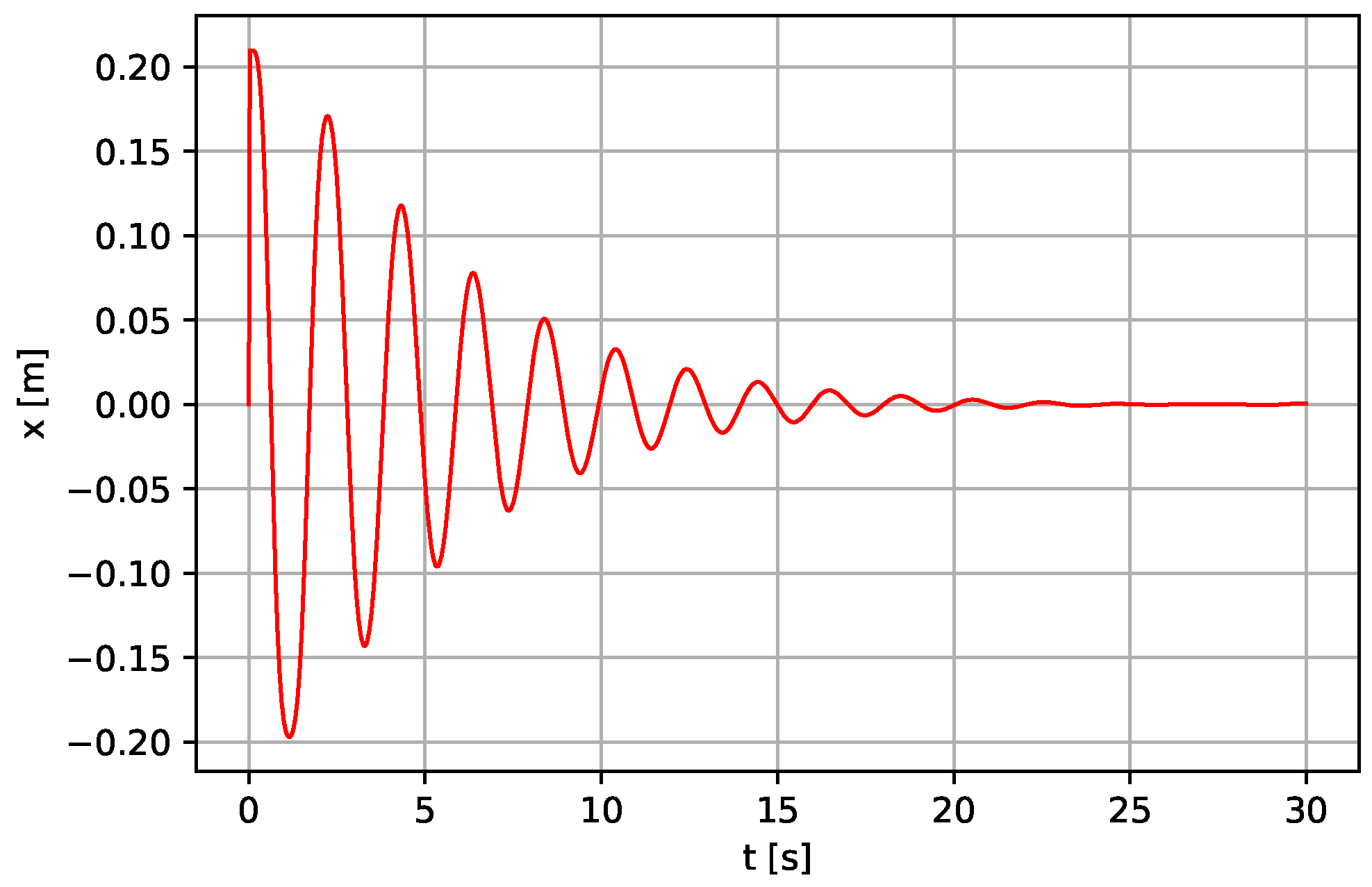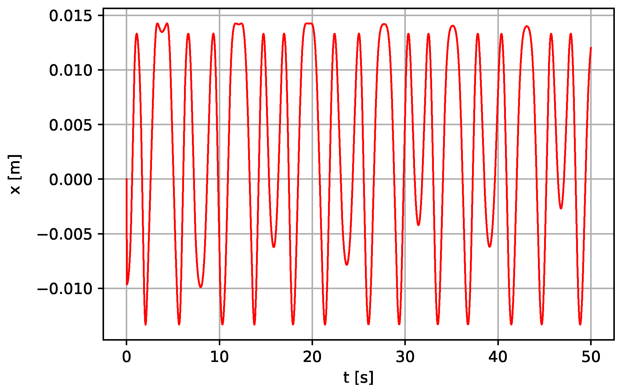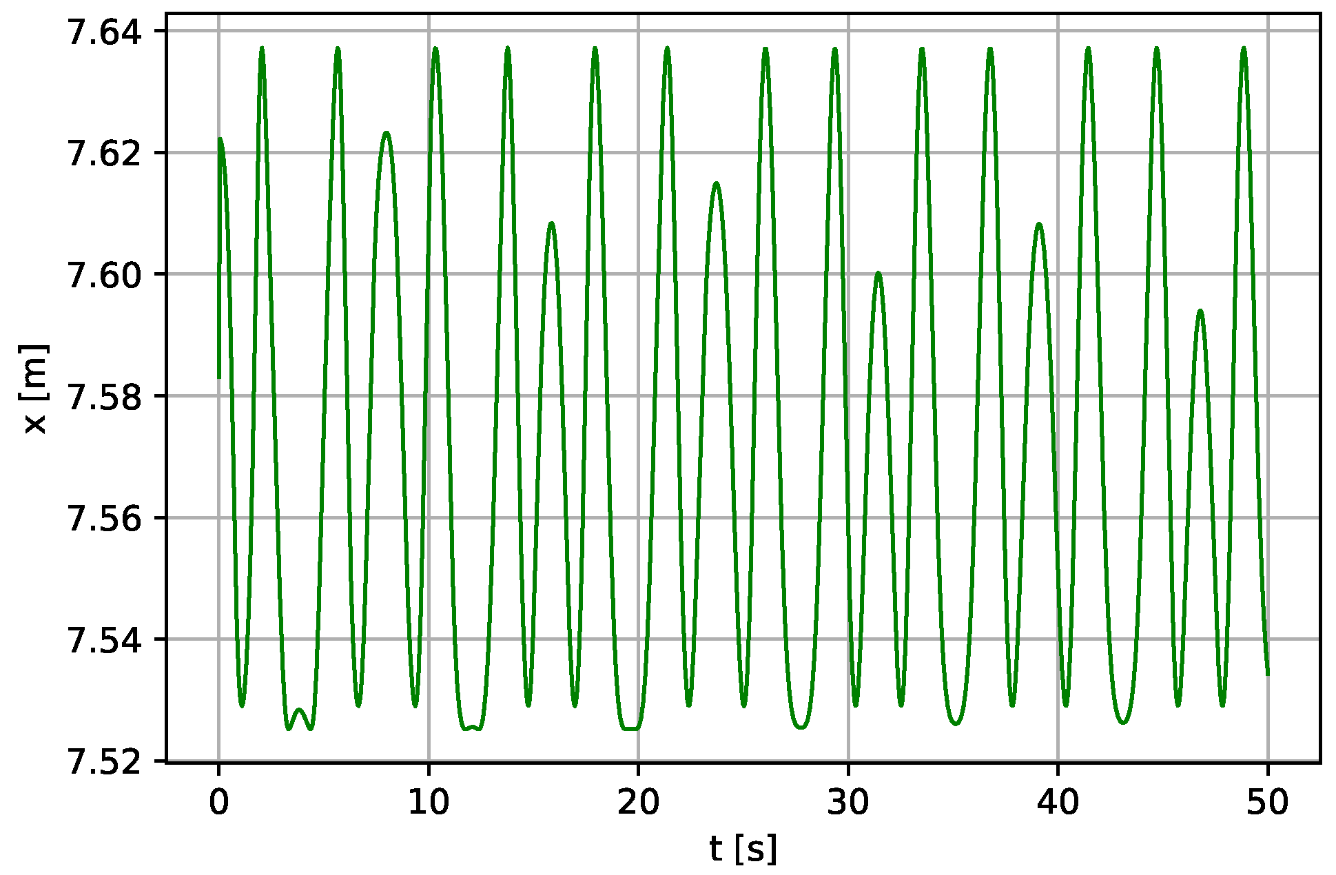Using the same parameters presented in [5] ($l=3$ m, $\omega =5$ rad/s, $f_0=3$ m, $l_1=0.4$ m, $l_2=0.6$ m, $l_3=\frac{1}{3}{l}_2$, $k=5$ N·m⁻¹, $b=1$ N·s·m⁻¹, $m=4\mathrm{kg}$), we use the proposed numerical approach of our modified system to solve Equations (1) and (2), and we have the numerical solution as shown in Figure 1 and Figure 2, which is very similar to the ones presented in [5].

The study needs a pivotal and in-depth analysis of fluid mechanics, and the pendulum’s length can also affect the system’s performance.

To further reduce the human effort, we proposed to use a pendulum with a variable-length model instead of the conventional pendulum. This modification would give a faster and longer oscillation, which will, in turn, result in more rapid pumping of fluid since the variable-length pendulum can undergo a quicker and longer oscillation, as presented by the following authors: Ref. [12] derived the differential equations of dynamics for both the first and the second mutation from the sum of kinetic and potential energy for a rigid pendulum’s two and three degrees of freedom. It was observed that a successive expansion in the forms of representation of the energy is introduced. The largest Lyapunov exponent was used to classify the system based on computational analysis. The phase planes and the Poincaré maps show some homogeneous dynamic patterns, such as quasi-periodic and chaotic motions. Refs. [13,14], the Euler–Lagrange equation, and the Rayleigh dissipation function are used to derive the equation for a three-degree of freedom pendulum system. The numerical results reveal that a variable-length spring pendulum hung from the occasionally forced slider can demonstrate quasi-periodicity and chaotic motions in a resonance condition. Furthermore, near the resonance, linking bodies on the system dynamics could lead to unforeseeable dynamical comportment.

Krasilnkov presents in [15] the variable-length pendulum harmonic oscillations, which depend on the length of the pendulum. Lyapunov exponents, bifurcation diagrams, and the Poincaré maps situated on phase plane diagrams were used to inspect the system behavior. It was concluded that the system exhibited chaotic properties in the domain of higher-level stability. A control scheme for a vertically excited parametric pendulum with variable length is presented in [16]. It offers two energy sources: a vibrating machine and sea waves simulated by a stochastic process [16]. For the pendulum to be controlled, a telescopic adjustment of the pendulum length [16] is used during the motion. The numerical results show favorable terms for energy harvesting. Steady revolutions can be attained irrespective of the forcing factors and for all established initial conditions. It is concluded that it is hard to attain stable rotation due to the high reliance of the dynamical system on parameters that causes the forcing and the initial conditions. However, the controlled pendulum can reach stable rotations if the threshold velocity is sufficiently selected to modulate the control operation.

In this work, we present the following:

• The mathematical model and simulation results of the variable-length pendulum water pump were performed. The equations were solved using the Runge–Kutta method with 5th order adaptive step size.
  A vertically excited parametric pendulum with variable length [16] is used instead of the conventional pendulum with constant length, minimizing human effort with increasing output of water or liquid from the pump outlet.
• With the variable-length pendulum, more and richer dynamics can be achieved flexibly, giving more and faster oscillations and providing long-lasting energy for the fluid pumping—thus drastically reducing the human effort required for pumping and saving time.

The presented work is practical and valuable because it shows the most responsible mechanism for obtaining the minimum effort to swing the pendulum as well as provides a methodology that guarantees relatively fast and long-lasting oscillations, as stated in the problem definition below. First, the three-dimensional model is introduced. Next, the components are listed, stating the functions of each part of the system. Finally, the system’s working principle is supported by mathematical modeling, results of numerical simulations covered by essential conclusions.

2. Problem Definition and Modeling

The rural area dwellers can use the pendulum water pump for farming and irrigation, water-wells, and can also be used for fire extinguishing both in rural areas and in cities. It can also be used for drainage to control liquid (water) levels in a protected area. Other areas of application include: sewage, chemical industries, medical fields, steel mills, etc. [8]. It is useful and practical for older people and children who can operate it easily, since it only requires minimum effort to swing the pendulum. Furthermore, the oscillating nature of the pendulum and maintenance do not require special training or skills to perform the task with hand or agility. Below, based on mathematical analysis and numerical simulation, we show that an initial force could be only required and then maintained for pumping the water. Based on the existing literature (to the best of our knowledge), none have used the pendulum with variable length. In our work, a vertically excited parametric pendulum with variable length [16] is used instead of the conventional pendulum, giving richer swinging dynamics in the entire mechanical coupling.

2.1. A Three-Dimensional Model

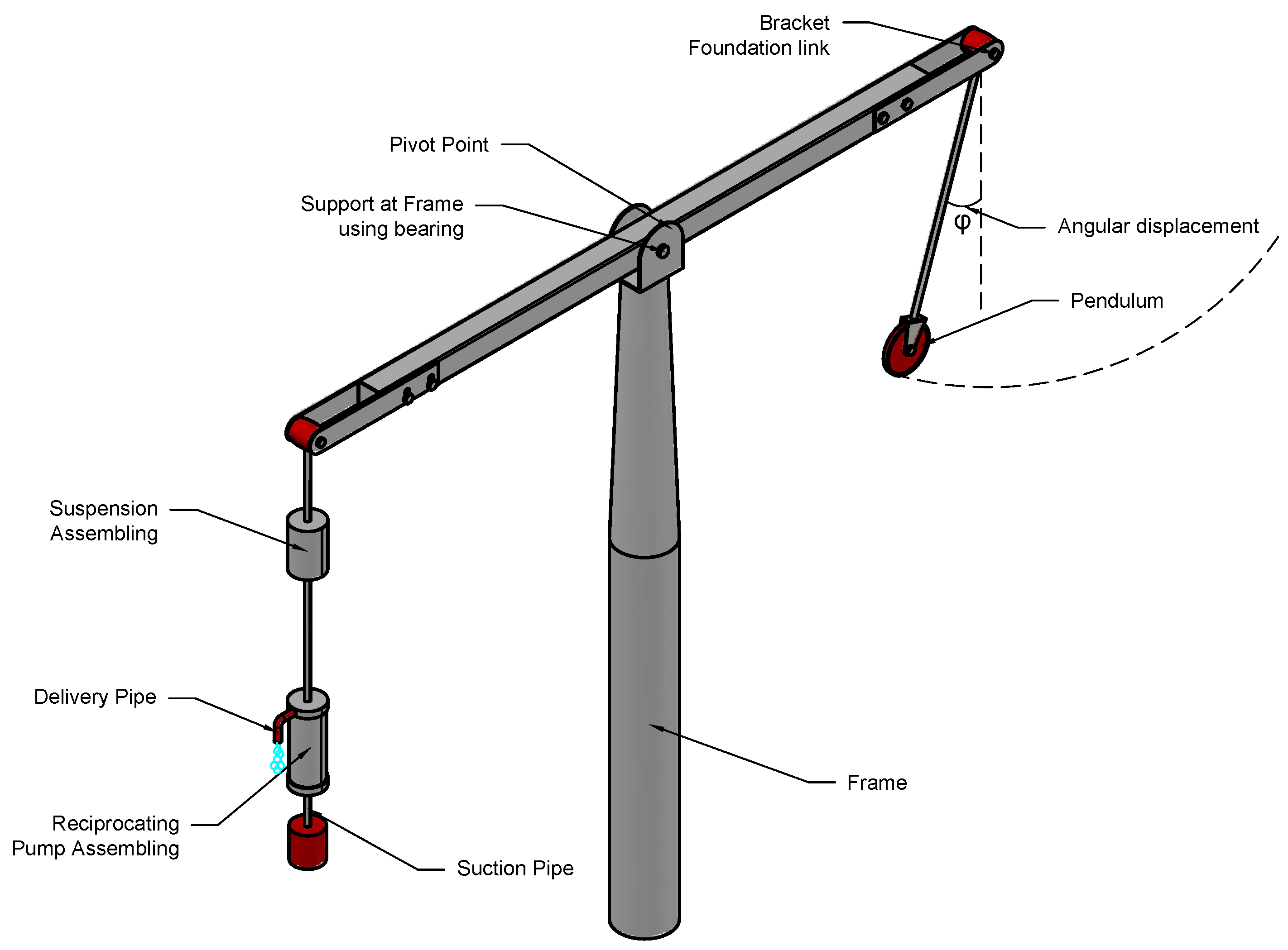
The proposed system comprises three main parts: the pendulum, the lever, and the reciprocating pump assembly containing the piston and the pushrod. Other parts include bracket foundation link, pivot point, frame, support at the frame, delivery pipe, and suction pipe. Figure 3 shows the three-dimensional physical model with the various parts of the system. The pendulum’s angular motion is transmitted into the to-and-from motion of the piston through the lever and the pushrod [2].

The system input is from the pendulum where an initial force is applied. The lever and the spring act as a transmitter that transmits the energy to the piston (system output), where the pumping of the liquid takes place.

2.2. Components of the System

We modify the existing pendulum water pump to achieve a maximum effect by using a vertically excited parametric pendulum with variable length instead of the conventional pendulum. Each component is briefly described below:

Frame: the rigid part serving as a support where the whole system assembly is mounted.

The parametric pendulum with variable length: Ref. [16], the required energy source for commencing the action of pumping by oscillating. (Detailed in Section 3.1, case II).

Bracket: a connection between the pendulum and lever and also between the lever and the piston.

Pivot point: also called the fulcrum, it is the part where the lever turns. It plays a central role in the lever system, and the lever’s power is supplied between the pivot point and the pendulum.

Bearing: to reduce rotational friction and support axial loads.

The rod: held up by double support bearing one on each side of the lever that forms the lever’s fulcrum. The coupling of the lever crested on the bearing lever rotates with the use of thrashing. A different support bearing is utilized at the pendulum’s bracket, allowing for the pendulum’s motion.

Delivery pipe: it connects the pump’s cylinder with the exit. The liquid is dispatched to the preferred exit point along this delivery pipe.

Suction pipe: it connects the origin of liquid to the reciprocating pump’s cylinder. This pipe sucks the liquid from the source to the cylinder.

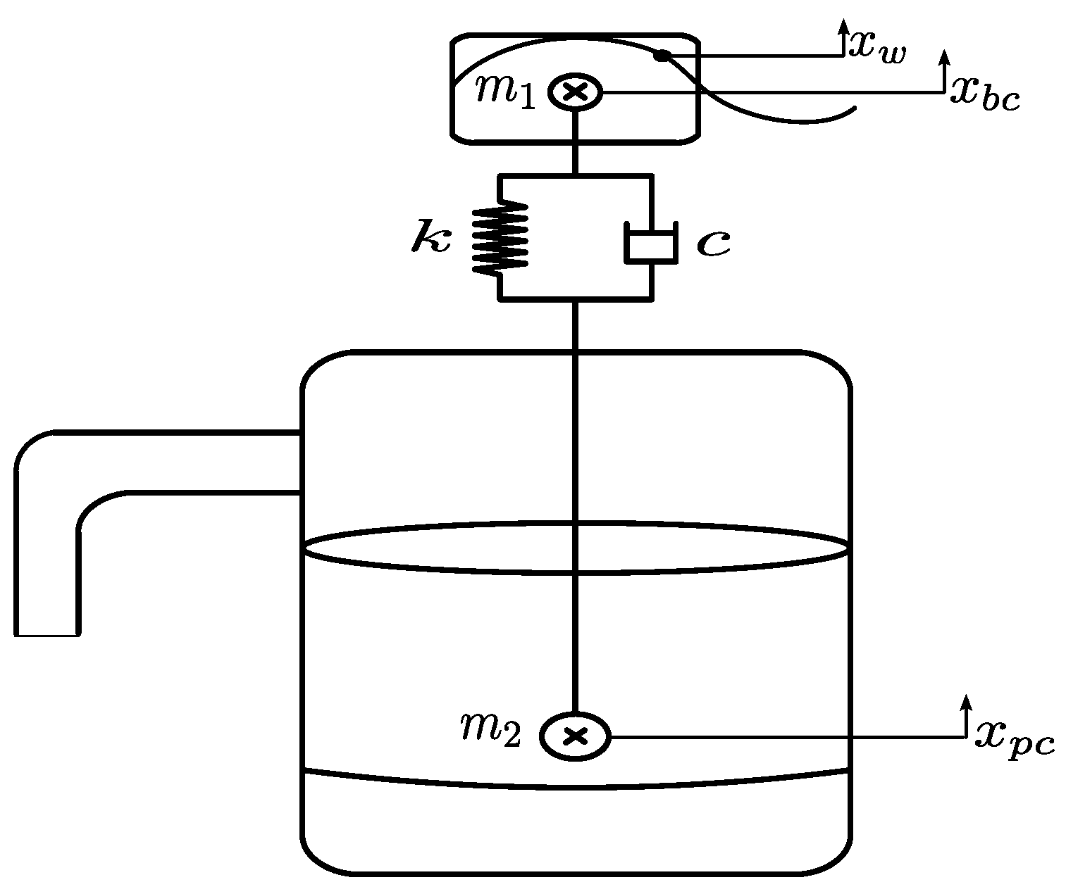
Reciprocating pump assembling: convert the mechanical energy into hydraulic energy by sucking the liquid into a cylinder. A piston is reciprocating, which uses thrust on the liquid and increases its hydraulic energy [17].

2.3. The Working Principle

The system free energy is based on the phenomenon of an oscillating pendulum-lever system. The pendulum pump’s purpose is the oscillation of the body pendulum controlled with a small pressure hand. Change of the inertial forces causes the fluctuation of the lever attached to the pump piston connected to a spring and a damper. The oscillations of the pendulum serve as the model’s input [18]. These oscillations bring about the swinging to and fro of the lever about its turning position; the lever is attached at one end to the pump’s rod and brings about the lever movement. For water to flow from the pump, the pendulum does not need to be balanced. Instead, the piston starts oscillating based on gravitational potential, and water begins to come out through the delivery pipe continuously. The pendulum is to be pushed occasionally in other to maintain the continuous flow of water. The pendulum water pump works efficiently with 90${}^{\circ }$ amplitude regardless of the pendulum’s size [6]. The foot valve opens at the piston’s upstroke, and suction brings water into the pump’s upper part (head) from the suction pump. The piston’s valve opens up and permits water to spout upward above the piston on the piston’s following downstroke. On the subsequent piston’s upstroke, water is propelled over the exit [19]. The system does not require fuel or electricity for its operation. Therefore, it is user-friendly and cannot cause global warming.

3. Mathematical Modeling

The complete system is made up of three parts: the pendulum, lever, and piston. These are modeled separately and connected through the bracket, where forces are transferred from one part to another. The motion of one makes the subsequent part move. As the pendulum is set to motion, it transfers the force to actuate the lever. The lever motion is imparted to the piston. The motion equation is established from Newton’s second law of motion, i.e., $F=ma$ since a force initiates the motion.

3.1. The Pendulum

Two cases are presented below in deriving the equations of motion of the pendulum. Case I follows the standard models using Newton’s second law of motion to derive the pendulum with constant length equations. The works existing in literature use this type of pendulum to act as the system inputs. In Case II of the present work, we used a vertically excited parametric pendulum with variable length as the system input. Hence, more frequent and faster oscillations can be achieved. In this case, the Euler–Lagrange equation is utilized to obtain the governing equations.

Case I: The energy needed for starting the pumping process is initiated by swinging the pendulum with minimum effort [20,21]. The pendulum model showing the free body diagram is shown in Figure 4, and its equation of motion is derived below. The force response does not transmit a moment around the position 0, where the rotation takes place. Therefore, the sum of the moments is 0 about the attachment point.

Summing all moments of forces, the following equation is found:

$$\sum M_t=I_0\ddot{\phi },$$

(3)

$$\sum M_t=-(m+m_b)glsin\phi -T_v+T_h,$$

(4)

where: $m_b$—pendulum’s bar mass (kg), m—the pendulum body mass (kg), l—length to the pivot of mass of the end weight (m), $T_v$—moment of viscous friction force (N·m), $T_h$—excitation moment (N·m), $\phi$—pendulum angular displacement (rad), $I_0$—mass moment of inertia (kg·m²), and g—acceleration due to gravity (m/s²).

Simplifications: (i) the pendulum mass is concentrated in the center point of the end mass; (ii) $sin\phi \approx \phi$, so we assume small angles of rotation in this case.

The mass moment of inertia $I_0$ is given as:

$$I_0\approx (m+m_b)l^2,$$

(5)

For a more accurate approach, we consider the body’s relative mass of the system to be situated at the system’s pivot of mass, which is:

$$l_g=\frac{\left(ml+0.5m_{b}l\right)}{\left(m+m_b\right)},$$

(6)

so the mass moment of inertia yields:

$$I_0=\frac{m_b{l}^2}{3}+m{l}^2.$$

(7)

The moment of viscous friction $T_v$$=b\dot{\phi }$, where b (N·s·m⁻¹) states the coefficient of viscous damping.

Equation (4) becomes:

$$-\left(m+m_b\right)g{l}_{g}sin\phi -b\dot{\phi }+T_h=I_0\ddot{\phi },$$

(8)

and at the assumed simplifications:

$$\ddot{\phi }+\frac{b}{I_0}\dot{\phi }+\frac{\left(m+m_b\right)g{l}_g\phi }{I_0}=T_h,$$

(9)

where: $T_h=$$f_{0}cos\omega t$, $f_0$—amplitude of forcing excitation (N·m).

The linearized method has the configuration of a typical unconstrained differential equation of the second-order. Complementing Equation (9) to a canonical form, one finds

$$\ddot{\phi }+2\zeta {\omega }_n\dot{\phi }+{\omega }_n^2\phi =T_h,$$

(10)

where ${\omega }_n$ is the excitation frequency (rad·s⁻¹), $\zeta$ is the damping coefficient (N·s·m⁻¹), $2\zeta {\omega }_n=\frac{b}{I_0}$, ${\omega }_n^2=\frac{\left(m+m_b\right)g{l}_g\phi }{I_0}$. Later, we will show how numerous variables of the system affect the independent response of the pendulum coupling. For the simplified pendulum having its mass concentrated at its end, we find:

$${\omega }_n\approx \sqrt{\frac{g}{l}}.$$

(11)

Case II: As shown in Figure 5, Lagrange’s equation is utilized to derive the governing equation of the vertically excited parametric pendulum with variable length [16] using the sine function as input for the angular position [16].

It is possible to remodel the overall length of the pendulum $l_{03}$ by readjusting the location of the telescopic bar, $l_{02}$. As the bar is recanted, the original length of the pendulum $l_{01}$ ($l_{03}=l_{01}$) is regained. The centre of rotation is stimulated vertically as a result of excised motion $I=I\left(t\right)$. Using the Euler–Lagrange equation in two degrees of freedom, the unconventional system is expressed in Equation (12)

$$\frac{d}{dt}\left(\frac{\partial L}{\partial \dot{q}}\right)-\frac{\partial L}{\partial q}+\frac{\partial D}{\partial \dot{q}}=0,$$

(12)

where: $\phi$(t)—angular displacement defined from the downward inclination point, $E_k$—kinetic energy equation of the system, $E_p$—potential energy, and D—dissipative energy of the system:

$$\begin{array}{cc}\hfill E_k=& \frac{1}{2}m\left({\left({\dot{x}}_e\left(t\right)sin\phi \left(t\right)+cos\phi \left(t\right)\left(l_{01}+l_{02}+x_e\right)\dot{\phi }\left(t\right)\right)}^2+\right.\hfill \\ \hfill & \left.{\left(-f_0\omega sin\left(\omega t\right)+{\dot{x}}_e\left(t\right)cos\phi \left(t\right)-sin\phi \left(t\right)\left(l_{01}+l_{02}+x_e\right)\dot{\phi }\left(t\right)\right)}^2\right),\hfill \end{array}$$

(13)

$$E_p=\frac{1}{2}k{x}_e^2\left(t\right)-gm\left(f_{0}cos\left(\omega t\right)+cos\phi \left(t\right)\left(l_{01}+l_{02}+x_e\left(t\right)\right)\right),$$

(14)

$$D=\frac{1}{2}{c}_p{\dot{\phi }}^2\left(t\right).$$

(15)

where: m—the mass of the pendulum body (a bob), k—spring stiffness, $c_p$—viscous damping coefficient of the pendulum. Putting Equations (13)–(15) into Equation (12) and carrying out the analogous derivatives, the equation of motion is obtained as presented in Equations (16) and (17):

$$\begin{array}{cc}\hfill \ddot{\phi }=& \left(\frac{1}{m\left(l_{01}+l_{02}+x_e\right)\left(l_{01}+l_{02}+x_e\right)}\right)\left(-m\left(l_{01}+l_{02}\right)\left(g+f_0{\omega }^{2}cos\left(\omega t\right)\right)sin\phi \left(t\right)-\right.\hfill \\ \hfill & \left.c_p\dot{\phi }\left(t\right)-m{x}_e\left(t\right)\left(g+f_0{\omega }^{2}cos\left(\omega t\right)sin\phi \left(t\right)\right)-m\left(l_{01}+l_{02}+x_e\left(t\right)\right)\left(2{\dot{x}}_e\left(t\right)\dot{\phi }\left(t\right)\right)\right),\hfill \end{array}$$

(16)

$$\begin{array}{cc}\hfill {\ddot{x}}_e\left(t\right)=& gcos\phi \left(t\right)+f_0{\omega }^{2}cos\left(\omega t\right)cos\phi \left(t\right)-\frac{k{x}_e\left(t\right)}{m}-\frac{c{\dot{x}}_e\left(t\right)}{m}+l_{01}{\dot{\phi }}^2\left(t\right)+\hfill \\ & l_{02}{\dot{\phi }}^2\left(t\right)+x_e\left(t\right){\dot{\phi }}^2\left(t\right).\hfill \end{array}$$

(17)

The motion considered here is the enforce motion existing as a sinusoidal wave of the conformation $I\left(t\right)=f_{0}cos\left(\omega t\right)$, where $f_0$ is the excitation amplitude.

The above equation regains the established governing equation of the vertical parametric pendulum when $l_{03}$ is varied due to the extension $x_e$. It is assumed that an external force causes the excitation. Thus, we assumed the almost ideal case where an external force could partially compensate for dissipation of mechanical energy through a frictional contact from the human effort [16,22].

3.2. The Lever

The lever amplifies the pendulum force and transmits the force to the piston through the bracket foundation link. To understand the lever model fully, we start with a simple model, as can be seen in Figure 6, which shows the lever with the pivot in the middle of the lever or center of gravity (CG), assuming that the CG is at the middle of the lever, that is, $l_1$ is equal to $l_2$. Figure 7 represents the lever component showing the pendulum’s connection and then to the piston through two different bracket foundation links, respectively. From Newton’s second law, the equation of motion of the lever is obtained, where $\phi$ is denoted as the input for the lever model, which is the output from the pendulum model.

Analyzing Figure 6, one writes: $x_1=l_{1}sin\phi$, $x_2=l_{2}sin\phi$ and $\frac{x_1}{x_2}=\frac{l_1}{l_2}=L$. In addition, $\frac{v_1}{v_2}=\frac{l_1}{l_2}$ states a ratio of lever arms: where $l_1$—distance from $f_1$ and position p, $l_2$—distance from $f_2$ and position p, $x_1$ and $x_2$ are the displacements at both ends of the lever. With small-angle approximation and the motion at the lever end to be purely translational in ‘x’ direction, the relationship between the forces and displacements is carried out by summing the torques T around the pivot point (about fulcrum), i.e.,

$$\sum _{ccw}{T}_{ccw}-\sum _{cw}{T}_{cw}=0,$$

(18)

where the subscript $ccw$—counter-clockwise direction, and $cw$—clockwise direction. With the relations: $f_1{l}_1-f_2{l}_2=0$ (balance of momentums), $f_1{l}_1=f_2{l}_2$ or $\frac{f_1}{f_2}=\frac{l_2}{l_1}=\frac{1}{L}$ (conservation of power in levers, see [23]); $f_1$ and $f_2$ (N) are the forces on both ends of the lever.

It can be noted that the force relationship with the velocity relationship is given as $\frac{v_1}{v_2}=\frac{l_1}{l_2}=L$.

Therefore,

$$\frac{v_1}{v_2}.\frac{f_1}{f_2}=\frac{l_1}{l_2}.\frac{l_2}{l_1}=1,$$

(19)

where we find that the power is preserved if $v_1{f}_1=v_2{f}_2$, so it is the same on both sides of the lever.

In Figure 7, one observes that the lever arms are unequal; one side will experience a higher force and velocity than the other side. We assume some definitions $F_k=-kx$, $F_c=-cx$, $F=m\ddot{x}$, and $l_3=\frac{1}{3}{l}_2$, which is the distance from $CG$ to p, k stiffness of the stiffness (N·m⁻¹), and c—viscous damping coefficient (N·s·m⁻¹).

Using Newton’s second law, the lever governing equation is obtained as follows:

$$m_l\ddot{x}{l}_3+c\dot{x}{l}_2+kx{l}_2=f_1\left(t\right)l_1,$$

(20)

where $m_l$—is the total mass of the lever, x—is the displacement of the lever. $f_1\left(t\right)=sin\phi$.

3.3. Piston Model

According to [20,24], piston has a reverse effect on the lever, and it damps oscillations of the pump. Damping of the lever motion causes damping of the pendulum, but the force damping the pendulum is less than the work of force that dampens the lever. Figure 8 shows a schematic diagram of the piston. An analysis leads to the equations of motion, as it is shown below.

We introduce the following denotations for the masses (kg): $m_1$—buoy mass, $m_2$—piston model mass (total), $m_3$—mass of the rod, $m_4$—mass of the piston, $m_5$—mass of the pumped fluid, together with the two relations $m_2=m_3+m_4+m_5$ in the upstroke and $m_2=m_3+m_4$ in the down stream. Therefore, the mass $m_2$ changes in time t as it moves upward and downward. In addition, the mass $m_2$ is different in the upstroke due to the pumping processes of the fluid. Ref. [25] delivers a mathematical representation of the dynamical motion of the piston given in a state-space representation as it follows:

$$\dot{q}=Aq+f,\mathrm{for}q\left(0\right) = q_0.$$

(21)

The state vector is presented as:

$$q={\left. [x_{bc}{\dot{x}}_{bc}{x}_{pc}{\dot{x}}_{pc}{p}_{ur}{p}_{lr}\right]}^T,$$

(22)

where: $x_{bc}$—position of the buoy’s center of mass (m), ${\dot{x}}_{bc}$—buoy velocity (m·s⁻¹), $x_{pc}$—position of the piston center (m), ${\dot{x}}_{pc}$—piston velocity (m·s⁻¹), $p_{ur}$—upper reservoir pressure (Pa), $p_{lr}$—lower reservoir pressure (Pa).

The governing equations are given in Equations (23) and (24):

$$m_1{\ddot{x}}_{bc}+c\left({\dot{x}}_{bc}-{\dot{x}}_{pc}\right) + k\left(x_{bc}-x_{pc}-l_R\right) =F_{bc}-m_{1}g,$$

(23)

where: $l_R$—length of the rod (m), $F_{bc}$—force of the buoy’s center of mass (N).

We get the second-order differential equation of dynamics of the piston:

$$m_2{\ddot{x}}_{pc}+c\left({\dot{x}}_{pc}-{\dot{x}}_{bc}\right) + k\left(x_{pc}-x_{bc}-l_R\right) = {-A}_c\left(p_{ur}-p_{lr}\right)-m_{2}g-F_f,$$

(24)

where:

$$x_{bc}=\frac{L_r+0.5H_b-\left(m_1+m_4+\rho A_c\left(L_c+H_u\right)\right)}{\left(S_b{\rho }_{sw}-\frac{H_w}{2}\right)},$$

(25)

$$x_{pc}=\frac{0.5H_b-\left(m_1+m_4+\rho A_c\left(L_c+H_u\right)\right)}{\left(S_b{\rho }_{sw}-\frac{H_w}{2}\right)}.$$

(26)

Continuing, the pumping force is found in the following form:

$$F_p=-A_c{p}_{lr}+\rho \left(l_c{+L}_u\right)A_{ur}\left({\ddot{z}}_p+g\right)+\rho A_c{\dot{z}}_p^2,$$

(27)

where area of the piston $A_c=\pi {R_p}^2$ (m²), $z_p$—piston displacement about a zero mean, $A_{ur}$—area of the upper reservoir (m²), $F_f$—initial approximation of the friction in the contact between the piston and the cylinder given as $-B{\dot{x}}_{pc}$, $B=\frac{\mu }{S_p}2\pi R_p{H}_p$—cylinder damping coefficient (N·s·m⁻¹), $S_p$—separation of piston and cylinder (m), $R_p$—radius of the piston (m), and $H_p$—height of the piston (m).

The amount of water pumped by the piston in every upstroke is the water in the cylinder, and the water inside the upper reservoir. Because of this, the fluid mass has to be modified as follows:

$$m_5=\rho \left(l_c+\frac{p_{ur}}{\rho g}\right)A_c,$$

(28)

where: $\rho$—density of the fluid (kg·m⁻³), g—gravitational acceleration (m·s⁻²), and $l_c$—length of the cylinder (m).

The buoyancy force depending on the buoy $X_{bc}$ and the position of the wave $x_w$ is given in the form [25]:

$$F_{bc}= \left(x_w-x_{bc}+\frac{1}{2}{H}_b\right)S_b{\rho }_{sw}g,$$

(29)

where: $H_b$—height of the buoy (m), $S_b$—surface of the buoy, ${\rho }_{sw}$—reservoir fluid density (kg·m⁻³) and $x_w$—definition of wave used for the simulation is given:

$$x_w=L_r+\frac{H_w}{2}sin\left(\frac{2\pi }{T_w}t-\frac{\pi }{2}\right),$$

(30)

where: $H_w$—wave height (m), $T_w$—wave period (s).

4. Numerical Results and Discussion

The numerical solutions of the system governing equations are solved using the Runge–Kutta method with adaptive step-size, with a simulation time step size of $0.003$ s for case I and $0.005$ s for case II. The initial condition for the pendulum angle $\phi \left(0\right)$ is $0.5\pi$ radians for both case I and case II, with a time scale of 30 s and 50 s for the case I and case II, respectively.

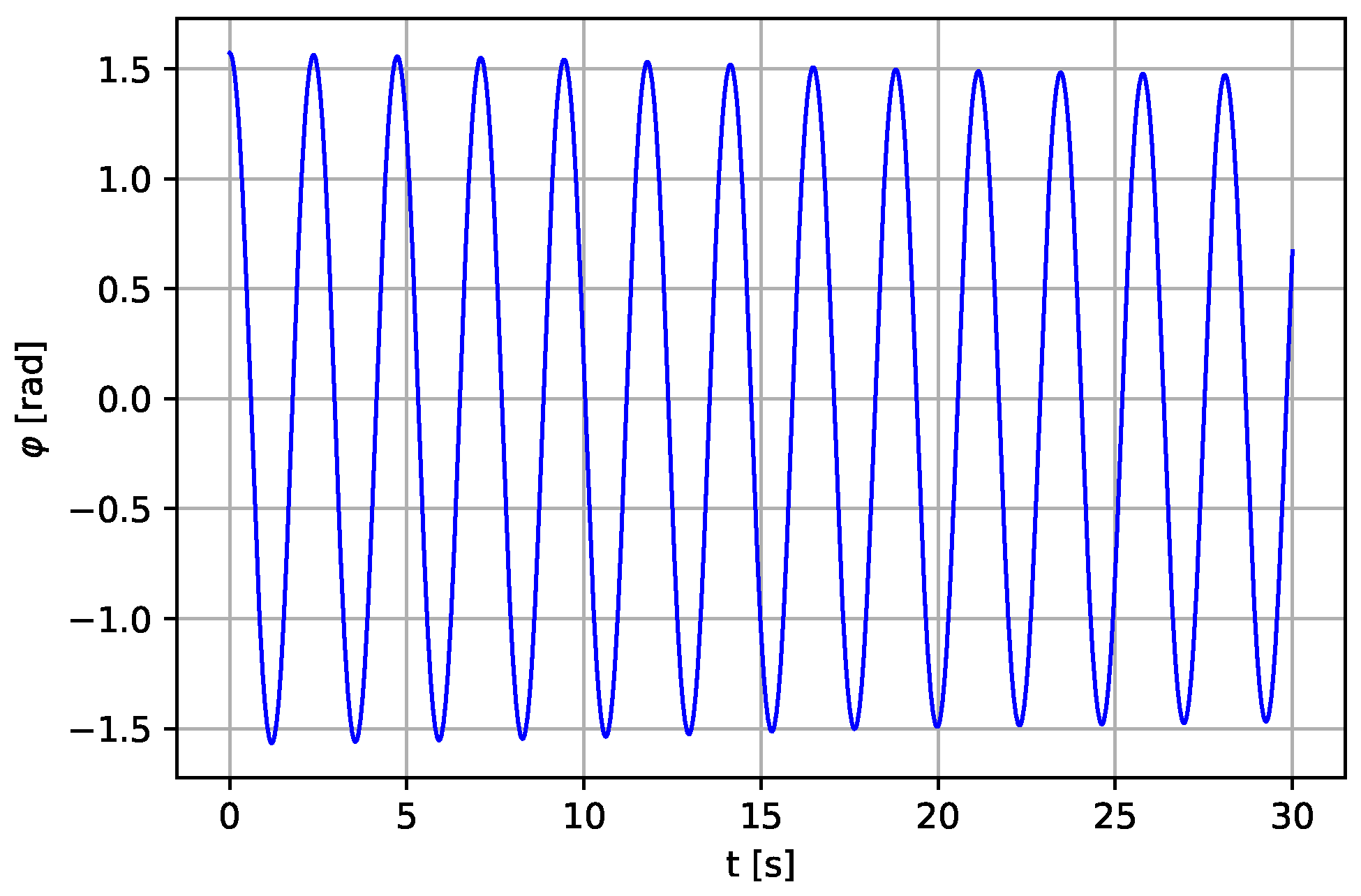
Case I: Water pump pendulum with constant length. We start with the pendulum displacement, then the lever displacement, and finish at the piston’s displacement. Finally, various parameters that determine the pendulum pump’s output discharge are analyzed, and the numerical results are presented in Figure 9, Figure 10 and Figure 11 for the pendulum, lever, and piston displacement, respectively. Parameters analysis includes the pendulum’s mass, angle of suspension, and the pendulum’s length. Therefore, we present only the results with the parameters that show good system responses.

For the pendulum displacement, the computations are performed using the below stated parameter values: $l=0.5$ m, $M=0.38$ kg, $m=0.095$ kg, $f_0=0.005$ N, $\omega =5$ rad·s⁻¹, $g=9.81$ m·s⁻², $b=0.003$ N·s·m⁻¹. The period of rotational motion depends on the length of the pendulum. The length is varied at a point in time until the desired periods are obtained. As shown in Figure 9, amplitude of the total energy decreases with time due to damped oscillations. Therefore, the pendulum has to be push occasionally for a continuous fluid flow.

Simulation of the lever displacement is shown in Figure 10, using the following parameter values: $m_l=2.0$ kg $c=1.0$ N·s·m⁻¹, $k=5.0$ N·m⁻¹, $l_1=0.4$ m, $l_2=0.6$ m, $l_3=\frac{1}{3}{l}_2$, $f_1\left(t\right)=sin\phi$, where $\phi$—the pendulum angular displacement (rad) is the pendulum system input. The results show that the total energy gradually decreases with time.

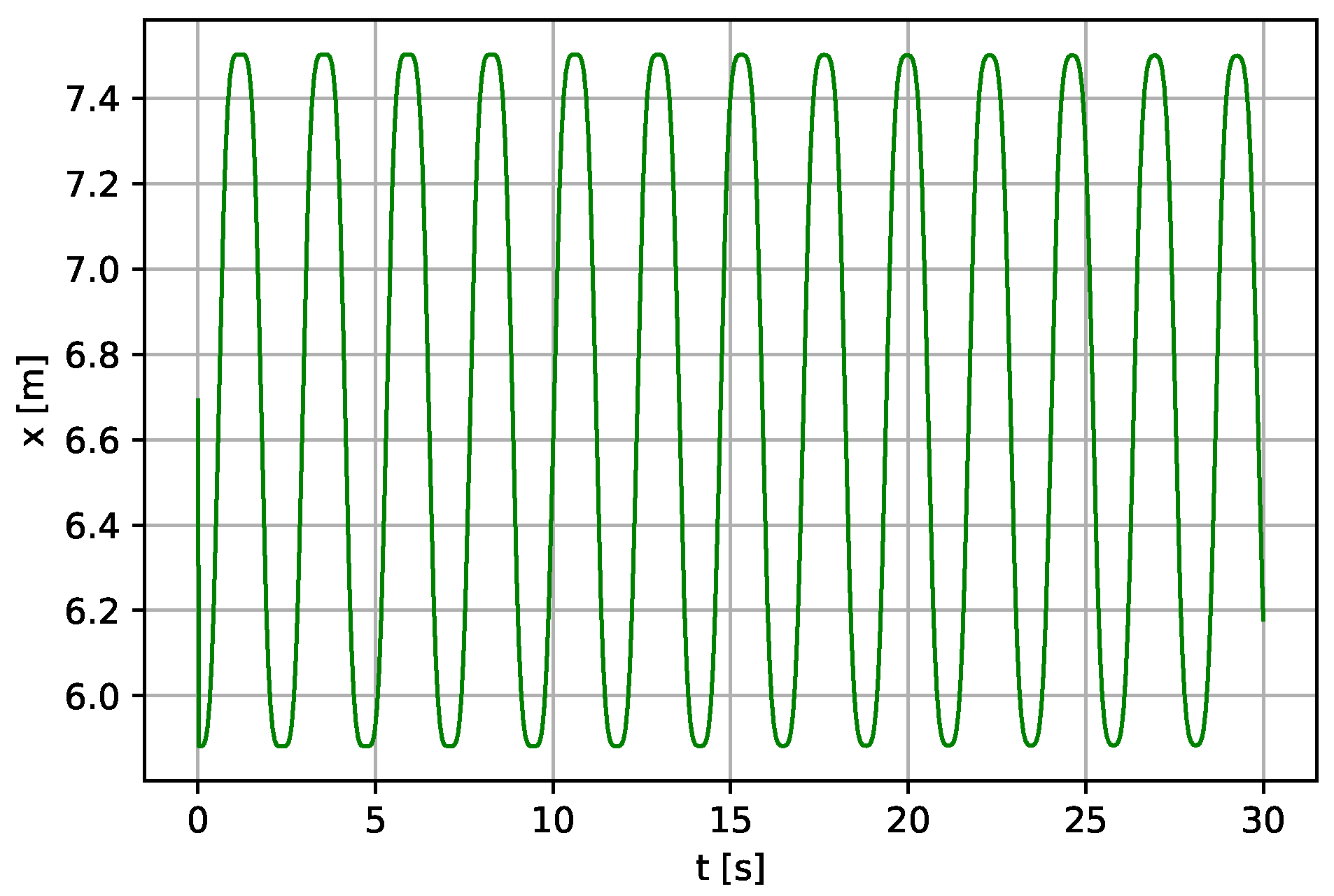
An analysis of the piston is presented. Some studies of fluid mechanics are also included in the piston analysis for optimal pump performance. The linear displacement of the piston is shown in Figure 11 with the values of the parameters as $m_1=10$ kg, $g=9.81$ m·s⁻², $c=1.0$ N·s·m⁻¹, $k=50.0$ N·m⁻¹, $l_R=4$ m, $g=9.81$ m·s⁻²,$B=1.25915$ N·s·m⁻¹, $m_2=6.0242$ kg, $\rho =1000$ kg·m⁻², ${\rho }_{sw}=1030$ kg·m⁻²$A_{ur}=4$ m², $A_{lr}=4$ m², $s_b=2$ m, $H_b=2$ m, $T_w=10$ s, $H_w=4$ m, $L_c=10$ m, $z_p=0$ m, $H_p=2$ m, $L_r=2$ m $z_p=0$ m, $R_p=0.05$ m². The same values for the spring constant, k, and the viscous damping constant, c, was used because of the same connection. It can be observed that the response of the piston is similar to the lever displacement. However, the displacement is not as much as that of the lever because of higher piston mass and other considered factors, overall pump parameters, and fluid analysis.

The analysis for different lengths is carried out for a deeper understanding of the relation between pendulum length and output of the system, which was not addressed in [5]. Changing the right-hand side pendulum length alone, i.e., without changing initial parameters of other parts, affects performance of the whole system. Therefore, the efficiency of the pumping depends on the length of the right-hand side pendulum. As can be seen in Figure 12, Figure 13 and Figure 14, the system becomes more stable, but with a reduced number of oscillation periods for the whole system when the parameter value l is changed from $0.5$ to $1.2$ m.

The simulation results shown in Figure 9, Figure 10, Figure 11, Figure 12, Figure 13 and Figure 14 have been compared with the result delivered by [5]. It has proved that our model follows a more realistic trend because it includes friction and the effect of excitation force on the response of the investigated system. Furthermore, the presented system in case I is more stable than one in [5], as shown in Figure 1, Figure 2 and Figure 12, Figure 13 and Figure 14. The obtained results clearly show how the pendulum’s length plays a critical role in the overall system stability.

In addition, further analysis of Case I of the pendulum model is carried out by increasing the viscous damping with other parameters left unchanged. When the viscous damping b is increased to $0.3$ N·s·m⁻¹ with the same length $l=1.2$ m, the time response of the system decreases and vanishes within a few seconds, as shown in Figure 15, Figure 16 and Figure 17. Providing some technical recommendations, the value of b should be minimum for the system to be more stable and oscillate for a more extended period. Therefore, the value of the pendulum length, l, and the viscous damping, b, are to be selected with care as they have more effect on the system performance.

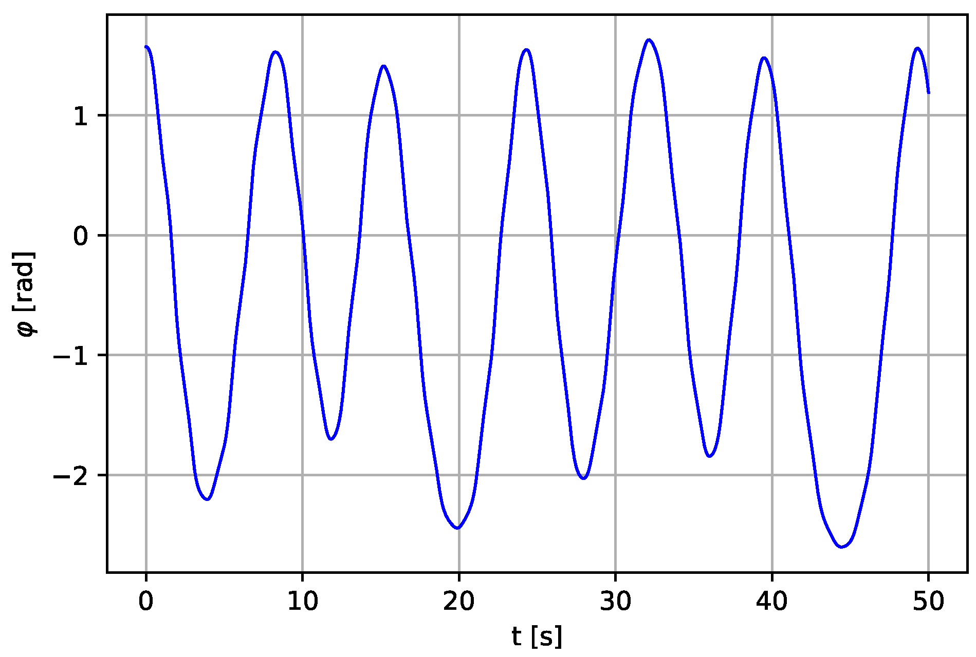
Case II: Water pump pendulum with a vertically excited parametric pendulum with variable length [16] is used instead of the conventional pendulum. 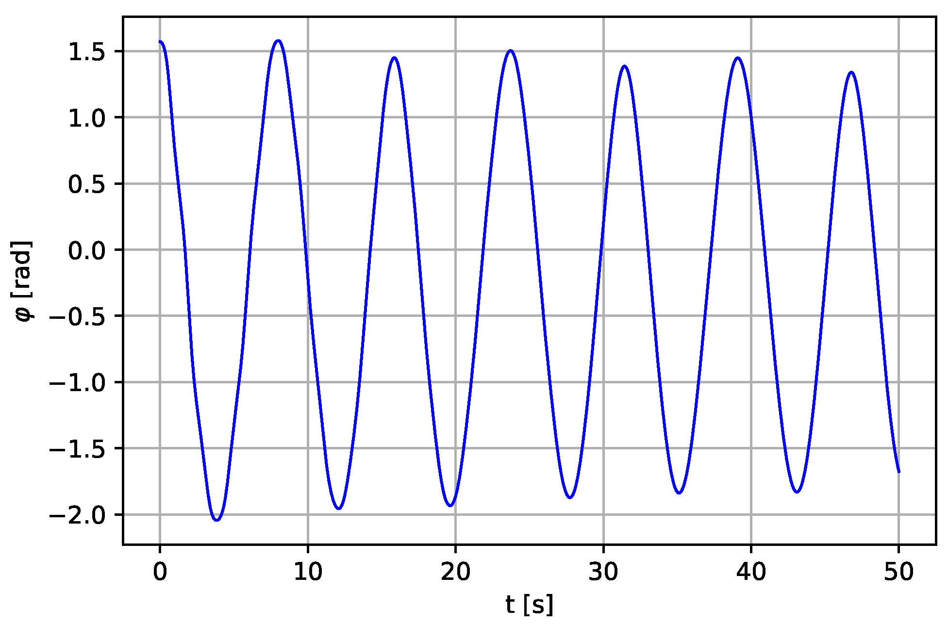Figure 18, Figure 19 and Figure 20 show the simulation results for the whole system when this type of pendulum with variable length is used with the following parameter values: $l_{01}=l_{02}=4$ m, $m=5$ kg, $x_e=1.5$ m, $f_0=10$ N, $\omega =0.5$ rad·s⁻¹, $g=9.81$ m·s⁻², $c_p=0.1$ N·s·m⁻¹. The parameters’ values of the lever and the piston remain unchanged. With $c_p=1$ N·s·m⁻¹ and $\omega =0.4$ rad·s⁻¹, Figure 21, Figure 22 and Figure 23 are obtained, which shows more stable oscillation of the variable-length pendulum with more stability of the lever and the piston model as a result of the effect of increasing damping.

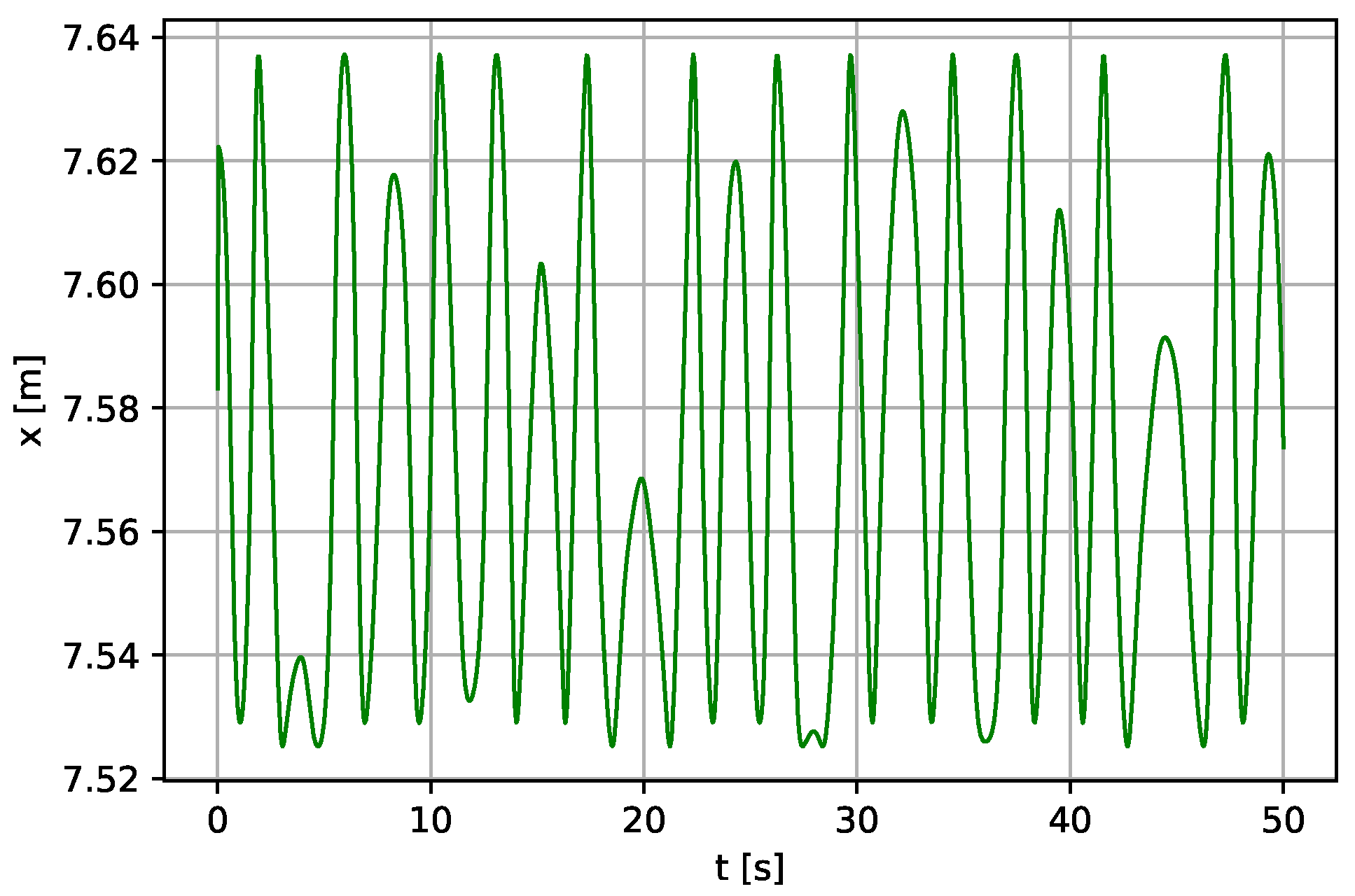
Figure 18, Figure 19, Figure 20, Figure 21, Figure 22 and Figure 23 show the time histories of the pendulum, lever, and piston, respectively. Some irregularity and quasi-periodicity are reported, and the behavior does not settle even after 50 s of simulation time. The pattern of recurrence does not lend to precise measurement. However, the oscillations can occur regularly when a regular external forcing forces them. In other words, the quasi-periodicity behavior can be compensated when a regular external forcing is applied to the system.

5. Conclusions

A nonlinear model of a pendulum is used to power the model of the piston through the lever. The system’s dynamic response is analyzed, and the presented results show the system’s effectiveness after a series of simulations at various parameter values. The numerical results show a good response of the scenario through the power transient from the pendulum to the piston. In addition, the system’s response depends on the length of the pendulum that can be manipulated to achieve better performance. The presented results also show that the system can transfer energy with little human effort to do heavy work since the piston’s mass is much bigger than the combined mass of the pendulum and the lever. A novelty is presented where a vertically excited pendulum with variable length is used instead of the conventional pendulum with constant length. In the proposed model, the system response shows a quasi-periodicity behavior and does not settle even after 50 s of simulation time. However, the quasi-periodicity behavior can be compensated when a regular external forcing is applied to the system. No control algorithm is included since the aim is to operate a system in rural and urban areas without electricity. However, the system can be constructed to include a control algorithm and transformed into a mechatronics system for any laboratories and industrial uses. Synchronization of the pendulum pump and the human body could be considered a problem of biomechanics. Lastly, further dynamical analysis can be performed to investigate the system’s behavior more, and more studies on fluid mechanics will add value to the overall system operation.

References

1. Government of Canada. Water in Developing Countries. 2021. Available online: https://www.international.gc.ca/world-monde/issues_development-enjeux_developpement/environmental_protection-protection_environnement/water-eau.aspx?lang=eng (accessed on 31 March 2021).
2. Bain, R.E.S.; Gundry, S.W.; Wright, J.A.; Yang, H.; S., P.; Bartram, J.K. Accounting for water quality in monitoring access to safe drinking-water as part of the Millennium Development Goals: Lessons from five countries. Bull. World Health Organ. 2012, 90, 228–235. [Google Scholar] [CrossRef] [Green Version]
3. Nikhade, G.R.; Patil, R.; Bansal, S.P. Two-stage oscillator mechanism for operating a reciprocating pump. Asian J. Sci. Technol. 2013, 4, 37–41. [Google Scholar]
4. Cavalheiro, M. Pendulum pump. Natl. J. Energy 2001, 1, 156. [Google Scholar]
5. Memon, M.A.; Nizamani, A.R.; Hussain, A.; Rajper, M.L.; Kumar, B.; Ali, Z. Mathematical Modeling of Pendulum Hand Pump. Stud. Res. Pap. Conf. 2015, 2, 245–249. [Google Scholar]
6. Vigithra, R.; Ajith, V.; JayaKrishna, B.R.; Ajithkumar, R.; Dinesh, S. Design and Fabrication of Pendulum Hand Water Pump. J. Innov. Res. Dev. 2016, 1, 71–75. [Google Scholar]
7. Okoronkwo, C.A.; Ezurike, B.O.; Uche, R.; Igbokwe, J.O.; Oguoma, O.N. Design of a hand water pump using a quick-return crank mechanism. Afr. J. Sci. Technol. Innov. Dev. 2016, 8, 292–298. [Google Scholar] [CrossRef]
8. Shelar, P.B.; Kambale, A.D.; Patil, A.N.; Khandare, R.M.; Sachane, A.H.; Gavali, S.S. Design and Development of Pendulum Operated Water Pump. Int. Res. J. Eng. Technol. (IRJET) 2018, 5, 1387–1389. [Google Scholar]
9. Apparao, D.; Sagar, Y. Design and Development of Hand Water Pump with a Pendulum. Int. J. Eng. Manag. Res. 2017, 5, 357–361. [Google Scholar]
10. Manoj, C.; Manjunath, T.N.; Raghavendra, G.; Ramakrishna, G.P. Design and Fabrication of Pendulum Operated Pump. Int. J. Sci. Adv. Res. Technol. 2018, 4, 611–614. [Google Scholar]
11. Rajendra, T.N.; Rajendra, S.N.; Dattatraya, K.D.; Satish, A.L.; Patwari, A. Pendulum operated hand pump. Int. Res. J. Eng. Technol. (IRJET) 2019, 6, 2740–2743. [Google Scholar]
12. Śmiechowicz, W.; Loup, T.; Olejnik, P. Lyapunov Exponents of Early Stage Dynamics of Parametric Mutations of a Rigid Pendulum with Harmonic Excitation. Math. Comput. Appl. 2019, 24, 90. [Google Scholar] [CrossRef] [Green Version]
13. Pietrzak, P.; Ogińska, M.; Krasuski, T.; Figueiredo, K.; Olejnik, P. Near the resonance behavior of a periodically forced partially dissipative three-degrees-of-freedom mechanical system. Lat. Am. J. Sci. Struct. 2018, 15. [Google Scholar] [CrossRef]
14. Olejnik, P.; Fečkan, M.; Awrejcewicz, J. Analytical and numerical study on a parametric pendulum with the step-wave modulation of length and forcing. Int. J. Struct. Stab. Dyn. 2018, 19, 1941006. [Google Scholar] [CrossRef]
15. Krasilnikov, P.; Gurina, T.; Svetlova, V. Bifurcation study of a chaotic model variable-length pendulum on a vibrating base. Int. J. Non-Linear Mech. 2018, 105, 88–98. [Google Scholar] [CrossRef]
16. Reguera, F.; Dotti, F.E.; Machado, S.P. Rotation control of a parametrically excited pendulum by adjusting its length. Mech. Res. Commun. 2016, 72, 74–80. [Google Scholar] [CrossRef]
17. Reciprocating Pump—Components, Working and Uses. Available online: https://theconstructor.org/practical-guide/reciprocating-pump-components-working-uses/2914/ (accessed on 15 April 2021).
18. Rath, K.C.; Samanta, P.K.; Kanhara, D.K. A brief study on Pendulum based Pump. Int. J. Mod. Trends Eng. Res. (IJMTER) 2016, 3, 57–62. [Google Scholar]
19. Gowrishankar, K.; Gobinath, M.; Gani, R. Single Acting Piston Pump Using Oscillating Motion. Int. J. Res. Mech. Eng. Technol. 2015, 5, 27–29. [Google Scholar]
20. Anand, A.; Jhakal, D.; Sharma, R.; Deshbhratar, R. Fabrication of Pendulum Pump. Int. J. Sci. Eng. Res. 2017, 8, 68–70. [Google Scholar]
21. Singh, R.; Kumar, V. Swing up and Stabilization of Rotary Inverted Pendulum using TS Fuzzy. Int. J. Sci. Res. Eng. Technol. 2014, 2, 753–759. [Google Scholar]
22. Cliffort, M.J. Bishop, S.R. Rotating periodic orbit of the parametrically excited pendulum. Phys. Lett. A 1995, 201, 191–196. [Google Scholar] [CrossRef]
23. Schlaudt, O. Hölder, Mach, and the Law of the Lever: A Case of Well-founded Non-controversy. Philos. Sci. 2013, 17, 93–116. [Google Scholar] [CrossRef]
24. Jong, K.L.; Jun, K.J.; Jang-Bom, C.; Jin-Woo, L. Mathematical modeling of reciprocating pump. J. Mech. Sci. Technol. 2015, 29, 3141–3151. [Google Scholar]
25. Galván, G.B. Nonlinear Control Design for Wave Energy Converter. Master’s Thesis, University of Groningen, Groningen, The Netherlands, 2014; pp. 1–76. [Google Scholar]
Figure 1. Angular displacement of the Pendulum in Equation (1).
Energies 14 08064 g001
Figure 2. Linear displacement of the Piston in Equation (2).
Energies 14 08064 g002
Figure 3. Configuration of the three-dimensional model of the investigated system.
Energies 14 08064 g003
Figure 4. The pendulum free body diagram.
Energies 14 08064 g004
Figure 5. Schematic diagram of the vertical parametric pendulum with variable-length.
Energies 14 08064 g005
Figure 6. Schematic diagram of the lever device.
Energies 14 08064 g006
Figure 7. Schematic diagram of the lever device and connecting components like spring and damper.
Energies 14 08064 g007
Figure 8. Schematic diagram of the piston.
Energies 14 08064 g008
Figure 9. Angular displacement φ ( t ) of the pendulum for l = 0.5 m, b = 0.003 N·s·m−1.
Energies 14 08064 g009
Figure 10. Linear displacement x ( t ) of the lever for l = 0.5 m, b = 0.003 N·s·m−1.
Energies 14 08064 g010
Figure 11. Linear displacement x p c of the piston l = 0.5 m, b = 0.003 N·s·m−1.
Energies 14 08064 g011
Figure 12. Linear displacement φ ( t ) of the pendulum (continued) for l = 1.2 m, b = 0.003 N·s·m−1.
Energies 14 08064 g012
Figure 13. Linear displacement x ( t ) of the lever (continued) for l = 1.2 m, b = 0.003 N·s·m−1.
Energies 14 08064 g013
Figure 14. Linear displacement x p c of the piston (continued) for b = 0.003 N·s·m−1.
Energies 14 08064 g014
Figure 15. Linear displacement φ ( t ) of the pendulum (continued) for l = 1.2 m, b = 0.3 N·s·m−1.
Energies 14 08064 g015
Figure 16. Linear displacement x ( t ) of the lever (continued) for l = 1.2 m, b = 0.3 N·s·m−1.
Energies 14 08064 g016
Figure 17. Linear displacement x p c of the piston (continued) for l = 1.2 m, b = 0.3 N·s·m−1.
Energies 14 08064 g017
Figure 18. Angular displacement φ ( t ) of the pendulum (Case II—a variable length concept of the pendulum pump) for c p = 0.1 N·s·m−1, ω = 0.5 rad·s−1.
Energies 14 08064 g018
Figure 19. Linear displacement x ( t ) of the lever (Case II—a variable length concept of the pendulum pump) for c p = 0.1 N·s·m−1, ω = 0.5 rad·s−1.
Energies 14 08064 g019
Figure 20. Linear displacement x p c ( t ) of the piston (Case II—a variable length concept of the pendulum pump) for c p = 0.1 N·s·m−1, ω = 0.5 rad·s−1.
Energies 14 08064 g020
Figure 21. Angular displacement φ ( t ) of the pendulum (Case II—a variable length concept of the pendulum pump) for c p = 1 N·s·m−1, ω = 0.4 rad·s−1.
Energies 14 08064 g021
Figure 22. Linear displacement x ( t ) of the lever (Case II—a variable length concept of the pendulum pump) for c p = 1 N·s·m−1, ω = 0.4 rad·s−1.
Energies 14 08064 g022
Figure 23. Linear displacement x p c ( t ) of the piston (Case II—a variable length concept of the pendulum pump) for c p = 1 N·s·m−1, ω = 0.4 rad·s−1.
Energies 14 08064 g023
Publisher’s Note: MDPI stays neutral with regard to jurisdictional claims in published maps and institutional affiliations.