On the Relationship between Oil and Exchange Rates of Oil-Exporting and Oil-Importing Countries: From the Great Recession Period to the COVID-19 Era

Abstract

This paper is dedicated to studying and modeling the interdependence between the oil returns and exchange-rate movements of oil-exporting and oil-importing countries. Globally, twelve countries/regions are investigated, representing more than 60% and 67% of all oil exports and imports. The sample period encompasses economic and natural events like the Great Recession period (2007–2009) and the COVID-19 pandemic. We use the dynamic conditional correlation mixed-data sampling (DCC-MIDAS) model, with the aim of investigating the interdependencies expressed by the long-run correlation, which is a smoother (but always daily observed) version of the (daily) time-varying correlation. Focusing on the advent of the COVID-19 pandemic in 2020, the long-run correlations of the oil-exporting countries (Saudia Arabia, Russia, Iraq, Canada, United States, United Arab Emirates, and Nigeria) and (lagged) WTI crude oil returns strongly increase. For a subset of these countries (that is, Saudia Arabia, Iraq, United States, United Arab Emirates, and Nigeria), the (lagged) correlations turn out to be positive, while for Canada and Russia they remain negative as before the advent of the pandemic. In addition, the oil-importing countries and regions under investigation (Europe, China, India, Japan, and South Korea) experience a similar pattern: before the COVID-19 pandemic, the (lagged) correlations were negative for China, India, and South Korea. After the COVID-19 pandemic, the correlations of these latter countries increased.

1. Introduction

During the last fifteen years, many events affecting oil prices have occurred. According to the United States Energy Information Administration (EIA), there were four main economic and natural events that happened from 2007 onwards and affected crude oil prices. These events are as follows: the global financial collapse (2008, second quarter—Q2), the consequent (2009, Q1) oil production cut from the Organization of the Petroleum Exporting Countries (OPEC), the OPEC decision to keep the production quota unchanged (2015, Q2), and, finally, the oil reduction demand caused by the advent of the COVID-19 pandemic. The literature has largely investigated oil price reactions in the aftermath of these events. For instance, ref. [1] examined the volatility of the Brent, Dubai, and West Texas Intermediate (WTI) crude oil returns by means of the logistic smooth transition autoregressive-generalised autoregressive conditional heteroskedasticity (GARCH) model, focusing on the impact of the COVID-19 pandemic. Ref. [2] analyzed the spillovers between crude oil and the United States (USA) and Chinese stock markets as well as the gold futures market, through a Markov-switching vector autoregressive model, during the pandemic. Ref. [3] used the heterogeneous autoregressive realized volatility model with an additional covariate related to infectious diseases to estimate the WTI volatility. A decent number of papers have researched the macroeconomic effects of oil shocks on major economies such as the United States [4], the euro area [5], and several other developed economies [6]. Other studies have focused on the impact of oil shocks on the external accounts of oil exporters and major oil importers [7] or the current account of the United States [8].

According to numerous studies and observations, it became clear that “a fluctuating real exchange rate impairs on economic growth” [9]. Following [10], the volatility of oil prices negatively affects non-oil sectors and formation of capital. Paper [11] proved that income per capita is damaged by oil price fluctuations. This topic has been on the agenda for many years already and scientists have attempted to find the connection or to prove that no connection exists between oil prices and currency exchange rates. For instance, ref. [12] provided empirical support for the theoretically stated link between exchange rates and oil prices. Ref. [13] examined the dynamics of this relationship in the short-term and long-term; the work of [14] is dedicated to the explaining and forecasting of one variable with another (oil prices with currency exchange rates and vice versa) with the use of econometric methods. Ref. [15] takes a closer look at the financial aspects of the relationship between oil price fluctuations and exchange rates by building a multifactor model. Ref. [16] studied the causal relationship between studied variables and investigated the bidirectional nonlinear relation between oil and exchange rate, and between oil and stock price. Ref. [17] considered asymmetric models to study the interdependence between oil prices and exchange rate co-movements. A closer look at the relationship between Russian ruble exchange rate fluctuations and oil price dynamics was taken in [18] and a regression model was built as empirical proof for theoretical assumptions. Ref. [19] found that oil prices are among the main drivers of the real effective exchange rate movements of three oil-exporting countries (Azerbaijan, Kazakhstan, and Russia).

If the literature has largely investigated, both from univariate and multivariate perspectives, the relationships between oil prices and other stock markets, there is still some on-going debate on the connections between oil and exchange rates. For instance, ref. [20] found that, using weekly data, an increase in oil prices leads to an exchange rate depreciation and vice versa. The co-movements between the oil prices and exchange rates have also been recently reviewed by [21]. In their contribution, the authors claim that the exchange rates and oil prices are interconnected over the long-run. Taking as a starting point what was found in [21], this paper aims at investigating the long-run correlation among the exchange rates of the largest oil-exporting and oil-importing countries and regions and the WTI crude oil returns, with a particular emphasis on the periods following the previously mentioned EIA-signaled events. The analysis is conducted by means of the dynamic conditional correlation (DCC, [22]) model, in the version proposed by [23], which is the specification with the mixed-data sampling (MIDAS, [24]) term in the correlation part. From this point of view, the current work could be seen as a continuation of [25]. However, if the latter work considers three exporting and three importing countries, we use a larger panel of countries, covering approximately 60% and 67% of all exporting and importing oil shares, respectively. Moreover, [25] analyzed the dynamic relationship between stock markets and crude oil returns, while we focus on exchange rates and oil returns. Finally, from a methodological point of view, we use the DCC-MIDAS model with the exponential GARCH [26] as a model for the univariate specification, while [25] adopted a DCC-GJR specification. Resorting to the DCC-MIDAS model to investigate the long-term correlation is not new in the literature, generally for the superior forecasting ability with respect to the standard DCC specification (see [27,28], among others). Recently, [29] investigated the long-term correlation between two crude oil markets (WTI and Brent) and four stock markets (US, Europe, Japan, and United Kingdom). The DCC-MIDAS model has also been applied to investigate the relationships between oil returns and exchange rates by [30,31]. In more detail, ref. [30] focused on the WTI and Brent markets related to seven exchange rates, using a sample period spanning from 2000 to 2017. Ref. [31], using the period from 1994 to 2015, investigated the long-run correlation between WTI returns and four exchange rates. Our contribution differs from the previous two for at least two reasons. First, we cover an updated period (up to June 2021, also including the COVID-19 pandemic) and larger oil-exporting and oil-importing countries/regions. Second, we investigate not only the contemporaneous correlation between the previous mentioned variables, but also the lagged correlations. In the lagged long-run correlation, we model the effect that lagged oil returns may have on today’s exchange rates, in the spirit of [32], which found that an increase in the oil price leads to appreciation of the US dollar.

The rest of the paper is structured as follows. Section 2 is devoted to a description of the methods used to perform the further analysis. Section 3 presents the empirical analysis. Section 4 summarizes key points of the paper and provides directions for further research.

2. Methodology

Let ${\mathit{r}}_t={\left[r_{t,1},\cdots ,r_{t,n}\right]}^{\prime }$ be the vector of n daily log-returns observed at time t, with $t=1,\cdots ,T$. According to the DCC literature, we assume that:

$$\begin{array}{ccc}\hfill {\mathit{r}}_t& \sim & MVN(0,H_t)\hfill \end{array}$$

(1)

$$\begin{array}{ccc}\hfill H_t& =& D_t{R}_t{D}_t,\hfill \end{array}$$

(2)

where $MVN$ stands for the multivariate normal distribution; $H_t$ represents the $(n\times n)$ conditional covariance matrix; $D_{i,t}$ is the diagonal matrix including the conditional standard deviations ${\sigma }_{t,1},\cdots ,{\sigma }_{t,n}$ on the main diagonal; and $R_t$ is the correlation matrix, which is obtained as:

$$\begin{array}{ccc}\hfill R_t& =& E_{t-1}\left[{\mathsf{\xi }}_t{\mathsf{\xi }}_t^{\prime }\right]\hfill \end{array}$$

(3)

$$\begin{array}{ccc}\hfill {\mathsf{\xi }}_t& =& D_t^{-1}{\mathit{r}}_t.\hfill \end{array}$$

(4)

In Equation (3), $E_{t-1}\left[·\right]$ is the conditional expectation for t made at time $t-1$. Hence, ${\mathsf{\xi }}_t$ represents the standardized residuals obtained from the univariate volatility models. Under the Equations (1)–(4), we have that:

$$\begin{array}{ccc}\hfill {\mathit{r}}_t& =& H_t^{1/2}{\mathsf{\xi }}_t\hfill \end{array}$$

(5)

$$\begin{array}{ccc}\hfill {\mathsf{\xi }}_t& \stackrel{iid}{\sim }& MVN(0,I_n),\hfill \end{array}$$

(6)

where $I_n$ denotes the $n\times n$ dimensional identity matrix.

In the DCC class of models, the estimation phase is split into two steps. In the first step, the univariate models are separately estimated in order to define the matrix $D_t$. In the second step, the models for the correlation matrix $R_t$ are estimated. Let ${\mathrm{\Theta }}_v$ and ${\mathrm{\Theta }}_c$ be the parameter spaces of the volatility and correlation models, respectively, with $\mathrm{\Theta }=\left\{{\mathrm{\Theta }}_v,{\mathrm{\Theta }}_c\right\}$. In line with [22], the full log-likelihood function, labeled as $\mathcal{L}\left(\mathrm{\Theta }\right)$, is:

$$\begin{array}{ccc}\hfill \mathcal{L}\left(\mathrm{\Theta }\right)& =& \mathcal{L}\left({\mathrm{\Theta }}_v\right)+\mathcal{L}\left({\mathrm{\Theta }}_c\right)\hfill \\ & =& -{\displaystyle \sum _{t=1}^T}\left[nlog\left(2\pi \right)+2log|D_t|+{\mathit{r}}_t^{\prime }{D}_t^{-2}{\mathit{r}}_t\right]\hfill \end{array}$$

(7)

$$\begin{array}{ccc}& & -{\displaystyle \sum _{t=1}^T}\left[log|R_t|+{\mathsf{\xi }}_t^{\prime }{R}_t^{-1}{\mathsf{\xi }}_t+{\mathsf{\xi }}_t^{\prime }{\mathsf{\xi }}_t\right].\hfill \end{array}$$

(8)

The univariate specification used in this work is the EGARCH(1,1) model, which is, for an asset j:

$$ln{\sigma }_{t,j}^2=\omega +\alpha \left(|{\mathsf{\xi }}_{t-1,j}|-E\left(|{\mathsf{\xi }}_{t-1,j}|\right)\right)+\gamma {\mathsf{\xi }}_{t-1,j}+\beta ln{\sigma }_{t-1,j}^2,\mathrm{with}j=1,\cdots ,n.$$

(9)

The dynamics of the correlation matrix $R_t$ follows the DCC-MIDAS model. Formally:

$$\begin{array}{ccc}\hfill R_t& =& {\left(\mathit{diag}\left(Q_t\right)\right)}^{-1/2}{Q}_t{\left(\mathit{diag}\left(Q_t\right)\right)}^{-1/2}\hfill \end{array}$$

(10)

$$\begin{array}{ccc}\hfill Q_t& =& (1-a-b){\overline{R}}_t\left(w\right)+a\left({\mathsf{\xi }}_{t-1}{\mathsf{\xi }}_{t-1}^{\prime }\right)+b{Q}_{t-1}\hfill \end{array}$$

(11)

where a and b are scalars and ${\overline{R}}_t\left(w\right)$ is the long-run correlation, defined as:

$${\overline{R}}_t\left(w\right)=\sum _{k=1}^{K_c}{{\Phi }}_k\left(w\right)\odot C_{t-k},$$

(12)

with ${{\Phi }}_k\left(w\right)={\varphi }_k\left(w\right)\iota {\iota }^{\prime }$ denoting the weights associated to each lagged realization of the matrix $C_k$, ⊙ the Hadamard product, $\iota$ an $n\times 1$ vector of ones and ${\varphi }_k\left(w\right)$ a proper weighting function. In this work, we opt for the beta function, defined as:

$${\varphi }_k\left(w\right)=\frac{{(k/K_c)}^{w_1-1}{(1-k/K_c)}^{w_2-1}}{{\displaystyle \sum _{l=1}^{K_c}}{(l/K_c)}^{w_1-1}{(1-l/K_c)}^{w_2-1}}.$$

(13)

When $w_1=1$ and $w_2\ge 1$ in Equation (13), more emphasis is attributed to the most recent observations. In Equation (12), the matrix $C_k$ is:

$$C_t={\left(\begin{array}{ccc}{v}_{t,1}& 0& 0\\ ⋮& \ddots & 0\\ 0& \cdots & v_{t,n}\end{array}\right)}^{-1/2}\sum _{m=t-N_c}^t{\mathsf{\xi }}_m{\mathsf{\xi }}_m^{\prime }{\left(\begin{array}{ccc}{v}_{t,1}& 0& 0\\ ⋮& \ddots & 0\\ 0& \cdots & v_{t,n}\end{array}\right)}^{-1/2},$$

(14)

with

$$v_{t,j}=\sum _{m=t-N_c}^t{\mathsf{\xi }}_{m,j}^2,\forall j=1,\cdots ,n.$$

(15)

Hence, the long-run correlation ${\overline{R}}_t\left(w\right)$ at time t is a one-sided filter of the last $K_c$ realizations of the matrix $C_t$, which in turn depends on the last $N_c$ standardized squared returns ${\mathsf{\xi }}_{t,j}^2$. The larger $N_C$ and $K_c$ are, the smoother the long-run correlation is.

Once we have estimated the time-varying correlations, we build around them the confidence intervals, following the procedure also used by [33] (alternatively, other procedures have also been proposed; see, for instance, ref. [34]). Let ${\rho }_t$ be the correlation between two assets at time t (for ease of notation, we have suppressed here the indexes of the two assets). The 95% confidence intervals for ${\rho }_t$ make use of Fisher’s z-transformation of such correlation coefficient:

$$z_t=0.5log\left(\frac{1+{\rho }_t}{1-{\rho }_t}\right),\forall t=1,\cdots ,T.$$

(16)

Then, letting $tanh$ be the hyperbolic tangent function, the 95% confidence intervals are obtained as:

$$\left[tanh\left(z_t-\frac{1.96}{\sqrt{T-3}}\right);tanh\left(z_t+\frac{1.96}{\sqrt{T-3}}\right)\right],\forall t=1,\cdots ,T.$$

(17)

3. Empirical Analysis

We focus our attention on the top-seven oil-exporting and top-five oil-importing countries/regions. According to the OPEC archive (in particular, we have considered Tables 5.2 and 5.6 reported at https://asb.opec.org/data/ASB_Data.php (accessed on 24 August 2021), https://asb.opec.org/data/ASB_Data.php (accessed on 24 August 2021)), the top-seven exporting countries are Saudi Arabia, Russia, Iraq, Canada, United States, United Arab Emirates, and Nigeria. In 2019, these countries accounted for approximately 60% of all oil exports. The top-five oil importing countries/regions in 2019 were Europe, China, India, Japan, and South Korea (we have excluded from the oil-importing countries the United States, because it was already present in the list of oil-exporting ones). These chosen countries/regions imported about 67% of the world’s oil production. All the data were collected from the Yahoo Finance site. Data processing was performed in R, using the dccmidas [35] package.

Table 1. Mechanical properties of the materials.

	Currency	Min.	Max.	Mean	SD	Skew.	Kurt.
WTI crude oil EUR	−0.077	0.077	0.000	0.023	−0.122	1.785
Oil-exporting countries
Saudi Arabia	EUR/SAR	−0.063	0.034	−0.000	0.007	−0.108	4.134
Russia	EUR/RUB	−0.077	0.077	0.000	0.013	0.238	6.123
Iraq	EUR/IQD	−0.070	0.077	−0.000	0.007	0.295	13.210
Canada	EUR/CAD	−0.039	0.034	0.000	0.006	−0.023	2.808
United States	EUR/USD	−0.077	0.077	−0.000	0.007	−0.215	26.867
United Arab Emirates	EUR/AED	−0.069	0.044	−0.000	0.008	0.054	3.347
Nigeria	EUR/NGN	−0.077	0.077	0.000	0.010	0.375	14.872
Oil-importing countries
Europe	USD/EUR	−0.077	0.077	0.000	0.007	0.235	26.867
China	EUR/CNY	−0.077	0.077	−0.000	0.008	−0.008	14.033
India	EUR/INR	−0.045	0.041	0.000	0.007	0.042	2.388
Japan	EUR/JPY	−0.058	0.077	−0.000	0.008	−0.284	8.315
South Korea	EUR/KRW	−0.077	0.077	0.000	0.009	−0.019	7.300

reports some summary statistics for the returns series under investigation, while Figure 1 and Figure 2 illustrate their patterns. From Table 1 it can be noted that almost all returns distributions have heavy tails, since kurtosis is greater than 3 (leptokurtic distributions). Only WTI crude oil, EUR/CAD, and EUR/INR exchange rates are platykurtic. Such a situation of non-normality of returns is a very common case for assets traded on the stock market. By analyzing Figure 1 and Figure 2, we can state that neither oil-exporting nor oil-importing countries’ exchange rates share the same pattern. However, as concerns oil-exporting countries, we can clearly set apart United States, Saudi Arabia, Iraq, and United Arab Emirates as countries with very similar patterns of exchange rate dynamics, which is obviously explained by the fixed exchange rate regime of the latter three. Exchange rates for Nigeria and Russia experience overall upward dynamics, whereas the Canadian dollar is gradually strengthening against the euro. As concerns oil-importing countries, their exchange rate dynamics are very different from each other. Nevertheless, we can split these exchange rates into overall upward dynamics (USD/EUR, EUR/INR), downward dynamics (EUR/KRW, EUR/CNY), and flat market (EUR/JPY).

For modeling the dynamics of correlations we obtain from the closing prices of the series under investigation the close-to-close daily log-returns. We focus first on the contemporaneous correlations and then on the lagged correlations, as done by [25], for instance. In the lagged correlations, the vector ${\mathit{r}}_t$ has the oil variable expressed as $r_{t-1}$. In other words, we evaluate the impact of yesterday’s oil variation on today’s exchange rates. First we evaluate parameters of EGARCH(1,1) models for oil-exporting (see

Table 2. Oil-exporting countries: univariate models.

	Estimate	Std. Error	t Value	Pr($>\left|\mathbf{t}\right|$)	Sig.
	Saudi Arabia
$\omega$	−0.134	0.004	−32.351	0.000	***
$\alpha$	−0.061	0.011	−5.455	0.000	***
$\beta$	0.986	0.000	3974.267	0.000	***
$\gamma$	0.103	0.006	18.424	0.000	***
	Russia
$\omega$	−0.227	0.095	−2.389	0.017	**
$\alpha$	−0.006	0.028	−0.206	0.837
$\beta$	0.972	0.009	103.250	0.000	***
$\gamma$	0.226	0.023	9.803	0.000	***
	Iraq
$\omega$	−0.290	0.011	−25.602	0.000	***
$\alpha$	0.019	0.027	0.700	0.484
$\beta$	0.969	0.002	589.088	0.000	***
$\gamma$	0.194	0.030	6.407	0.000	***
	Canada
$\omega$	−0.122	0.004	−31.660	0.000	***
$\alpha$	0.019	0.011	1.778	0.075	*
$\beta$	0.988	0.000	2934.942	0.000	***
$\gamma$	0.113	0.004	26.754	0.000	***
	United States
$\omega$	−0.017	0.010	−1.651	0.099	*
$\alpha$	−0.018	0.014	−1.307	0.191
$\beta$	0.998	0.001	1225.251	0.000	***
$\gamma$	0.145	0.011	13.611	0.000	***
	United Arab Emirates
$\omega$	−1.037	0.981	−1.058	0.290
$\alpha$	−0.102	0.035	−2.886	0.004	***
$\beta$	0.891	0.102	8.743	0.000	***
$\gamma$	0.308	0.115	2.683	0.007	***
	Nigeria
$\omega$	−0.119	0.151	−0.789	0.430
$\alpha$	−0.008	0.021	−0.396	0.692
$\beta$	0.985	0.015	67.631	0.000	***
$\gamma$	0.202	0.057	3.534	0.000	***
	WTI crude oil
$\omega$	−0.110	0.008	−14.430	0.000	***
$\alpha$	−0.074	0.008	−8.771	0.000	***
$\beta$	0.985	0.001	984.155	0.000	***
$\gamma$	0.110	0.014	7.605	0.000	***

Notes: The table reports the estimates of the EGARCH models. Column Std. Error reports the quasi-maximum likelihood standard errors. Sample period: January 2007 to June 2021. Number of observations: 3563. *, **, and *** represent the significance at levels 10%, 5%, and 1%, respectively.

) and oil-importing countries (see

Table 3. Oil-importing countries: univariate models.

	Estimate	Std. Error	t Value	Pr($>\left|\mathbf{t}\right|$)	Sig.
	Europe
$\omega$	−0.017	0.010	−1.657	0.098	*
$\alpha$	0.018	0.014	1.312	0.190
$\beta$	0.998	0.001	1222.118	0.000	***
$\gamma$	0.145	0.011	13.567	0.000	***
	China
$\omega$	−1.207	1.110	−1.088	0.277
$\alpha$	−0.063	0.034	−1.848	0.065	*
$\beta$	0.875	0.113	7.716	0.000	***
$\gamma$	0.379	0.122	3.100	0.002	***
	India
$\omega$	−0.262	0.274	−0.956	0.339
$\alpha$	0.001	0.025	0.033	0.974
$\beta$	0.973	0.026	37.231	0.000	***
$\gamma$	0.158	0.272	0.583	0.560
	Japan
$\omega$	−0.172	0.022	−7.974	0.000	***
$\alpha$	−0.057	0.013	−4.338	0.000	***
$\beta$	0.982	0.002	468.840	0.000	***
$\gamma$	0.162	0.035	4.630	0.000	***
	South Korea
$\omega$	−0.360	0.086	−4.168	0.000	***
$\alpha$	−0.047	0.018	−2.616	0.009	***
$\beta$	0.960	0.009	107.259	0.000	***
$\gamma$	0.272	0.026	10.439	0.000	***
	WTI crude oil
$\omega$	−0.110	0.008	−14.430	0.000	***
$\alpha$	−0.074	0.008	−8.771	0.000	***
$\beta$	0.985	0.001	984.155	0.000	***
$\gamma$	0.110	0.014	7.605	0.000	***

Notes: The table reports the estimates of the EGARCH models. Column Std. Error reports the quasi-maximum likelihood standard errors. Sample period: January 2007 to June 2021. Number of observations: 3563. *, **, and *** represent the significance at levels $10\%,5\%,1\%$, respectively.

).

As one can see from Table 2, $\omega$ coefficients prove to be significant at least at the level of 10%. The only two exceptions are UAE and Nigeria, for which we stick to the hypothesis that $ln{\sigma }_{t,j}^2$ has no drift component. Parameters $\beta$ and $\gamma$, which are responsible for inertial and autoregressive components, respectively, are always positive and highly significant for all presented models. Positive values of $\gamma$ coefficients indicate the situation in which positive returns seem to increase volatility on the next step and negative ones seem to decrease it. Coefficients $\alpha$, which incorporate the magnitude of ${\mathsf{\xi }}_{t,j}$, are significant only for Saudi Arabia, UAE, and WTI crude oil.

Next, from Table 3, one can see that all EGARCH coefficients are 1% significant for Japan and South Korea, whereas only $\beta$ and $\gamma$ are 1% significant for Europe and China, which indicates presence of inertial and autoregressive components, respectively. Again, positive values of $\gamma$ coefficients state that positive returns tend to increase volatility and vice versa. Finally, only the inertial component is significant for India.

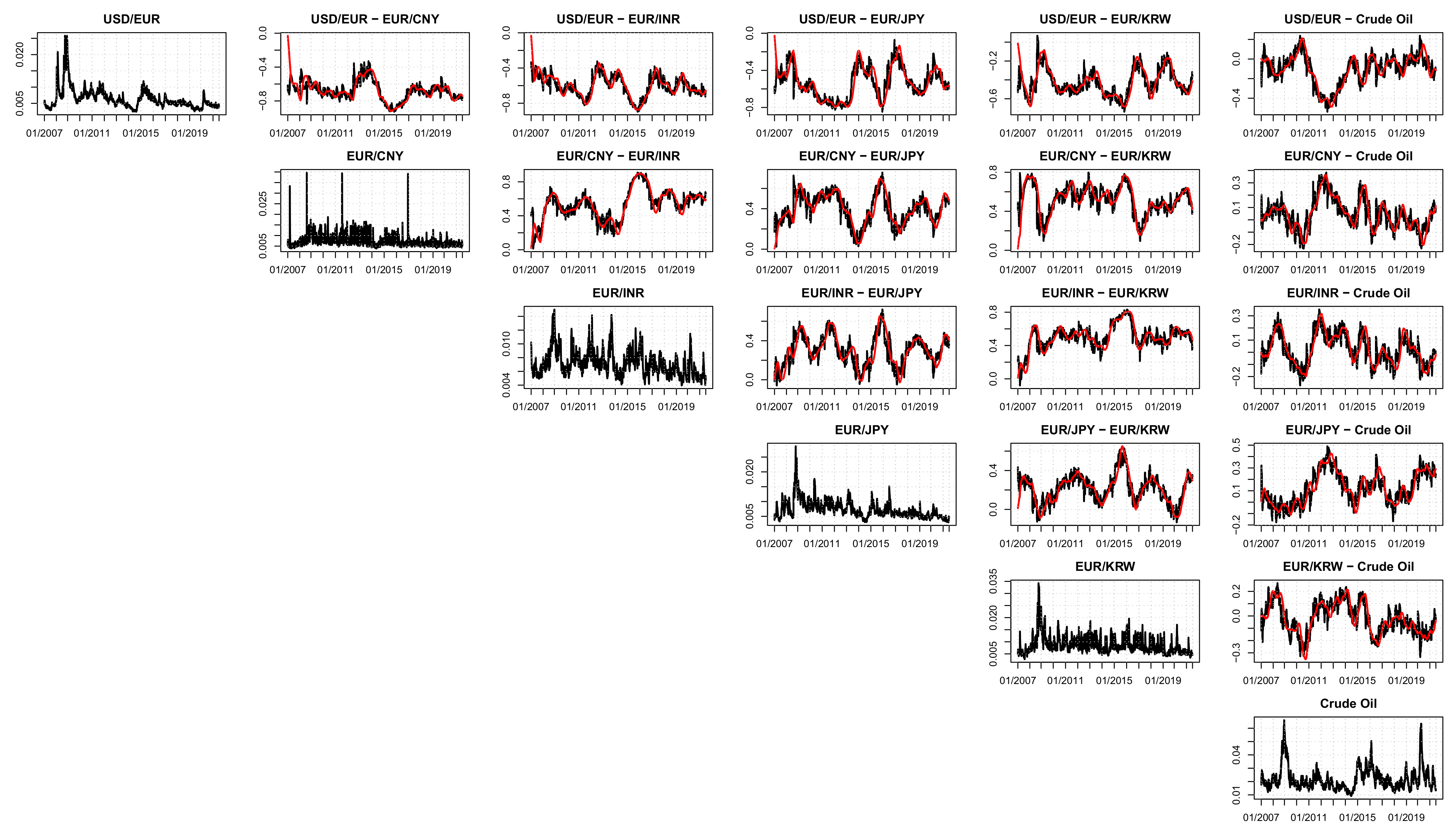
3.1. Contemporaneous Correlations

In Figure 3 and Figure 4 we present the results of the DCC-EGARCH-MIDAS model for the volatilities and contemporaneous correlations of exchange rates of oil-exporting countries and WTI crude oil log-returns. By analyzing these two figures we can say that most of the time correlations are negative, which implies that a rise in oil prices draws the currency exchange rate down and vice versa. This makes perfect economic sense, since oil-based income forms a decent share of international reserves in an oil-exporting country. Since the state budget of such a country is partly formed by taxes that oil-exporting companies pay, if the oil price goes down, revenues also go down, consequently driving down taxes, which makes the country lack a significant share of the state budget, which determines the decrease in supply of international currencies on the domestic market. Consequently this process weakens the national currency given that its supply is relatively stable. From Figure 4 we see that there was only one period of time right after the Great Recession that corresponded to positive correlations for nearly all considered exchange rates except for Canada and Russia.

As concerns oil-importing countries (see Figure 5 and Figure 6), we see that they are also mostly negative except for Europe, which is just the reverse of the United States correlation dynamics. All analyzed countries experience positive correlations of national currency exchange rates and WTI crude oil log-returns right after the Great Recession. Just like for oil-exporting countries, the obtained correlations reveal a very similar pattern, only for oil-importing countries do the analyzed correlations have an even stronger connection to each other.

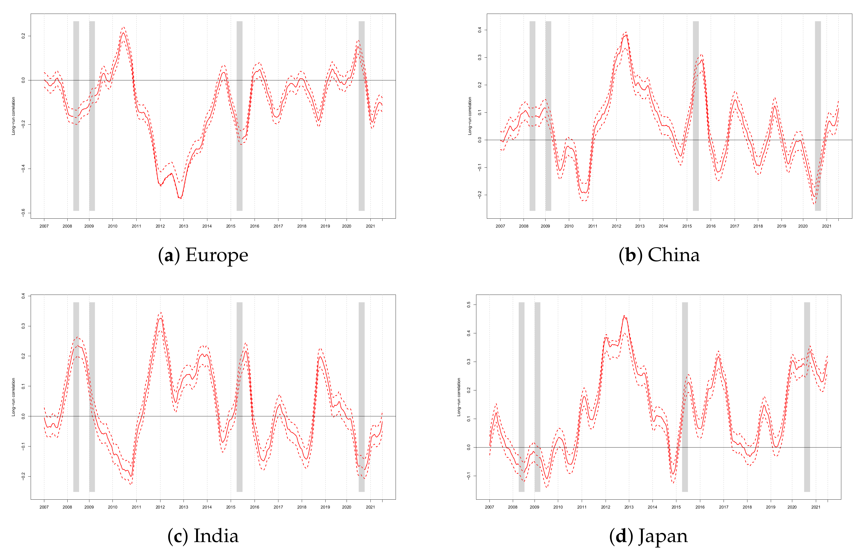
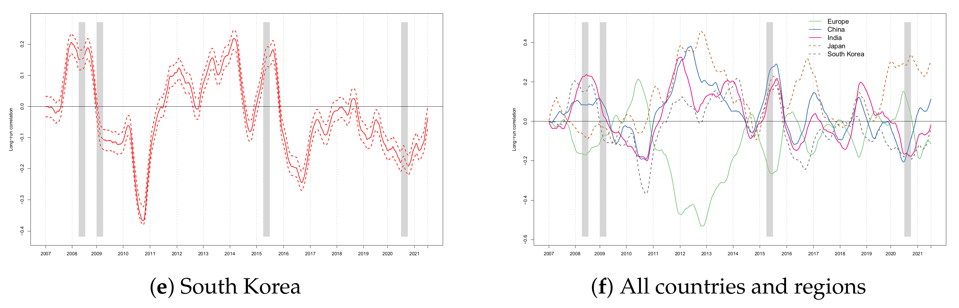
3.2. Lagged Correlations

Hence, let us examine lagged correlations of exchange rates and WTI crude oil log-returns. In Figure 7 and Figure 8 we present the results of the DCC-EGARCH-MIDAS model for oil-exporting countries. It is interesting to note that mostly correlations fluctuate around zero except for Russia and Canada. Correlations for these two countries, just like for the case of contemporaneous correlations, stand out from the rest of the countries and display a very similar declining trend. Such a result infuses some optimism concerning incorporation of these correlations into stock market trading strategies.

Figure 9 and Figure 10 display the results of the DCC-EGARCH-MIDAS model on lagged correlations for oil-importing countries. Except for Europe, correlations of all the other countries show even better co-movement than oil-exporting countries.

4. Conclusions

In the previous section, we saw that both the oil-exporting and oil-importing countries and regions generally react similarly to economic and natural events, with the exception of Europe. In this section, we attempt to provide some economic explanations for the pattern of the correlations between the exchange rates and WTI crude oil log-returns. We mainly focus on two events: the Great Recession period and the COVID-19 pandemic. After the financial collapse of 2008, the WTI crude oil price plummeted. Afterwards, there was a long recovery period until 2012, when oil prices again rose above 100 US dollars per barrel. Such a formidable growth resulted in positive correlations of exchange rates and WTI crude oil returns almost for all oil-exporting countries, which is slightly counterintuitive, since the classical economic theory states that there should be a negative connection. Such negative connection is usually explained by economists as follows: when the oil price goes down the domestic currency market lacks foreign currency supply, which naturally drives national currency down and vice versa [36]. However, as a result of our analysis we state that correlations can also be positive for a decent period of time. The same situation can also be observed for lagged correlations, when currency exchange rate depends on previous fluctuations of the oil price. We obtained positive correlations for the period after the Great Recession for most of the analyzed countries. The possible reason for such a phenomenon is that after the crisis countries were increasing the domestic monetary base as oil prices went up, anticipating future increased international currency supply (in this case national currency weakens) and vice versa: when oil prices went down, countries would decrease liquidity, preventing future deficits of international currency (in this case national currency strengthens). Another possible reason is that after the Great Recession, oil-exporting countries were excessively increasing the monetary base to help their economies recover, which coincided with the massive growth of oil prices.

As concerns oil-importing countries, they also experience mostly positive correlations right after the Great Recession; however, afterwards they remain in the negative zone. This statement is also partly valid for lagged correlations. Overall, correlations for oil-importing countries reveal much stronger concordance than oil-exporting countries, which is again counter-intuitive. Judging by our analysis, it seems that oil-importing countries are even more sensitive to oil price changes than oil-exporting ones. What is even more surprising is that correlations remain in the negative zone for the major part of the analyzed time frame. Such a phenomenon can possibly be explained by preventive monetary base emission/withdrawal undertaken by central banks of oil-importing countries.

Generally speaking, we observed that when WTI crude oil experienced steady growth (as after the huge decrease in the aftermath of 2009), the contemporaneous correlations of exchange rates and oil returns were near zero or positive. On the contrary, when oil prices went down (as immediately after the advent of the COVID-19 pandemic) or were flat, correlations were mostly negative. This statement is valid both for oil-importing and oil-exporting countries. If we focus on the common behavior of the oil-exporting and oil-importing countries/regions, some conclusions can be drawn. In terms of contemporaneous correlations, the oil-exporting countries and oil-importing regions (except Europe) share a similar pattern over time. In terms of lagged correlations, the oil-exporting countries that share similar behavior are Saudi Arabia, Iraq, United States, United Arab Emirates, and Nigeria from one side, and Russia and Canada on the other side (mainly from 2015 onwards). As concerns the oil-importing countries/regions, again the lagged correlation of Europe, especially during the euro-debt crisis (where the peaks happened from 2010 onwards), behaves completely differently from the other countries. Thus, we can tentatively assume that analyzed correlations of oil prices and currency exchange rates can be dependent on the dynamics of the oil prices. Sharp falls in the latter induce the negative correlations for oil-exporting countries and a steady growth relaxes their interdependence.

References

1. Bildirici, M.; Guler Bayazit, N.; Ucan, Y. Analyzing crude oil prices under the impact of Covid-19 by using lstargarchlstm. Energies 2020, 13, 2980. [Google Scholar] [CrossRef]
2. Mensi, W.; Reboredo, J.C.; Ugolini, A. Price-switching spillovers between gold, oil, and stock markets: Evidence from the USA and China during the COVID-19 pandemic. Resour. Policy 2021, 73, 102217. [Google Scholar] [CrossRef]
3. Bouri, E.; Demirer, R.; Gupta, R.; Pierdzioch, C. Infectious diseases, market uncertainty and oil market volatility. Energies 2020, 13, 4090. [Google Scholar] [CrossRef]
4. Kilian, L. Not all oil shocks are alike: Disentangling demand and supply shocks in the crude oil market. Am. Econ. Rev. 2009, 99, 1053–1069. [Google Scholar] [CrossRef] [Green Version]
5. Peersman, G.; Van Robays, I. Oil and the euro area economy. Econ. Policy 2009, 24, 603–651. [Google Scholar] [CrossRef]
6. Baumeister, C.; Van Robays, I.; Peersman, G. The Economic Consequences of Oil Shocks: Differences across Countries and Time. In Inflation in an Era of Relative Price Shocks; Reserve Bank of Australia: Sydney, Australia, 2010; pp. 91–128. [Google Scholar]
7. Kilian, L.; Rebucci, A.; Spatafora, N. Oil shocks and external balances. J. Int. Econ. 2009, 77, 181–194. [Google Scholar] [CrossRef] [Green Version]
8. Barnett, A.; Straub, R. What Drives U.S. Current Account Fluctuations; ECB Working Paper Series No. 959, November; European Central Bank: Frankfurt, Germany, 2008. [Google Scholar]
9. Rickne, J. Oil Prices and Real Exchange Rate Movements in Oil-Exporting Countries: The Role of Institutions; Technical Report; Research Institute of Industrial Economics: Stockholm, Sweden, 2009. [Google Scholar]
10. Serven, L.; Solimano, A. Private investment and macroeconomic adjustment: A survey. World Bank Res. Obs. 1992, 7, 95–114. [Google Scholar] [CrossRef]
11. Bagella, M.; Becchetti, L.; Hasan, I. Real effective exchange rate volatility and growth: A framework to measure advantages of flexibility vs. costs of volatility. J. Bank. Financ. 2006, 30, 1149–1169. [Google Scholar] [CrossRef]
12. Kilian, L.; Zhou, X. Oil Prices, Exchange Rates and Interest Rates; Technical Report, CEPR Discussion Paper No. DP13478; CEPR: London, UK, 2019. [Google Scholar]
13. Brahmasrene, T. Crude Oil Prices and Exchange Rates: Causality, Variance Decomposition and Impulse Response. Energy Econ. 2014, 44, 407–412. [Google Scholar] [CrossRef]
14. Beckmann, J.; Czudaj, R.; Arora, V. The Relationship between Oil Prices and Exchange Rates: Theory and Evidence; Technical Report, US Energy Information Administration Working Paper Series; U.S. Department of Energy: Washington, DC, USA, 2017.
15. Fratzscher, M.; Schneider, D.; Van Robays, I. Oil Prices, Exchange Rates and Asset Prices; Technical Report, CESifo Working Paper Series; European Central Bank: Frankfurt, Germany, 2013. [Google Scholar]
16. Kumar, S. Asymmetric impact of oil prices on exchange rate and stock prices. Q. Rev. Econ. Financ. 2019, 72, 41–51. [Google Scholar] [CrossRef]
17. Kim, J.; Jung, H. Dependence Structure between Oil Prices, Exchange Rates, and Interest Rates. Energy J. 2018, 39, 233–258. [Google Scholar] [CrossRef] [Green Version]
18. Blokhina, T.; Karpenko, O.; Guirinskiy, A. The Relationship between Oil Prices and Exchange Rate in Russia. Int. J. Energy Econ. Policy 2014, 6, 721–726. [Google Scholar]
19. Hasanov, F.; Mikayilov, J.; Bulut, C.; Suleymanov, E.; Aliyev, F. The role of oil prices in exchange rate movements: The CIS oil exporters. Economies 2017, 5, 13. [Google Scholar] [CrossRef] [Green Version]
20. Reboredo, J.C. Modelling oil price and exchange rate co-movements. J. Policy Model. 2012, 34, 419–440. [Google Scholar] [CrossRef]
21. Beckmann, J.; Czudaj, R.L.; Arora, V. The relationship between oil prices and exchange rates: Revisiting theory and evidence. Energy Econ. 2020, 88, 104772. [Google Scholar] [CrossRef]
22. Engle, R.F. Dynamic conditional correlation: A simple class of multivariate generalized autoregressive conditional heteroskedasticity models. J. Bus. Econ. Stat. 2002, 20, 339–350. [Google Scholar] [CrossRef]
23. Colacito, R.; Engle, R.F.; Ghysels, E. A component model for dynamic correlations. J. Econom. 2011, 164, 45–59. [Google Scholar] [CrossRef] [Green Version]
24. Ghysels, E.; Sinko, A.; Valkanov, R. MIDAS regressions: Further results and new directions. Econom. Rev. 2007, 26, 53–90. [Google Scholar] [CrossRef]
25. Filis, G.; Degiannakis, S.; Floros, C. Dynamic correlation between stock market and oil prices: The case of oil-importing and oil-exporting countries. Int. Rev. Financ. Anal. 2011, 20, 152–164. [Google Scholar] [CrossRef]
26. Nelson, D.B. Conditional heteroskedasticity in asset returns: A new approach. Econometrica 1991, 59, 347–370. [Google Scholar] [CrossRef]
27. Candila, V. Multivariate Analysis of Cryptocurrencies. Econometrics 2021, 9, 28. [Google Scholar] [CrossRef]
28. Asgharian, H.; Christiansen, C.; Hou, A.J. Macro-finance determinants of the long-run stock–bond correlation: The DCC-MIDAS specification. J. Financ. Econom. 2015, 14, 617–642. [Google Scholar] [CrossRef]
29. Yang, L.; Yang, L.; Ho, K.C.; Hamori, S. Determinants of the long-term correlation between crude oil and stock markets. Energies 2019, 12, 4123. [Google Scholar] [CrossRef] [Green Version]
30. Sebai, S.; Naoui, K.; ben brayek, A. A study of the interactive relationship between oil price and exchange rate: A copula approach and a DCC-MGARCH model. J. Econ. Asymmetries 2015, 12, 173–189. [Google Scholar] [CrossRef]
31. Yang, L.; Cai, X.J.; Hamori, S. What determines the long-term correlation between oil prices and exchange rates? N. Am. J. Econ. Financ. 2018, 44, 140–152. [Google Scholar] [CrossRef]
32. Amano, R.A.; Van Norden, S. Oil prices and the rise and fall of the US real exchange rate. J. Int. Money Financ. 1998, 17, 299–316. [Google Scholar] [CrossRef]
33. John, M.; Wu, Y.; Narayan, M.; John, A.; Ikuta, T.; Ferbinteanu, J. Estimation of dynamic bivariate correlation using a weighted graph algorithm. Entropy 2020, 22, 617. [Google Scholar] [CrossRef]
34. Choi, J.E.; Shin, D.W. Nonparametric estimation of time varying correlation coefficient. J. Korean Stat. Soc. 2021, 50, 333–353. [Google Scholar] [CrossRef]
35. Candila, V. dccmidas: A Package for Estimating DCC-Based Models in R. R Package Version 0.1.0. 2021. Available online: https://www.researchgate.net/publication/350064227_dccmidas_A_package_for_estimating_DCC-based_models_in_R (accessed on 24 August 2021).
36. Jawadi, F.; Louhichi, W.; Ameur, H.B.; Ftiti, Z. Do Jumps and Co-jumps Improve Volatility Forecasting of Oil and Currency Markets? Energy J. 2019, 40, SI2. [Google Scholar] [CrossRef]
Figure 1. Exchange rates of the top-seven oil-exporting countries and WTI crude oil price. Notes: The figure depicts the patterns in the exchange rates (from (ag)) and WTI crude oil (h). Sample period: January 2007 to June 2021. Number of observations: 3563.
Energies 14 08046 g001
Figure 2. Exchange rates of the top-five oil-importing countries (or region) and WTI crude oil price. Notes: The figure depicts the patterns in the exchange rates (from (ae)) and WTI crude oil (f). Sample period: January 2007 to June 2021. Number of observations: 3563.
Energies 14 08046 g002
Figure 3. Volatilities and contemporaneous correlations for exchange rates of oil-exporting countries and WTI crude oil returns. Notes: Plots of volatilities (main diagonal) and contemporaneous correlations. Sample period: January 2007 to June 2021. Number of observations: 3563.
Energies 14 08046 g003
Figure 4. Contemporaneous correlations among exchange rates and WTI crude oil returns. Oil-exporting countries. Notes: The plots from (ag) depict the time-varying long-run contemporaneous correlations among exchange rates of the oil-exporting countries and WTI crude oil returns (solid red lines) as well as their 95% confidence intervals (dashed red lines). The plot in (h) jointly illustrates all the time-varying long-run contemporaneous correlations. Shaded areas are the key geopolitical and economic events defined by the EIA. These events are global financial collapse (2008, Q2), OPEC production targets cut (2009, Q1), OPEC production quota unchanged (2015, Q2), and global pandemic oil demand reduction (2020, Q3). Sample period: January 2007 to June 2021. Number of observations: 3563.
Energies 14 08046 g004aEnergies 14 08046 g004b
Figure 5. Volatilities and contemporaneous correlations for exchange rates of oil-importing countries and WTI crude oil returns. Notes: Plots of volatilities (main diagonal) and contemporaneous correlations. Sample period: January 2007 to June 2021. Number of observations: 3563.
Energies 14 08046 g005
Figure 6. Contemporaneous correlations among exchange rates and WTI crude oil returns. Oil-importing countries. Notes: The plots from (ae) depict the time-varying long-run contemporaneous correlations among exchange rates of the oil-importing countries and WTI crude oil returns (solid red lines) as well as their 95% confidence intervals (dashed red lines). The plot in (f) jointly illustrates all the time-varying long-run contemporaneous correlations. Shaded areas are the key geopolitical and economic events defined by the EIA. These events are global financial collapse (2008, Q2), OPEC production targets cut (2009, Q1), OPEC production quota unchanged (2015, Q2), and global pandemic oil demand reduction (2020, Q3). Sample period: January 2007 to June 2021. Number of observations: 3563.
Energies 14 08046 g006aEnergies 14 08046 g006b
Figure 7. Volatilities and lagged correlations for exchange rates of oil-exporting countries and WTI crude oil returns. Notes: Plots of volatilities (main diagonal) and lagged correlations. Sample period: January 2007 to June 2021. Number of observations: 3563.
Energies 14 08046 g007
Figure 8. Lagged correlations among exchange rates and WTI crude oil returns. Oil-exporting countries. The plots from (ag) depict the time-varying long-run lagged correlations among exchange rates of the oil-exporting countries and WTI crude oil returns (solid red lines) as well as their 95% confidence intervals (dashed red lines). The plot in (h) jointly illustrates all the time-varying long-run lagged correlations. Shaded areas are the key geopolitical and economic events defined by the EIA. These events are global financial collapse (2008, Q2), OPEC production targets cut (2009, Q1), OPEC production quota unchanged (2015, Q2), and global pandemic oil demand reduction (2020, Q3). Sample period: January 2007 to June 2021. Number of observations: 3563.
Energies 14 08046 g008
Figure 9. Volatilities and lagged correlations for exchange rates of oil-importing countries and WTI crude oil returns. Notes: Plots of volatilities (main diagonal) and lagged correlations. Sample period: January 2007 to June 2021. Number of observations: 3563.
Energies 14 08046 g009
Figure 10. Lagged correlations among exchange rates and WTI crude oil returns. Oil-importing countries. The plots from (ae) depict the time-varying long-run lagged correlations among exchange rates of the oil-importing countries and WTI crude oil returns (solid red lines) as well as their 95% confidence intervals (dashed red lines). The plot in (f) jointly illustrates all the time-varying long-run lagged correlations. Shaded areas are the key geopolitical and economic events defined by the EIA. These events are global financial collapse (2008, Q2), OPEC production targets cut (2009, Q1), OPEC production quota unchanged (2015, Q2), and global pandemic oil demand reduction (2020, Q3). Sample period: January 2007 to June 2021. Number of observations: 3563.
Energies 14 08046 g010aEnergies 14 08046 g010b