Will Aggregator Reduce Renewable Power Surpluses? A System Dynamics Approach for the Latvia Case Study

Abstract

Power demand-side management has been identified as one of the possible elements towards a more flexible power system in case of increased capacities of variable renewable energy sources—solar and wind energy. The market coordinators or aggregators are introduced to adjust the electricity consumption by following the market situation. However, the role of aggregators is mainly analysed from the economic perspective, and the demand side management is performed to maximise the utilisation of low price power during off-peak hours. However, this research focuses on analysing the introduction of aggregators as a future player to increase the total share of renewable power and decrease the surplus solar and wind electricity occurrence. An in-depth system dynamics model has been developed to analyse the hourly power production and power consumption rates at the national level for the Latvia case study. The results show that introducing aggregators and load shifting based on standard peak shaving can increase the share of surplus power and does not benefit from increased utilisation of solar and wind power. On the contrary, demand-side management based on available RES power can decrease the surplus power by 5%.

1. Introduction

On the European Union’s (EU) way towards climate neutrality, the role of renewable energy sources (RES) keeps growing. However, the volatile nature of the RES, which depends on the wind speed, solar radiation, water inflow in rivers, also requires a higher level of flexibility in the energy demand. One of the solutions for providing flexibility is to involve demand response. As has been defined in the EU Directive on standard rules for the internal electricity market (Electricity Directive), demand response (DR) is “the change of electricity load by final customers from their normal or current consumption patterns in response to market signals” [1]. Thus, in DR, electricity consumers provide adjustments in their regular electricity consumption.

There are four main reasons for DR [2]:

(1)

To reduce the total electricity consumption;

(2)

To reduce the need for more power generation;

(3)

To change the demand pattern to stimulate the potential of renewable energy generation;

(4)

To reduce the congestion risks in the electricity grid.

DR is usually facilitated by a new electricity market participant—an aggregator who performs aggregation [3,4]. As has been defined in the Electricity Directive, aggregation is “a function performed by a natural or legal person who combines multiple customer loads or generated electricity for sale, purchase or auction in any electricity market” [1]. In reality, it means that this electricity market player—the aggregator—has agreements with electricity consumers, who should adjust their electricity consumption following the instructions of the aggregator, who follows the market situation and requests energy consumption to be decreased when the electricity demand and price is high (during the peak hours) and the consumption to be increased when the electricity demand and price are lower. In return, it provides financial savings for the consumer [5]. Meanwhile, demand response provides both financial benefits for the consumer and security of energy supply due to the uncertain nature of RES and the necessity to optimise the energy consumption [6,7].

DR can be applied both to residential and industrial consumers; however, the electricity consumption load from a residential consumer is relatively minor. Therefore, aggregators need to involve a high level of residential participation in the DR to impact the electricity market [8]. This aspect has also been overviewed in the case study for Latvia while discussing that currently, there are no active aggregators in the Latvian electricity market [4]. Research from Germany shows that 80% of the electricity is consumed by around 2–10% of the industrial consumers [9]. A similar situation has been identified in Latvia, where 85% of electricity is consumed by 25% of the industrial consumers, specifically by the manufacturing sector, providing good opportunities for aggregation [10]. For industrial consumers, the most typical high electricity load to control is considered air conditioning and heating, ventilation, and air conditioning systems, which are simple to control by distance (i.e., with smart metering) and provide large load DR at once in comparison to individual household loads [9]. Some studies differentiate between DR aggregator for residential, commercial, industrial, and agricultural activities and DR by prosumers, small energy producers, producing for their consumption [11].

Though DR has not yet been developed in Latvia, the corresponding national legislative framework has been developed. Nevertheless, it is not fully compliant with the Electricity Directive and provides barriers for independent aggregators to enter the market, as they have to coordinate their actions with electricity suppliers [12].

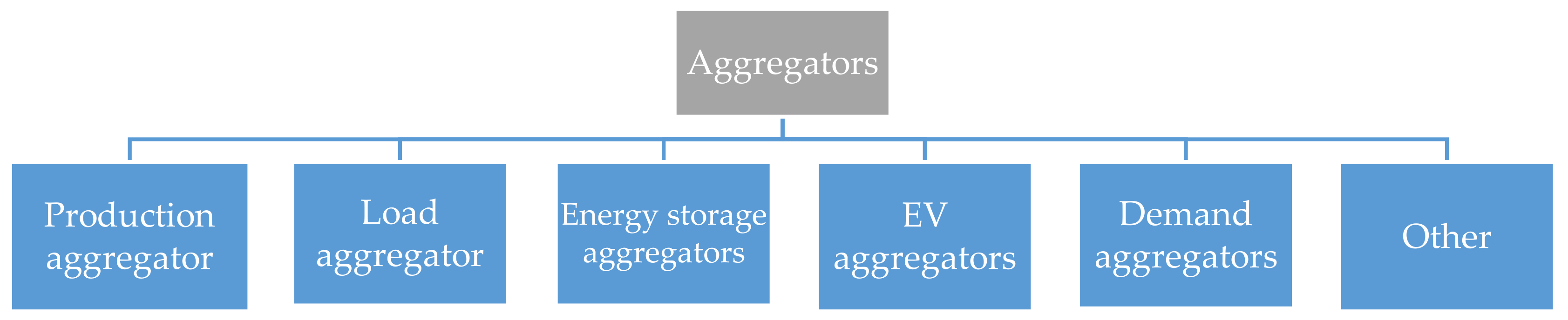
Aggregators can be assigned into different categories depending on the source of aggregated energy, as shown in Figure 1. but they are not limited to that. Demand aggregator can be the electricity supplier and aggregate electricity from all its consumers. The load aggregator aggregates flexibility. The production aggregator aggregates electricity from a group of generators, i.e., electricity producers are asked to increase or reduce generation loads at their power plant [13]. Electric vehicles can participate in aggregation by charging or discharging their batteries into the grid [14]. The same goes for energy storage. The location of the consumers is not essential [8].

Aggregators can play a large set of roles in providing flexibility in the energy market, as they can aid different electricity market players, such as reducing imbalances in the electricity system or avoiding congestions in the electricity grid [15].

A study shows that an aggregator in principle can have three types of contracts with its consumers:

(a)

Fixed load—a load that cannot be reduced or shifted by the aggregator and has to be constant during a specific time frame to keep the consumers’ activities intact;

(b)

Load curtailment—a load that has to be reduced when aggregator requests it;

(c)

Duration differentiated loads—a load has to be provided at certain time frames for a specific duration in a certain amount of time. Thus, it is not a continuous load, which differs from a fixed load [16].

The types of contracts mentioned above can be further elaborated into specific strategies. Aggregators can provide DR by implementing different demand-side management strategies [4,17]. For example, while peak clipping reduces the energy consumption, valley filling stipulates the consumption at other times of the day, most commonly by charging batteries such as for the EV [18]. The strategies can be combined to adjust to the electricity generation at a given time. The most common strategy is load shifting, where high electricity demand is lowered by shifting it to another time of the day. Thus, the peak demand is curtailed while this demand is shifted. The load can be shifted as a whole, but it can also be subdivided into smaller loads and spread across a specific period.

For aggregators to provide their services, the consumer should have a smart meter. Though system operators provide gradual roll-out of smart meters, aggregators provide their technologies to control the consumer’s appliances from a distance [19]. Thus, the consumer technically does not have to control its appliances. The aggregator can do it on behalf of the consumer, e.g., switching off the air-conditioner at a certain point and turning it back on after a short period so the consumer cannot feel discomfort.

Two types of DR programs can be distinguished as providing consumer benefits–incentive-based and price-based programs. An incentive-based program pays a fee to consumers for reducing the electricity demand at peak hours. But price-based program provides different electricity prices at different times. Thus consumers would choose to consume electricity at times when the prices are lower [17]. If the consumer has a dynamic price agreement with its electricity supplier, it gains a monthly fee from the aggregator (as per their agreement) and lowers the monthly electricity bill costs.

Aggregators can participate both in the day-ahead market by providing a bid on how much DR it is willing to provide on the next day and in the balancing market to ensure the real-time stability in the electricity market after other market participants have failed to fulfil their commitment in the day-ahead market. However, it needs to be noted that aggregators themselves can also fail to fulfil their bids and can provide imbalances in the market. Moreover, aggregators can cause imbalance to other market participants due to their activities [4,20].

To provide services in the electricity market, aggregator uses decision-support tools. These can be optimisation models that show the day-ahead bids and real-time optimisation algorithms that allow the aggregator to follow the flexibility and provide the load trade by aggregators in the day-ahead markets. If an aggregator plans to provide multiple products (balancing energy, reserves etc.) to the market, there are also tools to support that by controlling in real-time diverse, flexible resources [21]. Research shows that a support vector machine (statistical learning approach) can be used with relatively high accuracy to forecast the loads aggregated from households [22]. Different game models have been developed (both with regulated and unregulated competition and using Nash equilibrium) to model the competition between multiple aggregators, which provide each aggregator with the best bidding strategy to benefit the most [21]. The same game models have also been used to show the benefit for system operators arising from aggregators’ services [23]. Meanwhile, the mathematical modelling of DR algorithms shows the effect of DR activation at different levels—household level, grid level, and wholesale market level [24]. There have also been researched particular methods for using DR for residential consumption in smart grids with a high level of renewable energy coming into the market, providing the optimal usage of renewable energy, where consumption with the aid of aggregators could follow the renewable energy production load [25,26].

The above reviewed EU legal framework and academic research provides us with the general concept of DR and outline the role aggregators could play in the energy market. However, the actual effect of aggregation depends on the circumstances in the specific EU country, where the aggregation is applied considering such previously mentioned aspects as electricity consumption patterns, electricity generation loads, availability of smart meters, consumers’ willingness to participate in DR (including policy incentives), national legal framework, etc. Thus, the article focuses on analysing the possible benefits of DR on reaching a higher renewable power share in the power market of Latvia. An in-depth system dynamics model compares the hourly power consumption and RES power production rates to identify the potential flexibility increase through the introduction of aggregators and obtained environmental benefits from the increased utilisation of RES power in Latvia.

2. Materials and Methods

The system dynamics modelling method evaluates the dynamic effects of DR and its future role in the national energy sector. Modelling is performed by using the Stella Architect software (Stella Architect 2.1. developed by isee systems, Lebanon, NH, USA). This method is broadly applied to analyse different aspects of the energy sector, including energy efficiency increase, RES support policies, and innovative heat supply techniques [27,28,29].

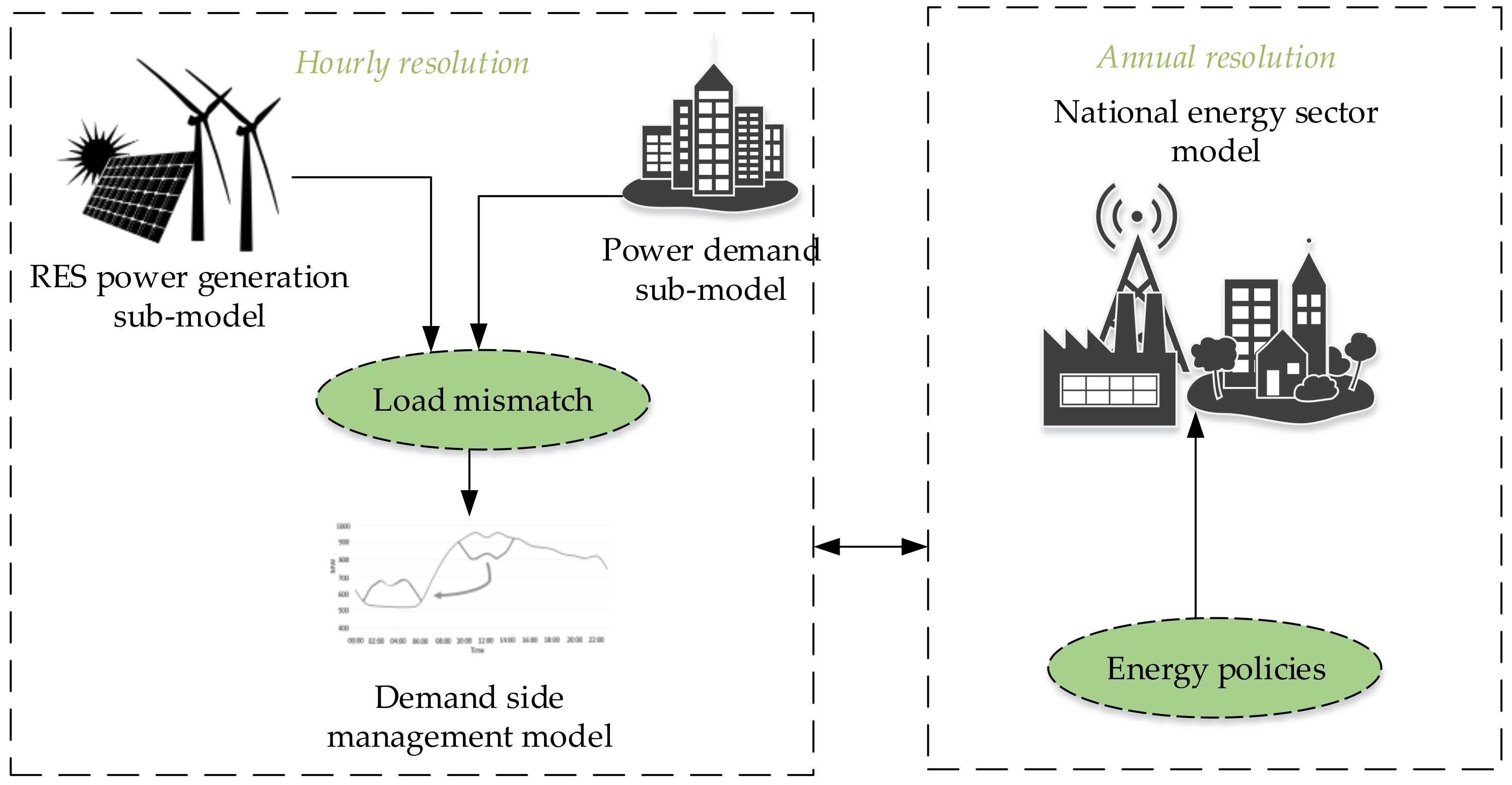
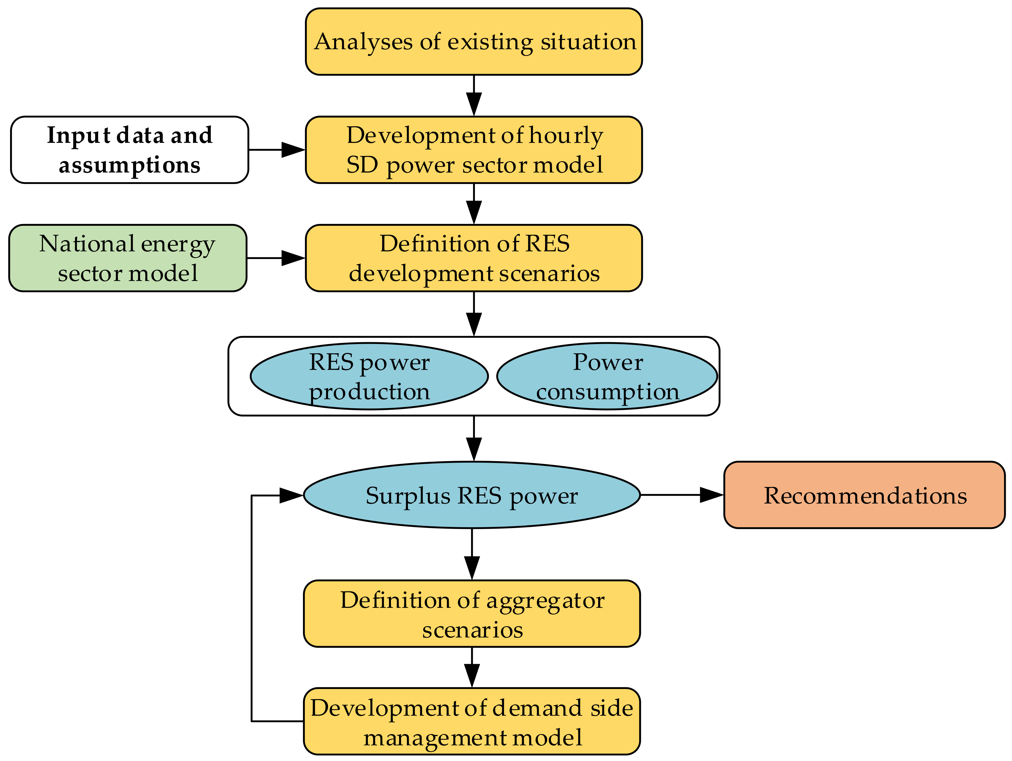
Figure 2 shows the overall concept of the study. The research algorithm is shown in Figure 3. The first step includes the analysis of an existing situation in the power sector and developing a system dynamics model on an hourly basis. The hourly RES power generation and demand submodel is soft-linked to the national energy system model by providing the annual input data regarding the RES power. The national model represents the overall situation in the Latvia case study and includes different energy consumers and producing units. The installed capacity of the RES power systems has been obtained from the national energy sector model, which also included different support policies promoting RES installations. The hourly solar and wind power generation has been compared with the average power demand profile in the household, industrial and service sectors by identifying the periods when surplus power occurs.

Further, the load mismatch has been analysed, and different scenarios for demand-side management strategies and aggregator roles in the energy sector have been evaluated. The aggregator has been introduced within the study to increase the overall system flexibility towards higher integrated RES power share. The surplus power amount is recalculated for the scenarios with aggregator introduction. The results are compared with the base scenario without demand-side management. Finally, the conclusions and recommendations for power sector flexibility increase are identified.

2.1. Power Sector in Latvia

The most significant sources of electricity generation in Latvia are two natural gas thermal power plants with a total installed capacity of 976 MW and large hydroelectric power plants along the river Daugava with a total installed capacity of 1558 MW. Other sources consist of a total of 212 MW installed capacity, including smaller producers with 203 MW installed capacity such as cogeneration plants, hydroelectric power plants, solar power plants, and wind turbines [30]. An additional amount of power is produced in microgeneration that mainly consists of solar power plants with nine MW of installed capacity [30]. By producing electricity locally, Latvia had around a 15% shortage in 2018, covered by power imports.

Power consumption mainly consists of three sectors, production, services, and households. The services sector has the highest electricity consumption share of 42%, following production with 30% and households with 28% in 2020. From 2008 to 2020, household electricity consumption has been decreasing, while electricity consumption from services has fluctuated [31].

Latvia participates in the Nord Pool day-ahead market, an auction where power is traded for delivery each hour of the next day [32]. Nord Pool markets are divided into several bidding areas. Based on the submitted orders bidding area prices are calculated and published. Therefore, power is always transferred from the low price area to the high price area. The resulting energy prices and demand indicate how much electricity should be produced locally, exported, or imported [33].

2.2. Power Consumption Modelling

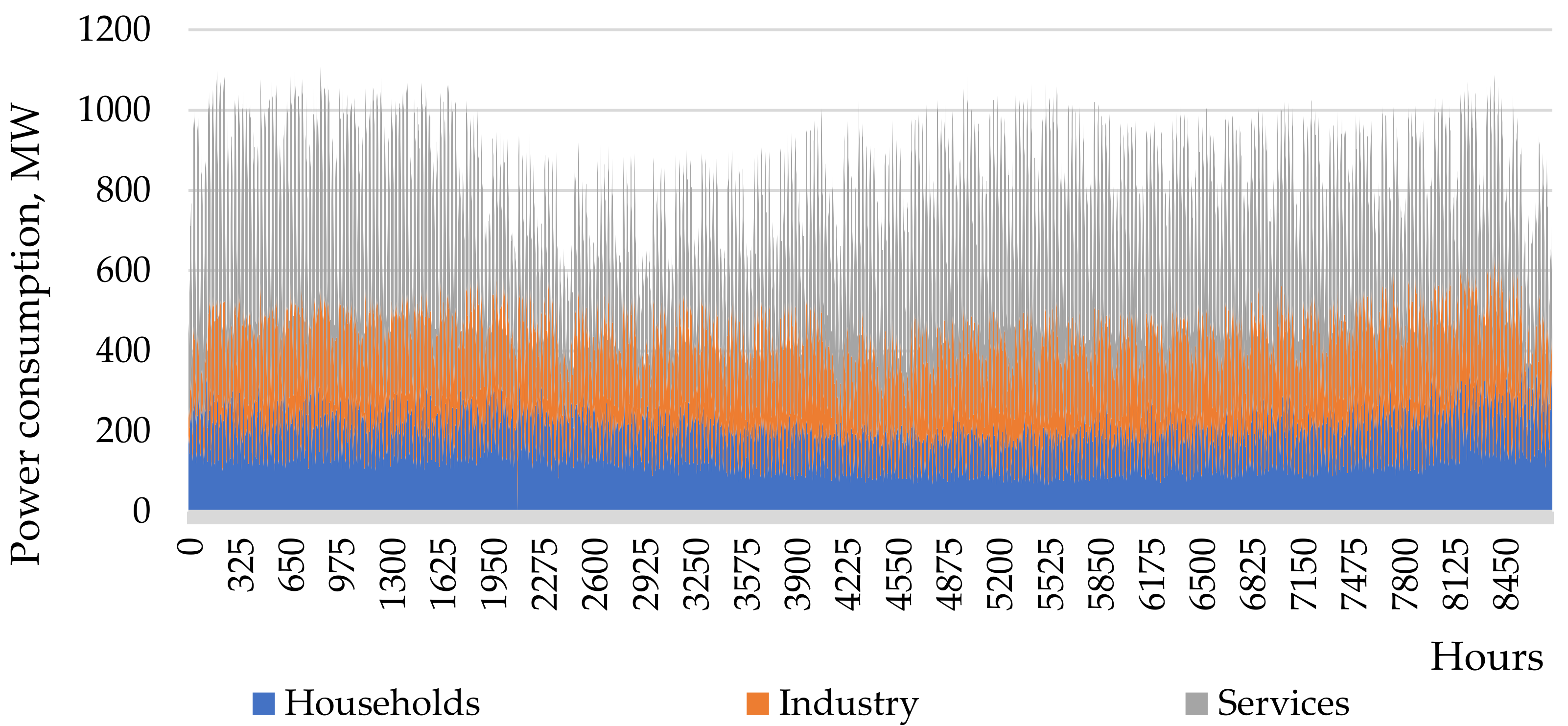
The primary variable for successful aggregator operation is power consumption. Therefore, the hourly power consumption data have been used as the main parameter to model the potential load shifting. Hourly consumption profile for different consumers is acquired from the electricity distribution operator of Latvia [34]. The model uses the average hourly power consumption from 70 households with total annual power consumption ranging from 1.8 MWh to 18 MWh per year and 50 industrial and service consumers in 2018. The industrial consumers include wood processing, the food industry and other industrial plants, with the annual power consumption ranging from 189 MWh to 8060 MWh per year. The consumers from the service sector include 25 different public and private utilities, including banks, hospitals, shopping malls, educational buildings etc. 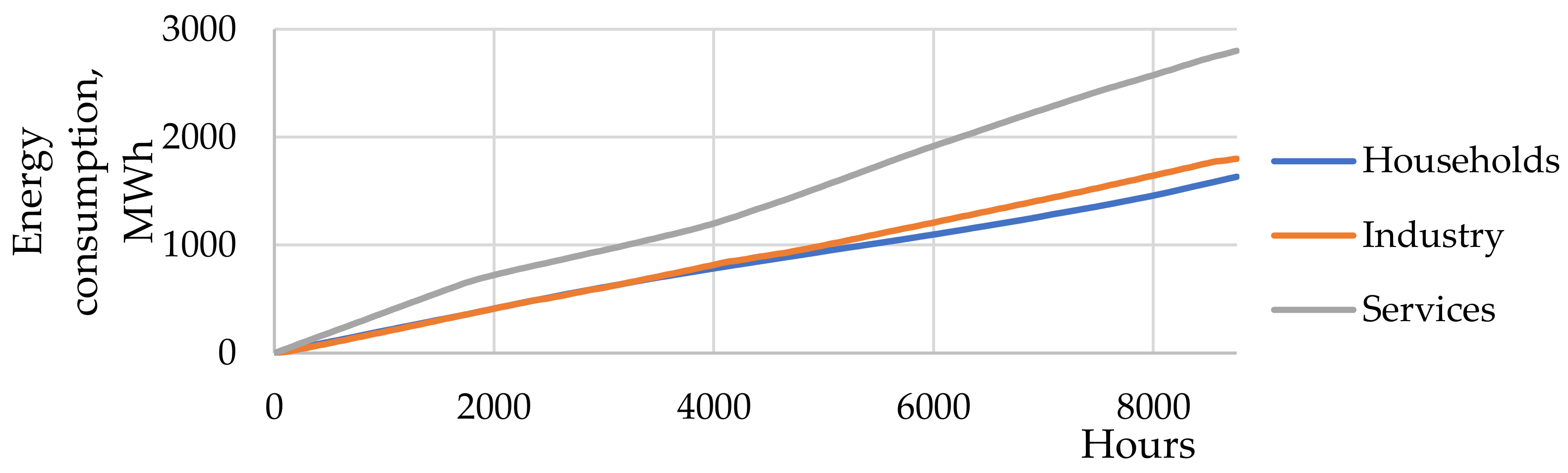As a result, the annual consumption in the service sector varies from 54 MWh per year to 1972 MWh.The average profile is calculated from the provided sample of consumption profiles for each consumer group (see Figure 4.). Then, the average profile is attributed to all consumers in each group to calculate total electricity consumption in household, industry and services sectors.

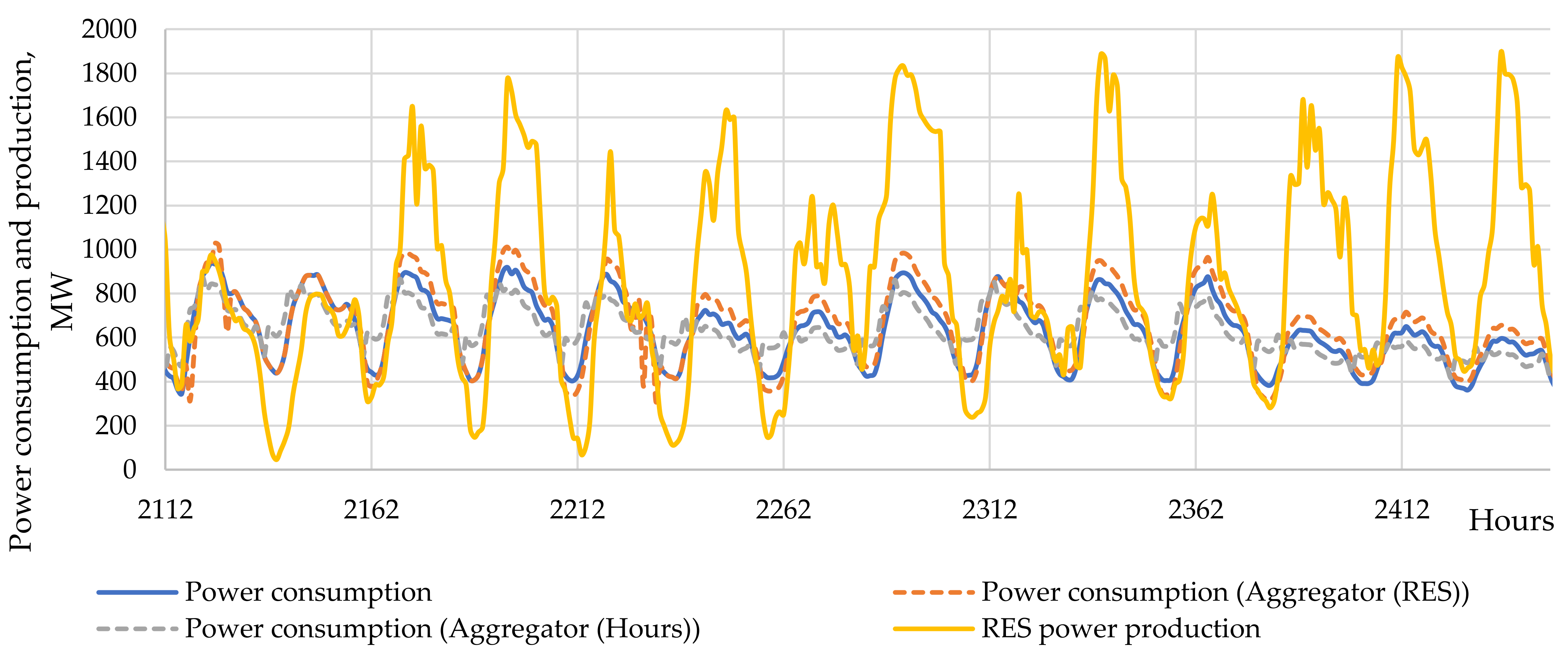
The final results are compared to the statistics of electricity consumption in each sector at the national level. Annual consumption of electricity for different consumers are taken from official statistics [35]. Figure 5. displays the accumulated electricity consumption based on hourly consumption profiles.

From the actual power consumption data, the peak hours and the power consumption at night have been estimated.

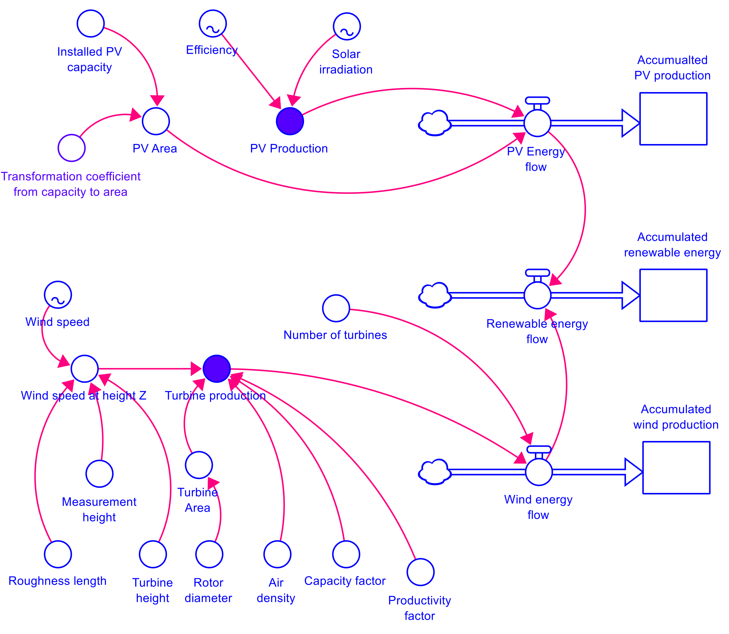
2.3. RES Power Production Sub-Model

The RES power production sub-model (see Figure 6.) estimates the hourly power production rates from wind farms and solar power plants based on climatic conditions in Latvia.

The solar power production rates are based on the average solar irradiation data and assumptions on average photovoltaic (PV) panel efficiency [36]:

$$E_{PV}={\mathsf{\eta }}_{PV}·SI$$

(1)

where E_PV—PV power production, MW/h; S_PV—installed area of PV, m²; η_PV—PV efficiency, %; SI—solar irradiation, MW/m²/h.

The data regarding average solar irradiation rates from 2018 have been used within the model obtained from the national meteorological database. More in-depth analysis regarding solar profiles in Latvia has been described in previous research by Polikarpova et al. [37]. In July, the maximal hourly solar irradiation reaches 799 W/m², but the average annual solar irradiation is 1002 kWh/m².

The hourly production rates of wind power are based on the average hourly wind speed and general estimations on technical parameters of typical wind turbines. The hourly wind power capacities are calculated according to (2):

$$E_{WT}=\frac{0.5\times C_f\times \mathsf{\eta }\times {\rho }_{air}\times A\times v_z{}^3}{\mathrm{1,000,000}}$$

(2)

where E_WT—turbine production, MW/h C_f—capacity factor; $\mathsf{\eta }$—productivity factor; ${\rho }_{air}$—air density, kg/m³; A—Rotor area, m²; v_z—wind speed at wind turbine height, m/s.

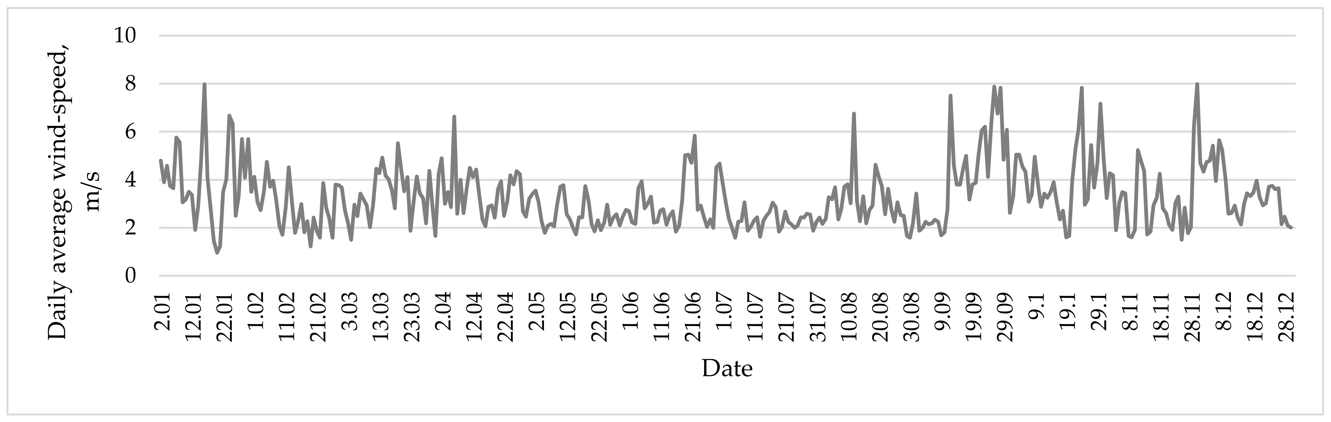
The hourly wind speed data from the year 2018 have been used for the calculation. The average wind speed in Latvia at measured 2 m height is 3.4 m/s. As it can be seen in Figure 7, higher wind speed fluctuations are observed during autumn and winter periods. In addition, the limitations have been added for the hours above the cut-off speed above 6 m/s as the wind turbines should be stopped in order to prevent unnecessary strain on the rotor [38].

The following equation calculates the wind speed at wind turbine height:

$$v_z=\frac{v_{ref·ln\frac{z}{z_0}}}{ln\frac{z_{ref}}{z_0}}$$

(3)

where v_ref—wind speed in reference height, m/s; z—wind turbine height, m; z_ref—the height of wind speed measurements, m; z₀—roughness length, m.

The following equations calculate the flow of the hourly production from installed wind and solar technology capacities:

$$E_{Wind}=E_{WT}·N_{WT}$$

(4)

$$E_{Solar}=E_{PV}·S_{PV}$$

(5)

$$E_{RES}=E_{Wind}+E_{Solar}$$

(6)

where E_Wind—hourly wind energy production, MW/h; N_WT—number of turbines installed; E_Solar—hourly solar energy production, MW/h, S_PV—installed area of PV, m²; E_RES—hourly RES production, MW/h.

Accumulated production stock value for each of the renewable technology at any given time can be calculated by the following equation:

$$S{t}_i\left(t\right)={{\displaystyle \int }}_{t_0}^t(F{l}_i)dt+S{t}_i\left(t_0\right)$$

(7)

where St_i—accumulated energy production of specific technology, MWh; Fl_i—hourly energy production of specific technology, MW/h.

The main technical assumptions for RES power estimations are summarised in

Table 1. The main technical assumptions for RES technologies.

Parameter	Assumption
PV efficiency, ηPV	0.18
Capacity factor, Cf	0.4
Productivity factor, η	0.4
Rotor diameter, m	60
Wind turbine high, m	70
High for wind speed measurements, m	2.5
Roughness length, m	0.15

based on the average values from technical catalogues of different technologies [39]. Based on the specifications of ongoing development projects in Latvia, it has been assumed that wind turbines with a height of 70 m and a rotor diameter of 60 m could be the most reliable solution. In addition, the climatic data regarding hourly wind speed rates and solar irradiation have been obtained from the national meteorological data centre database [40].

The total area of installed solar panels and wind turbines is estimated based on the forecasted amount of national RES capacities. Overview of installed capacities of variable RES technologies is displayed in

Table 2. Installed capacities of variable renewable energy (VRE) sources in different scenarios.

	Solar Capacity, MW	Wind Capacity, MW
Scenario 1	0	77
Scenario 2	100	500
Scenario 3	149	964
Scenario 4	964	149

.

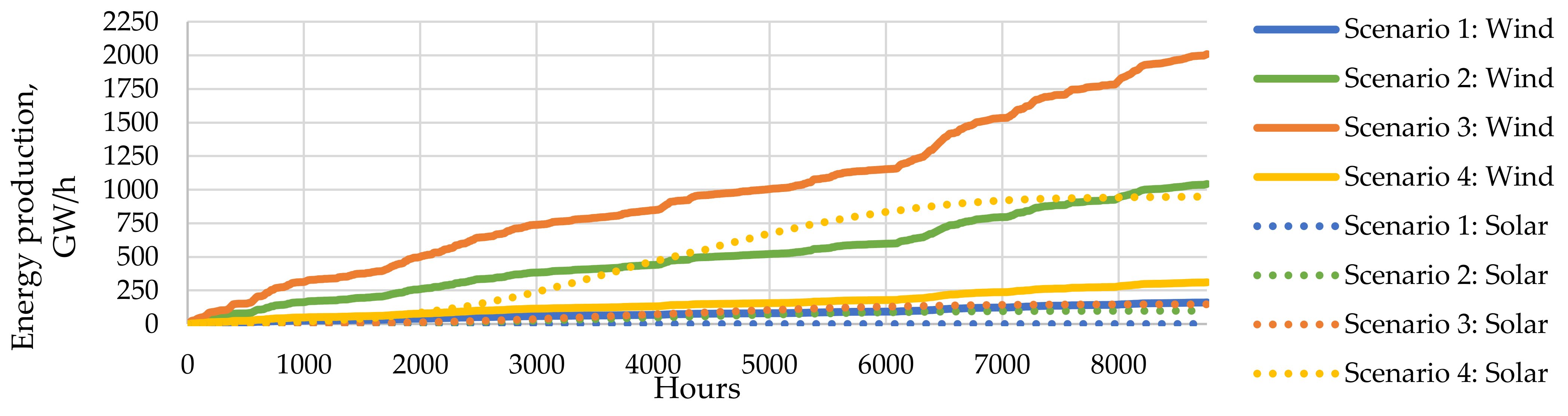
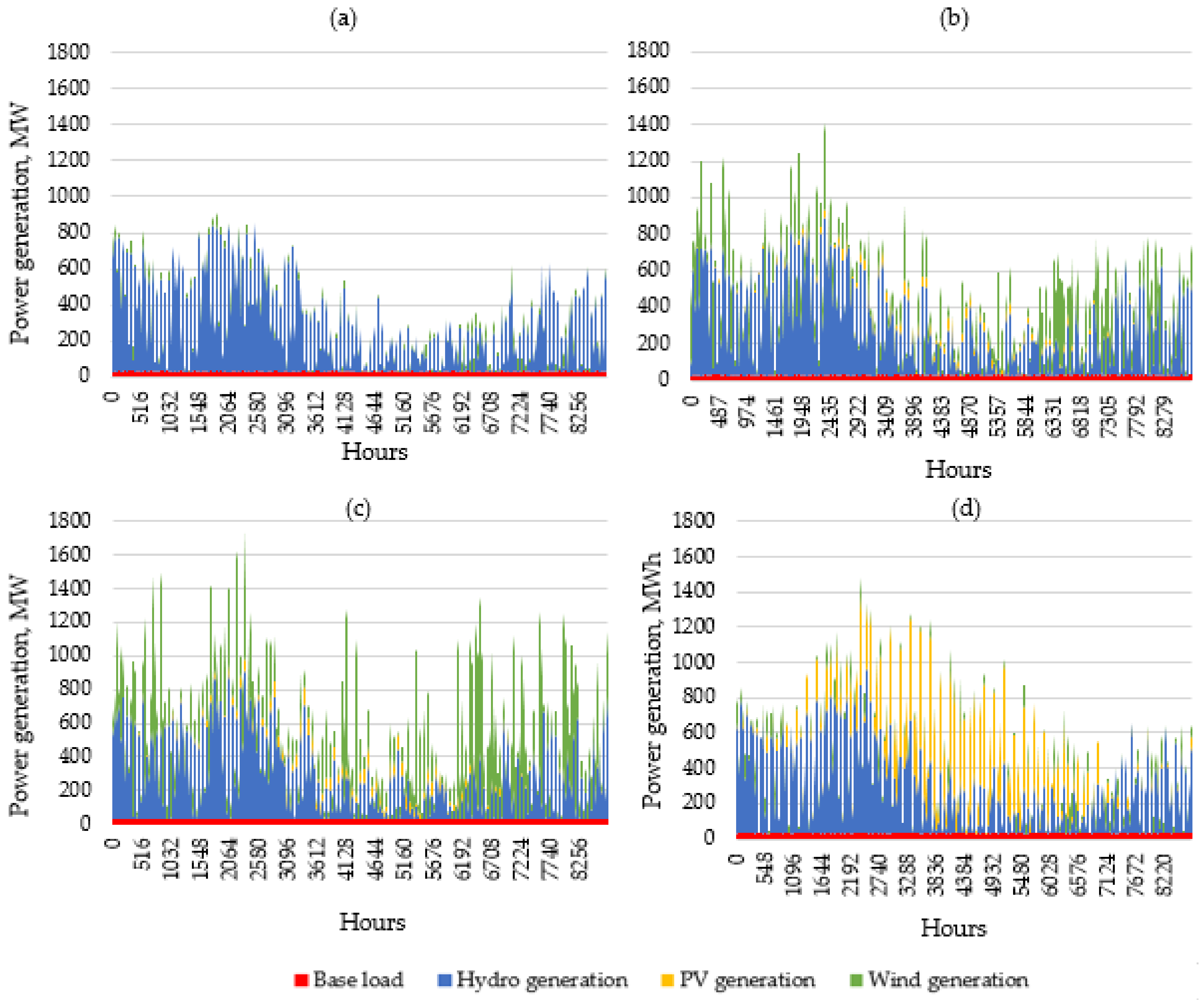
In this study, four different solar and wind technology capacity combinations were tested. Scenario 1 describes Latvia’s current situation when no large solar power plants are installed, and only a few wind farms are operating. Scenario 2 and 3 values represent the medium and optimistic forecast of Latvia’s solar and wind technology development until 2050. The forecast was obtained by using the previously developed national scale energy sector model [41]. The model forecasts the future development of RES technologies based on the existing situation, as well as analyses driving forces (development of technologies and price reductions, increase of fossil fuel prices, energy efficiency increase) and barriers (high investment costs, energy source availability, lack of information, insufficient building capacity). In addition, the model includes the main support policies identified within the National Energy and Climate Plan for 2030, such as subsidies for RES technologies, an increase of tax rates etc. Finally, scenario 4 is an inverted version of Scenario 3 in which forecasted solar and wind capacities are reversed to highlight the impact of the increased capacity of PV panels.

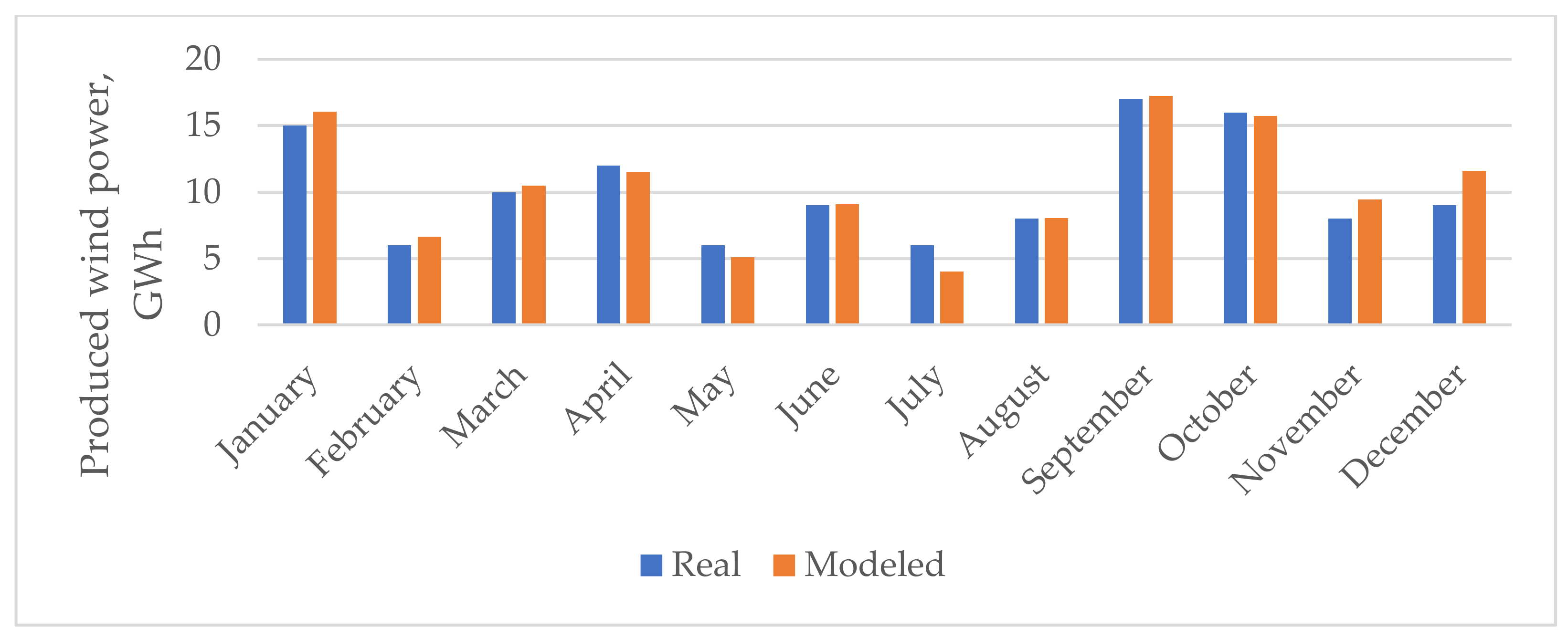
The simulated and real wind generation rates in Scenario 1 (existing situation) in 2018 have been compared to validate the modelling results. The results (see Figure 8) shows that the monthly wind power production rates are similar to those obtained from the system dynamics model. The system dynamics model’s annually generated wind power difference is 2% compared to the actual production rates, which shows the high accuracy of the developed model.

2.4. Modelling of Demand-Side Management and Aggregator

Demand-side management has been introduced to align the RES power production and power consumption profiles. Within the research, two different types of aggregators and demand-side management mechanisms have been tested and compared:

• Load aggregator to balance the power load by shifting peak load to the night hours—Aggregator (Hours);
• Flexibility aggregator to decrease the RES surplus power occurring by shifting the power load to the periods with higher RES production rates—Aggregator (RES).

For each type of aggregator, different approaches have been used for demand-side management.

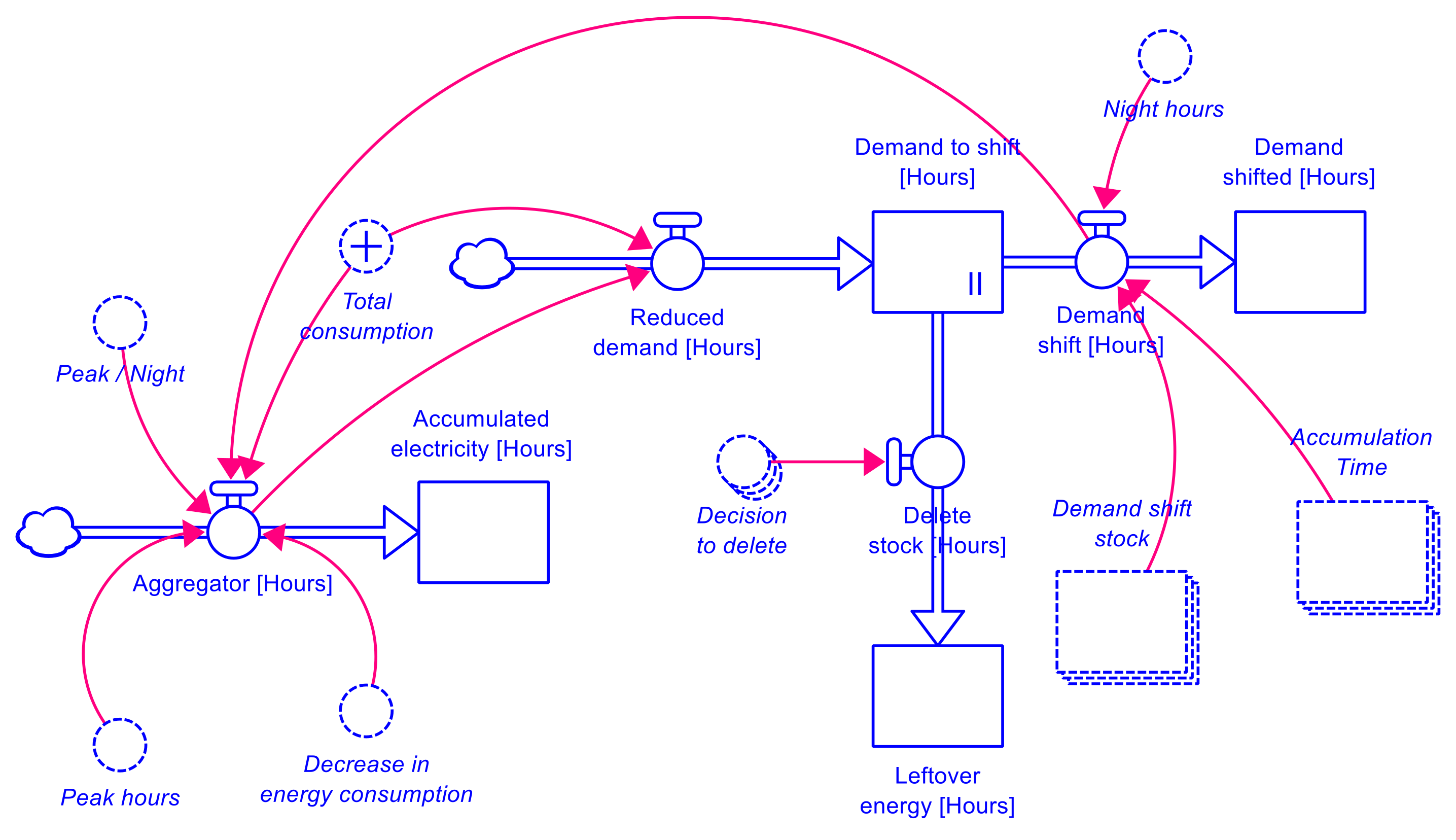
The load aggregator submodel (aggregator hours) has been shown in Figure 9, in which the shifted load has been calculated by considering the hourly power consumption differences and potential for power increase or decrease.

The potential aggregated and shifted power consumption is determined by analysing power consumption in particular periods. In addition, the peak-to-night ratio is introduced to shift electricity from peak hours to night hours in the aggregator (hours) scenario. Finally, the shifted power flow “aggregator (hours)” is determined by calculating the potential aggregated amount of power using the following if function:

$$A_H=if\left(f_P=1; E_{CONS}·\left(1-E_{DECR}\right);E_{CONS}+T_{DS}·f_{P/N}\right)$$

(8)

where A_H—aggregated power for aggregator (Hours), MW; f_P—peak hour rate; E_CONS—power consumption, MW/h; E_DECR—potential power consumption decrease, MW/h; T_DS—potential demand shift, hours; f_PN—peak/night hour ratio;

When the time reaches the night hour value, the reduced electricity consumption is fed into the electricity consumption stream, thus shifting the electricity consumption from peak hours to the night hours:

$$E_{SHIFT}=IF(f_N=1, \frac{E{S}_{SHIFT}}{E_{TIME}}, 0)$$

(9)

where E_SHIFT—demand shift, MW; f_N—night hour factor; ${ES}_{SHIFT}$—accumulated demand; $E_{TIME}$—accumulation time.

The power consumption decrease rate depends on the share of power consumption that can be shifted, expresses what part of the total electricity consumption can be reduced, and the share of aggregator customers. The higher the share of aggregator customers, the more significant reduction of electricity consumption can be achieved. The study assumes that the 10% of total power consumption could be shifted to another period which is determined according to previous studies of several authors [42,43].

$$e_{DECR}=e_{DS}·f_{AC}$$

(10)

where $e_{DS}$—shiftable power consumption rate; $f_{AC}$—share of aggregators’ customers.

The share of aggregators’ customers in the variable and calculated, depending on how much electricity can be reduced and shifted. Two stocks “installed capacity without aggregator service” and “installed capacity with aggregator service” are considered.

$$E_{AGG}={{\displaystyle \int }}_{t0}^t{E}_{AGG}\left(t_0\right)+E_{AGG+}·dt$$

(11)

where $E_{AGG}$—consumption capacity with aggregator service, MW; $E_{AGG+}$—a shift of capacity with aggregator services, MW/Hours.

Exceeding the 50% share of aggregator customers reduces the growth rate because acquiring new customers for the aggregator service is more complicated. In addition, there is a limiting parameter, the “boundary fraction”, which determines how many customers of all can connect to the aggregator service.

In addition to the potential to shift the power demand, there is also an outgoing flow for deleting the shifted power consumption because of the assumption that electricity can only be shifted within 12 h period. Therefore, before the start of the peak hour, the shifted stock is cleared and has a value of zero:

$$E_{SHIFT, DEL}=IF(T_{24\mathrm{h}}>T_{N,END}, INF, 0)$$

(12)

where E_DEL—Deleted shifted power consumption, MW; T_24h—Modelling time described in 24 h period, h; $T_{N,END}$—end of night hours, h.

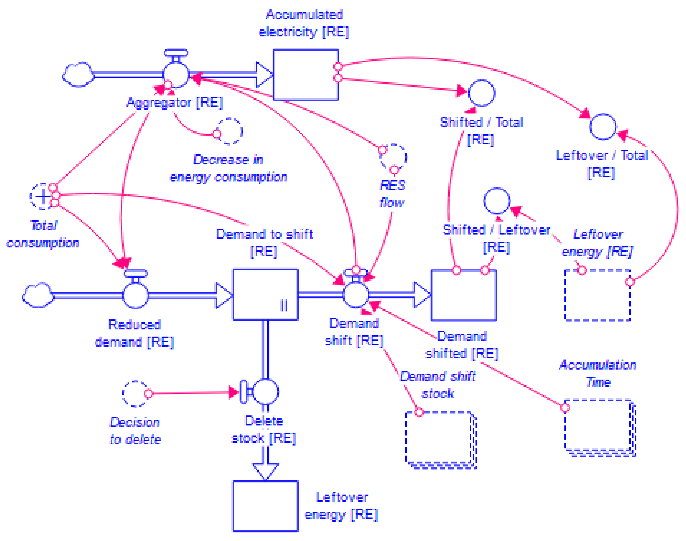
The flexibility aggregator sub-model (aggregator RES) has a similar operating structure as the aggregator (hours) sub-model (see Figure 10).

The main difference is that the power load is shifted based on the available RES energy flow or how much electricity was produced from RES each hour. Therefore, when the amount of RES produced is higher than the electricity consumption, the electricity consumption is increased by the same rate as the power reduction rate described previously:

$$A_{RES}=if\left(E_{RES}>E_{CONS}; E_{CONS}·\left(1+E_{INCR}\right);E_{CONS}-T_{DS}·f_{P/N}\right)$$

(13)

where A_RES—aggregated power for aggregator (RES), MW; E_RES—RES power production, MW/h; $E_{INCR}$—power increase rate, MW/h.

2.5. Combining Production and Demand-Side, Surplus Calculation

The last part of the modelling is to compare production and consumption sub-models to evaluate the effect of different renewable capacities and demand-side management options on surplus energy from renewable energy sources.

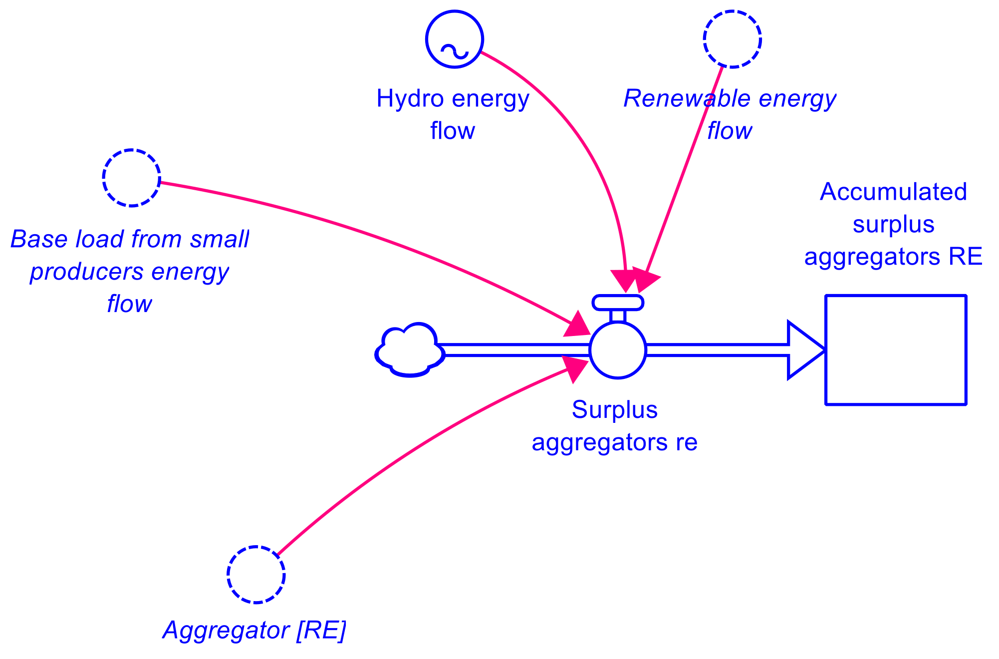
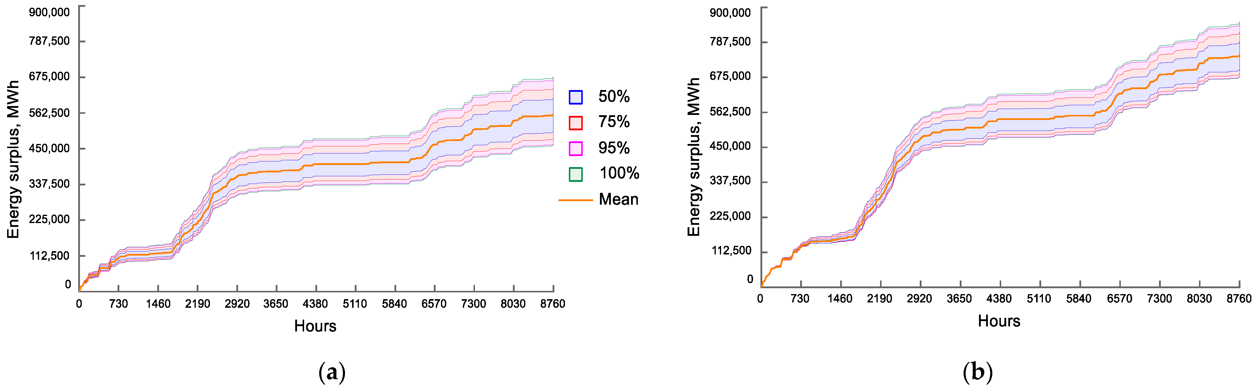
In Figure 11, the hourly production amount is compared to consumption in case of shifting the load based on RES availability, but the same structure is also used for calculating the energy surplus when the load-shifting based on demand is in place. The hourly flow of surplus is calculated based on the following equation:

$$IF(\left(E_{RES}+E_{HES}+E_{Base}-E_{CONS}\right)>0;E_{RES}+E_{HES}+E_{Base}-E_{CONS};0)$$

(14)

where E_HES—hourly hydro energy production, MWh/hour; E_Base—hourly baseload from small producers, MWh/hour. The accumulated energy surplus for a specific period is calculated based on Equation (7).

3. Results

The section presents the main hourly and annual results regarding RES power production and possible surplus power reduction through aggregator introduction.

RES Power Production

As described in Section 2.2, 4 different power capacities of variable RES (VRES) combinations were analysed. Figure 12 presents the annual accumulated power production rate for different installed VRE capacities based on the previously built SD model to forecast the future trends of RES technologies installation. Scenario 1 shows the existing situation without solar electricity production and a small amount of wind power, which reaches only 160 MWh. In Scenario 2, when installed solar plant capacity reaches 100 MW, but the capacity of wind farms is 500 MW, the total solar power production is almost 100 MWh per year, but accumulated wind power reaches 1042 MWh per year. This amount is almost doubled in Scenario 3 with additional support policies for wind and solar plants, with total accumulated solar power of 148 MWh and 2008 MWh of wind power. Finally, the increase of solar power production rates is simulated in Scenario 4 when installed solar power capacity reaches 964 MW and produces 948 MWh per year, but the wind power plants provide only 310 MWh of electricity.

The hourly power production in each scenario can be seen in Figure 13. The production includes the hydropower plants with a nominal capacity of 1000 MW and the baseload provided by biomass cogeneration plants (30 MW) to present the national energy balance accurately. Thus, hydro generation hourly and baseload profiles are constant in all scenarios, and only solar and wind profiles change based on installed capacities.

As shown in Figure 13, most of the power in Scenario 1 and Scenario 2 is produced by hydropower, but in Scenario 3 significant additional amount is provided by installed wind turbines. In Scenario 4, a high share of power is produced during the late spring and summer periods when there is higher solar irradiation due to the high capacity of installed solar power plants. Further, the hourly production rates are compared with the power consumption to estimate the surplus VRE electricity amounts.

In Figure 14, the ratio between power production and consumption are displayed. When the ratio is 1, the production rate for a particular hour is equal to consumption. However, when the ratio exceeds 1, the production rate is higher than the consumption rate. In Scenario 1, there are only a few hours when production exceeds consumption, but in Scenario 2 and 3, the ratio exceeds 1 significantly more due to the higher wind capacities. Scenario 4 also shows improvement in production and consumption ratio. However, it is not as significant as in Scenario 3. Although Scenario 4 used the same capacity for PV panels as for wind in Scenario 3, less energy is generated due to lower energy conversion efficiency for PV panels. In addition, PV technologies are significantly affected by seasonality and weather conditions.

When the ratio exceeds 1 and production is higher than consumption, surplus power occurs. Based on the hourly graphs displayed in Figure 14, the total amount of accumulated surplus power can be calculated. In Figure 15, the accumulated surplus is displayed to measure the amount of energy that can be redirected or exported over the year. Scenario 3 shows the highest amount of surplus VRE power—over 600,000 MWh per year.

In Figure 16, the different perspective of surplus energy is revealed. In the case of low installed capacity, only a small amount of surplus power occurs. For example, in Scenario 1, only around 6 % of total electricity produced from RES (excluding hydro energy) cannot be consumed immediately. However, in Scenario 3, this number increases to 30% from total energy produced from RES. These results are in line with similar previous research. Andresen et al. [44] have analysed the impact on high shares of installed wind and solar power capacities. In the case of 100% of wind power scenario, 30% of surplus power occurs. However, the surplus power for low solar and wind capacities are insignificant.

Aggregators and potential load shifts have been introduced to decrease the amount of occurred surplus power. As described in Section 2.3, two types of aggregators have been tested. The aggregator (hours) smoothens the power consumption load by shifting the peak consumption to off-peak hours during the night while the aggregator (RES) shifts the power consumption load to the hours with higher VRE power production hours. The example of power consumption changes as a result of introducing two different aggregator types has been shown in Figure 17. The graph shows the total hourly RES production and total power consumption for two weeks in March. As seen in the case of the aggregator (RES) introduction, the power consumption is shifted to the periods when there are higher solar and wind power production rates. On the contrary, when the aggregator (hours) is operating, the peak power consumption is reduced but does not follow the RES production rates.

The results also depend on the total share of consumers with aggregator services. Therefore, several shares of connected consumers have been tested in Figure 14. The percentages represent the diffusion level of aggregators in the system. For example, 0% means that no consumer is using the service of aggregators. However, 100 % means that all consumers who are eligible use the service of aggregators. From Figure 18, when load shift is introduced according to available RES power, the surplus power can be eliminated in Scenario 1. In Scenarios 3, surplus power reduces from 30% to 24% when all consumers shift their power load with the help of aggregator services. However, the surplus power amount increases when shifting load from peak hours to off-peak hours and not considering the RES energy availability. The highest increase from 6% to 23% is seen in Scenario 1 when few wind capacities are installed. In Scenario 3, the surplus power could increase by 3% if the power load is smoothed. On the other hand, the smoothened power load can benefit from decreased installed capacities and primary energy savings when operating in baseload conditions. Further investigation could be performed to compare the obtained costs and savings from the economic perspective.

The sensitivity analyses have been performed to analyse the impact of the main variable on the obtained results. As can be seen in Figure 19, the changes of shiftable load can either increase or decrease the obtained results of surplus power. For example, if the assumed shiftable load is increased from 10% to 20%, which could be the case if the most significant power consumers adjust their power consumption and increase the flexibility, the aggregator (RES) can decrease the surplus power by 16% in case of high wind share scenario (Scenario 3). On the other hand, the opposite situation occurs in the case of the aggregator (hours) scenario, which could significantly (by 22%) increase the surplus power from VRES if the share of shiftable loads increases.

4. Discussion

This section discusses the limitations of the results, the methods and materials, and the assumptions made for the analyses. The results presented in this paper indicate that power balancing issues due to large shares of VRE in power generation mixes could be decreased and, to some extent, prevented by the possible load shift and integration of aggregators as a market player. Therefore, the results should be considered applicable for the national scale analyses where different power consumers and additional power loads are present. Even though there are other possibilities to utilise the occurred surplus power from VRES, such as the power-to-x concept, power and heat accumulation systems, in-depth analyses are performed for the impact of power load flexibility analyses. However, further studies could compare different scenarios for surplus power utilisation by determining the cost-effectiveness and overall impact on reached renewable power shares.

A limitation of this study is that it has a technical approach and does not consider economic or policy aspects that might influence the system performance. The introduction of aggregators previously is mainly highlighted from the economic perspective. It is associated with power cost reduction potential when power consumption is increased in low power price periods. However, the preliminary analyses on historical market prices of electricity did not show the relation with the increased penetration of VRES due to relatively low market shares of wind and solar power electricity in the Baltic states. Therefore, different load shift mechanisms were introduced without focusing on hourly market prices. The particular article analyses the benefits from higher renewable power utilisation perceptive.

The obtained results on surplus power and shiftable loads are highly dependent on the modelled power capacities, added base loads, and power consumption patterns. Therefore, even though the presented methodology can be applied to other countries, the results can differ for countries without significant hydropower or biomass cogeneration as baseload.

Also, the power consumption patterns could be different for countries with significant power-intensive industries, which is not the case in Latvia. Furthermore, power loads might vary between years due to differences in average outdoor temperatures or changes in consumer habits. For example, working from home increases power consumption in households and reduces the consumption in office buildings in different periods. However, as the study includes different types of consumers (by size, type and location), the average consumption patterns are valid for the detailed analyses.

The power demand and solar and wind generation used in the calculations represent data for 2018. It means that the VRE production profile and, thus, the power balancing profile reflected the wind and solar power generation conditions in 2018. The power generation will differ between years due to varying weather conditions—hourly solar irradiation and wind speed. Also, the balancing load of hydropower is based on the data from the year 2018. However, there are variations in a hydrologic regime each year which reflects the produced hydropower. Therefore, the surplus power can slightly change year by year due to several climatic conditions.

5. Conclusions

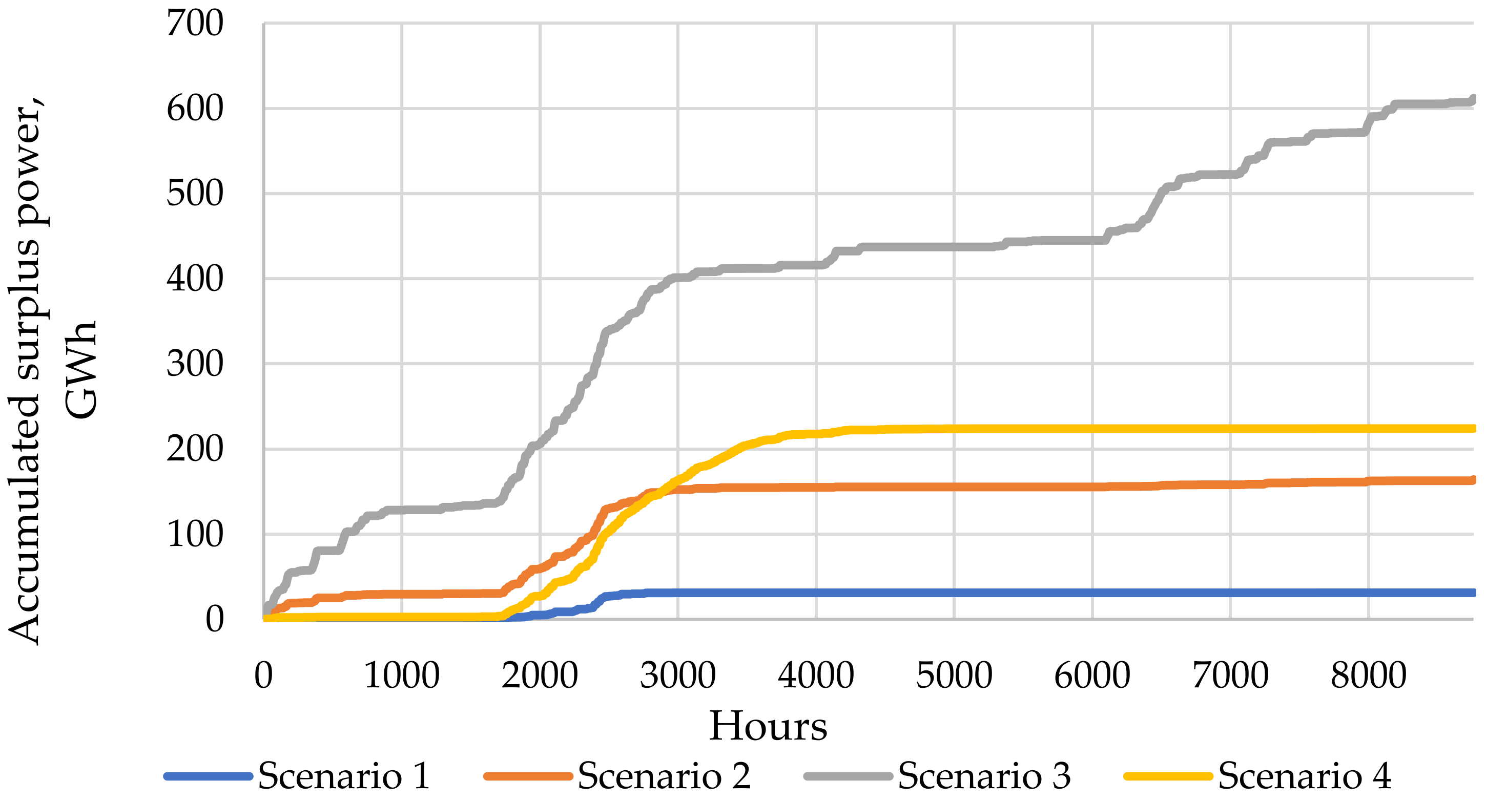
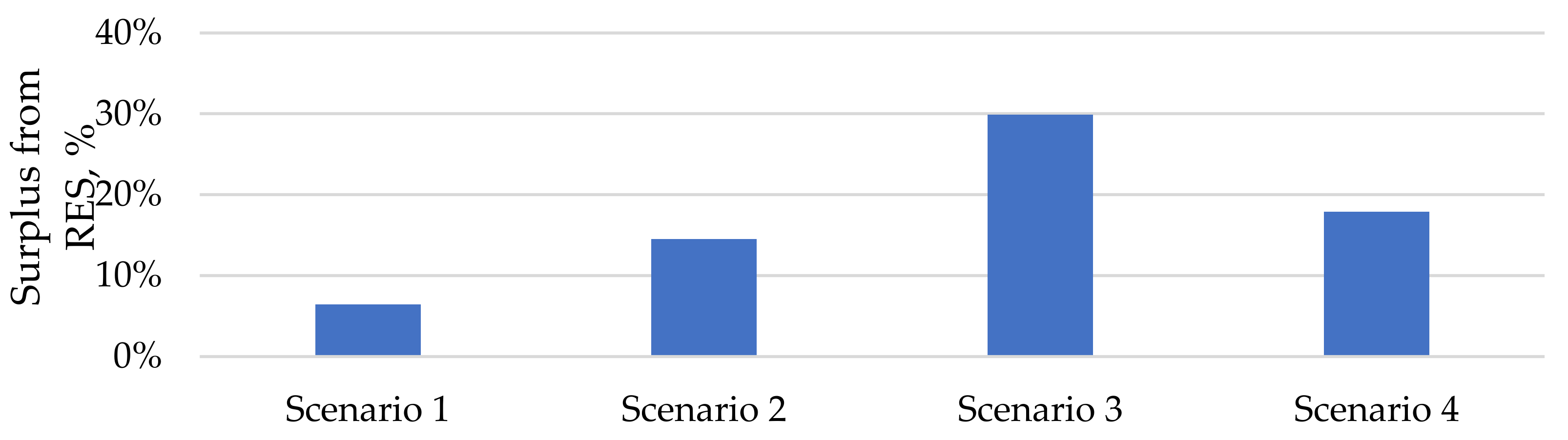
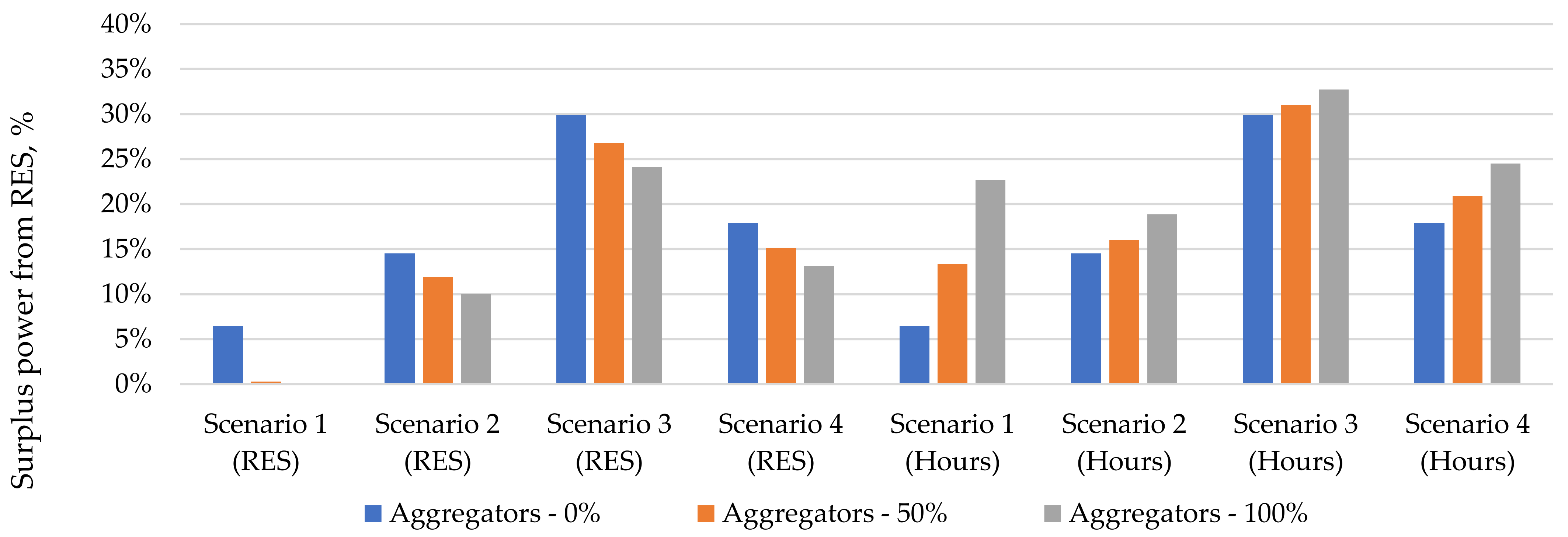
The research analyses the potential impacts of demand-side management on the utilised power from RES—solar and wind power plants. The system dynamics modelling merges the forecasted variable power capacities from the national scale forecasting model with the hourly solar and wind production profiles. The results show that when there are large installed wind capacities, around 30% of the generated power occurs in periods without sufficient demand profile, and surplus power occurs.

The results show that the utilised VRE power share does not increase when introducing aggregator, which shifts the peak demand to off-peak periods. On the contrary, the demand shift results in higher power surpluses. However, when the load shift follows the RES power production rates, the surplus power can be reduced by around 5%. However, in this case, all consumers should have participated in the demand shift and have an aggregator service, which would probably not be feasible in reality.

The proposed methodology can be applied and tested internationally to evaluate the future perspectives of flexible power production and consumption in countries with similar power market structures, for example, Baltic and Scandinavian countries. Obtained results can be further used in other energy policy testing and as a support for the definition of the legislative framework of aggregators. Results show that their future role should also focus on renewable share increase, providing financial benefits from shifting demand to lower electricity price periods.

The presented research will be continued by analysing the economic and environmental benefits of demand-side management and load shifting. Furthermore, the model allows testing different policy frameworks, which could be further investigated for the successful performance of aggregators towards carbon-neutral energy production.