Frequency Regulation System: A Deep Learning Identification, Type-3 Fuzzy Control and LMI Stability Analysis


 ,
, 
 and
and 
Abstract
:
1. Introduction
- The dynamics of all units in all areas are considered to be unknown;
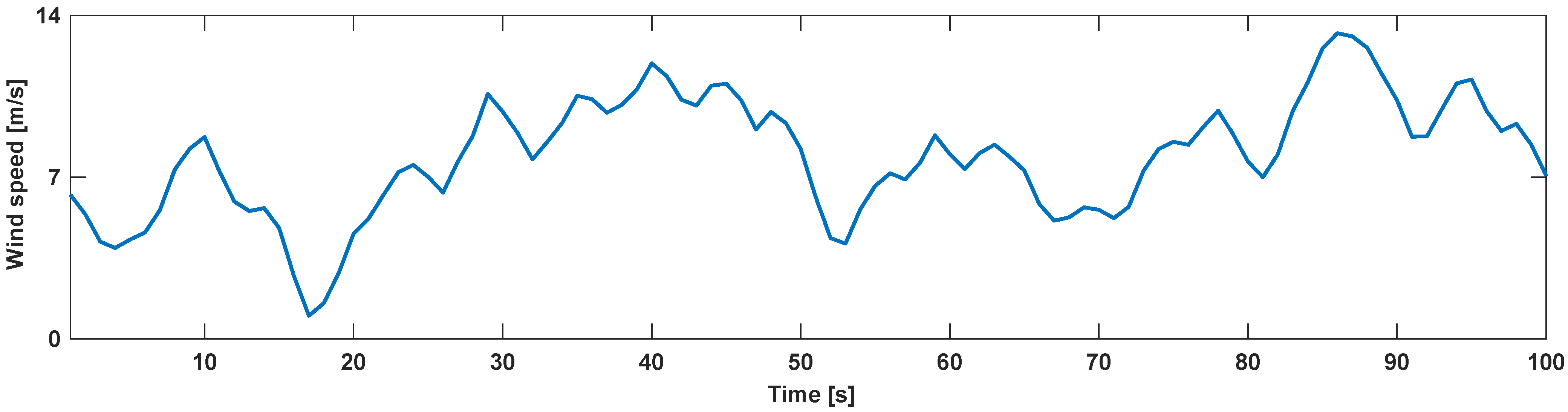
- In addition to unknown dynamics, the effects of time-varying parameters, solar radiation, wind speed, and multiple load changes are taken to account;
- A novel dynamic fractional-order model using RBMs and deep learning algorithm is proposed for online identification;
- A novel compensator on basis of IT3-FLS is presented to cope with the dynamic model approximation error;
- A new LMI approach is developed to derive the error feedback gains and to guarantee the stability and robustness.
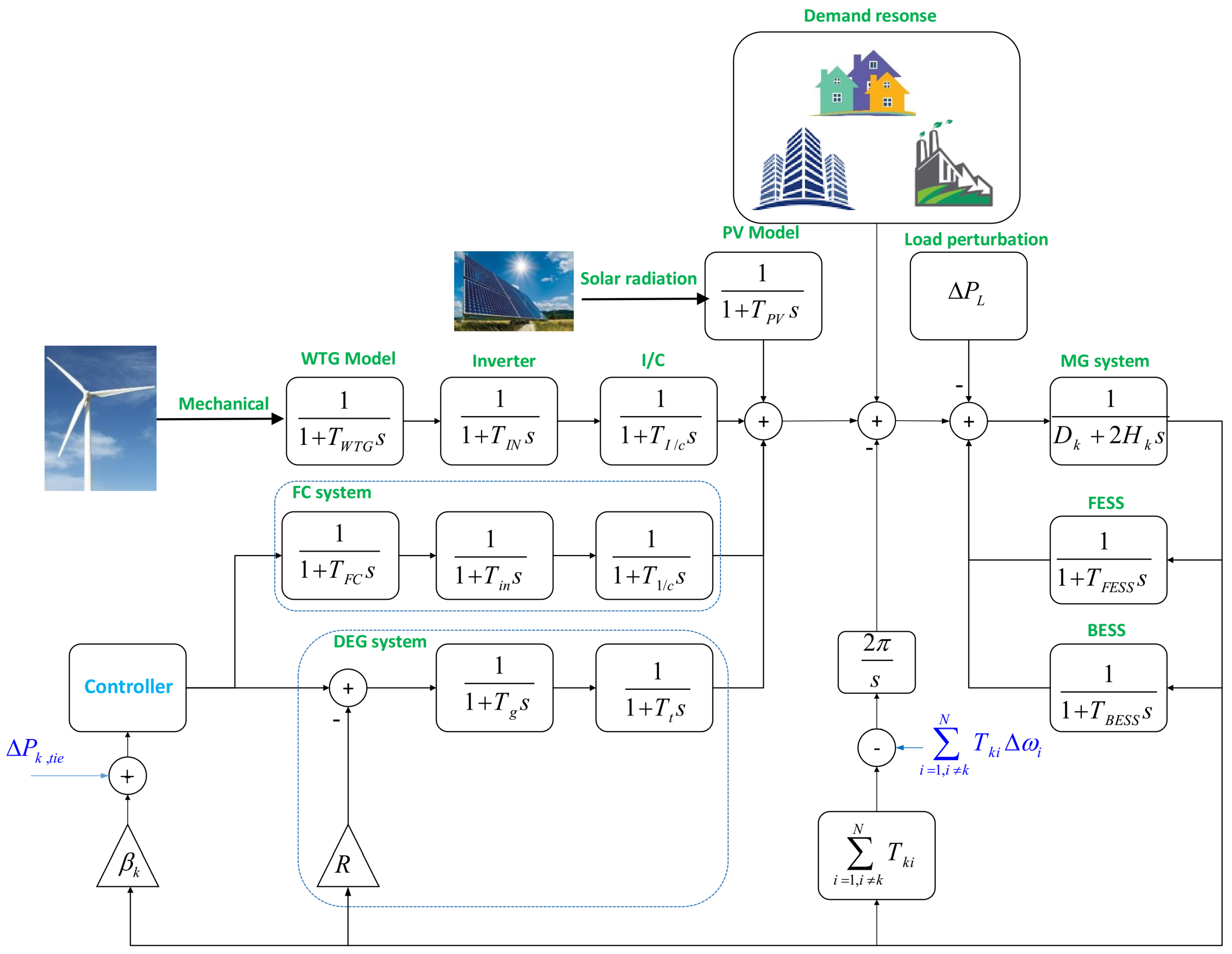
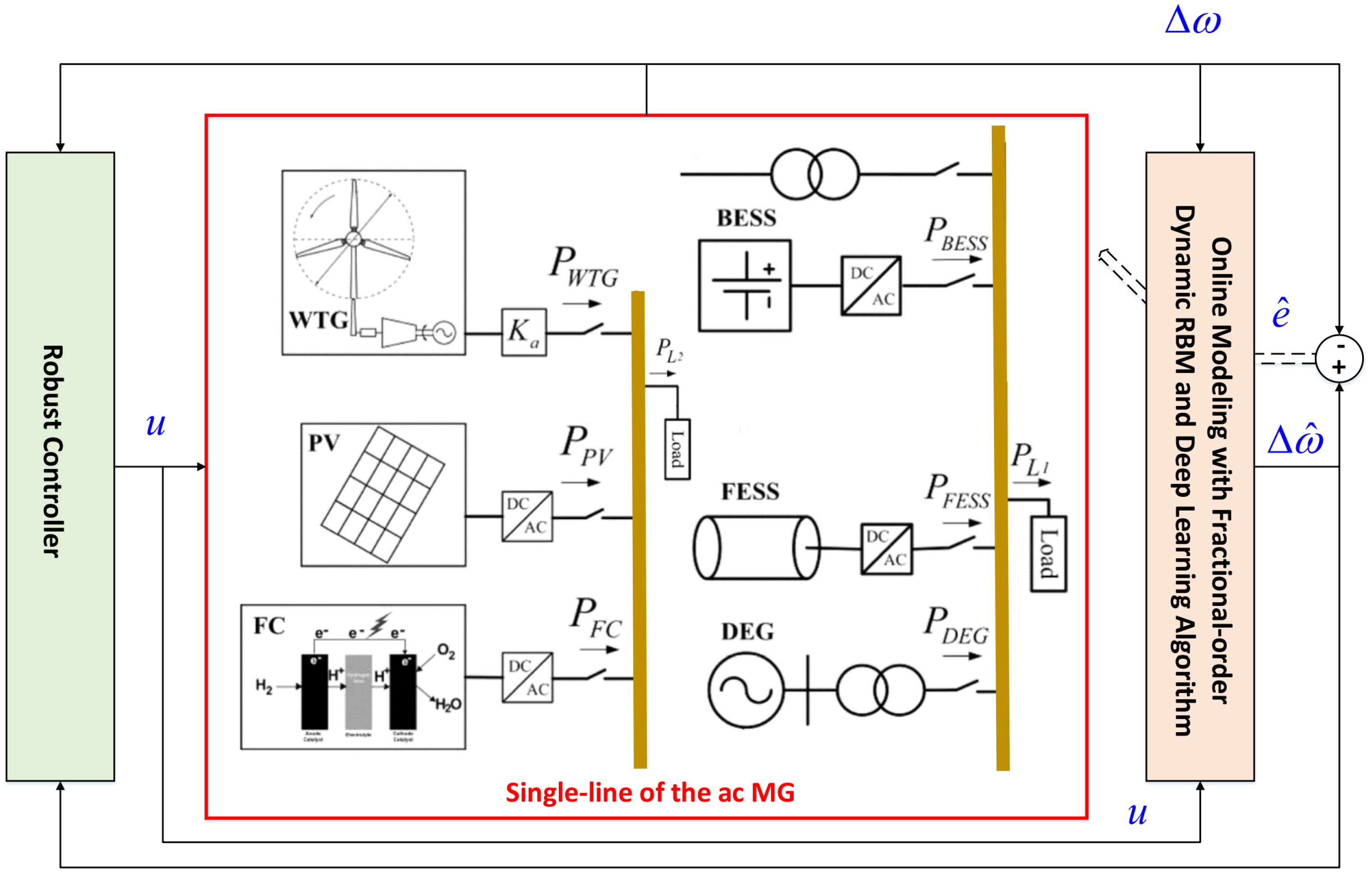
2. System Description
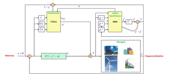
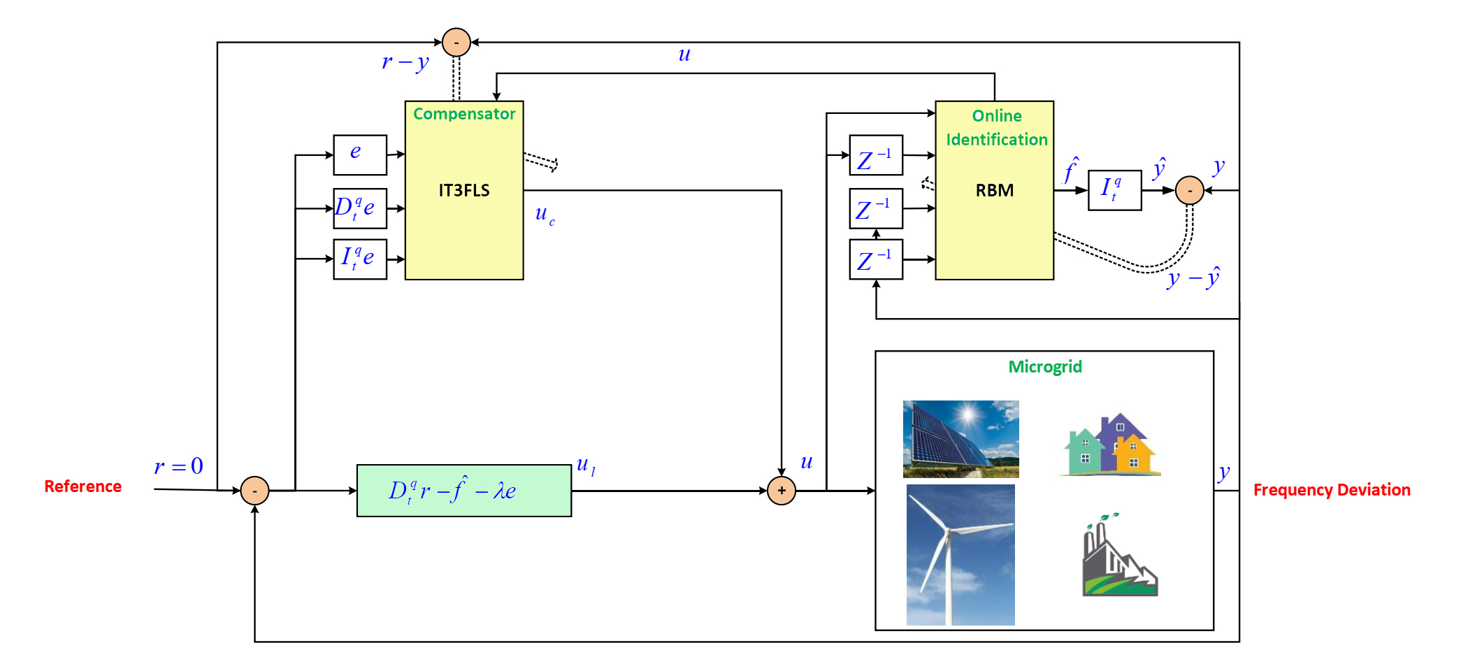
3. A General View on Presented Control System
4. Proposed Dynamic Fractional-Order Model
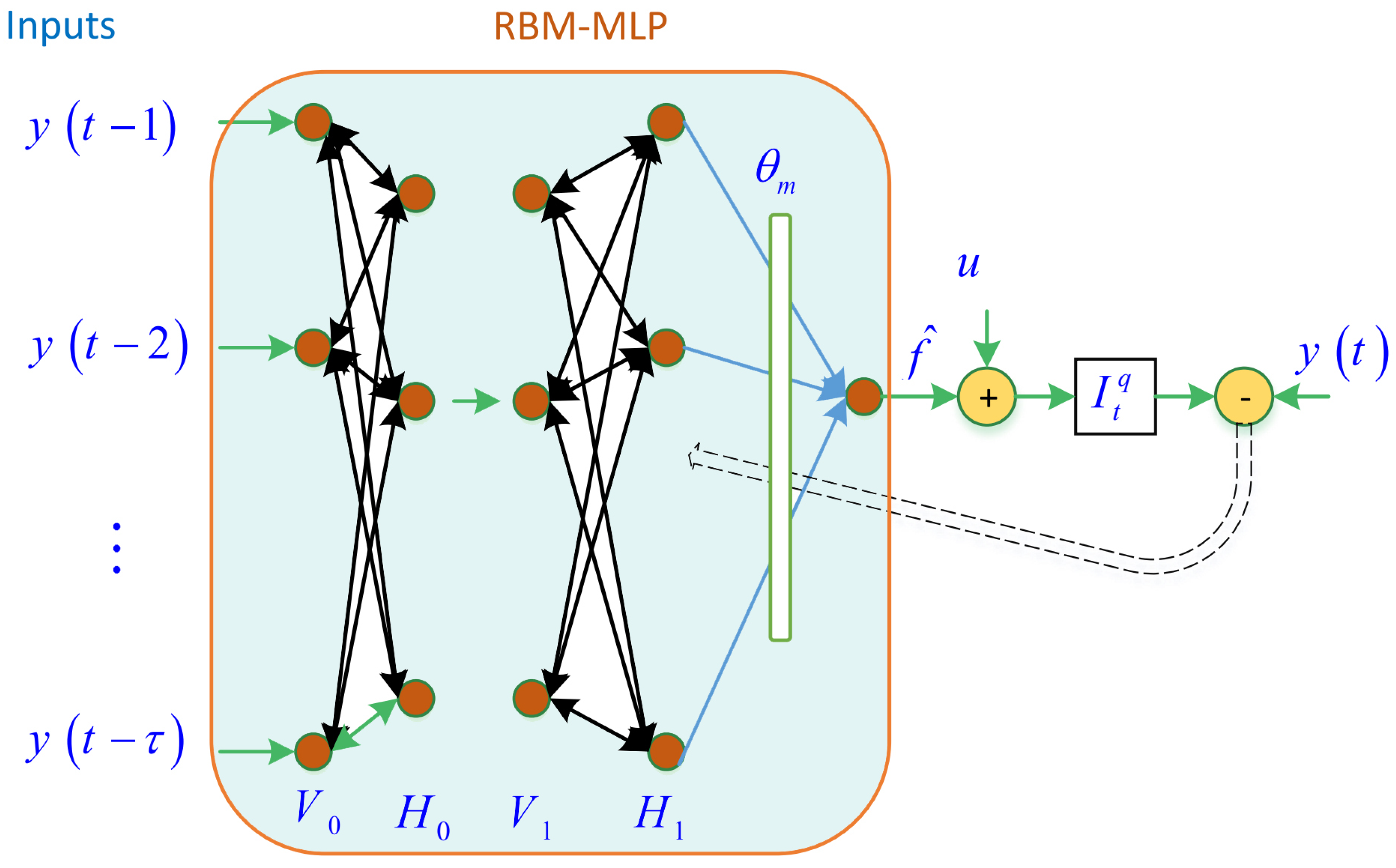
4.1. Structure
- (1)
- The inputs of RBM-MLP are the outputs of the system at the previous sample times;
- (2)
- The inputs are considered as the visible nodes and the outputs in the hidden layer are obtained as:where, is a matrix, is the number of inputs, n is the number of neurons, is vector and ;
- (3)
- From , the vector is obtained as:where, that is obtained in the previous step is vector and is a vector;
- (4)
- Similarly form the vector is obtained as:where, is a vector;
- (5)
- Finally the output is obtained as:where, represents the fractional integral, is the control signal in the k-th area and is vector.
4.2. Learning
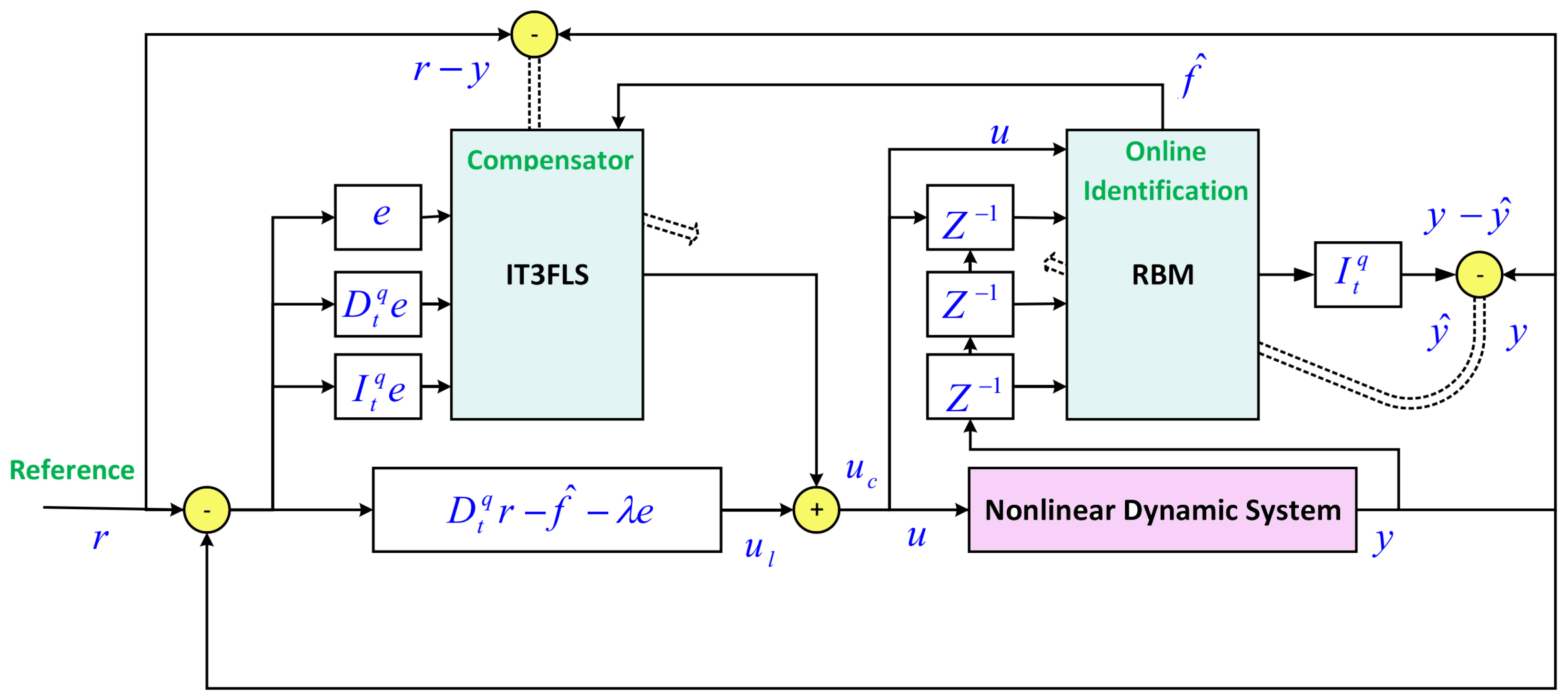
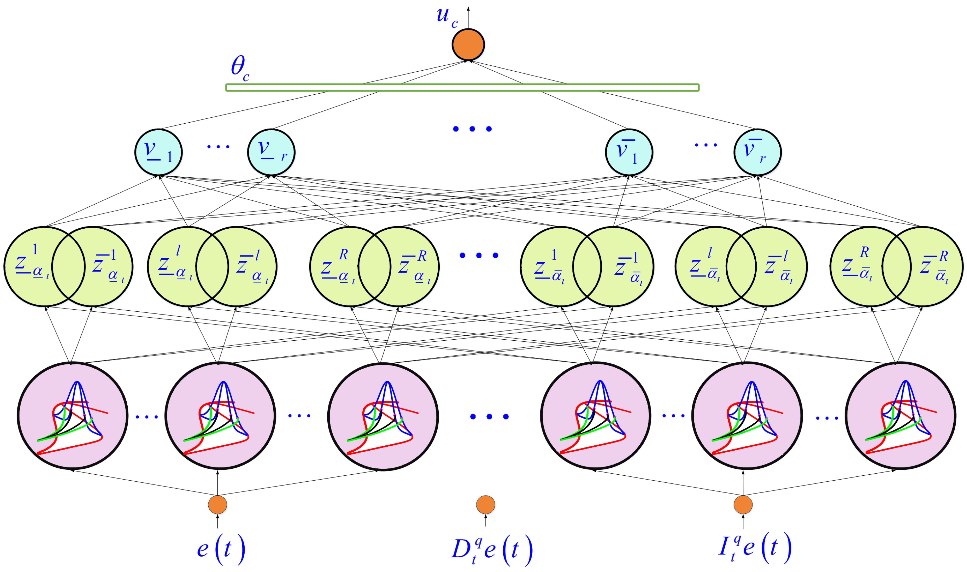
5. Proposed Type-3 Fuzzy Compensator
5.1. Structure
- (1)
- The inputs are , and , where, and represent the stabilization error, fractional derivative and integral of stabilization error, respectively;
- (2)
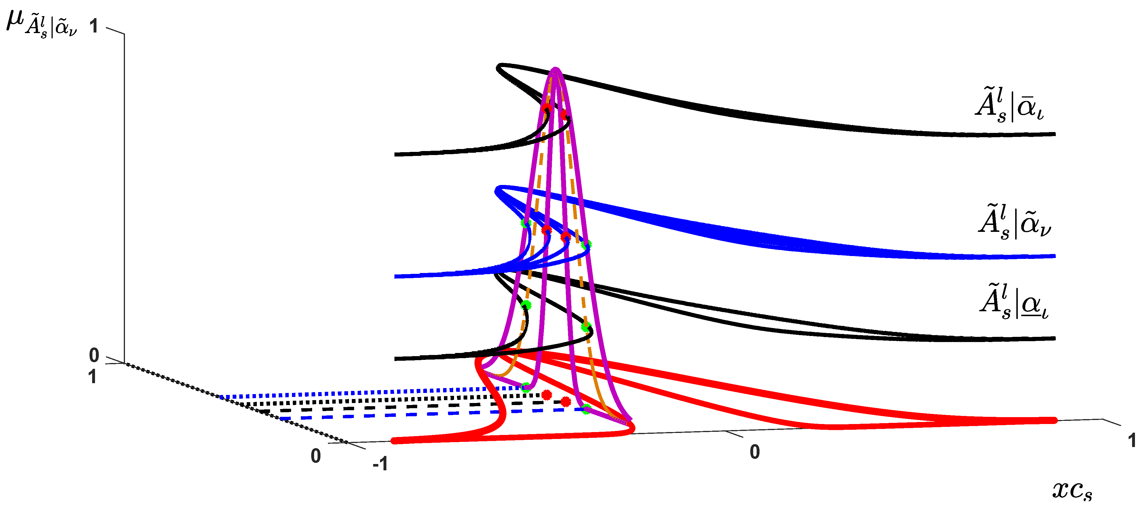
- For each inputs , and , R membership functions (MFs) are considered as , , with r slices (). Then for input , one has:where, is the center of Gaussian MF , and are the upper standard division of at and levels, respectively, and and are the lower standard division of at slice level and , respectively (see Figure 6);
- (3)
- For each MFs in the step 2, one rule is considered. Then the number of rules is R and rule firings are:
- (4)
- By type-reduction in [37], the output of compensator is concluded as:where,where, and are the upper and lower l-th rule parameters. The vector of rule parameters is:
5.2. Learning
6. Stability Analysis
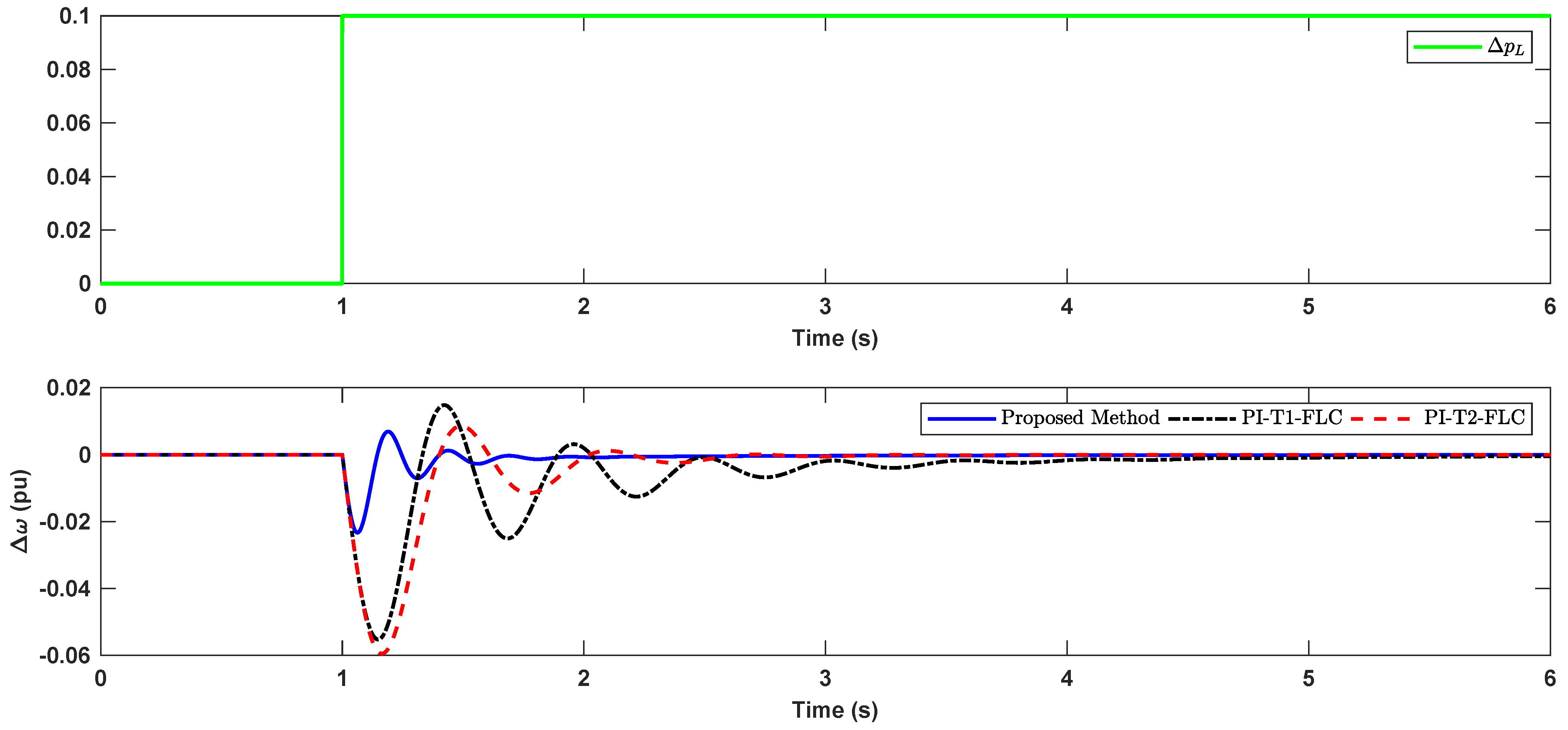
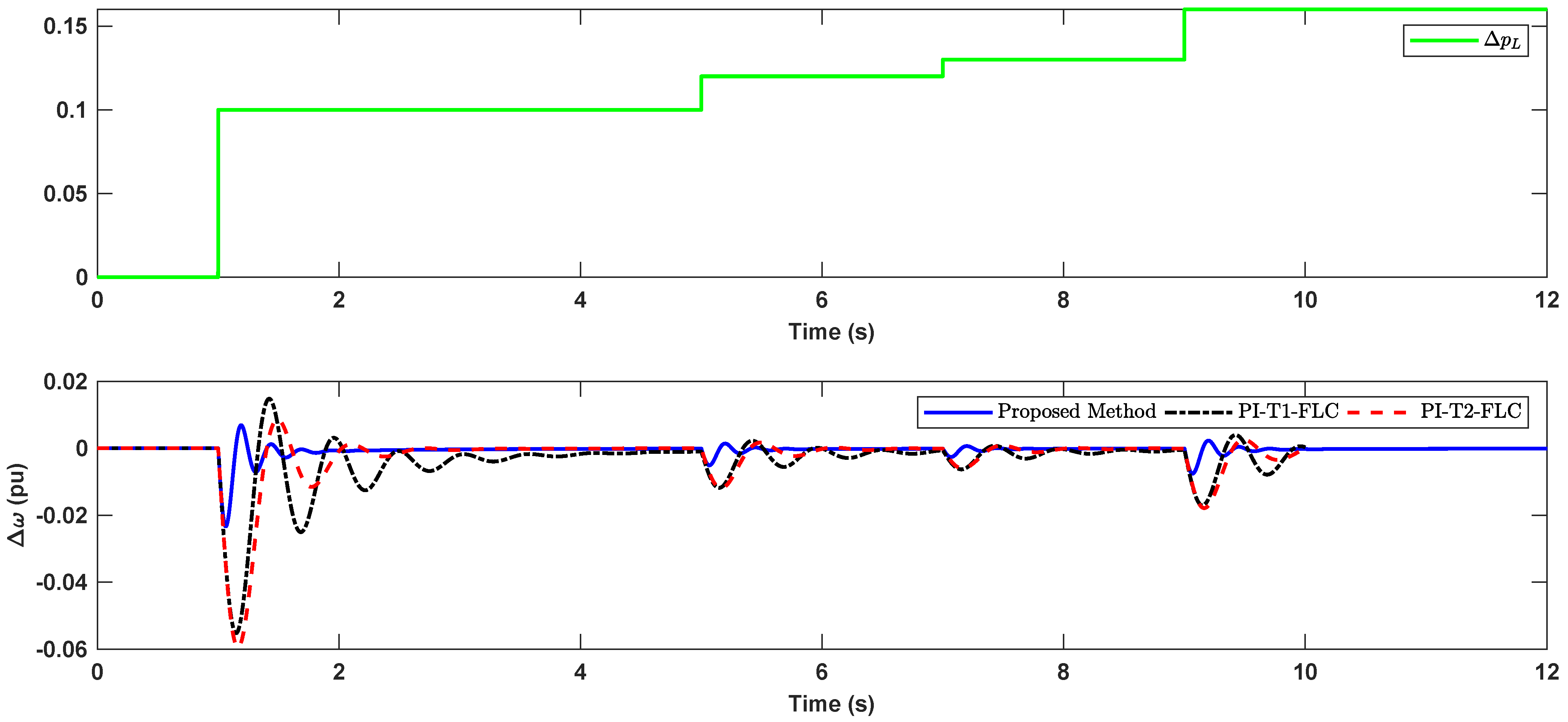
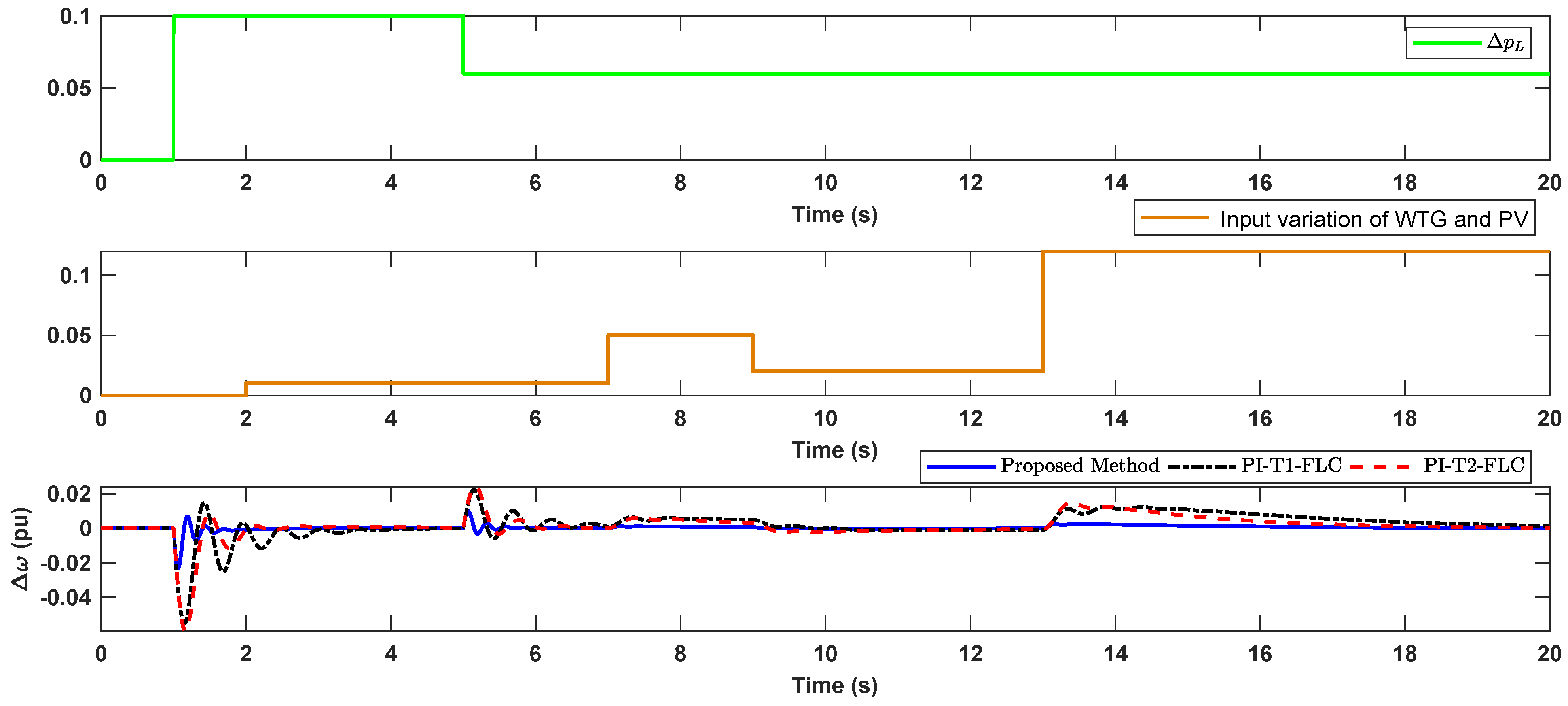
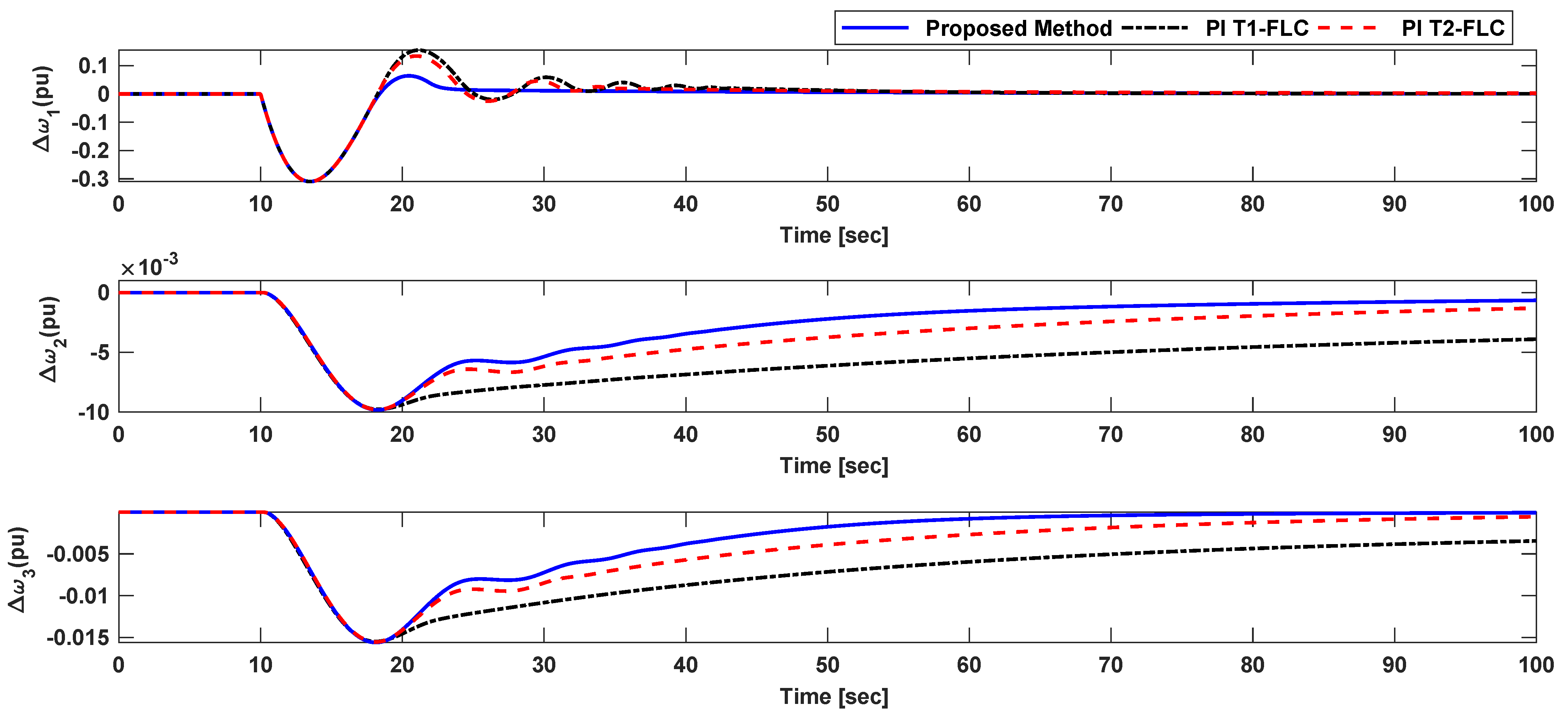
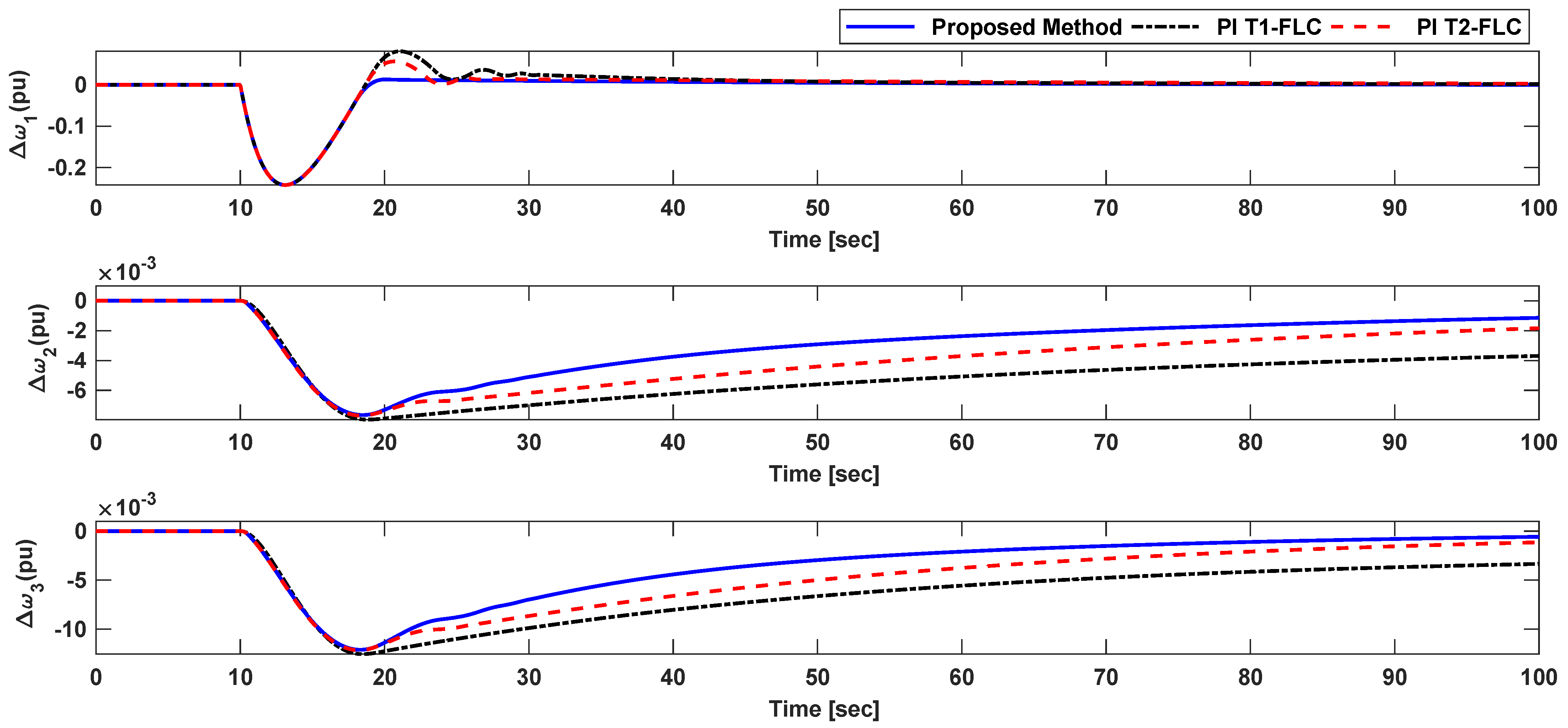
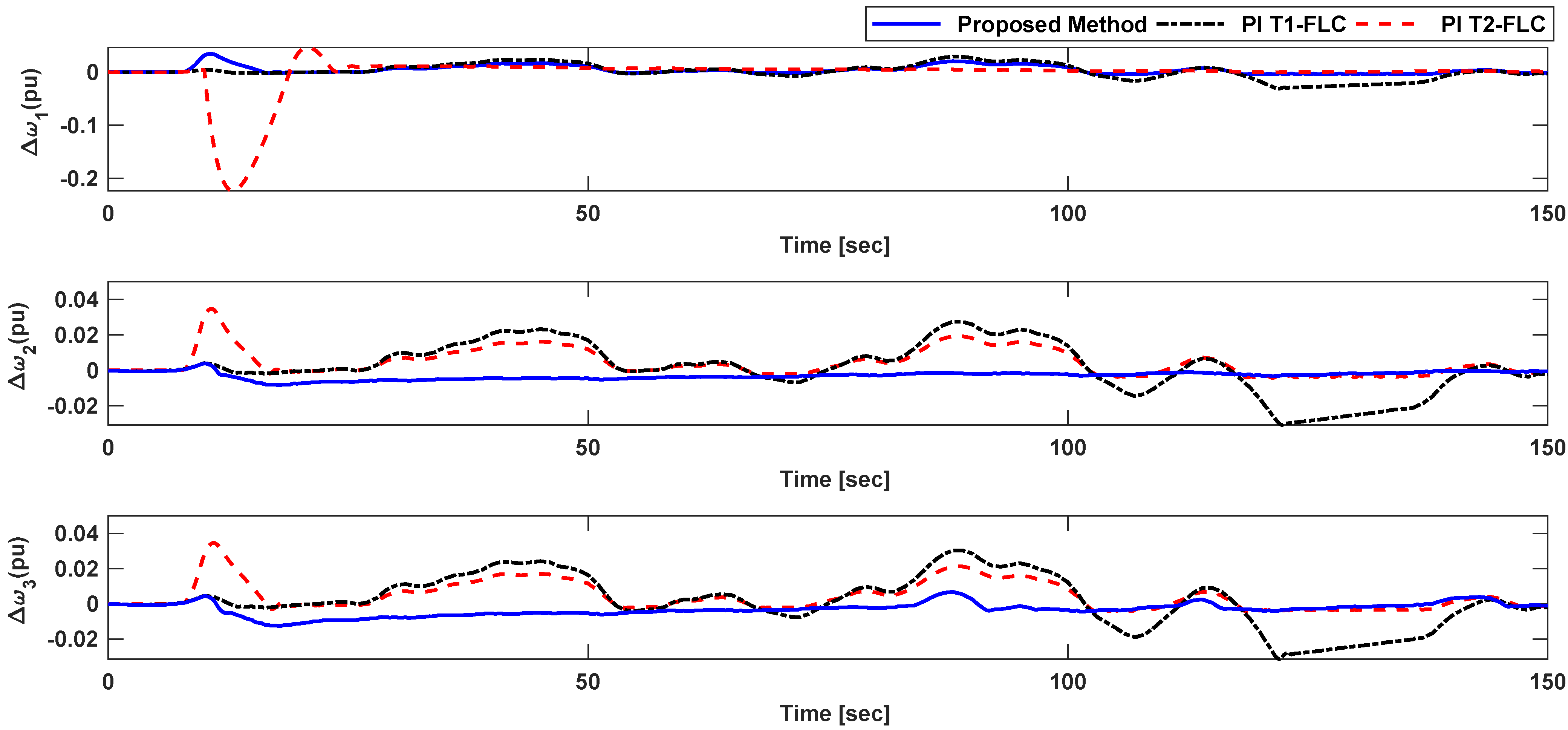
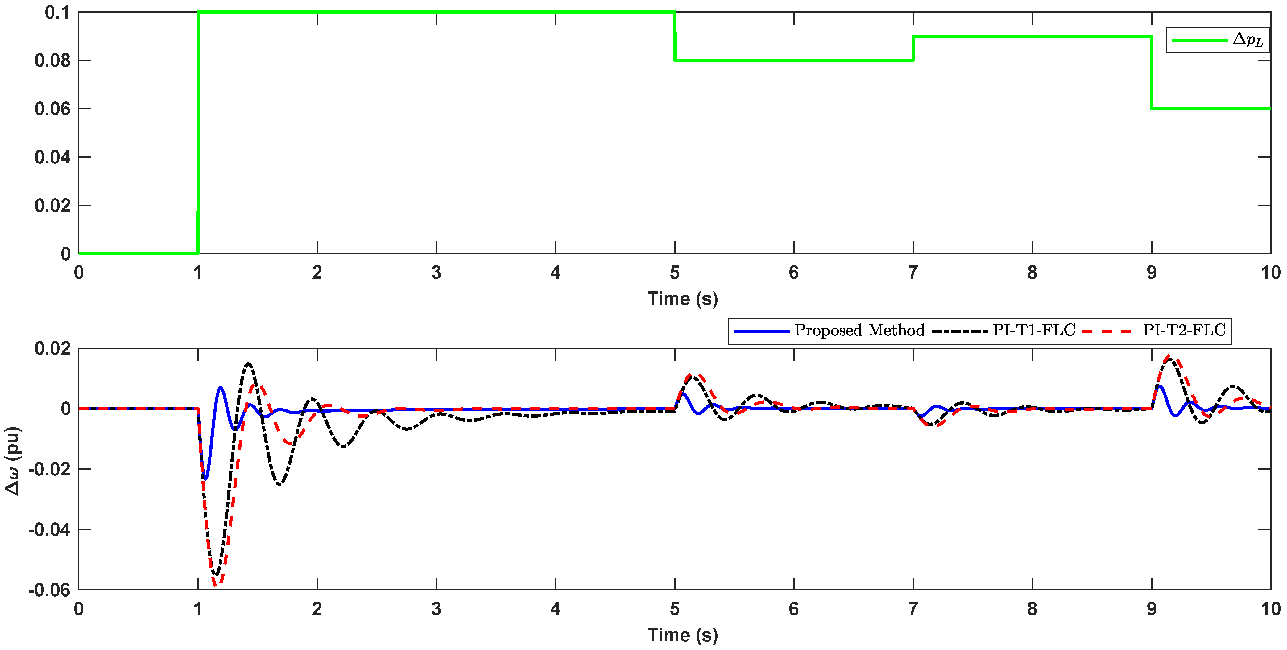
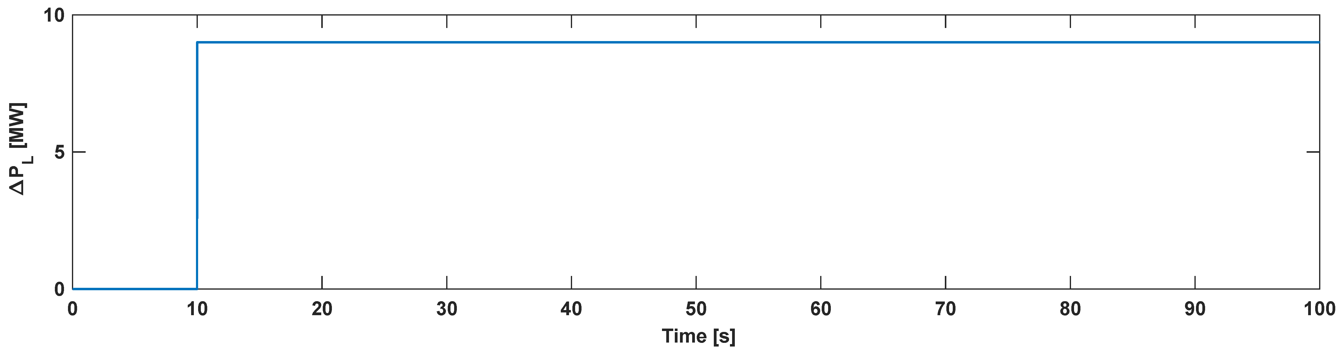
7. Simulation
8. Conclusions
Author Contributions
Funding
Institutional Review Board Statement
Informed Consent Statement
Data Availability Statement
Acknowledgments
Conflicts of Interest
Appendix A. Stability Analysis
References
- Mihet-Popa, L.; Saponara, S. Power Converters, Electric Drives and Energy Storage Systems for Electrified Transportation and Smart Grid Applications. Energies 2021, 14, 4142. [Google Scholar] [CrossRef]
- Subramanian, S.; Sankaralingam, C.; Elavarasan, R.M.; Vijayaraghavan, R.R.; Raju, K.; Mihet-Popa, L. An Evaluation on Wind Energy Potential Using Multi-Objective Optimization Based Non-Dominated Sorting Genetic Algorithm III. Sustainability 2021, 13, 410. [Google Scholar] [CrossRef]
- Armghan, A.; Azeem, M.K.; Armghan, H.; Yang, M.; Alenezi, F.; Hassan, M. Dynamical Operation Based Robust Nonlinear Control of DC Microgrid Considering Renewable Energy Integration. Energies 2021, 14, 3988. [Google Scholar] [CrossRef]
- Marti-Puig, P.; Blanco-M, A.; Cárdenas, J.J.; Cusidó, J.; Solé-Casals, J. Feature selection algorithms for wind turbine failure prediction. Energies 2019, 12, 453. [Google Scholar] [CrossRef] [Green Version]
- Armghan, A.; Hassan, M.; Armghan, H.; Yang, M.; Alenezi, F.; Azeem, M.K.; Ali, N. Barrier Function Based Adaptive Sliding Mode Controller for a Hybrid AC/DC Microgrid Involving Multiple Renewables. Appl. Sci. 2021, 11, 8672. [Google Scholar] [CrossRef]
- Shabani, H.; Vahidi, B.; Ebrahimpour, M. A robust PID controller based on imperialist competitive algorithm for load-frequency control of power systems. ISA Trans. 2013, 52, 88–95. [Google Scholar] [CrossRef]
- Farahani, M.; Ganjefar, S.; Alizadeh, M. PID controller adjustment using chaotic optimisation algorithm for multi-area load frequency control. IET Control Theory Appl. 2012, 6, 1984–1992. [Google Scholar] [CrossRef]
- Wies, R.W.; Chukkapalli, E.; Mueller-Stoffels, M. Improved frequency regulation in mini-grids with high wind contribution using online genetic algorithm for PID tuning. In Proceedings of the 2014 IEEE PES General Meeting|Conference & Exposition, IEEE, New York, NY, USA, 27–31 July 2014; pp. 1–5. [Google Scholar]
- Sahoo, B.; Panda, S. Improved grey wolf optimization technique for fuzzy aided PID controller design for power system frequency control. Sustain. Energy Grids Netw. 2018, 16, 278–299. [Google Scholar] [CrossRef]
- Abedinia, O.; Naderi, M.S.; Ghasemi, A. Robust LFC in deregulated environment: Fuzzy PID using HBMO. In Proceedings of the 2011 10th International Conference on Environment and Electrical Engineering, IEEE, New York, NY, USA, 8–11 May 2011; pp. 1–4. [Google Scholar]
- Ali, E.; Abd-Elazim, S. BFOA based design of PID controller for two area load frequency control with nonlinearities. Int. J. Electr. Power Energy Syst. 2013, 51, 224–231. [Google Scholar] [CrossRef]
- Kouba, N.E.Y.; Menaa, M.; Hasni, M.; Boudour, M. LFC enhancement concerning large wind power integration using new optimised PID controller and RFBs. IET Gener. Transm. Distrib. 2016, 10, 4065–4077. [Google Scholar] [CrossRef]
- Kontogiannis, D.; Bargiotas, D.; Daskalopulu, A. Fuzzy control system for smart energy management in residential buildings based on environmental data. Energies 2021, 14, 752. [Google Scholar] [CrossRef]
- Kontogiannis, D.; Bargiotas, D.; Daskalopulu, A. Minutely active power forecasting models using neural networks. Sustainability 2020, 12, 3177. [Google Scholar] [CrossRef] [Green Version]
- Cusidó, J.; López, A.; Beretta, M. Fault-Tolerant Control of a Wind Turbine Generator Based on Fuzzy Logic and Using Ensemble Learning. Energies 2021, 14, 5167. [Google Scholar] [CrossRef]
- Yesil, E. Interval type-2 fuzzy PID load frequency controller using Big Bang–Big Crunch optimization. Appl. Soft Comput. 2014, 15, 100–112. [Google Scholar] [CrossRef]
- Khooban, M.H.; Niknam, T. A new intelligent online fuzzy tuning approach for multi-area load frequency control: Self Adaptive Modified Bat Algorithm. Int. J. Electr. Power Energy Syst. 2015, 71, 254–261. [Google Scholar] [CrossRef]
- Sahu, B.K.; Pati, S.; Mohanty, P.K.; Panda, S. Teaching–learning based optimization algorithm based fuzzy-PID controller for automatic generation control of multi-area power system. Appl. Soft Comput. 2015, 27, 240–249. [Google Scholar] [CrossRef]
- Gheisarnejad, M. An effective hybrid harmony search and cuckoo optimization algorithm based fuzzy PID controller for load frequency control. Appl. Soft Comput. 2018, 65, 121–138. [Google Scholar] [CrossRef]
- Kouba, N.E.Y.; Menaa, M.; Hasni, M.; Boudour, M. Application of multi-verse optimiser-based fuzzy-PID controller to improve power system frequency regulation in presence of HVDC link. Int. J. Intell. Eng. Inform. 2018, 6, 182–203. [Google Scholar] [CrossRef]
- Chintu, J.M.R.; Sahu, R.K. Differential Evolution Optimized Fuzzy PID Controller for Automatic Generation Control of Interconnected Power System. In Computational Intelligence in Pattern Recognition; Springer: Berlin/Heidelberg, Germany, 2020; pp. 123–132. [Google Scholar]
- Arya, Y. AGC of two-area electric power systems using optimized fuzzy PID with filter plus double integral controller. J. Frankl. Inst. 2018, 355, 4583–4617. [Google Scholar] [CrossRef]
- Jena, T.; Debnath, M.K.; Sanyal, S.K. Optimal fuzzy-PID controller with derivative filter for load frequency control including UPFC and SMES. Int. J. Electr. Comput. Eng. 2019, 9, 2813. [Google Scholar] [CrossRef]
- Debnath, M.K.; Jena, T.; Sanyal, S.K. Frequency control analysis with PID-fuzzy-PID hybrid controller tuned by modified GWO technique. Int. Trans. Electr. Energy Syst. 2019, 29, e12074. [Google Scholar] [CrossRef]
- Khamari, D.; Sahu, R.K.; Panda, S. A Modified Moth Swarm Algorithm-Based Hybrid Fuzzy PD–PI Controller for Frequency Regulation of Distributed Power Generation System with Electric Vehicle. J. Control Autom. Electr. Syst. 2020, 31, 1–18. [Google Scholar] [CrossRef]
- Alam, M.S.; Al-Ismail, F.S.; Abido, M.A. PV/Wind-Integrated Low-Inertia System Frequency Control: PSO-Optimized Fractional-Order PI-Based SMES Approach. Sustainability 2021, 13, 7622. [Google Scholar] [CrossRef]
- Alam, M.S.; Al-Ismail, F.S.; Abido, M.A. Power management and state of charge restoration of direct current microgrid with improved voltage-shifting controller. J. Energy Storage 2021, 44, 103253. [Google Scholar] [CrossRef]
- Jena, N.K.; Sahoo, S.; Nanda, A.B.; Sahu, B.K.; Mohanty, K.B. Frequency Regulation in an Islanded Microgrid with Optimal Fractional Order PID Controller. In Advances in Intelligent Computing and Communication; Springer: Berlin/Heidelberg, Germany, 2020; pp. 447–457. [Google Scholar]
- Singh, A.; Suhag, S. Frequency regulation in an AC microgrid interconnected with thermal system employing multiverse-optimised fractional order-PID controller. Int. J. Sustain. Energy 2020, 39, 250–262. [Google Scholar] [CrossRef]
- Satapathy, P.; Debnath, M.K.; Mohanty, P.K.; Sahu, B.K. Participation of Geothermal and Dish-Stirling Solar Power Plant for LFC Analysis Using Fractional-Order Controller. In Innovation in Electrical Power Engineering, Communication, and Computing Technology; Springer: Berlin/Heidelberg, Germany, 2020; pp. 113–122. [Google Scholar]
- Saxena, S. Load frequency control strategy via fractional-order controller and reduced-order modeling. Int. J. Electr. Power Energy Syst. 2019, 104, 603–614. [Google Scholar] [CrossRef]
- Babaei, F.; Lashkari, Z.B.; Safari, A.; Farrokhifar, M.; Salehi, J. Salp swarm algorithm-based fractional-order PID controller for LFC systems in the presence of delayed EV aggregators. IET Electr. Syst. Transp. 2020. [Google Scholar] [CrossRef]
- Lamba, R.; Singla, S.K.; Sondhi, S. Design of Fractional Order PID Controller for Load Frequency Control in Perturbed Two Area Interconnected System. Electr. Power Components Syst. 2019, 47, 998–1011. [Google Scholar] [CrossRef]
- Tian, E.; Peng, C. Memory-Based Event-Triggering H∞ Load Frequency Control for Power Systems Under Deception Attacks. IEEE Trans. Cybern. 2020. [Google Scholar] [CrossRef]
- Kanagaraj, N. Photovoltaic and Thermoelectric Generator Combined Hybrid Energy System with an Enhanced Maximum Power Point Tracking Technique for Higher Energy Conversion Efficiency. Sustainability 2021, 13, 3144. [Google Scholar]
- Kanagaraj, N.; Rezk, H. Dynamic Voltage Restorer Integrated with Photovoltaic-Thermoelectric Generator for Voltage Disturbances Compensation and Energy Saving in Three-Phase System. Sustainability 2021, 13, 3511. [Google Scholar] [CrossRef]
- Mohammadzadeh, A.; Sabzalian, M.H.; Zhang, W. An interval type-3 fuzzy system and a new online fractional-order learning algorithm: Theory and practice. IEEE Trans. Fuzzy Syst. 2019. [Google Scholar] [CrossRef]
- Arya, Y.; Kumar, N. Design and analysis of BFOA-optimized fuzzy PI/PID controller for AGC of multi-area traditional/restructured electrical power systems. Soft Comput. 2017, 21, 6435–6452. [Google Scholar] [CrossRef]
- Meziane, K.B.; Naoual, R.; Boumhidi, I. Type-2 Fuzzy Logic based on PID controller for AGC of Two-Area with Three Source Power System including Advanced TCSC. Procedia Comput. Sci. 2019, 148, 455–464. [Google Scholar] [CrossRef]
- Babahajiani, P.; Shafiee, Q.; Bevrani, H. Intelligent demand response contribution in frequency control of multi-area power systems. IEEE Trans. Smart Grid 2016, 9, 1282–1291. [Google Scholar] [CrossRef]
- Boyd, S.P.; El Ghaoui, L.; Feron, E.; Balakrishnan, V. Linear Matrix Inequalities in System and Control Theory; SIAM: Philadelphia, PA, USA, 1994; Volume 15. [Google Scholar]
- Xie, L. Output feedback H-infinity control of systems with parameter uncertainty. Int. J. Control 1996, 63, 741–750. [Google Scholar] [CrossRef]
- Lu, J.G.; Chen, Y.Q. Robust stability and stabilization of fractional-order interval systems with the fractional order α: The 0 ≤ α ≤ 1 case. Autom. Control IEEE Trans. 2010, 55, 152–158. [Google Scholar]


| Parameters | Value/Unit | Parameters | Value/Unit | Unit | Power (KW) | Output Load (KW) |
|---|---|---|---|---|---|---|
| 0.1 (s) | 0.08 (s) | DEG | 160 | |||
| 1.80 (s) | 1.50 (s) | PV | 31 | |||
| H | 0.17 (pu s) | 0.1 (s) | FC | 70 | ||
| 0.4 (s) | 0.0040 (s) | FESS | 46 | 210 | ||
| 0.040 (s) | R | 0.330 (pu/Hz) | BESS | 45 |
| Parameter | Value | Reference |
|---|---|---|
| q | 0.5 | (8) |
| 100 | (40) | |
| r | 3 | (28) |
| 0,0.5,1 | (28) | |
| 0.1 | (17)–(19) | |
| n | 10 | (11) |
| RMSE | RMSE | ||
|---|---|---|---|
| Scenario | Proposed Method | PI-T1-FLC | PI-T2-FLC |
| 1 | 0.0027 | 0.0105 | 0.0107 |
| 2 | 0.0022 | 0.0084 | 0.0085 |
| 3 | 0.0017 | 0.0064 | 0.0066 |
| 4 | 0.0018 | 0.0078 | 0.0075 |
| Area | Power (MW) | ||
|---|---|---|---|
| Conventional | Wind | Load | |
| 1 | 134.57 | 61 | 329.25 |
| 2 | 106.381 | 54 | 74.051 |
| 3 | 163.9 | 72 | 182.01 |
| Scenario | Controller | RMSE | ||
|---|---|---|---|---|
| 1 | Proposed FLC | 0.0641 | 0.0035 | 0.0050 |
| PI-T1-FLC | 0.0709 | 0.0064 | 0.0083 | |
| PI-T2-FLC | 0.0688 | 0.0042 | 0.0056 | |
| 2 | Proposed FLC | 0.0510 | 0.0034 | 0.0046 |
| PI-T1-FLC | 0.0534 | 0.0054 | 0.0070 | |
| PI-T2-FLC | 0.0519 | 0.0042 | 0.0055 | |
| 3 | Proposed FLC | 0.0457 | 0.0032 | 0.0043 |
| PI-T1-FLC | 0.0474 | 0.0049 | 0.0063 | |
| PI-T2-FLC | 0.0463 | 0.0040 | 0.0052 | |
Publisher’s Note: MDPI stays neutral with regard to jurisdictional claims in published maps and institutional affiliations. |
© 2021 by the authors. Licensee MDPI, Basel, Switzerland. This article is an open access article distributed under the terms and conditions of the Creative Commons Attribution (CC BY) license (https://creativecommons.org/licenses/by/4.0/).
Share and Cite
Aly, A.A.; Felemban, B.F.; Mohammadzadeh, A.; Castillo, O.; Bartoszewicz, A. Frequency Regulation System: A Deep Learning Identification, Type-3 Fuzzy Control and LMI Stability Analysis. Energies 2021, 14, 7801. https://doi.org/10.3390/en14227801
Aly AA, Felemban BF, Mohammadzadeh A, Castillo O, Bartoszewicz A. Frequency Regulation System: A Deep Learning Identification, Type-3 Fuzzy Control and LMI Stability Analysis. Energies. 2021; 14(22):7801. https://doi.org/10.3390/en14227801
Chicago/Turabian StyleAly, Ayman A., Bassem F. Felemban, Ardashir Mohammadzadeh, Oscar Castillo, and Andrzej Bartoszewicz. 2021. "Frequency Regulation System: A Deep Learning Identification, Type-3 Fuzzy Control and LMI Stability Analysis" Energies 14, no. 22: 7801. https://doi.org/10.3390/en14227801
APA StyleAly, A. A., Felemban, B. F., Mohammadzadeh, A., Castillo, O., & Bartoszewicz, A. (2021). Frequency Regulation System: A Deep Learning Identification, Type-3 Fuzzy Control and LMI Stability Analysis. Energies, 14(22), 7801. https://doi.org/10.3390/en14227801