Article

Modeling Hydraulic Fracturing Using Natural Gas Foam as Fracturing Fluids

Center for Subsurface Energy and the Environment, The University of Texas at Austin, Austin, TX 78712, USA
*
Author to whom correspondence should be addressed.
Energies 2021, 14(22), 7645; https://doi.org/10.3390/en14227645
Submission received: 11 October 2021 / Revised: 30 October 2021 / Accepted: 5 November 2021 / Published: 16 November 2021
(This article belongs to the Special Issue Advances in Geomechanics in Unconventional Reservoirs)

Abstract

:
Stranded gas emission from the field production because of the limitations in the pipeline infrastructure has become one of the major contributors to the greenhouse effects. How to handle the stranded gas is a troublesome problem under the background of global “net-zero” emission efforts. On the other hand, the cost of water for hydraulic fracturing is high and water is not accessible in some areas. The idea of using stranded gas in replace of the water-based fracturing fluid can reduce the gas emission and the cost. This paper presents some novel numerical studies on the feasibility of using stranded natural gas as fracturing fluids. Differences in the fracture creating, proppant placement, and oil/gas/water flowback are compared between natural gas fracturing fluids and water-based fracturing fluids. A fully integrated equation of state compositional hydraulic fracturing and reservoir simulator is used in this paper. Public datasets for the Permian Basin rock and fluid properties and natural gas foam properties are collected to set up simulation cases. The reservoir hydrocarbon fluid and natural gas fracturing fluids phase behavior is modeled using the Peng-Robinson equation of state. The evolving of created fracture geometry, conductivity and flowback performance during the lifecycle of the well (injection, shut-in, and production) are analyzed for the gas and water fracturing fluids. Simulation results show that natural gas and foam fracturing fluids are better than water-based fracturing fluids in terms of lower breakdown pressure, lower water leakoff into the reservoir, and higher cluster efficiency. NG foams tend to create better propped fractures with shorter length and larger width, because of their high viscosity. NG foam is also found to create better stimulated rock volume (SRV) permeability, better fracturing fluid flowback with a large water usage reduction, and high natural gas consumption. The simulation results presented in this paper are helpful to the operators in reducing natural gas emission while reducing the cost of hydraulic fracturing operation.

1. Introduction

The booming of shale oil development has rapidly increased the amount of flared gas in the past decade in the United States (Figure 1). Due to the lack of pipelines in the major shale oil production sites, typically operators have no way to utilize the produced natural gas and so it must be flared or reinjected. The CO2 emissions and toxins produced by the flaring gas threaten human health and the environment. Solutions to the gas flaring challenge need to be both technically and economically feasible. Other than from flaring the excessive produced gas, several ideas have been proposed for produced gas treatment, for example:
  • Collecting the produced gas through pipelines and selling it as liquid natural gas.
  • Generating electrical energy with the surplus natural gas.
  • Storing the produced gas in suitable reservoirs.
  • Injecting the stranded produced gas into the reservoirs for improved oil recovery [1], for example, gas huff-n-puff injection, gas flooding, and foam flooding.
  • Using the produced natural gas for hydraulic fracturing [2], for example, NG foam fracturing, natural gas fracturing.
Figure 1. Vented and flared gas in the United States and some of the key states for shale oil production [3].
Energies 14 07645 g001
Different hydraulic fracturing fluids have been developed for different purposes. Different fluids can be used in the periods of hydraulic fracturing such as fracture initiation, fracture propagation, proppant placement, and flushing. Slick water, linear gel, cross-linked gel, gas, and foam are the most common fracturing fluids and slick water is the most popular fracturing fluid at present. Different hydraulic fracturing fluids have very different properties (viscosity, density, leakoff, the ability to carry sand) depending on their base fluid and the additive properties. The viscosities of several fracturing fluids are listed in Figure 2 and Table 1. Slick water is a Newtonian fluid while the others are shear-thinning power-law fluids. It is not uncommon to use foam as a fracturing fluid. The advantages of foam include (1) well production enhancement, (2) less water usage, and (3) better proppant transport [4]. Foam or gas (e.g., CO2, N2, NG) has the potential of being used as the fracturing fluids, which can improve oil recovery starting from the time of well completion while reducing the CO2 or flare emission. This is very important as a step towards carbon-neutral or net-zero emissions. Many researchers have performed experimental studies on foam rheology. [5] studied the viscosity of guar-based nitrogen foam at various foam qualities, temperatures, and shear rates and developed empirical correlations for foam viscosity. [6] measured foam leakoff coefficients and return permeability in a closed flow-loop connected to a dynamic filtration cell under simulated hydraulic fracturing conditions. [7,8] conducted laboratory-scale and field-scale experiments to measure NG foam fluid rheology. Table 1 list their published experimental data for 70% quality foam with different base fluids. The advantages of using NG instead of other gases include:
  • NG is often free. Operators just need to collect and compress the NG from the field while they need to buy other gases (such as CO2, N2) from other sites and transport them to the asset.
  • Stranded natural gas (NG) or flared gas is richer than the gas fed into the pipeline for sale. So, the use of NG or NG foam as a fracturing fluid has advantages over other gases in terms of the phase behavior for some reservoir fluid types. [9] systematically studied the effects of injection fluid composition on the hydrocarbon recovery in a volatile oil reservoir and found that richer gas leads to a higher oil and gas recovery. This indicates that using NG from a gas flare as the fracturing fluid is extremely beneficial to the volatile oil reservoir.
  • The use of NG as a fracturing fluid can also contribute to a reduction in carbon emissions and the carbon-neutral/net-zero goal.
Several methods have been proposed to model hydraulic fracture propagation [10]. However, majorities of existing fracture propagation models assume single-phase (usually water phase) flow and can only model one fracturing fluid within one simulation [11,12,13,14,15,16,17,18,19]. Ref. [20] presented a hydraulic fracturing model which incorporated thermal and compositional effects in addition to fracture mechanics and proppant transport. [21] presented a two-phase fracturing model with one fluid phase and one solid phase. The main limitation of these models came from the simplified fracture mechanics. Their models assume the fracture geometry follows the Perkins-Kern-Nordgren analytical results and thus is not appropriate in heterogeneous reservoirs. One simulator, EFrac-3D, is capable of modeling fracture propagation using the finite element methods considering water-based fracturing fluids (slick water, gel) and energized fracturing fluids (gas, foam) [4]. The compositional 3-D fracturing model is coupled with a simplified wellbore productivity model. However, this model also has some limitations. It only models a single half-wing fracture propagation using far-field stress (without computing the evolving stress field). A single leakoff coefficient value is used in the simulations as it is hard to estimate the leakoff coefficients when different phases co-exist. What is more, the equilibrium values method is used for hydrocarbon phase behavior modeling instead of using an equation of state. For the well productivity model, infinite reservoir size, ultra-low reservoir permeability, and infinite fracture conductivity are assumed.
An in-house simulator for integrated hydraulic fracturing and reservoir modeling has been developed with well lifecycle modeling capability [9,22,23,24,25,26,27]. This simulator solves within three domains (reservoir, fracture, wellbore) with fully coupled physics including porous flow, solid mechanics, fracture mechanics, energy balance, fracture slurry flow, etc. (Figure 3). Options for single-phase, multi-phase black-oil, multi-phase equation-of-state compositional, or water-steam two-phase geothermal flow can be selected for flow modeling. Different solution algorithms are also built-in, and Figure 4 shows an implicit pressure, explicit concentration algorithm that will be used in the paper.
In this paper, we extended the capabilities of the model to include the flow of non-Newtonian fracturing fluids (foams and gels) for hydraulic fracturing. We then apply this new capability to investigate the use of natural gas-based foam fracturing fluids. A reservoir layer model and a fluid model were built based on public datasets in the Permian Basin and a well lifecycle analysis was performed. We simulated hydraulic fracture propagation using different fracturing fluids, shut-in and fracture closure, and long-term production. The rest of this paper is structured as follows: The technical details and new model developments in this paper are discussed in the Model Description section. Then the input parameters and settings for the illustrative case are shown in the Case Setup section. Simulation results using different fracturing fluids are presented and analyzed in the Results and Discussion section. Key findings and conclusions are presented in the Conclusion section.

2. Model Description

Main governing equations embedded in the integrated compositional fracturing and reservoir simulator are introduced first in Section 2.1. Then the details in modeling the foam phase behavior and modeling the stress dependent permeability during fracturing and production are presented in Section 2.2 and Section 2.3, respectively.

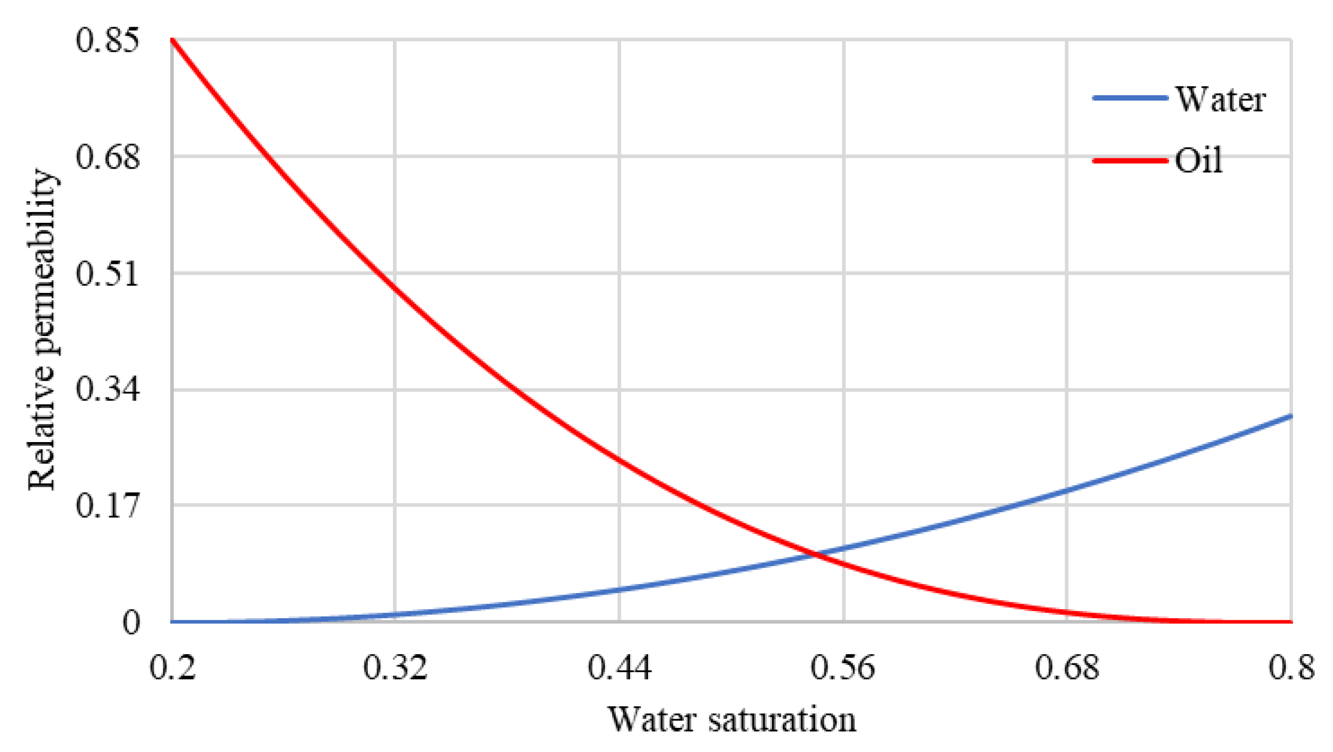
2.1. Main Governing Equations

The simulator used in this paper integrates the reservoir, fracture, and wellbore domains. The main governing equations related to this paper are summarized as follows.
Γ [ ( 2 μ + λ ) n · u n + λ n t r ( t u t ) + μ n · u t + μ t u n + σ 0 + α p I ] d Γ = 0
( V p 0 c f V t p ) p t V b · k = 1 n c + 1 V t k · j = 1 n p [ ξ j x i j k r j μ j k · ( p + p c r j ρ j g D ) + ϕ ξ j S j K · x i j ] k = 1 n c + 1 V t k q k = 0
N i t V b · j = 1 n p 1 [ ξ j x i j k r j μ j k · ( p + p c r j ρ j g D ) + ϕ ξ j S j K · x i j ] q i = 0
1 c V V t c t 1 V V t p f p f t i = 1 n c + 1 [ V t N i · ( j = 1 n p ξ j x i j k r j μ j w 2 12 p f ) ] = i = 1 n c + 1 V t N i q I n i q L e a k i V
N i t · j = 1 n p [ ξ j x i j k r j μ j w 2 12 ( w S ) · p ] = q I n i q L e a k i
V p i t + j = 1 n p · ( u p i j γ i j V p i ) = q p i
P B H P P B H P o l d K f V w e l l ( q i n i = 1 n q i ) Δ t = 0
p B H P Δ p s e c t i o n Δ p p e r f = p f
k f = d p 2 ( 1 c ) 3 c 2 [ 150 + 4.2 ( D p ρ f v f μ f c ) 5 6 ]
where λ is the Lame first parameter, μ is the Lame second parameter, n is the surface normal vector, u n is the normal displacement, u t is the tangential displacement, σ 0 is the in-situ stress, α is the Biot’s coefficient, p is the pore pressure, Γ is the surface area, N i is the moles for component i , V b is the bulk volume, n p is the number of phases, x i j is the mole fraction of component i in phase j , ξ j . k r j , μ j , p c r j , ρ j , S j , u p j are the molar density, relative permeability, viscosity, capillary pressure, mass density, saturation, and proppant velocity of phase j . k is the matrix permeability, D is the depth, ϕ is the porosity, K is the diffusion coefficient, q i stands for the source/sink term which may come from the leak-off from the fracture or a well model, V t is the total fluid volume, V p 0 is the original pore volume, c f is the formation compressibility, w is the fracture width, S is the fracture surface area, q I n i is the source term due to fluid injection/production from/into the wellbore domain, q L e a k i is the source term due to fluid leak-off into/from the reservoir domain,   V p i , q p i are the volume and volumetric injection rate of proppant i , γ i j is the phase partitioning factor of proppant i in phase j ,   ρ f is the fluid density, v f is the fluid velocity, c is the proppant concentration, and k f is the propped fracture permeability.
Equation (1) to Equation (3) are the solid deformation equation, fluid momentum conservation equation, and fluid mass conservation equation in the reservoir domain. Equation (4) to Equation (6) are the slurry momentum conservation equation, fluid mass conservation equation, and proppant volume conservation equation in the fracture domain. Equations (7) and (8) describe the slurry distribution among clusters. Equation (9) formulates the permeability of propped fractures. All the governing equations in our model are discretized in space, using the finite volume and finite area methods and in time using the backward Euler method. The coupled systems of equations are solved using the Newton-type formulations. Readers are encouraged to refer to the previous publications for more details in the governing equations, solution algorithms, model implementation, and model validation [9,22,23,24,25,26,27].

2.2. Modeling of Foam Rheology

In the previous work, the water-based fracturing fluid is modeled as a Newtonian fluid with constant viscosity and the viscosity of gas fracturing fluid is modeled using the Lohrenz-Bray-Clark correlation [28]. However, many hydraulic fracturing fluids such as gel and foam are non-Newtonian fluids, and their viscosity is a strong function of shear rate. Typically, they can be modeled as a shear thinning power low fluid. In this work, we extend the model to include the power-law fluids. We have implemented a general formulation (10) to describe the fracturing fluid viscosity as a function of the pressure gradient and width inside the fracture as well as fluid rheology parameters by [29].
μ f = ( 2 n + 1 6 n ) ( 2 k ) 1 n ( w p ) 1 1 n
where μ f is the viscosity of fracturing fluid, p is the pressure gradient within the fracture, k and n are the fluid consistency index and behavior index. Regarding the effect of proppant on the viscosity increase of the proppant laden, [29] adopt the method by [30] to describe k and n as functions of proppant concentration. However, the parameters in the functions are different for different fracturing fluids and need to be measured by experiments. In this paper, we keep our correlation (11) to be the same as [31].
μ s = μ f [ 1 + 1.25 c 1 c / c m a x ] 2
where μ s is the viscosity of the slurry and c m a x is the packing concentration of proppants.
When the simulator is used to model foam, in the fracture domain, there are two phases: a water phase and a hydrocarbon phase, and the two phases are considered to flow as one pseudo-phase. The viscosity of the two phases is calculated using the above viscosity formulation using the input values for k and n . The density of the gas phase is calculated using the EOS. The slurry density is calculated using the volume average of water, hydrocarbon, and proppant densities. Since one pseudo-phase is considered, we assume the foam is stable and there is no velocity difference between the water and gas phase. Thus, the two phases are flowing at the same velocity and proppants are considered to flow in the pseudo-phase.

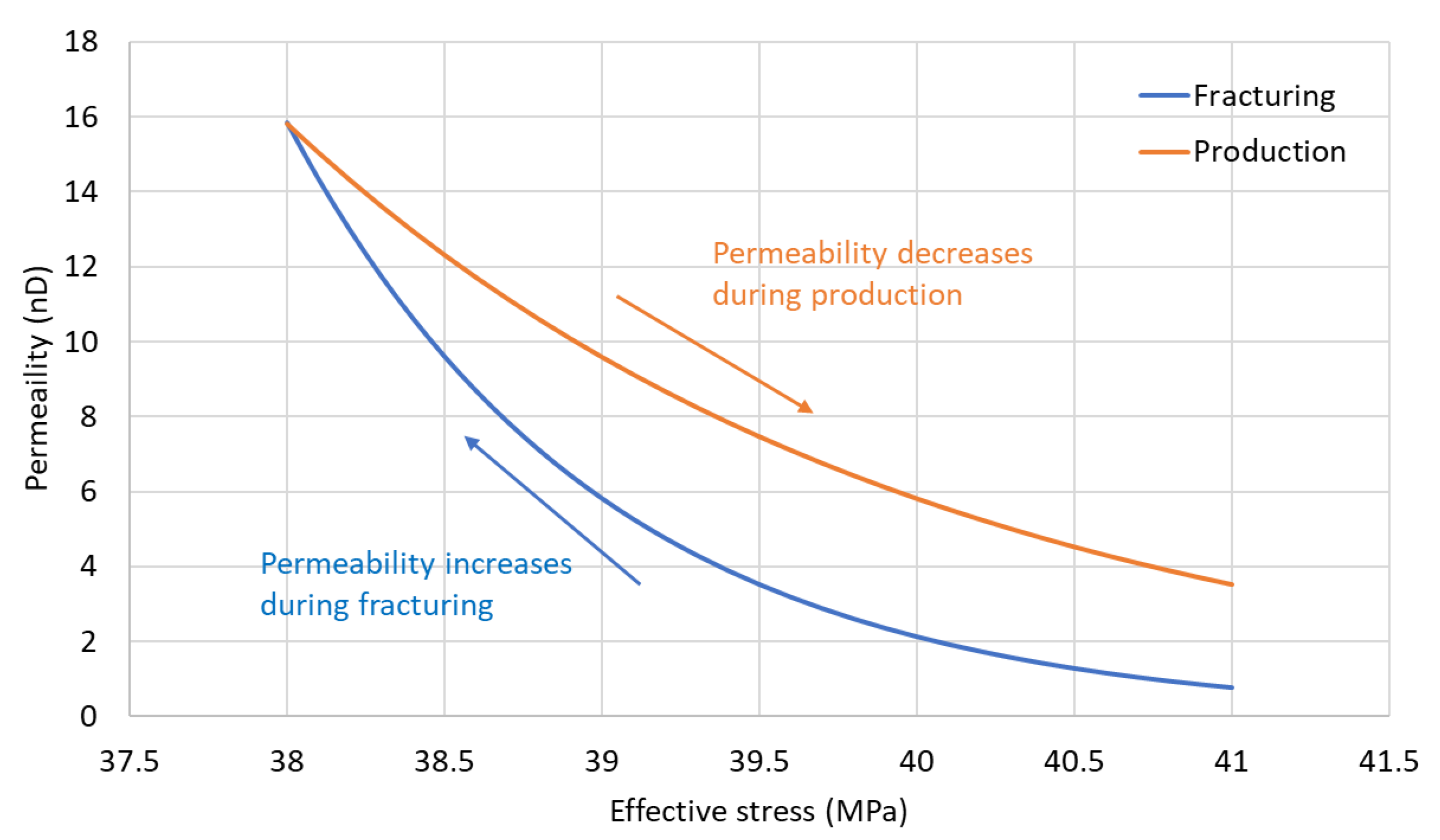
2.3. Stress Dependent Permeability
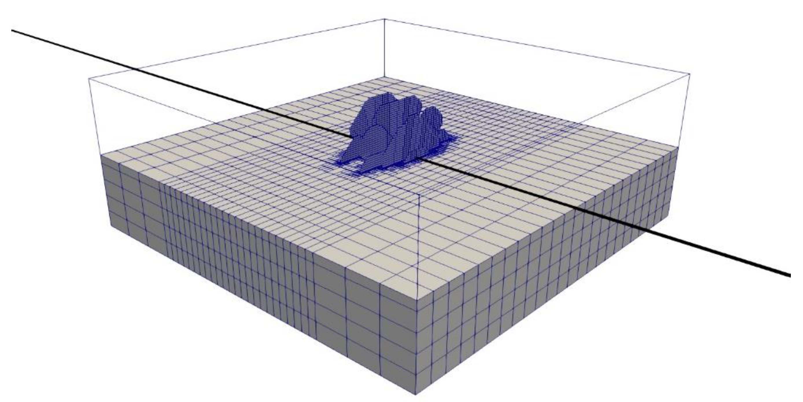
Changes in permeability and porosity because of the reservoir depletion or recharging are important in stress-sensitive reservoirs [32]. During hydraulic fracturing, in addition to the main hydraulic fracture growth, there are numerous micro-cracks created, forming an SRV region, and there is an enhanced permeability in the SRV region. During production, the hydraulic fractures and micro-cracks close, and the enhanced permeability decreases as the pressure decreases and the effective stress become more compressive. In the past, linear relationships, exponential relationships, and fractal models have been proposed to model the dynamically changing SRV permeability [33]. In the exponential relationship, the SRV permeability is usually described as an exponential function of pore pressure or effective stress. In this paper, we adopt the exponential relationship and model the SRV permeability as an exponential function of the effective stress as shown in Equation (12).
k = k 0 e γ ( σ σ 0 )
where k is the matrix permeability, k 0 is the initial matrix permeability, σ is the effective stress, σ 0 is the initial effective stress, and γ is the permeability-stress exponent that can be obtained from experiments or history matching the field data.
An illustration of stress-dependent permeability changing with effective stress during hydraulic fracturing and production is shown in Figure 5. During hydraulic fracturing, the permeability increases because of the formation of micro-fractures around the main hydraulic fractures and a decrease in the effective stress (it becomes more tensile). A larger change in the effective stress indicates a larger stress shadow and more micro-cracks, leading to a larger SRV permeability enhancement. The stress and permeability at the beginning of the production simulation are saved and used as initial stress and permeability for the production simulation. During production, pore pressure decreases, causing the effective stress to become more compressive, and the SRV permeability gradually decreases, representing the closure of the micro-cracks. Different permeability-stress exponents may be used for the hydraulic fracturing and production periods.

3. Case Setup

Per estimates made by the U.S. Geology Survey (USGS), the Wolfcamp shale contains 20 billion barrels of oil and 16 trillion cubic feet of gas. The recoverable oil in the Wolfcamp shale is also estimated to be three times larger than the Bakken-Three Forks shale [34].
Given the huge amount of associated natural gas in the Wolfcamp formation in the Permian Basin and the fast growth of shale oil development and flared gas in the State of Texas (Figure 1), we conducted this simulation study using different kinds of fracturing fluids in the Permian Basin. Layer properties and fluid properties are the two key sets of inputs for our simulator. Because of data confidentiality, very limited field data in the Permian Basin is publicly available. Ref. [35] presented fracture geometry characterization in the Permian Basin using integrated microseismic, completion, and production data. Ref. [36] studied the impact of parent well depletion on stress changes and infill well completion. In this paper, we inherit the published layer data from Patterson and Sangnimnuan to build up our geological model. We focus on the Wolfcamp shale formation (A1, A2, A3, B1, B2, B3). Porous properties (porosity and permeability), mechanical properties (Young’s modulus and Poisson’s ratio), and initial conditions (water saturation and temperature) vary between different Wolfcamp shale layers as shown in Table 2. It is worth noting that in this paper, an isothermal condition is assumed which means the temperature in Table 2 will be used directly. This is because the total injection volume is small and thermo-elasticity is only important when injecting a large amount of cold fluid into the reservoir (e.g., during the water flooding).
Our equation-of-state compositional simulation requires a PVT model for the reservoir fluids. [37] studied the effect of fluid phase behavior on well production, in which they reviewed several PVT reports in the Wolfcamp, but only black-oil properties were released in their paper. [38] presented a study on the effect of injection gas composition for huff-n-puff improved oil recovery in the Permian reservoirs in which they presented a Peng-Robinson EOS model of a Wolfcamp live oil sample. Component mole fractions ( z ), critical pressure ( P c ), critical temperature ( T c ), molar weight ( M w ), binary interaction parameters (BIP) of this oil sample are presented in their paper, but other data such as acentric factor ( α ), critical volume ( V c ), and volume shift parameters were not included. In this paper, we adopt the fluid data presented by [38] and added reasonable estimates for acentric factor and critical volume for the Wolfcamp oil sample. The component mole fraction and critical properties are listed in Table 3. The binary interaction parameters between different hydrocarbon components are listed in Table 4.
Stone-II relative permeability model is used to model the relative permeability of different mobile phases and the water and oil relative permeability as a function of the water saturation is shown in Figure 6.
Other important input parameters are listed in Table 5. In the simulation, the well landing depth is 2577 m, which is in the Wolfcamp B2 formation. We use the same completion design for different hydraulic fracturing fluids, which is 10 perforation clusters per stage and 3 perforations per cluster. The cluster spacing is set to be 15 m. The initial perforation diameter is set to be 1.27 cm and perforation erosion and perforation diameter increase are modeled using the methods proposed by [39,40].
A computation domain with a size of 960 × 960 × 360   m 3 is set up for fracture propagation and shut-in simulation as shown in Figure 7. The well is landed in the middle of the domain (true vertical depth = 2577   m ). Layer properties summarized in Table 2 are assigned to each cell according to the depth. We simulate the fracture propagation and shut-in of one stage. In the production simulation, a reservoir simulation box with a size of 150 × 400 × 280   m 3 is selected within the computation domain and cells outside the box are set as null blocks, which is a representation of the control reservoir volume of this particular stage.
In the simulation, we first simulate fracture propagation for a one-hour slurry injection schedule. Three separate cases are run using slick water, 0.7 quality NG foam 30 ppt J580, and hybrid NG (first 10 min), and 0.7 quality NG foam 30 ppt J580 (last 50 min). The viscous properties of the three fracturing fluids are shown in Figure 2 and Table 1. The slurry pumping rate is set to 0.15 m 3 / s . Proppant laden fluid is injected starting from 10 min. A 100-mesh proppant is injected from 10 min to 30 min and a 30/50-mesh proppant is injected from 30 min to 60 min. The proppant volume fraction ramps up gradually every 10 min and reaches 20% in the last 10 min (Figure 8). The composition of natural gas used in the simulation is assumed to be 70% C1, 20% C2, 5% C3, and 5% C4. After one hour of injection, the well is shut-in for 5 days. During the shut-in time, the fractures are allowed to grow further (tip extension) and close. Fracturing fluid (water and gas) continues to leak-off into the reservoir and proppant settles inside the fractures. After the shut-in period, the well is produced for 5 years with a decreasing downhole pressure from 32.8 MPa (initial pore pressure) to 10 MPa for the duration of the production time. Cumulative surface oil, gas, and water production rates are computed.

4. Results and Discussion

Simulation results during the injection, shut-in, and production periods are compared and analyzed in this section to demonstrate the differences in the performance of the different fracturing fluids.

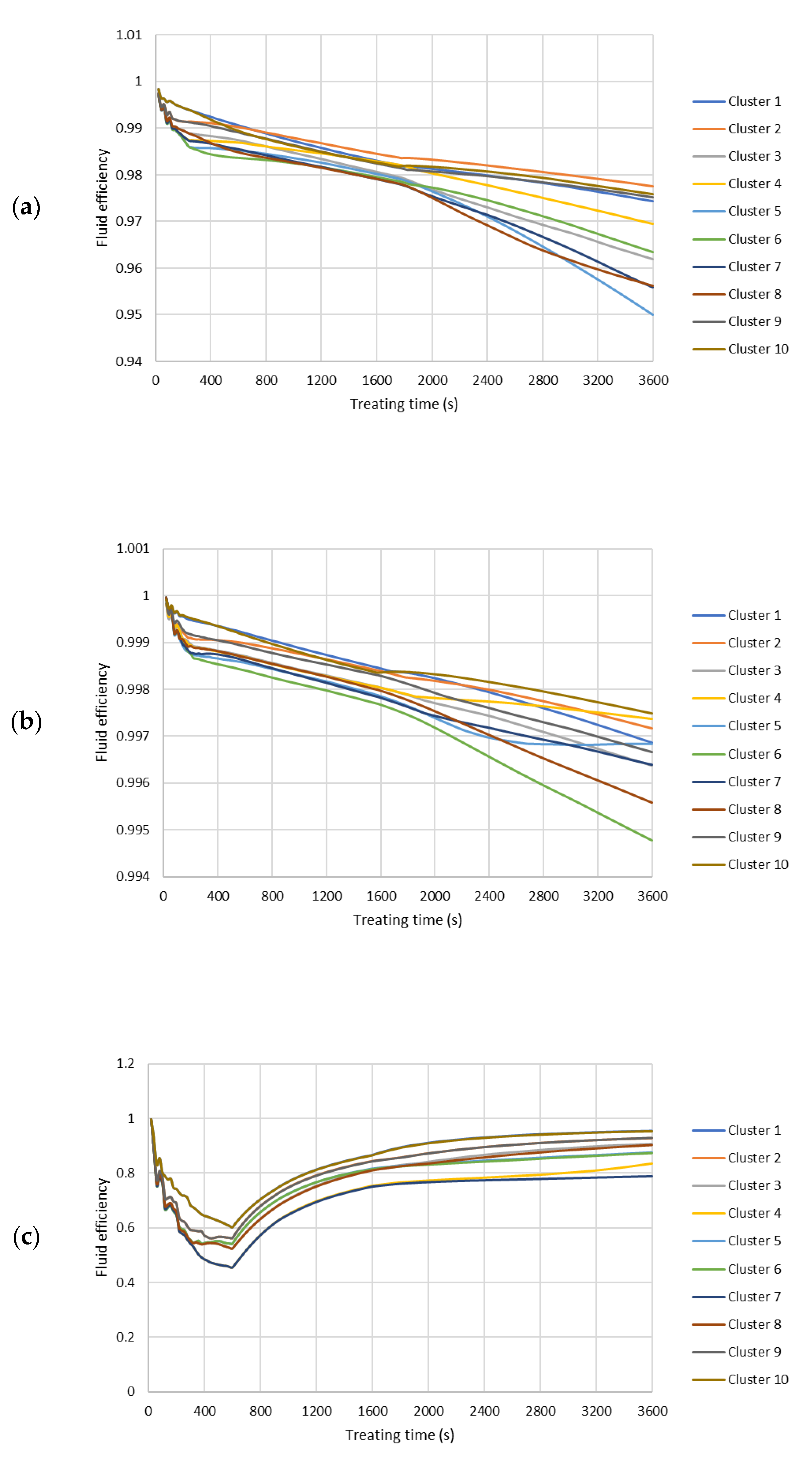
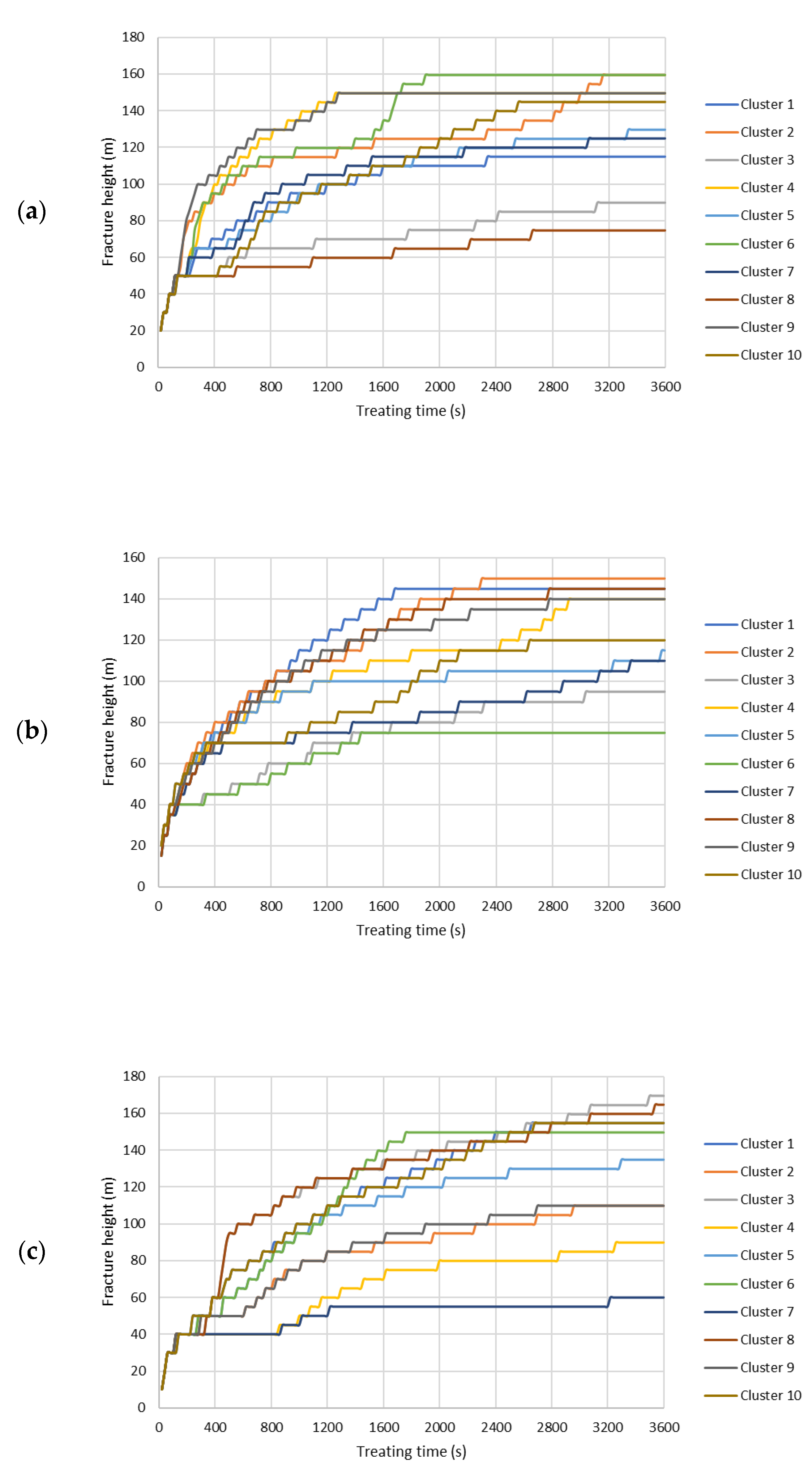
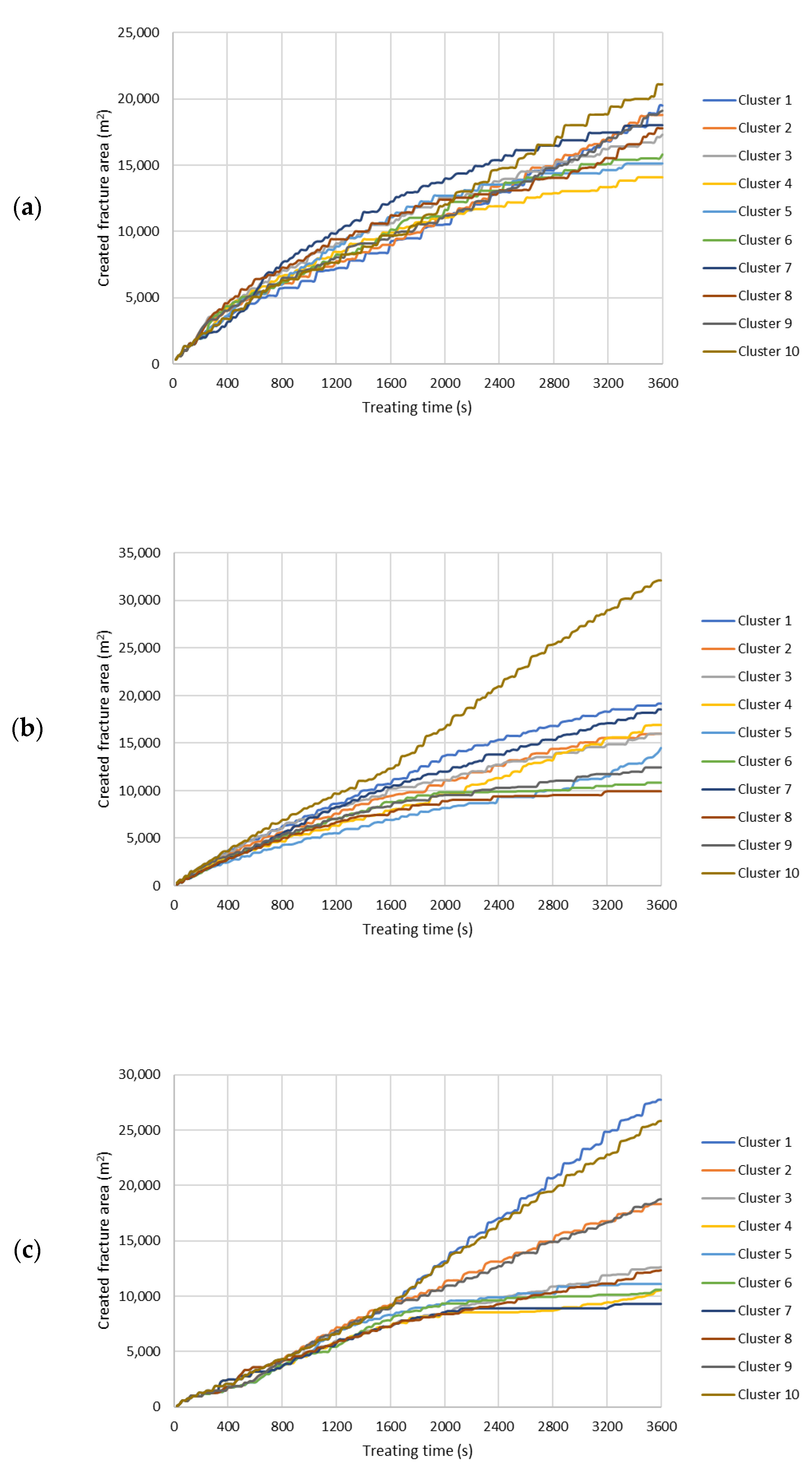
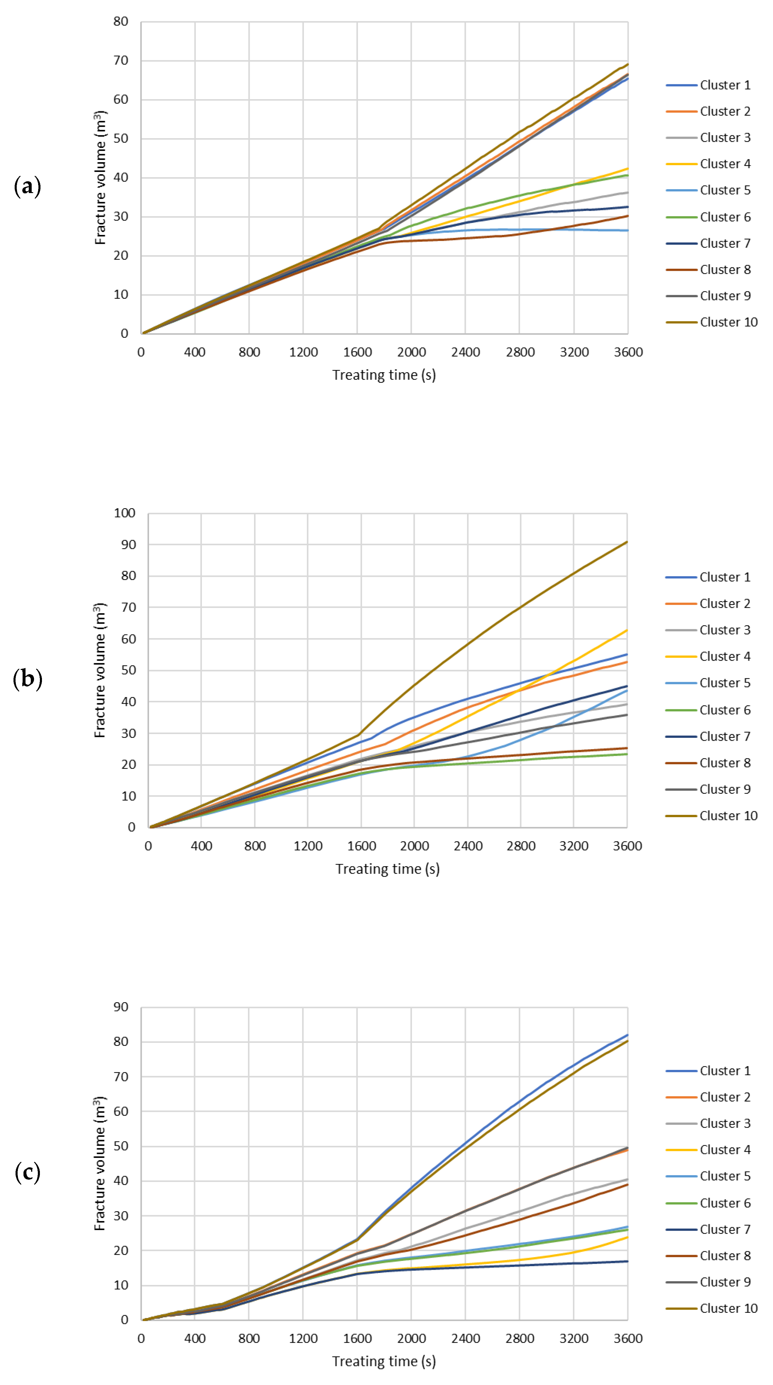
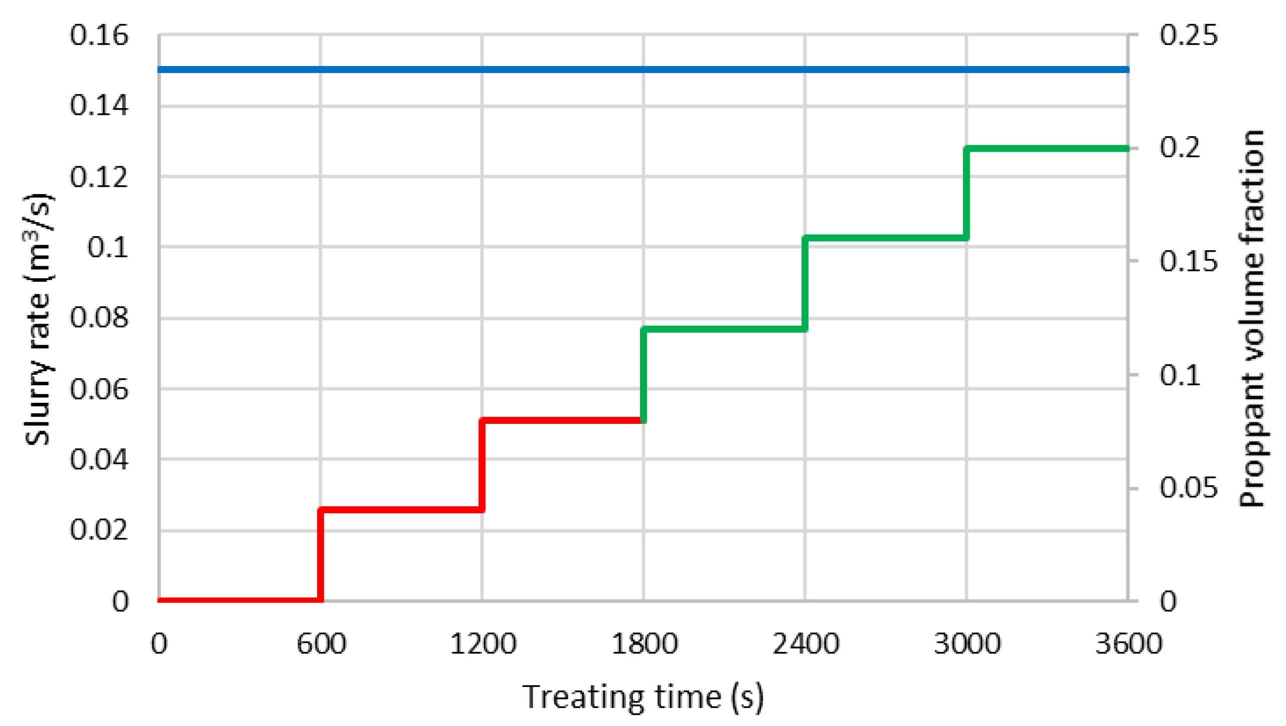
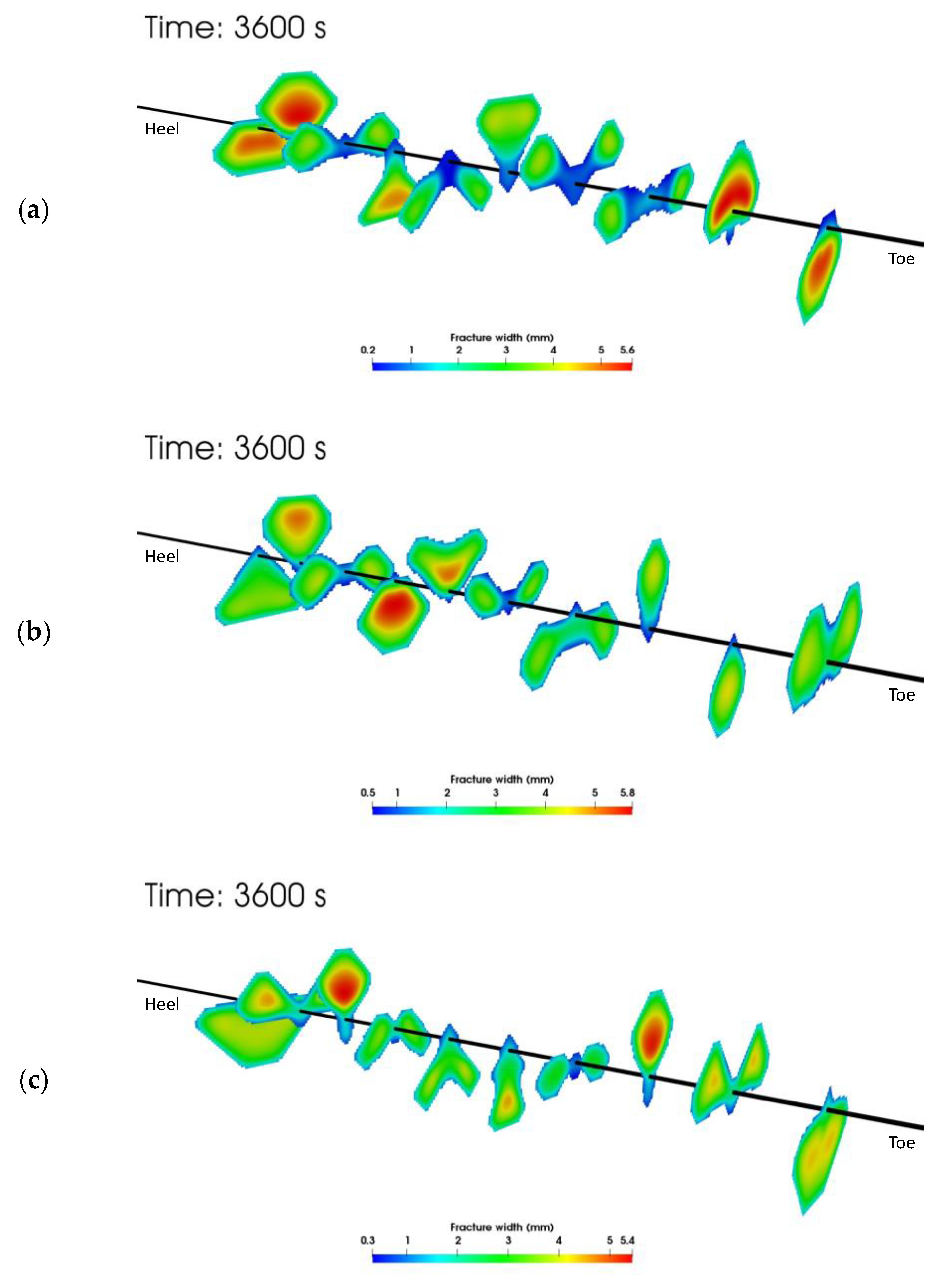
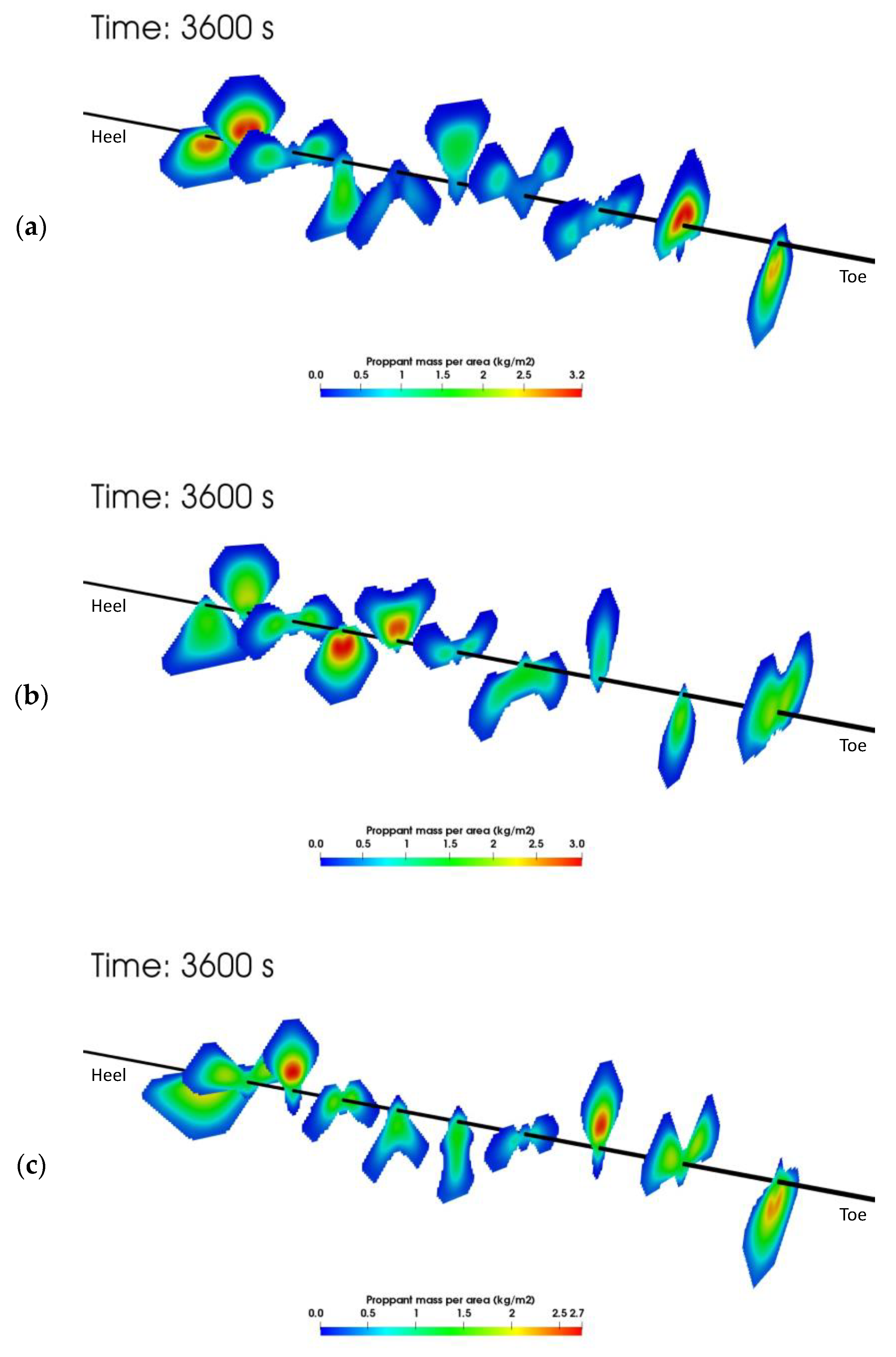
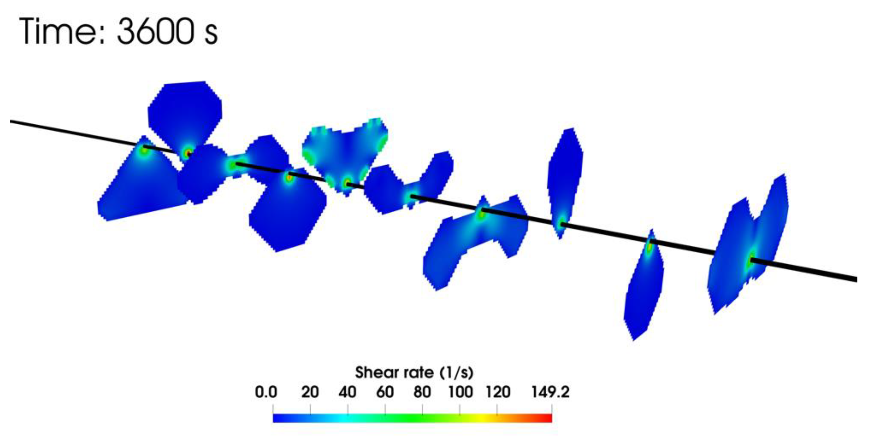
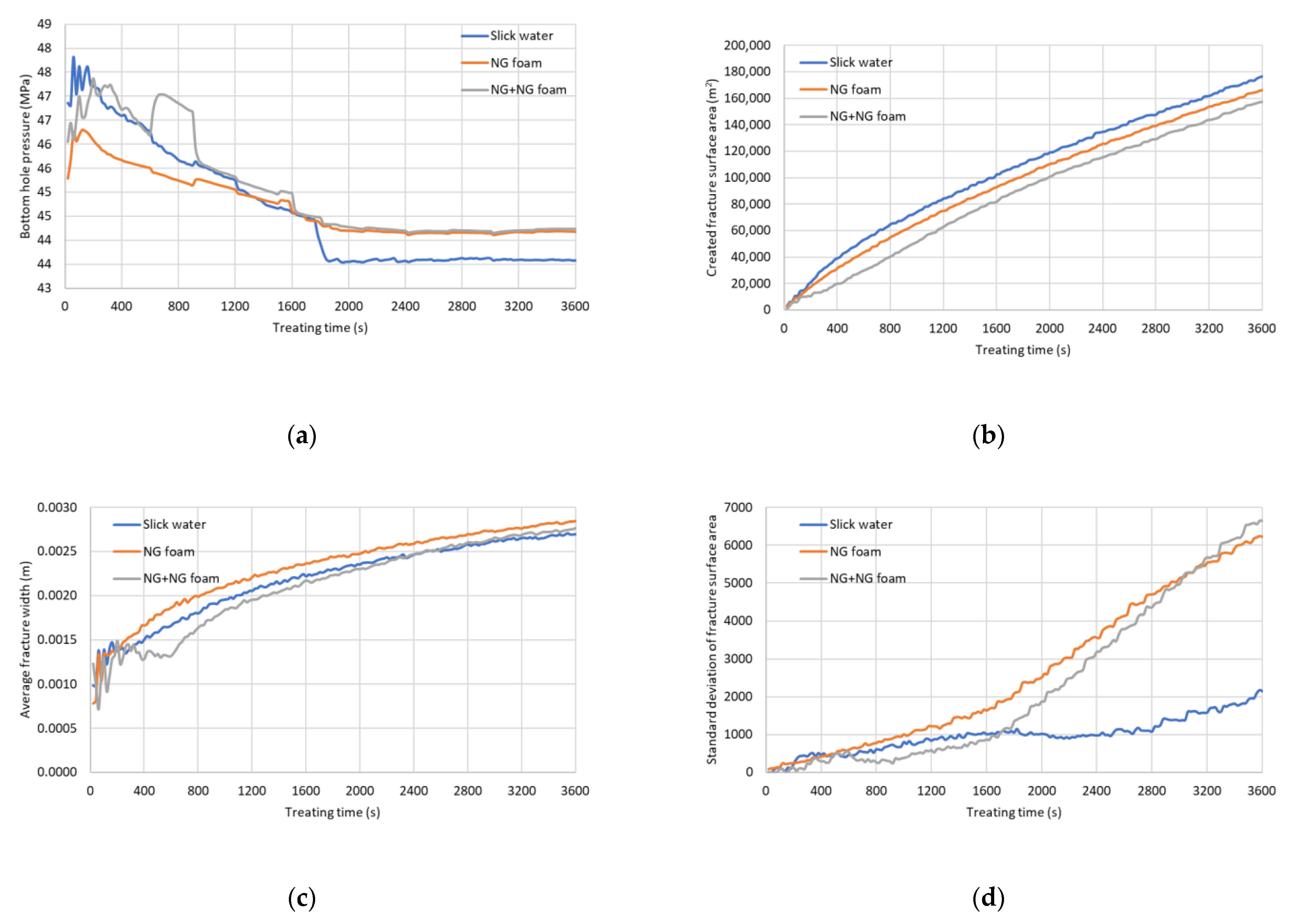
4.1. Results for the Injection Period

Figure 9 shows the fracture width distribution at the end of the one-hour slurry injection period. One trend seen in all three sets of simulation is the non-uniform growth of the hydraulic fractures. Because of the stress shadow between all the growing fractures (which has been considered implicitly in our model by solving the solid deformation equation), adjacent fractures propagate in a way to achieve the least overlapping area. It is also observed that the fracture width varies more in the slick water case than in the two NG foam cases. By comparing the two NG foam cases, one can find that the case using hybrid NG and NG foam gives a smaller fracture surface area than the case using pure NG foam, as the injection of low-viscous pure NG causes larger leakoff and less fracture propagation. Since we do not know the real stress profile in the Wolfcamp formation, a single minimum horizontal stress value (41.34 MPa ) is applied to all the layers. The fracture geometry may be different if a different stress profile is put into the simulator.
Figure 10 shows the proppant mass per unit area plots at the end of the one-hour treatment in the three cases. It is found that hydraulic fracturing using foam (Figure 10b,c) leads to better propped hydraulic fractures than slick water (Figure 10a). The created fracture surface and the propped fracture surface area are also calculated as shown in Table 6. We define the propped fracture to be the part of the fracture with an average of at least one layer of proppant. It can be clearly seen that slick water is able to create a larger fracture surface area than the foam cases but the propped surface area in the slick water case is smaller than the foam cases. The propped area in the foam cases is around 10% larger than the slick water case. Two reasons can explain this fact. The first reason is that foam typically has a higher viscosity than slick water, even under high temperature and high shear rate conditions inside the fractures. Thus, it has less leakoff and creates fractures with larger apertures, which makes it easier for proppant to flow and reduces the pinch point effects. The second reason is that foam with higher viscosity has better sand carrying capability than lower viscosity slick water, especially for complex height growth scenarios.
The shear rate for the fracture flow at the end of the injection period is shown in Figure 11. We notice that the shear rate is within the experimental measurement range reported by [7].
Fracturing Fluid Created   Fracture   Surface   Area   ( m 2 ) Propped   Fracture   Surface   Area   ( m 2 ) Ratio of Propped Area to the Created Area
Slick water176,65568,1480.3858
NG foam166,378.579,3200.4767
NG and NG foam159,01677,7240.4888
Other properties for fractures from each cluster can also be visualized for detailed analysis for the three simulation cases. In Appendix A, we include the fluid efficiency, fracture half-length, fracture height, created fracture surface area, created fracture volume, cumulative proppant mass, and propped fracture surface area for each cluster during hydraulic fracturing.
Figure 12 contains four sub-plots showing the individual properties changing with treating time for the three cases. Figure 12a shows the bottom hole pressure versus treating time. Slick water shows the highest breakdown pressure whereas cases using foam have a lower breakdown pressure. This is mainly because of the high compressibility of the NG foam (gas phase in foam has high compressibility). For the hybrid case, one can observe a big bump after 10 min of injection when NG foam is injected into the wellbore following the previous injected NG and the friction suddenly increases. Figure 12b shows the created fracture surface area versus time. As expected, the slick water case gives the largest created fracture surface area while the hybrid case gives the lowest fracture surface area, but the difference is not significant (around 6 percent). This is because slick water has a lower viscosity and lower compressibility and tends to create longer fractures. Foam has a higher viscosity and higher compressibility and tends to create shorter fractures. Natural gas has the lowest viscosity and highest compressibility and tends to create the shortest fractures. Figure 12c shows the average fracture width versus treating time. As expected, foam gives the largest average fracture width and gas gives the smallest fracture width. Figure 12d plots the calculated standard deviation of fracture surface area for each cluster. A larger standard deviation means more non-uniform fracture growth and a smaller standard deviation implies that the fractures from each cluster are growing more uniformly. It is found that foam cases yield more non-uniform fracture growth compared to the slick-water cases, which may cause potential parent-child well interaction problems in a newly developed field [36,41].
From the simulation results, we can calculate the total amount of fracturing fluid that is used in the treatment. The total mass of water in this stage for the slick water case is 486 tons. The total mass of the natural gas and water in this stage for the NG foam case is 112.68 and 145 tons, respectively (using the pumping schedule shown in Figure 8). Supposing this well has 30 stages, then in the slick water case, 14,580 tons of water is used. In the NG foam case, the total mass of natural gas and water used in the fracturing job are 3380.4 and 4350 tons. By comparison, 10,230 tons of water can be saved using the 0.7 quality NG foam as the fracturing fluid instead of water.

4.2. Results for the Shut-In Period

The well is then shut-in for 5 days after the one-hour slurry injection. At an early time, immediately after shut-in, water hammer effects are visible during which there is complex slurry redistribution among clusters and wellbore. As Figure 13 illustrates, during the shut-in time, some fractures obtain more fluids and fracture tip extension happens in some of the clusters and the fractures from these clusters grow further. Slurry comes out of the other fractures and flows back into the wellbore because of fracture closure caused by the complex stress shadow effects from the adjacent clusters. Figure 13 also indicates that the water hammer effect mainly happens at the first several hours of injection and gradually dies away. Moreover, Figure 13 demonstrates the strong capability of our simulator in lifecycle modeling.
Fracture closure and fluid leakoff happen throughout the shut-in time. Figure 14 shows the pore pressure changes on the horizontal plane that crosses the wellbore after the shut-in time for the three cases. Comparing Figure 14a,b, one can observe that the slick water case has more fluid (water) leaking into the reservoir than fluid (NG and water) leaking into the reservoir in the NG foam case because of the high viscosity of foam. However, more water leak-off into the reservoir is potentially harmful to the reservoir and may cause severe damages including clay swelling, relative permeability reduction, and water blocking which can be extremely harmful to gas wells. The leaked water in the reservoir is also hard to flow back because of micro-crack closure and capillary pressure effects. On the contrary, the use of foam can minimize the water invasion into the reservoir and more natural gas, which is miscible with the reservoir hydrocarbon fluid can flow into the reservoir and mitigate the impact of water leak-off. A large pore pressure increase can be seen in the near-wellbore region in Figure 14c for the hybrid case, which is the result of pure NG injection. NG flow into the reservoir can potentially benefit oil production by lowering the hydrocarbon viscosity, increasing oil relative permeability, and building up pore pressure.
We plot the cumulative fluid efficiency as a function of time during the hydraulic fracturing time period (first 1 h) and the shut-in period (from 1 h to 5 days) for the three fracturing fluid designs (Figure 15). We notice that the fluid efficiency of the slick water and NG foam is very high during the hydraulic fracturing period, which indicates that the leakoff is very low for both cases. For the hybrid NG and NG foam case, during the NG injection (first 10 min), the fluid efficiency is very low, which is due to the fact that NG viscosity is very low, leading to larger leakoff. During the NG foam injection (last 50 min), the fluid efficiency increases due to the increasing fluid viscosity and decreasing leakoff by the NG foam. During the shut-in period, the fluid efficiency decreases in all three cases because no more slurry is injected into the wellbore and more fluid leaks off into the reservoir during the 5-day shut-in. It can also be observed that 90% of slick water leaks into the reservoir whereas only 50% of the NG foam leaks into the reservoir because of the difference in the fluid viscosity and reservoir permeability enhancement. This indicates the advantage of easier flowback for the NG foam fracturing fluids.

4.3. Results for the Production Period

After the shut-in period, the well is produced for 5 years. The downhole pressure is decreased from 32.8   MPa to 10   MPa in the first 100 days and is fixed at 10   MPa in the following production period. Figure 16 shows the pore pressure distribution within the horizontal plane across the wellbore at the end of the production period. Only the region within the stage of focus is being depleted because of the fact that the grid blocks outside the stage of focus are set to be null blocks. One can observe that the pore pressure in the matrix is larger in the slick water case than in the two foam cases. This is because of the low residual fracture width and poor sand placement near the wellbore regions after the shut-in as indicated by Figure 9 and Figure 10. Poor proppant placement in some clusters near the wellbore leads to low propped fracture conductivity. The unpropped fracture part will close and form pinch points after the shut-in, which prevents the reservoir fluid from flowing through those fractures into the wellbore. The fractures from these clusters may contribute less to the production of the full well. This results in low cluster efficiency and lower well productivity. Thus, the fractured reservoir volumes with unpropped fractures will produce less and the pore pressure will remain high. The fractured reservoir volumes with well-propped fractures will produce more and the pore pressure will be low. Comparing the three depleted reservoir pressure profiles in Figure 16, we found that the reservoir is better depleted in the NG foam case and the hybrid NG and NG foam case. This is because of the better sand placement in the two foam cases as shown in Figure 10 and Table 6.
The cumulative oil and gas production versus production time at surface conditions is listed in Table 5 and plotted in Figure 17. We observe that the cases using NG foam or hybrid NG and NG foam give much higher production than the case using slick water. An increase of 95% and 65% in oil production is observed from the simulation. A similar trend is also observed in cumulative gas production. As discussed in the previous parts of this paper, several reasons are contributing to the production of foam fractured wells surpassing the slick water fractured well. (1). More microcracks are created (reflected by a larger change in the effective stress) using NG foam and NG, and thus higher SRV permeability enhancement. (2). Created fractures are better propped using NG foam, and thus higher cluster efficiency. (3). NG enters the reservoir and reduces the amount of water entering the reservoir, benefiting the oil production by relative permeability improvement, viscosity reduction, and energizing the reservoir.
Some final important caveats to the application of our results: First, since this is a simulation study and many assumptions have been made in the simulation, the field implementation of this strategy may yield less favorable results when using the NG foam. More precise data input, model calibration with existing field data, and field pilot tests are still essential to obtain more predictive results of NG foam fracturing. Second, safety concerns associated with the use of NG and NG foam may prevent the use of such fluids in many instances in the field. These concerns can also potentially increase the cost of pumping such fluids (even when the gas is available for free). These safety concerns are offset by the benefits of a substantial reduction in flaring of produced natural gas.

5. Conclusions

An equation of state compositional hydraulic fracturing and reservoir model has been extended to include the modeling capability of non-Newtonian fracturing fluid for hydraulic fracturing in this paper. We built a precise layer model and fluid model using published data from the Wolfcamp formations in the Permian Basin and performed lifecycle analysis to the reservoir. We simulated hydraulic fracture propagation using slick water, NG foam, and hybrid NG and NG foam, shut-in and fracture closure, and long-term production. Results from different periods of the well lifecycle are visualized and analyzed. The key findings are summarized below:
  • The use of NG foam reduces both gas flaring and water usage in well completions potentially saving both capital and reducing the environmental impact. The simulation results presented here can be used to conduct an economic analysis that includes the drilling cost, completion cost, additional cost for gas storage and foam generation, oil/gas/water daily production, oil price to evaluate the cash flow performance of different fracturing fluids and completion designs.
  • The use of NG foam gives lower breakdown pressure, smaller created fracture surface area, and larger average fracture width during the hydraulic fracturing than slick water.
  • NG foam causes higher effective stress (more compressive) and a larger stress shadow effect than slick water during hydraulic fracturing. More microcracks and higher SRV permeability are expected using NG foam.
  • NG foam has a significantly better sand transport capacity and can thus achieve better proppant placement inside the fractures.
  • Higher cluster efficiency and higher oil and gas productivity are observed using NG foam than slick water.
  • NG foam leads to more non-uniform fracture growth which may leave unstimulated regions in a newly developed reservoir.
  • Precise data input, model calibration, and field pilot tests are essential to obtain more accurately predictable results for NG foam fracturing.

Author Contributions

Conceptualization, S.Z. and M.M.S.; methodology, S.Z. and M.M.S.; software, S.Z.; validation, S.Z.; formal analysis, S.Z.; investigation, S.Z.; resources, M.M.S.; data curation, S.Z.; writing—original draft preparation, S.Z. and M.M.S.; writing—review and editing, S.Z. and M.M.S.; visualization, S.Z.; supervision, M.M.S.; project administration, M.M.S.; funding acquisition, M.M.S. All authors have read and agreed to the published version of the manuscript.

Funding

This research received no external funding.

Acknowledgments

We would like to express our gratitude to the Hydraulic Fracturing and Sand Control Industrial Affiliates Program at the Center for Subsurface Energy and the Environment at the University of Texas at Austin for supporting this research.

Conflicts of Interest

The authors declare no conflict of interest.

Appendix A

In this Appendix, the properties of each cluster during the fracturing simulation are plotted for the three simulation cases, respectively. Figure A1 shows the fluid efficiency of each cluster. Figure A2 shows the fracture half-length of each cluster. Figure A3 shows the fracture height of each cluster. Figure A4 shows the created fracture surface area of each cluster. Figure A5 shows the fracture volume of each cluster. Figure A6 shows the cumulative proppant mass into each cluster. Figure A7 shows the propped fracture surface area of each cluster.
Figure A1. Fluid efficiency of each cluster during the hydraulic fracturing treatment. (a) Slick water case. (b) NG foam case. (c) Hybrid NG/NG foam case.
Energies 14 07645 g0a1
Figure A2. Fracture half-length of each cluster during the hydraulic fracturing treatment. (a) Slick water case. (b) NG foam case. (c) Hybrid NG/NG foam case.
Energies 14 07645 g0a2
Figure A3. Fracture height of each cluster during the hydraulic fracturing treatment. (a) Slick water case. (b) NG foam case. (c) Hybrid NG/NG foam case.
Energies 14 07645 g0a3
Figure A4. Created fracture surface area of each cluster during the hydraulic fracturing treatment. (a) Slick water case. (b) NG foam case. (c) Hybrid NG/NG foam case.
Energies 14 07645 g0a4
Figure A5. Fracture volume of each cluster during the hydraulic fracturing treatment. (a) Slick water case. (b) NG foam case. (c) Hybrid NG/NG foam case.
Energies 14 07645 g0a5
Figure A6. Proppant mass into each cluster during the hydraulic fracturing treatment. (a) Slick water case. (b) NG foam case. (c) Hybrid NG/NG foam case.
Energies 14 07645 g0a6
Figure A7. Propped fracture surface area of each cluster during the hydraulic fracturing treatment. (a) Slick water case. (b) NG foam case. (c) Hybrid NG/NG foam case.
Energies 14 07645 g0a7

References

  1. Ozowe, W.O.; Zheng, S.; Sharma, M.M. Selection of Hydrocarbon Gas for Huff-n-Puff IOR in Shale Oil Reservoirs. J. Pet. Sci. Eng. 2020, 195, 107683. [Google Scholar] [CrossRef]
  2. Pankaj, P.; Phatak, A.; Verma, S. Evaluating Natural Gas-Based Foamed Fracturing Fluid Application in Unconventional Reservoirs. In Proceedings of the SPE Asia Pacific Oil and Gas Conference and Exhibition, Brisbane, Australia, 23–25 October 2018. [Google Scholar] [CrossRef]
  3. U.S. Department of Energy. Natural Gas Gross Withdrawals and Production. 2021. Available online: https://www.eia.gov/dnav/ng/ng_prod_sum_dc_NUS_mmcf_a.htm (accessed on 11 October 2021).
  4. Ribeiro, L.H.N. Development of a Three-Dimensional Compositional Hydraulic Fracturing Simulator for Energized Fluids. Ph.D. Thesis, The University of Texas at Austin, Austin, TX, USA, 2013. Available online: http://hdl.handle.net/2152/22805 (accessed on 11 October 2021).
  5. Khade, S.D.; Shah, S.N. New Rheological Correlations for Guar Foam Fluids. SPE Prod. Facil. 2004, 19, 77–85. [Google Scholar] [CrossRef]
  6. Ribeiro, L.H.; Sharma, M.M. Multiphase Fluid-loss Properties and Return Permeability of Energized Fracturing Fluids. SPE Prod. Oper. 2012, 27, 265–277. [Google Scholar] [CrossRef]
  7. Beck, G.; Verma, S. Development and Field Testing Novel Natural Gas (NG) Surface Process Equipment for Replacement of Water as Primary Hydraulic Fracturing Fluid. In Proceedings of the Carbon Storage and Oil and Natural Gas Technologies Review Meeting, Pittsburgh, PA, USA, 13–16 August 2016; pp. 16–18. [Google Scholar]
  8. Beck, G.; Nolen, C.; Hoopes, K.; Krouse, C.; Poerner, M.; Phatak, A.; Verma, S. Laboratory Evaluation of a Natural Gas-Based Foamed Fracturing Fluid. In Proceedings of the SPE Annual Technical Conference and Exhibition, San Antonio, TX, USA, 9–11 October 2017. [Google Scholar] [CrossRef]
  9. Zheng, S.; Sharma, M.M. The Effects of Geomechanics, Diffusion and Phase Behavior for Huff-n-Puff IOR in Shale Oil Reservoirs. In Proceedings of the SPE Annual Technical Conference and Exhibition, Denver, CO, USA, 5–7 October 2020. [Google Scholar] [CrossRef]
  10. Lecampion, B.; Bunger, A.; Zhang, X. Numerical methods for hydraulic fracture propagation: A review of recent trends. J. Nat. Gas Sci. Eng. 2018, 49, 66–83. [Google Scholar] [CrossRef] [Green Version]
  11. Agrawal, S.; Zheng, S.; Foster, J.T.; Sharma, M.M. Coupling of meshfree peridynamics with the Finite Volume Method for poroelastic problems. J. Pet. Sci. Eng. 2020, 192, 107252. [Google Scholar] [CrossRef]
  12. Hirose, S.; Sharma, M.M. Numerical Modelling of Fractures in Multilayered Rock Formations Using a Displacement Discontinuity Method. In Proceedings of the 52nd US Rock Mechanics/Geomechanics Symposium, Seattle, WA, USA, 17–20 July 2018. [Google Scholar]
  13. Li, J.; Li, Y.; Wu, K. An Efficient Higher Order Displacement Discontinuity Method with Joint Element for Hydraulic Fracture Modeling. In Proceedings of the 55th US Rock Mechanics/Geomechanics Symposium, Houston, TX, USA, 18–25 June 2021. [Google Scholar]
  14. Ouchi, H.; Katiyar, A.; Foster, J.T.; Sharma, M.M. A Peridynamics Model for the Propagation of Hydraulic Fractures in Naturally Fractured Reservoirs. SPE J. 2017, 22, 1082–1102. [Google Scholar] [CrossRef]
  15. Settgast, R.R.; Fu, P.; Walsh, S.D.; White, J.A.; Annavarapu, C.; Ryerson, F.J. A Fully Coupled Method for Massively Parallel Simulation of Hydraulically Driven Fractures in 3-dimensions. Int. J. Numer. Anal. Methods Geomech. 2017, 41, 627–653. [Google Scholar] [CrossRef]
  16. Taleghani, A.D.; Gonzalez, M.; Shojaei, A. Overview of numerical models for interactions between hydraulic fractures and natural fractures: Challenges and limitations. Comput. Geotech. 2016, 71, 361–368. [Google Scholar] [CrossRef]
  17. Weng, X. Modeling of complex hydraulic fractures in naturally fractured formation. J. Unconv. Oil Gas Resour. 2015, 9, 114–135. [Google Scholar] [CrossRef]
  18. Wu, K.; Olson, J.E. Simultaneous Multifracture Treatments: Fully Coupled Fluid Flow and Fracture Mechanics for Horizontal Wells. SPE J. 2015, 20, 337–346. [Google Scholar] [CrossRef]
  19. Zhang, F.; Damjanac, B.; Maxwell, S. Investigating hydraulic fracturing complexity in naturally fractured rock masses using fully coupled multiscale numerical modeling. Rock Mech. Rock Eng. 2019, 52, 5137–5160. [Google Scholar] [CrossRef]
  20. Friehauf, K.E. Simulation and Design of Energized Hydraulic Fractures. Ph.D. Thesis, The University of Texas at Austin, Austin, TX, USA, 2009. Available online: http://hdl.handle.net/2152/6644 (accessed on 11 October 2021).
  21. Gu, M. Shale Fracturing Enhancement by Using Polymer-Free Foams and Ultra-Light Weight Proppants. Ph.D. Thesis, The University of Texas at Austin, Austin, TX, USA, 2013. Available online: http://hdl.handle.net/2152/28733 (accessed on 11 October 2021).
  22. Manchanda, R.; Zheng, S.; Hirose, S.; Sharma, M.M. Integrating Reservoir Geomechanics with Multiple Fracture Propagation and Proppant Placement. SPE J. 2020, 25, 662–691. [Google Scholar] [CrossRef]
  23. Zheng, S.; Manchanda, R.; Sharma, M.M. Development of a Fully Implicit 3-D Geomechanical Fracture Simulator. J. Pet. Sci. Eng. 2019, 179, 758–775. [Google Scholar] [CrossRef]
  24. Zheng, S.; Manchanda, R.; Sharma, M.M. Modeling Fracture Closure with Proppant Settling and Embedment During Shut-in and Production. SPE Drill. Completion 2020, 35, 668–683. [Google Scholar] [CrossRef]
  25. Zheng, S.; Hwang, J.; Manchanda, R.; Sharma, M.M. An Integrated Model for Multi-Phase Flow, Geomechanics and Fracture Propagation. J. Pet. Sci. Eng. 2020, in press. [Google Scholar]
  26. Zheng, S.; Manchanda, R.; Gala, D.P.; Sharma, M.M. Pre-loading Depleted Parent Wells to Avoid Frac-Hits: Some Important Design Considerations. SPE Drill. Completion 2020, 36, 170–187. [Google Scholar] [CrossRef]
  27. Zheng, S.; Sharma, M.M. An Integrated Equation-of-State Compositional Hydraulic Fracturing and Reservoir Simulator. In Proceedings of the SPE Annual Technical Conference and Exhibition, Denver, CO, USA, 5–7 October 2020. [Google Scholar] [CrossRef]
  28. Lohrenz, J.; Bray, B.G.; Clark, C.R. Calculating Viscosities of Reservoir Fluids from Their Compositions. J. Pet. Technol. 1964, 16, 1–171. [Google Scholar] [CrossRef]
  29. Yew, C.H.; Weng, X. Mechanics of Hydraulic Fracturing; Gulf Professional Publishing: Houston, TX, USA, 2014. [Google Scholar]
  30. Shah, S.N. Rheological Characterization of Hydraulic Fracturing Slurries. SPE Prod. Facil. 1993, 8, 123–130. [Google Scholar] [CrossRef]
  31. Keck, R.G.; Nehmer, W.L.; Strumolo, G.S. A New Method for Predicting Friction Pressures and Rheology of Proppant-laden Fracturing Fluids. SPE Prod. Eng. 1992, 7, 21–28. [Google Scholar] [CrossRef]
  32. Gao, C.; Gray, K.E. The development of a coupled geomechanics and reservoir simulator using a staggered grid finite difference approach. In Proceedings of the SPE Annual Technical Conference and Exhibition, San Antonio, TX, USA, 9–11 October 2017. [Google Scholar] [CrossRef]
  33. Wang, W.; Fan, D.; Sheng, G.; Chen, Z.; Su, Y. A Review of Analytical and Semi-analytical Fluid Flow Models for Ultra-tight Hydrocarbon Reservoirs. Fuel 2019, 256, 115737. [Google Scholar] [CrossRef]
  34. Gaswirth, S.B.; Marra, K.R.; Lillis, P.G.; Mercier, T.J.; Leathers-Miller, H.M.; Schenk, C.J.; Klett, T.R.; Le, P.A.; Tennyson, M.E.; Hawkins, S.J.; et al. Assessment of Undiscovered Continuous Oil Resources in the Wolfcamp Shale of the Midland Basin, Permian Basin Province, Texas; No. 2016-3092; US Geological Survey: Reston, VA, USA, 2016. [CrossRef] [Green Version]
  35. Patterson, R.; Yu, W.; Wu, K. Integration of Microseismic Data, Completion Data, and Production Data to Characterize Fracture Geometry in the Permian Basin. J. Nat. Gas Sci. Eng. 2018, 56, 62–71. [Google Scholar] [CrossRef]
  36. Sangnimnuan, A.; Li, J.; Wu, K.; Holditch, S.A. Impact of Parent Well Depletion on Stress Changes and Infill Well Completion in Multiple Layers in Permian Basin. In Proceedings of the Unconventional Resources Technology Conference, Denver, CO, USA, 22–24 July 2019. [Google Scholar] [CrossRef]
  37. Forrest, J.; Zhu, T.; Xiong, H.; Pradhan, Y. The Effect of Initial Conditions and Fluid PVT Properties on Unconventional Oil and Gas Recoveries in the Wolfcamp Formation in the Midland Basin. In Proceedings of the Unconventional Resources Technology Conference, Houston, TX, USA, 23–25 July 2018. [Google Scholar] [CrossRef]
  38. Li, L.; Sheng, J.J.; Xu, J. Gas Selection for Huff-n-Puff EOR in Shale Oil Reservoirs based upon Experimental and Numerical Study. In Proceedings of the SPE Unconventional Resources Conference, Calgary, AB, Canada, 15–16 February 2017. [Google Scholar] [CrossRef]
  39. Cramer, D.; Friehauf, K.; Roberts, G.; Whittaker, J. Integrating DAS, Treatment Pressure Analysis and Video-based Perforation Imaging to Evaluate Limited Entry Treatment Effectiveness. In Proceedings of the SPE Hydraulic Fracturing Technology Conference and Exhibition, The Woodlands, TX, USA, 23–25 January 2018. [Google Scholar] [CrossRef]
  40. Romero, J.; Mack, M.G.; Elbel, J.L. Theoretical Model and Numerical Investigation of Near-Wellbore Effects in Hydraulic Fracturing. In Proceedings of the SPE Annual Technical Conference and Exhibition, Dallas, TX, USA, 22–25 October 1995. [Google Scholar] [CrossRef]
  41. Gao, C.; Gray, K.E. A workflow for infill well design: Wellbore stability analysis through a coupled geomechanics and reservoir simulator. J. Pet. Sci. Eng. 2019, 176, 279–290. [Google Scholar] [CrossRef]
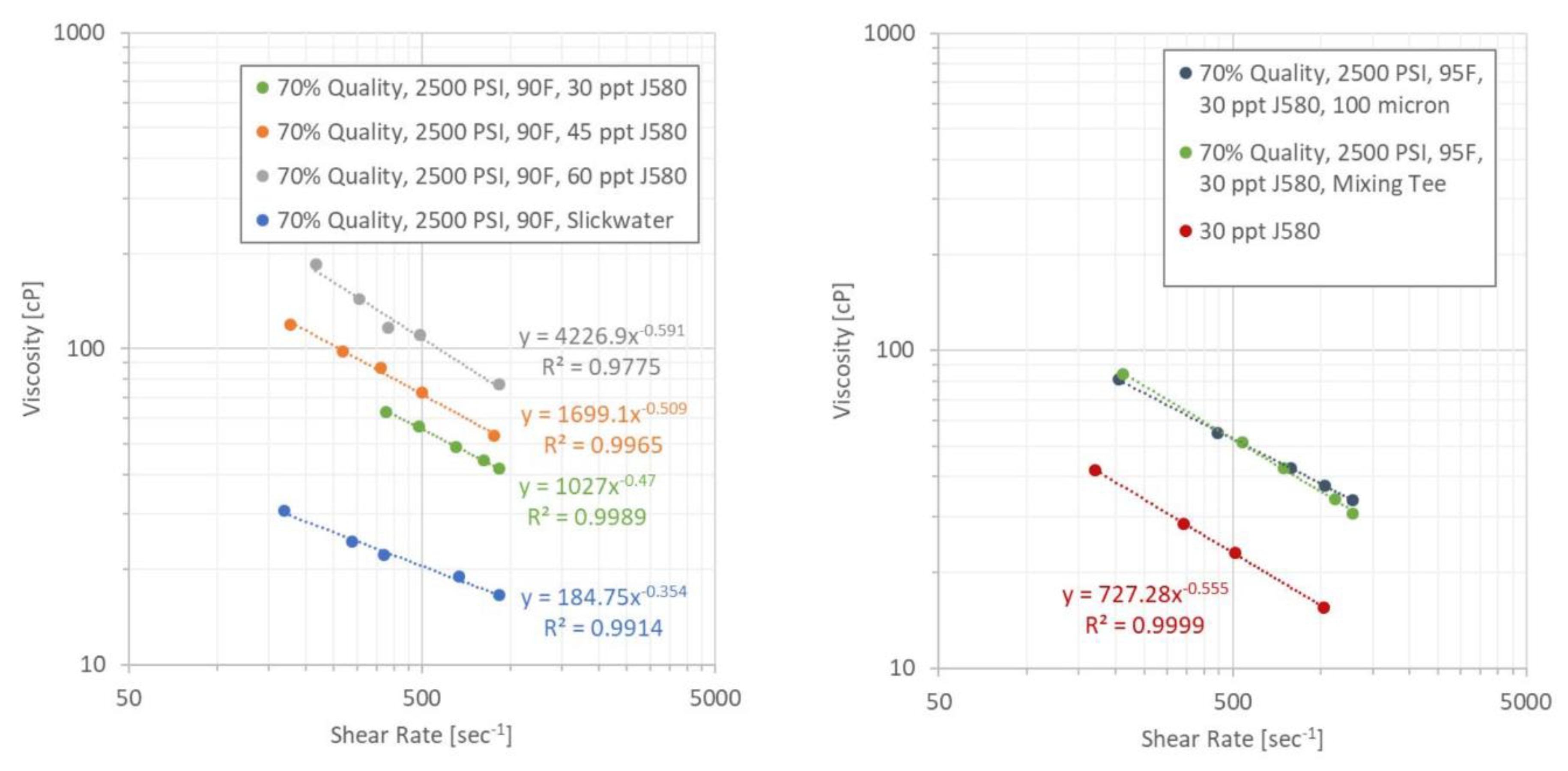
Figure 2. Viscosity versus shear rate for different NG foam and base fluids (from [2]).
Energies 14 07645 g002
Figure 3. Solution domain and coupled physics in the simulator.
Energies 14 07645 g003
Figure 4. Simulator solution algorithm (Implicit pressure, explicit concentration).
Energies 14 07645 g004
Figure 5. Illustration of stress dependent permeability changing during hydraulic fracturing and production.
Energies 14 07645 g005
Figure 6. Stone-II relative permeability model.
Energies 14 07645 g006
Figure 7. Computation domain. The black solid line represents the horizontal wellbore. The reservoir mesh for the lower-half of the domain and the fracture mesh for the upper-half of the domain are shown in the figure.
Energies 14 07645 g007
Figure 8. Treatment schedule of the hydraulic fracturing job.
Energies 14 07645 g008
Figure 9. Fracture width distribution at the end of the one-hour injection. The axis scales along the wellbore direction have been exaggerated 6 times. (a) Case using slick water, (b) Case using NG foam, (c) Case using hybrid NG and NG foam.
Energies 14 07645 g009
Figure 10. Proppant mass per unit fracture area distribution at the end of the one-hour injection. The axis scales along the wellbore direction have been exaggerated 6 times. (a) Case using slick water, (b) Case using NG foam, (c) Case using hybrid NG and NG foam.
Energies 14 07645 g010
Figure 11. Shear rate within the fractures at the end of injection for the NG foam case.
Energies 14 07645 g011
Figure 12. Fracture properties versus treating time plot. (a) Plot of bottom hole pressure versus treating time, (b) Plot of created fracture surface area versus treating time, (c) Plot of average fracture width versus treating time, (d) Plot of standard deviation of fracture surface area versus treating time.
Energies 14 07645 g012
Figure 13. Cluster slurry in/out rate during treatment and shut-in time. (a) Slick water case. (b) NG foam case. (c) Hybrid NG and HG foam case.
Energies 14 07645 g013
Figure 14. Pore pressure distribution on a horizontal slice through the wellbore after the shut-in period. (a) Case using slick water, (b) Case using NG foam, (c) Case using hybrid NG and NG foam.
Energies 14 07645 g014
Figure 15. Fluid efficiency versus time during the hydraulic fracturing and shut-in time.
Energies 14 07645 g015
Figure 16. Pore pressure distribution on the horizontal plane through the wellbore at the end of the production period. (a) Case using slick water, (b) Case using NG foam, (c) Case using hybrid NG and NG foam.
Energies 14 07645 g016
Figure 17. Surface production. (a) Cumulative surface oil production, (b) Cumulative surface gas production.
Energies 14 07645 g017
Table 1. Typical fracturing fluid viscosity properties.
Fracturing Fluid NameConsistency Index (k, Pa · sn)Flow Behavior Index (n, Unitless)
Slick water0.0051
Linear gel0.34950.508
30 ppt J5800.727260.445
0.7 NG foam slick water0.184750.646
0.7 NG foam 30 ppt J5801.0270.53
0.7 NG foam 45 ppt J5801.69910.491
0.7 NG foam 60 ppt J5804.22690.409
Table 2. Layer properties of the Wolfcamp shale in the Permian Basin [35,36].
Rock LayerWolfcamp A1Wolfcamp A2Wolfcamp A3Wolfcamp B1Wolfcamp B2Wolfcamp B3
Top TVD (m)2433.522449.682495.702523.742539.592614.88
Thickness (m)16.1546.0228.0415.8575.2997.84
Porosity0.06460.05590.06230.09090.0930.0744
Permeability (nD)57.361210449561372
Water saturation0.5580.3970.3720.410.530.608
Young’s modulus (GPa)22.4117.24–24.4819.9920.6821.3719.31–24.13
Poisson’s Ratio0.25–0.270.25–0.290.270.270.25–0.270.26–0.29
Temperature (K)347.04347.04348.15348.98351.48353.15
Table 3. PVT critical properties of the reservoir hydrocarbon fluid (partially from [38]).
ComponentzPc (Pa)Tc (K)Mw (g/mol)αVc (L/mol)
CO20.00357376460304.244.010.2250.094
N20.01163394387.5126.228.010.040.098926184
C10.33324600155190.616.040.0130.098926184
C20.08664883865305.430.070.09860.17281213
C30.09554245517.5369.844.090.15240.17281213
IC40.01063647700408.158.120.18480.29094571
NC40.04863799687.5425.258.120.2010.29094571
C5-C60.08663181605486.478.30.258966670.499076
C7-C120.1872502727.5585.1120.60.37391.1665888
C12-C210.0751722525740.1220.70.611951.1665888
C22-C800.06231307092.51024443.51.04561.1665888
Table 4. Binary interaction parameters of the reservoir hydrocarbon fluid [38].
BIPCO2N2C1C2C3IC4NC4C5-C6
CO2
N20
C10.1050.025
C20.130.010.0027
C30.1250.090.00850.0017
IC40.120.0950.01570.00550.0011
NC40.1150.0950.01470.00490.00090
C5-C60.1150.10.03190.01650.00770.0030.0035
C7-C120.1150.110.0470.02790.01620.00890.00970.0016
C12-C210.1150.110.10030.07280.05390.04020.04170.0218
C22-C800.1150.110.12660.09640.0750.0590.06080.0365
Table 5. Other key input parameters of the simulation.
ParameterValueUnit
Well landing depth2577 m
Critical stress intensity factor5 × 106 Pa · m 0.5
Biot coefficient1
Initial pore pressure3.28 × 107 Pa
Initial minimum horizontal stress4.13 × 107 Pa
Proppant density2650 kg / m 3
Proppant diameter175/400 μ m
Asperity height1 × 10−4 m
Asperity/Proppant initial stiffness2 × 1010/2 × 1011 Pa / m
Proppant maximum packing fraction0.62
Wellbore volume55 m 3
Well diameter0.1397 m
Number of perforation clusters10
Number of perforations per cluster3
Cluster spacing15 m
Perforation diameter0.0127 m
Surface pressure101325 Pa
Surface temperature292.039 K
Reservoir simulation box size 150 × 400 × 280 m 3
Permeability-stress exponent for hydraulic fracturing1 × 10−6 Pa 1
Permeability-stress exponent for shut-in and production5 × 10−7 Pa 1
Table 6. Created/propped fracture area in cases using different fracturing fluids.
Fracturing FluidCreated Fracture Surface Area (m2)Propped Fracture Surface Area (m2)Ratio of Propped Area to the Created Area
Slick water176,65568,1480.3858
NG foam166,378.579,3200.4767
NG and NG foam159,01677,7240.4888
Publisher’s Note: MDPI stays neutral with regard to jurisdictional claims in published maps and institutional affiliations.

