Fast Optimization of Injector Selection for Waterflood, CO₂-EOR and Storage Using an Innovative Machine Learning Framework

Abstract

Optimal injector selection is a key oilfield development endeavor that can be computationally costly. Methods proposed in the literature to reduce the number of function evaluations are often designed for pattern level analysis and do not scale easily to full field analysis. These methods are rarely applied to both water and miscible gas floods with carbon storage objectives; reservoir management decision making under geological uncertainty is also relatively underexplored. In this work, several innovations are proposed to efficiently determine the optimal injector location under geological uncertainty. A geomodel ensemble is prepared in order to capture the range of geological uncertainty. In these models, the reservoir is divided into multiple well regions that are delineated through spatial clustering. Streamline simulation results are used to train a meta-learner proxy. A posterior sampling algorithm evaluates injector locations across multiple geological realizations. The proposed methodology was applied to a producing field in Asia. The proxy predicted optimal injector locations for water and CO₂ EOR and storage floods within several seconds (94–98% R² scores). Blind tests with geomodels not used in training yielded accuracies greater than 90% (R² scores). Posterior sampling selected optimal injection locations within minutes compared to hours using numerical simulation. This methodology enabled the rapid evaluation of injector well location for a variety of flood projects. This will aid reservoir managers to rapidly make field development decisions for field scale injection and storage projects under geological uncertainty.

1. Introduction

Well location and controls design and optimization have been studied widely in field development literature. Generally, optimization of placement and controls are studied sequentially. In the sequential approach, well placement and type are decided with predetermined well controls. Once this optimization is completed, the well controls are optimized using the optimized well configuration. However, there are dependencies between well locations and well controls. Therefore, different variations of the sequential approach have been proposed. For instance, Fourouzanfar and Reynolds [1] proposed a ‘back and forth’ between well locations and well control optimization. This treatment can capture some of the dependencies between the two sets of optimization variables. In a joint or simultaneous approach, controls are optimized together with the well number, types, and locations. Joint approaches to optimization are more desirable, as the optimal well controls depend on well locations, local geology and neighboring wells. Isebor et al. [2] combined local and global search methods for the controls and locations optimization, respectively. Ohers [3] have proposed an iterative or nested scheme where the well placement and configuration is optimized in an outer loop and the well controls are optimized in the inner loop, given the well types and locations. Recent improvement to the nested approach [4] apply a two-step process, optimizing well placement assuming certain constraints, and then optimizing well rates. However, this approach assumes simplified physics of 1-D flow. It is computationally expensive to utilize this approach to a field scale model with multiphase flow. In many joint optimization studies, the number of evaluations are high. Therefore, many of these studies are performed with smaller scale geological models or simplified ‘toy’ models.

Given the complexity of field-scale models, proxy or surrogate models are an efficient way to reduce the computation cost. In an early study by Rosenwald and Green [5], single phase models were used with linear programming techniques. Statistical proxies became more popular in subsequent studies. Guyaguler and Horne [6] used a hybrid approach combining kriging and a genetic algorithm to optimize well placement for a Gulf of Mexico reservoir. Farmer et al. [7] combined a Gaussian radial basis function proxy with a genetic algorithm to optimize trajectory, location and well control. Wilson and Durlofsky [8] used a reduced physics surrogate model to optimize the development of shale gas reservoirs. Statistical proxies with clustering methods have also been used to optimize well location and scheduling [9,10]. Janiga et al. [11] utilized the Particle Swarm Optimization (PSO) and Genetic Algorithm (GA) with clustering methods to shrink the search spaces for well locations within similar producing zones. Chen et al. [12] derived a simple analytical expression based on single phase displacement efficiency with the Cat Swarm optimization algorithm to optimize well location.

Researchers also have used Artificial Neural Networks (ANN) with optimization methods (such as simulated annealing and particle swarm) to reduce computational footprints [13,14,15]. Multiple studies have used ANN proxies for CO₂-EOR and Storage projects [16,17,18]. However, these tend to focus on the optimization of operational controls rather than selection of optimal injector locations with well controls. Furthermore, many of these studies are limited to smaller scale models or pattern level analysis with geomodels smaller than 100,000 cells. Other machine learning algorithms used for well placement evaluation include Extreme Gradient Boosting (XGBoost) [19] and gradient boosting [20]. Several summary observations can be made on prior work in this area:

• Machine learning methods have been shown to be efficient in reducing the time required to evaluate the objective function. However, time consuming flow simulations are required to generate a representative training dataset.
• Optimization of injection well location is computationally expensive in real field applications. Many approaches are geared towards efficiently reducing the number of evaluations using approaches, such as coarsened grids [21] or using feature based maps [22,23]. Other studies also focus on pattern level analysis [16].
• Creating a representative training dataset for surrogate modelling can be computationally expensive. Many studies are confined to using simplified models for this reason.
• Capturing inter-well connectivity aids in location evaluation [19,24,25].
• The investigation of CO₂ injector location for optimal oil recovery and storage is relatively infrequent. Much research work is focused on waterflood injector selection or CO₂ operational optimization.
• The selection of a single injection strategy with geological uncertainty is an underexplored endeavor.
• The effective use of the latest machine learning technologies as suitable proxies is an area of active research.

Building on prior work, this study proposes a state-of-the-art workflow that leverages statistical algorithms to optimize injector well location selection for both water floods and CO₂ floods. This work is designed to aid the reservoir manager to select the optimal injector well location, even if there is significant geological uncertainty. This addresses several research gaps, which are highlighted below:

• Many studies in the literature use pattern scale or ‘toy’ models as case studies. It is difficult to scale these methodologies and workflows to a field level analysis. There is a relative lack of work done for injector location selection specifically for full field evaluations. The framework proposed in this study is designed to evaluate real reservoirs comprehensively without requiring excessive simulation time or compromising prediction accuracy. The novel use of streamline simulation and well region aggregations shorten the time required to generate the proxy training dataset.
• There is a lack of studies evaluating both secondary and tertiary flood injector selections. Many of the existing studies are focused on either waterflood or CO₂ flood analysis. The proposed workflow is flexible and can be applied to a variety of flood projects.
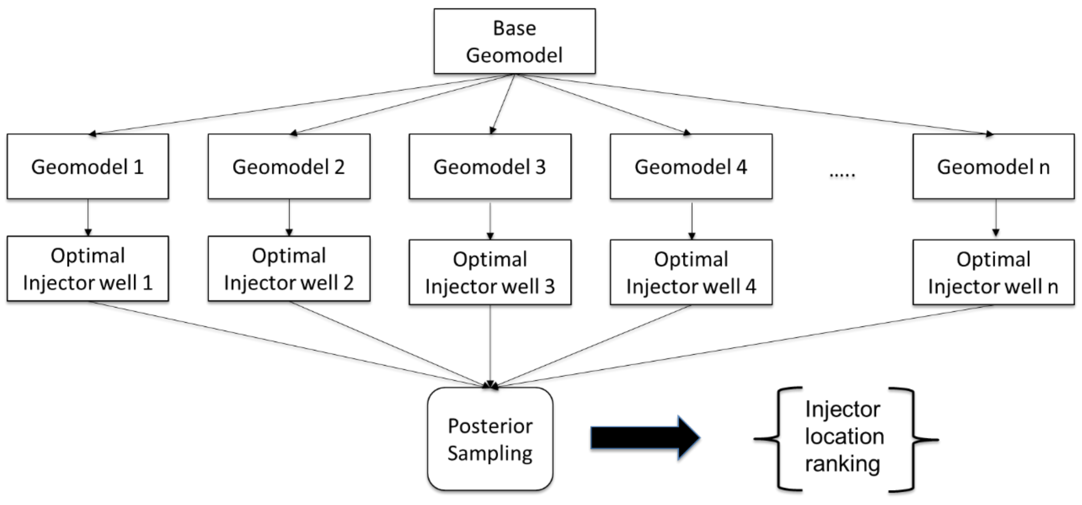
• Few studies address the selection of an optimal injection strategies from an ensemble of injection strategies arising out of geological uncertainty. Reservoir managers frequently make decisions with incomplete information. This is especially true early in the field development cycle. In the context of injection projects, the manager must decide on an injection strategy without having a complete understanding of the reservoir. For instance, there may be n number of geological realizations of a particular reservoir. Each realization may have a unique optimal injection well location; the reservoir manager may have up to n different injection locations to select. It may be computationally expensive to test each injection location on each geological realization in a brute force approach (resulting in up to n² evaluations). Posterior sampling provides an efficient evaluation approach to determine which injection strategies consistently yield higher returns across the expected range of subsurface properties.

The workflow attempts to answer the following petroleum engineering questions:

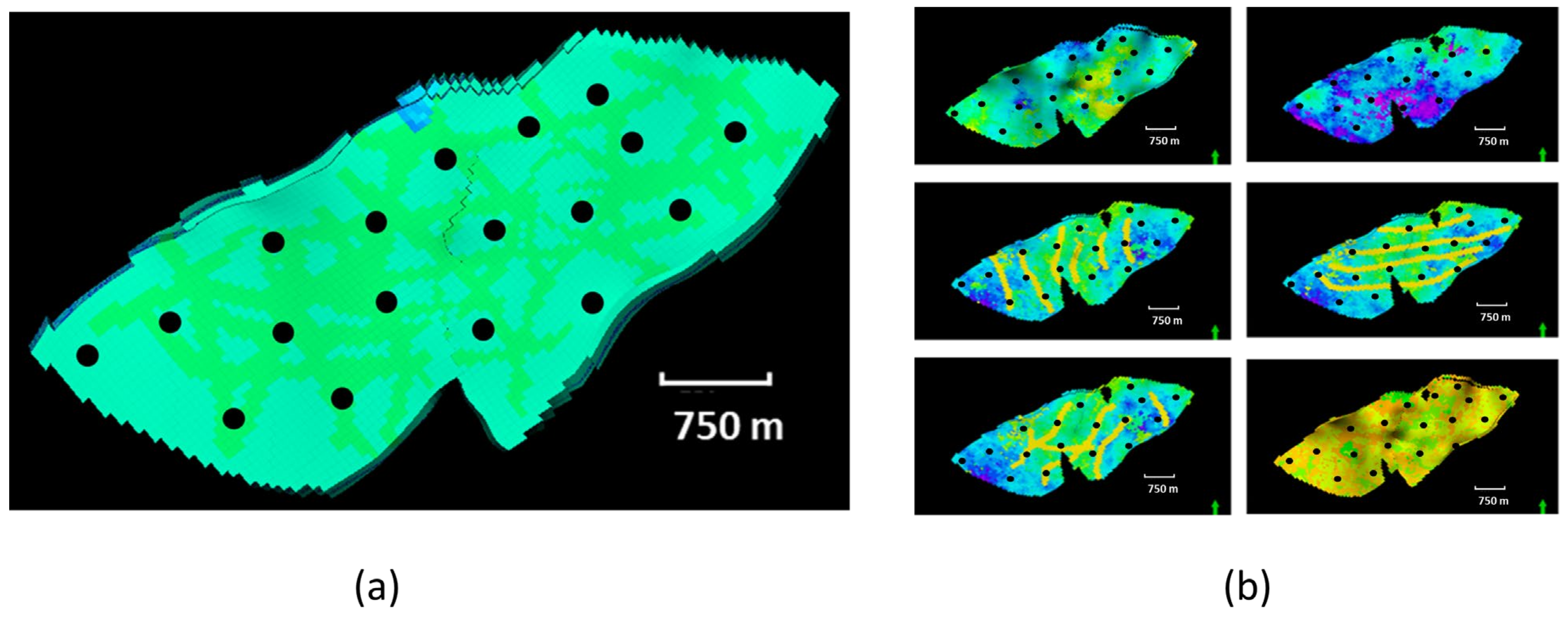
• Given existing production wells in a reservoir, where are the optimal injector locations to maximize oil recovery and/or CO₂ storage? Figure 1a illustrates this challenge: with multiple production wells (marked as black dots), where are the optimal injection locations and are there existing production wells that can be converted to injectors?
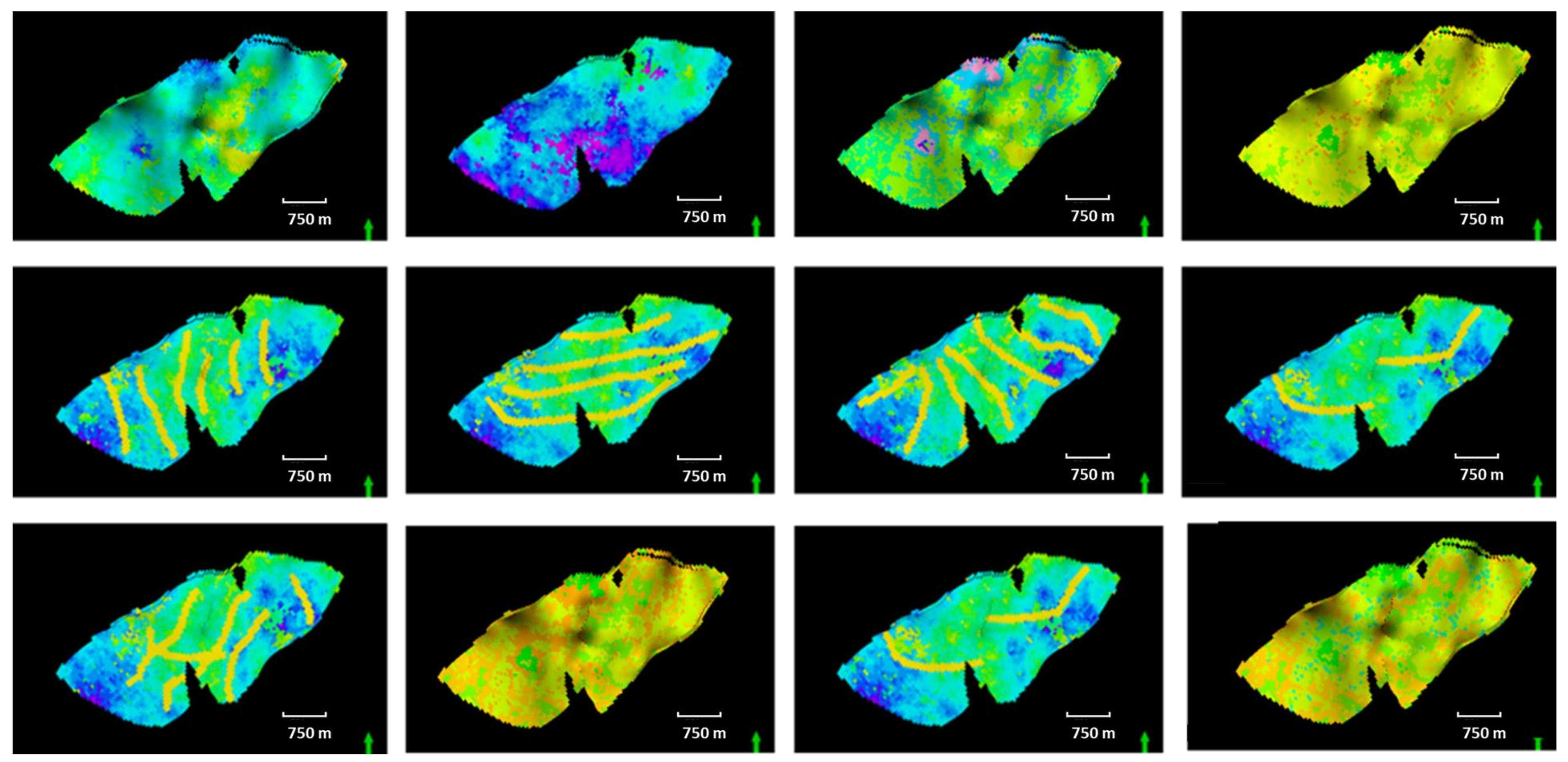
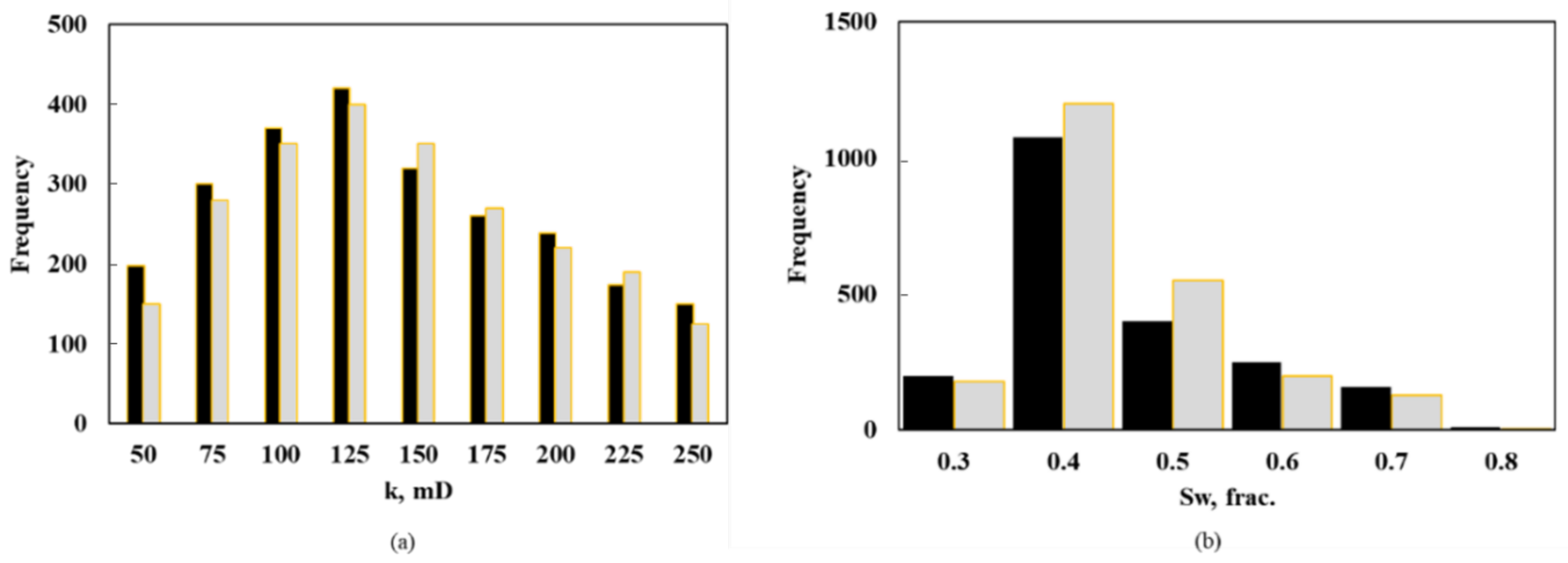
• Given a diversity of geological models and possible injection strategies, which injection strategy should ultimately be implemented? The challenge highlighted in question 1 above is compounded if there is geological uncertainty. Figure 1b illustrates a set of different geological realizations. Each realization potentially has a unique optimal injection strategy. However, one injection strategy needs to be selected for field development.

In order to answer these questions, the workflow consists of the following elements:

• A meta-learner (or Stacked learner) proxy based on a stack of models to improve accuracy.
• A novel well region concept to aggregate properties, reducing the number of potential well location evaluations.
• A streamlined simulation to reduce computational time for training dataset generation. Time-of-flight is used as a connectivity measure.
• A training dataset that consists of an ensemble of geological models to account for geological uncertainty.
• A novel posterior sampling approach to select the best injection strategy from a diverse range of injection strategies and geological realizations.

In the following section, the methodology adopted is outlined, including data generation, well region clustering, and posterior sampling. In the results section, the proposed workflow was applied to investigate injector well selection for an oilfield located in Asia. Several case studies were presented. The best locations for water injection were first investigated, followed by optimal injector locations for CO₂ EOR and storage. To validate the proxies, blind tests were conducted with geomodels not used in training. Finally, posterior sampling was implemented to obtain the best injection strategy across an ensemble of geological realizations.

2. Methodology

The proposed workflow is summarized in the following steps, and illustrated in Figure 2:

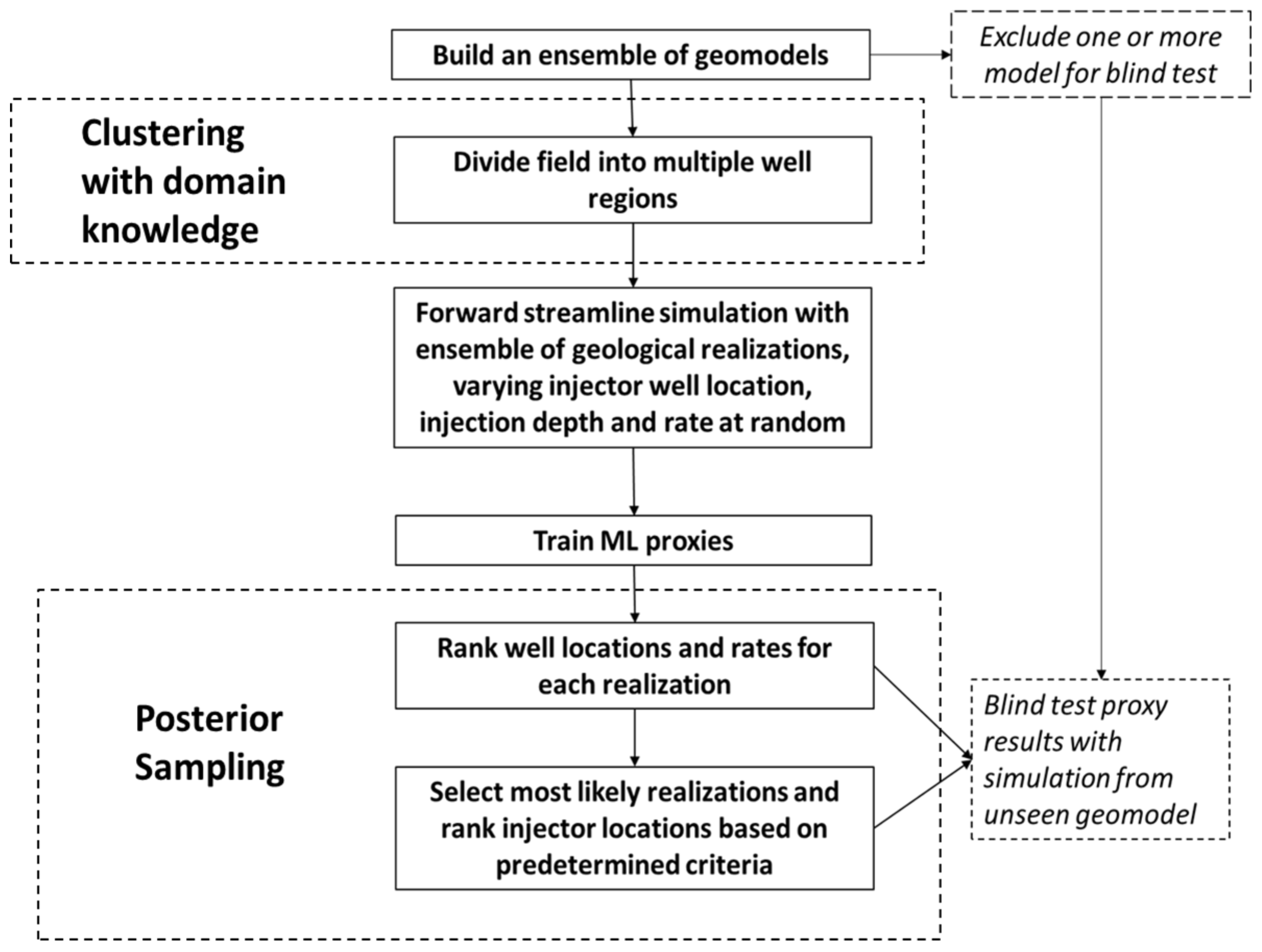
• The workflow begins with the construction of multiple geological models to capture the range of subsurface parametric uncertainty.
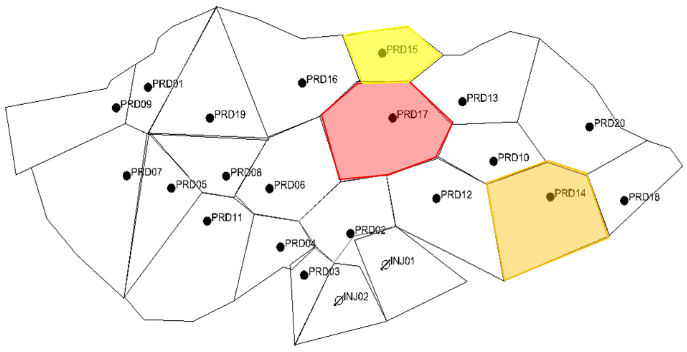
• Each geomodel is spatially divided into well regions guided by a clustering algorithm. Each region contains a single well.
• Forward streamline simulation runs are performed with the ensemble of geological models. For each run, one well is converted into an injection well. The injection depth and rate is also fixed. Each run has a unique injector well, depth and rate.
• Key geological and engineering parameters are extracted from each simulation run to build a training dataset.
• Machine Learning proxies are trained using the dataset. The proxies are trained to predict the well recoveries and/or storage potential.
• For a given geological realization, key parameters are provided to the proxy, and the injection location that maximizes certain objectives can be predicted.
• For multiple geological realizations, posterior sampling with the proxies is used to select the optimal injection locations across an ensemble of geological models.

We will describe the various elements of the workflow in the following subsections.

2.1. Data Generation

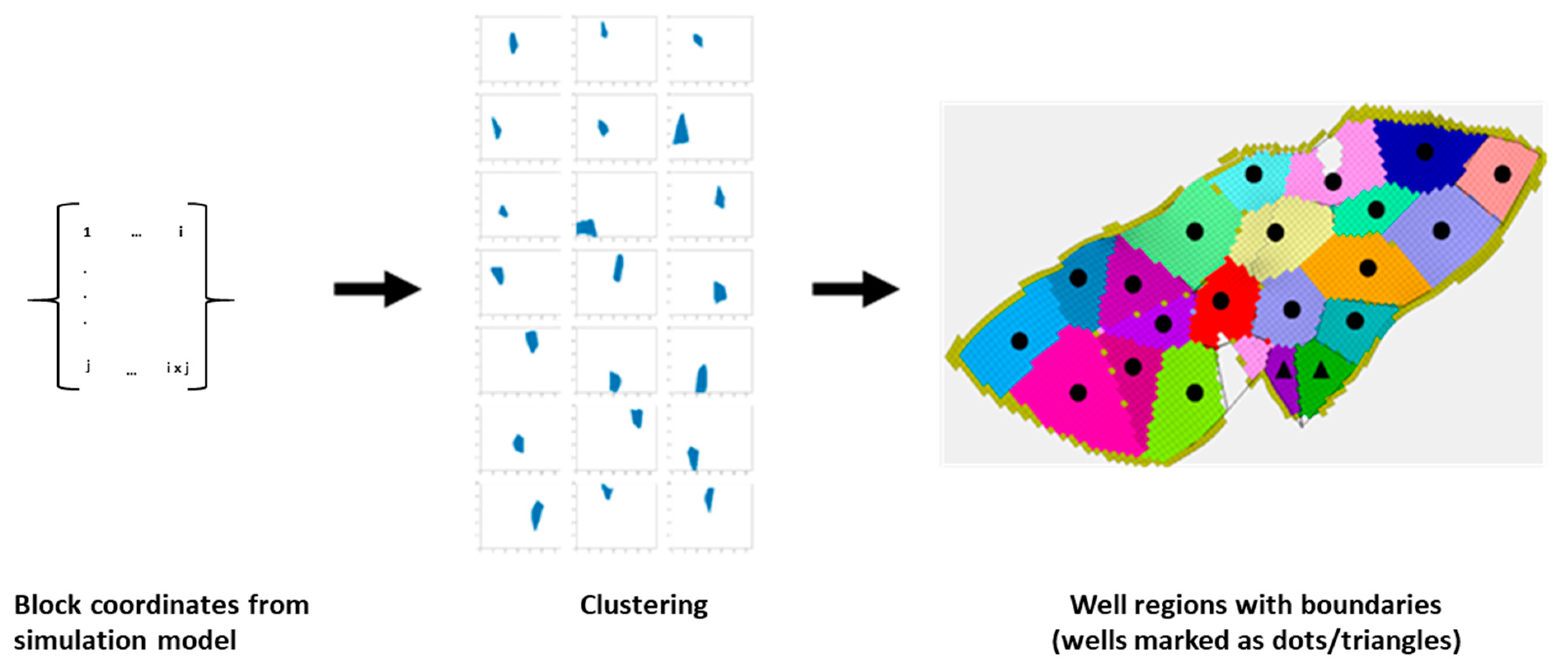
The first step of the workflow is constructing a representative set of geomodels. The field under study is currently transitioning from a primary to secondary phase. The reservoir consists mainly of fluvial-deltaic deposited sand, with reasonable permeability (mean = 150 mD) and porosity (mean = 0.22). The field had been in production for over 10 years, and the reservoir was undersaturated. Initial history matching results revealed minimal amounts of free gas. A fine-scale geological model was constructed utilizing petrophysical and geological information. Light calibration was performed to initialize the model to known fluid and rock properties. The relevant simulation properties are listed in

Table 1. Key parameters of the base geomodel.

Parameter	Value
Grid block dimensions	100 ft by 100 ft by 10 ft
Grid count	230,000
Pressure, bar	350
Average field Sw, frac	0.4
Average field porosity, frac	0.22
Average field horizontal permeability (kh), mD	150
Ratio of vertical to horizontal permeability, kv/kh, mD	0.3

. The values of pressure and saturation are the values at the end of history—this captures the current reservoir condition.

One of the challenges in developing a robust proxy is the presence of geological heterogeneities, such as multiple facies, boundaries (stratigraphic and structural), variations in permeability (both laterally and vertically) and diagenetic events [19]. These can confound attempts to map the relationship between geological parameters and reservoir responses. Well production and pressure are a complex combination of location and reservoir properties. To capture the range of possible geological realizations, an ensemble of geological models were prepared to cover a range of geological properties, with different degrees of anisotropy. These ensembles were constrained by the known petrophysical, geological and seismic data. These ensembles provided a diverse training dataset for the proxies, capturing a range of possible combinations of static and dynamic properties. In our study, we prepared an ensemble of 12 geomodels. Figure 3 shows the multiple geological realizations used for this study. Each panel is one realization; the property displayed is permeability and a variety of permeability distributions, including channel features are incorporated in each model.

With each of these models, forward simulations were conducted to generate the training and test data. Here, training data refers to the data records of features and observations used to train the proxies. The test data refers to the data records used to validate the proxies. Each data record consists of several static and dynamic parameters averaged within a defined well region. Fundamentally, the training dataset is used to ‘teach’ the proxies the relationship between the key parameters and the desired target variable; a range of different parameters were tested to understand which parameters had the biggest influence on the target variables. The features that were finally used for training were found to have an impact on prediction accuracy. The key features making up the training dataset are as follows: well region permeability, porosities, pore volumes, initial fluid saturation, pressure and time of flight. We also introduce injection depth as a feature in the training dataset. The formation is divided into three levels (top-middle-bottom) and each well can potentially inject into any of these three perforation depths. Adding the perforation depth is expected to improve the prediction, particularly with miscible gas injection. The list of features used for the proxy training is provided in

Table 2. Key features for training dataset.

Input Features		Output
Well Region Properties	Well Properties	Well Properties
Porosity	Well-to-well distances	Incremental Oil production
Permeability
Time of flight	Distance to injector
Initial water saturation
Current water saturation	Injection rate
Initial reservoir pressure
Current reservoir pressure	Injection depth
Dip angle

.

One key parameter that is tracked is the incremental oil production, shown in Equation (1),

$$\Delta N=N_{INJ}-N_{base}$$

(1)

where the incremental oil ($\Delta N$) is the difference between the oil production cumulative from the injection case ($N_{INJ}$) and the oil production cumulative from the base case ($N_{base}$). The base case cumulative is the oil production as is, meaning no further field development activities were conducted on the field. Incremental oil is an important parameter to track as it accounts for any loss in production as a result of a well conversion and captures the true value of the waterflood and/or CO₂ flood.

For the waterflooding process, a black oil model was used to capture phase behavior, using the commercial simulator FrontSim. Miscible gas injection was modelled using the pseudo-black oil model as described by Todd and Longstaff [26]. The key model parameters are presented in

Table 3. Pseudo-miscible injection parameters used for the CO₂ injection cases.

Todd Longstaff Parameters	Value
Mixing parameter, ω	0.7
Mixing exponent	−0.25
Injected gas surface density, lb/ft3	0.12

.

In all case studies, the wells were run on the same surface operational parameters as the last recorded control vectors from the history file in order to ensure consistency. For waterflooding, simulation runs were conducted under the constraints set in

Table 4. Field constraints imposed during waterflood forward modelling. The rates are in kiloliters per day (klpd).

Parameter	Value
	Lower	Upper
Field wide production, klpd	215	235
Field wide injection, klpd	215	235
VRR	0.91	1.09

. These constraints followed the operational limits determined by the operator. The injector rate was selected at random following these constraints. The training records generated by the forward simulation runs were used to train several candidate proxies. The training dataset—consisting of 12 features with 162 simulation runs—was used to train the model. To improve training performance, 10-fold cross validation was used. For each model, a total of 12 runs were made. In each run, an injector well location, injection rate and injection depth were selected at random, i.e., a single well was selected for conversion at a given perforation interval (top, middle or bottom). This was performed to ensure adequate areal and vertical coverage. Injection was performed in the selected well over a 10-year period. The injection well was run under rate control, and the production wells under bottomhole pressure control.

For the CO₂ injection cases, the simulations used the pseudo-black oil model with continuous CO₂ injection. The continuous CO₂ injection was simulated for 10 years post waterflood. The CO₂ injection rates were designed to be similar to the waterflood injection rates under reservoir conditions so that an equivalent amount of pore volume per year was injected. The selection of the CO₂ injection site was performed randomly. For each geomodel, a random well was selected six times with three possible injection depths. This yielded 216 unique injection configurations (12 geomodels × 6 wells × 3 depths). Random selection was performed to create a diverse training dataset. As with the water injection cases, the injection parameters were set following the operational constraints provided by the operator. The upper and lower pressure limits were set on the injection wells to ensure that the wells do not inject below the miscibility pressure or above the fracturing pressure. The injection parameters used for the simulation runs are provided in

Table 5. Key Injection parameters for the CO₂ injection case.

Parameter	Value
	Lower	Upper
Bottomhole pressure, ksc	265	290
CO2 Injection rate, res m3	55	75
Cumulative PV CO2 injected, %	41	45

.

2.2. Well Regions

A critical innovation of this work is to define boundaries around each well to constitute well regions. This alleviates the computational burden of multiple location evaluations mentioned in the Introduction. These well regions are akin to drainage boundaries of wells but are defined to ensure adequate coverage of the reservoir. Properties within each well region are averaged. These averaged properties constitute the training features for the proxy. If there are insufficient wells, ‘pseudo-wells’ are defined as the centroids in each region. This will ensure that the well regions are extended geometrically across the field. Well regions are delineated as follows:

• The grid block locations for each block along the mid-point surface of the reservoir of interest.
• Define the centroids of the clusters around existing wells.
• Apply the K-means algorithm [27] to cluster points around centroids, with Equation (2)

  $$\underset{c_iϵC}{\mathrm{argmin}}dist{\left(c_i,x\right)}^2$$

  (2)

  where dist(.) is the Euclidean distance, c_i is the collection of centroids in set C and x is the data-point. Therefore the points closest to the centroids are clustered using the Euclidean distance metric.
• If the data density is insufficient, the clusters will not form adjacent boundaries. Therefore, to create adjacent spatial boundaries, Support Vector Classification (SVC) [28] is applied as follows:

  a.

  The clustered data points are projected to the feature space, given by Equation (3),

  $$\varnothing \left(x_i\right).$$

  (3)

  b.

  The RBF kernel is used to transform the data following Equation (4)

  $$K\left(x_i,x_j\right)=e^{-\gamma {\left|\left|x_i-x_j\right|\right|}^2}.$$

  (4)

  c.

  The classical statement of the SVC problem is

  $$\underset{w,b,\zeta }{\min }\frac{1}{2}{w}^{T}w+C{\displaystyle \sum }_{i=1}^n{\zeta }_i$$

  (5)

  subject to $y(w^T\varnothing \left(x_i\right)+b\ge 1-{\zeta }_i$ where ${\zeta }_i\ge 0,i=1\dots n$. Here the goal is to maximize the margin (by minimizing ${\left|\left|w^T\right|\right|}^2$, with a penalty term C. The dual problem can then be stated as

  $$\underset{\alpha }{\min }\frac{1}{2}{\alpha }^T{y}_i{y}_{j}K\left(x_i,x_j\right)\alpha -e^T\alpha$$

  (6)

  subject to $y^T\alpha =0$, with $0\le {\alpha }_i\le C,i=1,\dots n$. Here, Q is a n by n positive semidefinite matrix. The terms ${\alpha }_i$ are dual coefficients bounded by C.

  d.

  The solution of the optimization problem (Equation (6)) then yields the classification function that defines the decision boundaries,

  $${\displaystyle \sum }_{i=1}^N{\alpha }_i{y}_{i}K\left(x_i,x\right)+b$$

  (7)

• The boundaries are adjusted by the user based on structural features such as faults.

An example of the clustering approach is presented in Figure 4. The grid block addresses were obtained from the simulation model and were used as a clustering parameter. The mid-point surface block addresses were clustered to yield well region boundaries. With some minor adjustments to account for faulting, well region boundaries were determined as shown in in Figure 4. Note that in this case study, the well coverage across the field was adequate—no pseudo-wells were needed.

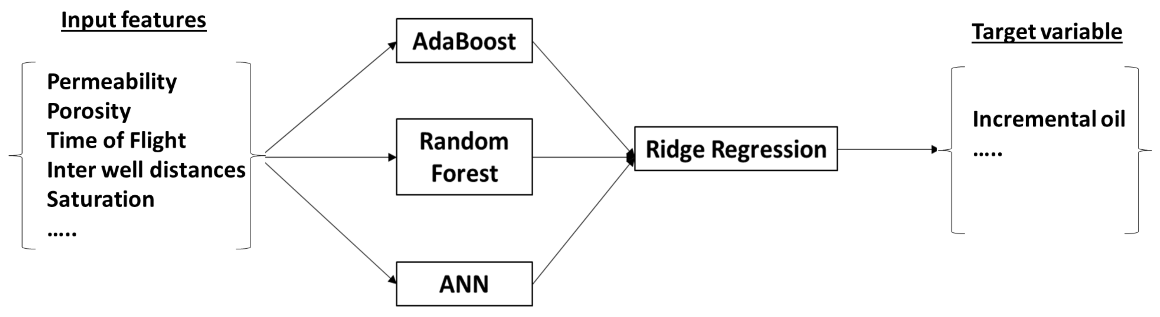
2.3. Meta-Learner Proxy

Stacking is a method of combining multiple algorithms (base learners) to form a meta-learner. The base learners could be any machine learning algorithms. The motivation behind stacking is to leverage the prediction power of each base learner to produce a more accurate prediction. Our approach to stacking is adopted from [29] and is illustrated in Figure 5 as follows:

• Training data (X) is fed into the three base learner algorithms, namely AdaBoost [30], Random Forest [31] and Artificial Neural Networks (ANN) regressor [32].
• The training dataset, X, consists of the input features (for example features listed in Table 2). Here $X\in {\mathbb{R}}^{n\times p}$, where n is the input data and p is the output, or target data).
• The dataset X is split into K- folds using k-fold cross validation. We used five folds. One fold is held as a validation set and the others used to train the three base learners. The trained models are tested on the data in the validation fold. This process is repeated so that all of the folds have been used as the validation dataset. In this manner, each data point has been used as a testing and training data point.
• The predictions from each base learner is stacked to create a matrix Z ($Z\in {\mathbb{R}}^{pxL})$ where L is the number of base learner algorithms.
• The meta learner is fitted on Z using ridge regression to minimize the following cost function,

  $$\frac{1}{2n}({\displaystyle \sum }_{i=1}^n{\left(y_i^{\prime }-y_i\right)}^2+\lambda {\displaystyle \sum }_{j-1}^p{w}_j^2)$$

  (8)

  where n are the number of training observations, y′ are the predictions from the base learners, y_i is the actual target data, w_j is the fitting coefficient and $\lambda$ is the tuning parameter.

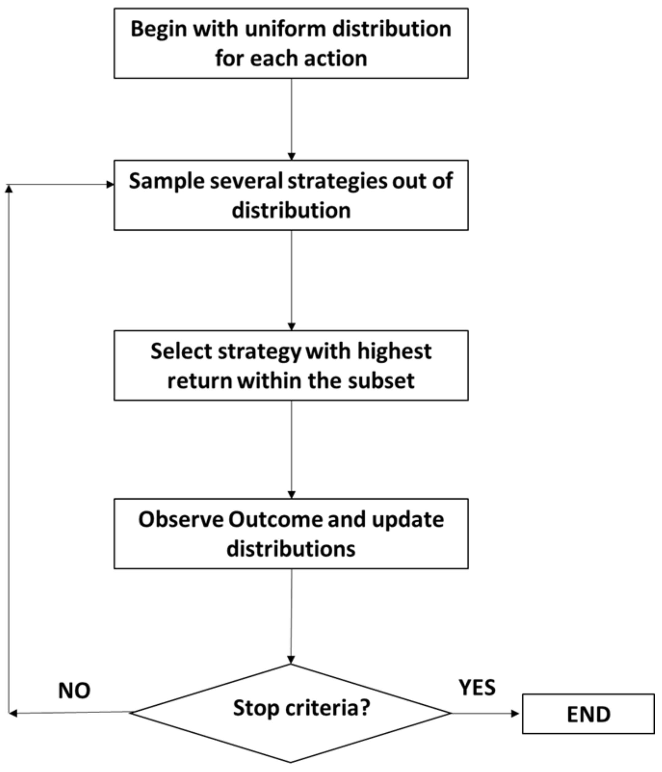
2.4. Posterior Sampling

In Section 1, the challenge of selecting an injection strategy with a geomodel ensemble was introduced. The proposed solution is to utilize posterior sampling to aid decision making under uncertainty. This approach is based on the methodology introduced by Thompson [33] for allocating experimental resources in clinical trials.

Posterior sampling begins by utilizing a prior reward distribution to indicate the probability of a reward given a certain action. This prior is updated iteratively by testing a variety of decisions and recording the rewards. The rewards can include metrics, such as profit, net present value or incremental oil production. In the early iterations, the algorithm search is broad, and every action is tested at least once. With more iterations, actions that tend to yield higher rewards are favored. Eventually the decision maker is presented with posterior probabilities of the actions and can select an optimal action. Formally, given a set of environments (X), a set of actions (A), a set of rewards (R), the key components are [34]:

• A tuple D = {(m, a, r)} where m = state, a = action, r = reward.
• A likelihood function P(r|θ, a, m).
• Model parameters (θ).
• A prior distribution P(θ).
• A posterior distribution P(θ|D) ∝ P(D│θ)P(θ).

The goal of the algorithm is to maximize the expected reward E(r|a) given by

$$\left(r|a,x,\theta \right)=ma{x}_{a^{\prime }}E\left(r|a^{\prime },x,\theta \right)$$

(9)

The initial priors for the outcome of each decision are set to be uniform. The algorithm then takes a sample (θ) from the outcome distributions P(θ|D) for each action (a) and simulates the sample with the highest reward E(r|θ, a, x). The observed outcome updates the posteriors and this process is repeated until a terminating criterion is reached. Figure 6 illustrates the algorithm process.

3. Results and Discussion

In this section, results from several key case studies utilizing the geomodel ensemble described in Section 2.1 are presented. The case studies test the ability of the proxy to capture reservoir dynamics for waterflood recovery, CO₂ flood recovery and CO₂ storage. The proxy was also tested with blind cases studies. Lastly, posterior sampling is used to select the optimal injection strategy given multiple options. In each section, the prediction results from the proxies are compared with the streamline simulation results (discussed in Section 2.1).

3.1. Waterflood Case Study

The geomodel ensemble described in Section 2 is used to generate a training dataset for the proxies. The experimental controls highlighted in Section 2.1 were used to simulate the waterflooding process, with the training features highlighted in

Table 6. Key input and output features for the waterflood proxies.

Input Features		Output
Well Region Properties	Well Properties	Well Properties
Porosity	Well-to-well distances	Incremental Oil production
Permeability
Time of flight	Distance to injector
Initial water saturation
Current water saturation	Injection rate
Initial reservoir pressure
Current reservoir pressure	Injection depth
Dip angle

. The proxies outlined in Section 2.3 were trained with a 10-fold cross validation to improve performance.

The results of the proxy modelling on the training and validation dataset are provided in Figure 7 below. A comparison between the error metrics of the different proxy models are provided in

Table 7. Summary of proxy performance and time to make predictions for 3000 samples for various proxies.

Model	R2	R	MAE	RMSE (kls)	Training Time (s)
Stacked learner	0.98	0.96	1346	6240	4.4
Adaboost	0.95	0.91	1972	6330	1.7
Random Forest	0.94	0.88	4035	9701	1.2
ANN	0.84	0.71	7098	15,012	8.1

. Several error metrics were used to compare the incremental oil production between the simulation results and the proxy results, including the R and R² values. The RMSE values are also useful, as these provide an absolute measure of the error of the proxy prediction (in kls).

Based on the results outlined in Table 7 and Figure 7, several observations can be made:

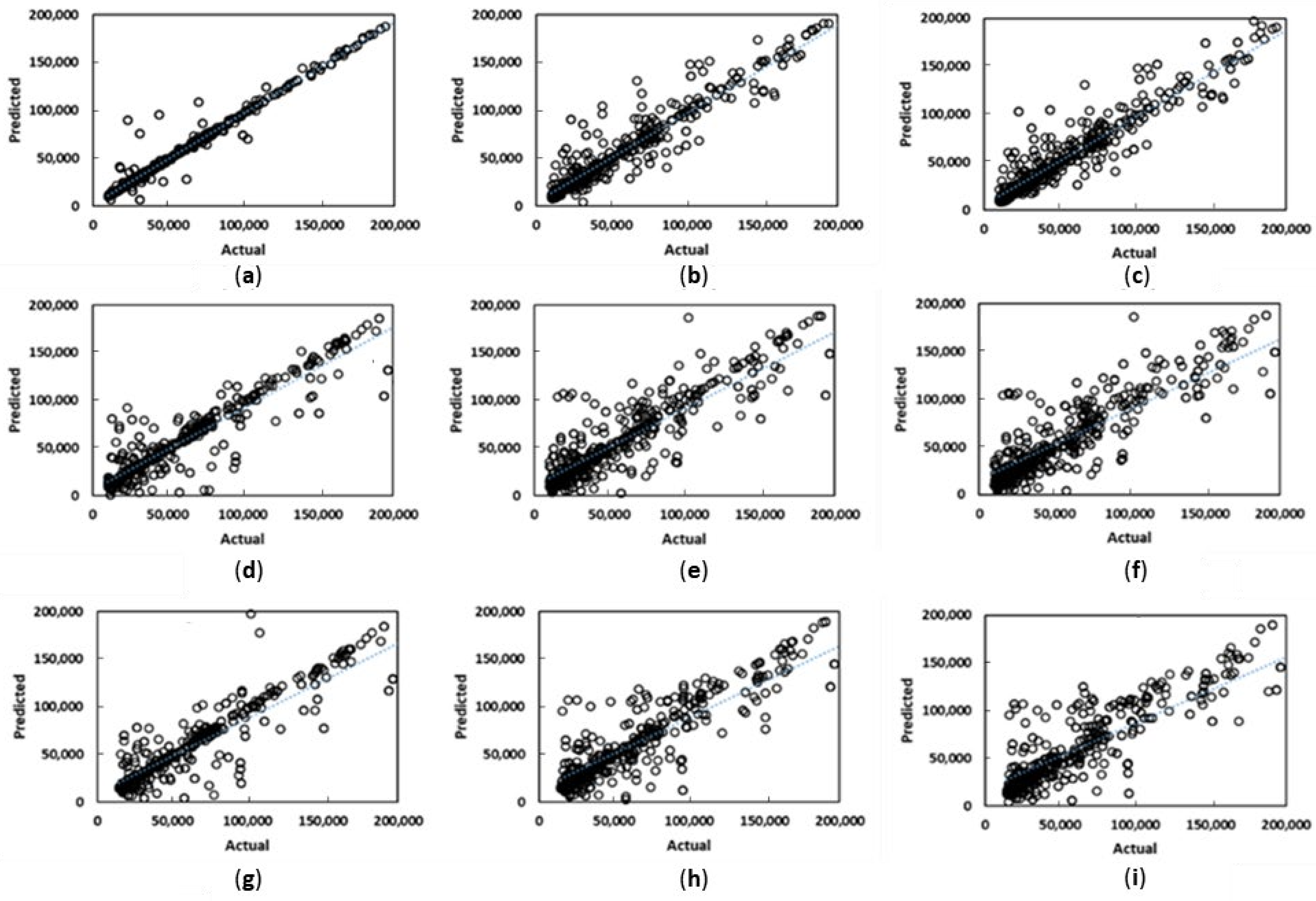
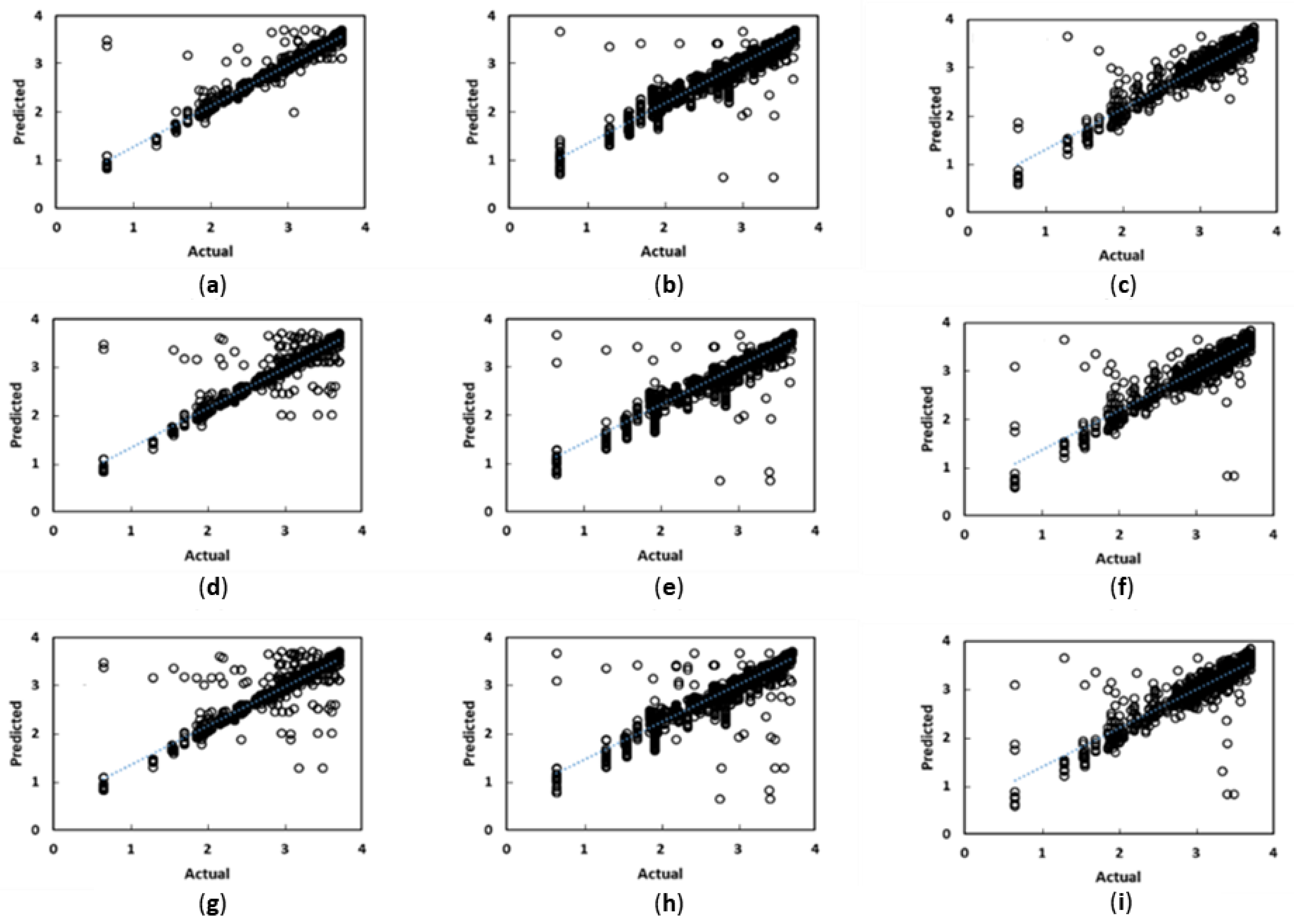
• Figure 7 compares the prediction performance for three proxies, for three training sample sizes. The prediction results from the proxies are on the ordinate and the numerical simulation results on the abscissa. The Stacked learner (combining AdaBoost, Random Forest and ANN models) performs best, highlighting the value of the meta-learner approach. The Stacked learner also had the smallest reduction in R² scores as the samples reduced. The Stacked learner had a reduction of 11% from 3000 to 1000 samples, compared to 16–18% for the other models trained.
• The proxy performance demonstrates that the training features selected are adequately capturing the relationship between geological parameters and production; however, given the variation of geological parameters, a larger number of training instances is required to obtain accurate predictions. This is demonstrated by the loss of accuracy as the number of training samples are reduced (between 11–18% reduction in R² scores).
• From Table 7, the RMSE values of the top performing model indicate that, for a given geomodel, the difference between the proxy prediction and actual values are approximately 6000 kls. With the average incremental oil of approximately 60,000, this yields a relative error of 10%. This margin of error is similar to history matching errors of oil reservoirs [35], where the calibration of numerical simulation models to observed data result in 5–20% relative error. This indicates that the predictive ability of the trained proxy is comparable to a calibrated numerical simulation model.
• The total training time for the models peaks at just above 4 s for the stacked learner. The total time taken to generate the data for training the proxies is approximately 20 h; each individual streamline simulation run takes 8 min. The time taken to evaluate the secondary phase recovery for each well location within each geological ensemble will take approximately 96 h (8 min × 12 models × 20 well locations × 3 perforation depths).

One of the distinctions of this work is the use of time-of-flight (TOF) as a training feature. TOF provides useful information about the connectivity between different well regions. To illustrate the value of TOF, a sensitivity run was conducted to eliminate the use of the TOF coordinate as an input feature. The results in Figure 8 show that the TOF coordinate plays an important role in capturing the injection-production dynamics, and inter-well connectivity. The Stacked learner R² score reduced from 0.98 to 0.87 (R score reducing from 0.98 to 0.93), the AdaBoost R² score reduced from 0.95 to 0.81 and the Random forest R² score reduced from 0.94 to 0.79; the proxies are unable to properly capture the inter region fluid movement which is critical to fluid recovery in injection projects.

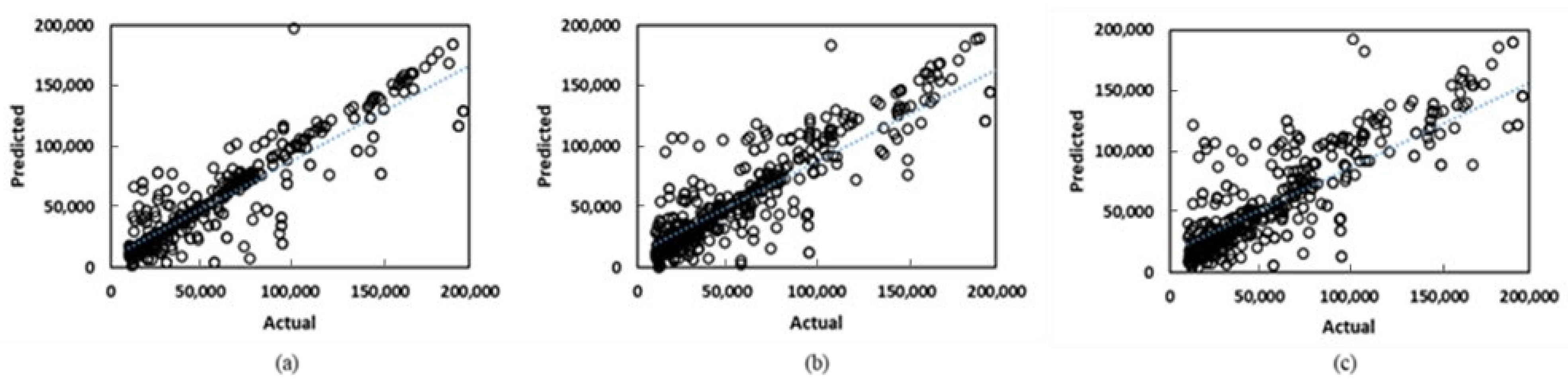
3.2. CO₂ Injection for Storage Case Study

Forward simulation runs with CO₂ injection were conducted using the geological model ensemble and simulations with the pseudo-black oil model described in Section 2. The input-output features are presented in

Table 8. Input and output features for the CO₂ storage case.

Input Features		Output
Well Region Properties	Well Properties	Well Region Properties
Porosity	Well-to-well distances	CO2 stored
Permeability	Distance to injector
Time of flight	Cumulative Oil
Initial water saturation	Perforation depth
Current water saturation	Vertical displacement between well mid-perforations
Initial reservoir pressure
Current reservoir pressure
Dip angle	Injection rate

. An additional feature was introduced to capture the vertical movement of CO₂ in the reservoir. Given the density contrast between the injected fluid and the insitu fluid, the difference between the mid-perforation depths of the injector and producers was used to capture the effect of injecting and producing from different depths. This feature addresses gravity segregation which is a common phenomenon in CO₂ injection projects [36]. Cumulative oil produced was also used as a feature to capture the effects of fluid voidage on storage capability.

The following observations can be made from the results in

Table 9. Proxy results for 3500 samples for CO₂ storage.

Model	R2	R	MAE	RMSE (bscf)	Training Time (s)
Stacked learner	0.94	0.88	0.04	0.16	10.2
Adaboost	0.9	0.81	0.06	0.18	5.5
Random Forest	0.87	0.76	0.1	0.19	2.5
ANN	0.85	0.72	0.12	0.22	12.5

and Figure 9:

• The overall proxy accuracy is reasonably close to the waterflood proxy accuracy. The Stacked learner has an R² score of 0.94 vs. 0.98 for the waterflood case. As before, the stacked proxy has an accuracy higher than that of the individual learners.
• The reduction of accuracy with lower sample sizes is similar in the CO₂ case and waterflood case. Here, the stacked learner R² scores reduce from 0.94 to 0.90 with the reduction in training samples from 3500 to 2000 samples. The accuracy loss with the stacker learner with fewer training samples is smaller than the loss with the other learners (8% vs. 11% R² score reduction). This further highlights the value of the stacked or meta learner approach.
• The RMSE score for the stacked learner is 0.16 bscf. Given the average storage of 2.8 bcf, there is a 5% relative error. The MAE scores are 0.04 bscf. This indicates that, on average, for a given prediction, the error will be 0.04 bscf, or 1% of the mean storage. This demonstrates the accuracy and reliability of the trained proxy.
• The training time for the proxies (2–13 s) is still well below the time taken to run a single numerical simulation run (20 min for the miscible injection case). The time taken to generate storage predictions for all the possible injection locations is approximately 240 h (20 min × 12 geological models × 20 unique locations × 3 injection depths). The same evaluation was performed within seconds using the trained proxy.

3.3. CO₂ EOR and Storage Case Study

The proxies were tested to recommend an injector well location to maximize both CO₂ stored and oil recovery. To combine the two metrics, a Revenue metric (Equation (9)) was defined, weighting each component equally (50% each). The weighting factor will allow the user to determine which component is more important.

$$Revenue={\alpha }_1{p}_o{Q}_{oil}+{\alpha }_2{c}_{storage}{N}_{store}$$

(10)

where p_o is the oil sale price, Q_oil is the incremental oil production from CO₂ injection, N_store is the net CO₂ stored in metric tons, c_storage is the carbon tax credit, ${\alpha }_1$ is the weighting for oil revenue and ${\alpha }_2$ is the weighting for CO₂ storage. The results for the combined metric are shown in Figure 10. The error metrics are shown in

Table 10. Error metrics for proxies with revenue.

Model	R2	R	MAE	RMSE ($mm)	Prediction Time (s)
Stacked learner	0.94	0.88	0.29	0.52	4.4
Adaboost	0.93	0.86	0.51	0.91	1.5
Random Forest	0.89	0.79	0.6	0.9	0.5

. The oil price used is $50/bl and the carbon tax is $35/metric ton.

The following observations can be made from the results in Table 10 and Figure 10:

• The overall proxy accuracy is similar to the CO₂ storage proxy accuracy. The accuracy difference between the CO₂ cases and the waterflood case is not significant (~4% difference for the Stacked learner). However, this does reflect the incresased complexity in the displacement process; the waterflood case involves immiscible displacement, whereas the CO₂ injected is miscible with the insitu oil.
• The use of the combined equation provides an opportunity for the user to incorporate the effect of the tax incentives for carbon storage. Given that the proxies can evaluate storage potential within seconds, the impact of different oil prices and carbon tax brackets can be evaluated rapidly.
• The RMSE score for the stacked learner is USD 0.52 mm. Given the average storage of USD 4.8 mm, there is a 10% relative error. As discussed in Section 3.1, this error margin is reasonable and comparable to errors from numerical simulation results.

3.4. Blind Test Case Studies

Two blind test case studies were performed to validate the trained proxy. The stacked learner proxy was tested with an unseen geomodel. This tested the ability of the proxy to generalize to a geological realization not used in the training dataset. The comparison between the geological properties of the test geomodel and the proxy training dataset is shown in Figure 11.

The proxy is first tested with a waterflood case. The output from the proxy is a ranking of injection well locations along with the expected incremental oil recovery. In order to test the validity of the proxy, forward simulation runs were conducted on the unseen geomodel to determine the best injector well location and incremental oil. These numerical simulation results form a validation set for the proxy results.

Table 11. Proxy performance on the waterflood blind test.

Proxy			Streamline Simulation
Well Name	Injection Rate	Incremental Oil	Well Name	Injection Rate	Incremental Oil
	klpd	kls		klpd	kls
PRD17	125	165,377	PRD17	125	189,948
PRD15	115	153,203	PRD12	115	166,723
PRD17	125	137,110	PRD17	125	154,656
PRD12	130	144,268	PRD12	130	151,992
PRD10	115	95,450	PRD10	115	89,381

compares the results of these runs. The well names refer to the candidate wells selected for water injection. The injection rate is designed to maintain a field voidage replacement ratio between 0.91 and 1.05.

Next, CO₂ injection was conducted on the blind test geomodel using the parameters outlined in Table 5. The input features from Table 8 were fed into the proxy and the output (CO₂ stored) was used to rank the wells; the rankings of the wells from the proxy and numerical simulation are given in

Table 12. Proxy performance compared with numerical simulation on the blind test (CO₂ stored).

Proxy			Streamline Simulation
Well Name	Depth Tag	Net CO2 Stored	Well Name	Depth Tag	Net CO2 Stored
		bscf			bscf
PRD18	3	3.55	PRD01	3	3.62
PRD01	3	3.49	PRD18	3	3.53
PRD09	3	3.22	PRD09	3	3.49
PRD20	3	3.17	PRD19	3	3.01
PRD19	3	3.11	PRD20	3	2.99

. Note that each well name represents the well region associated with that well. The time taken to evaluate the geomodel and each well location is approximately 1 min. The time taken for numerical simulation for each well location is approximately 40 min. Therefore, the total time to evaluate all well locations with numerical simulation is between 10–20 h.

Several observations can be made for the blind test results:

• The proxy rankings match the well rankings suggested by numerical simulation. These rankings indicate which locations yield higher incremental oil recovery and/or CO₂ storage when converted into injection sites (Table 11 and Table 12). Unsurprisingly, for the CO₂ injection case, the optimal injection depths are preferentially lower rather than higher. The proxies are therefore able to locate the best injection locations both areally and vertically. The rate variation in Table 11 is limited by the restrictions placed on bottomhole injection pressure and voidage replacement ratio. A potential future work is to construct a more robust proxy to incorporate a larger rate variation for both producers and injectors.
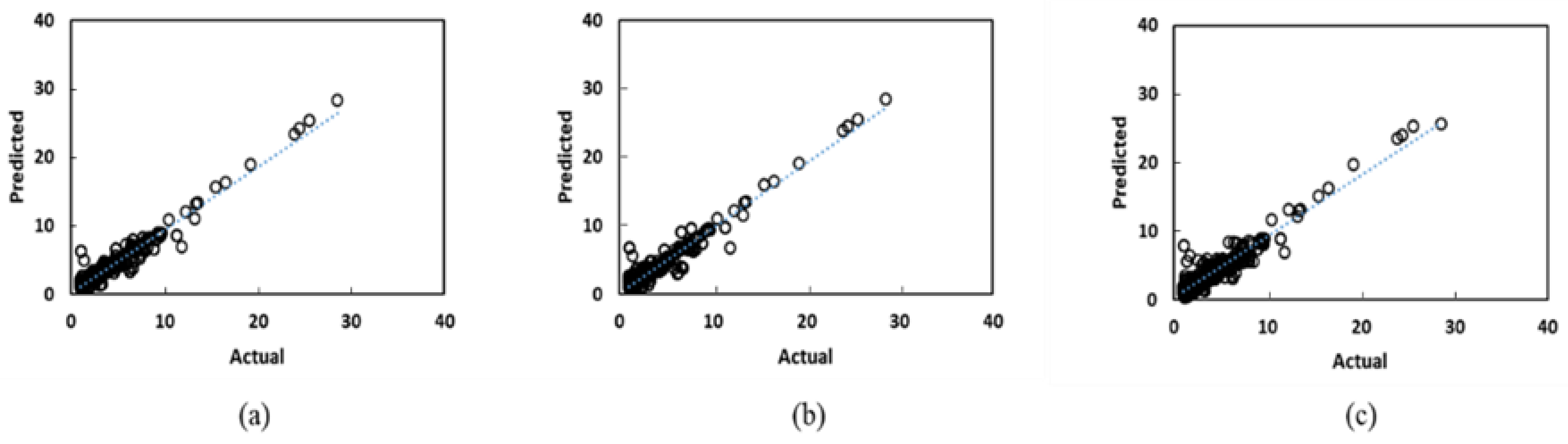
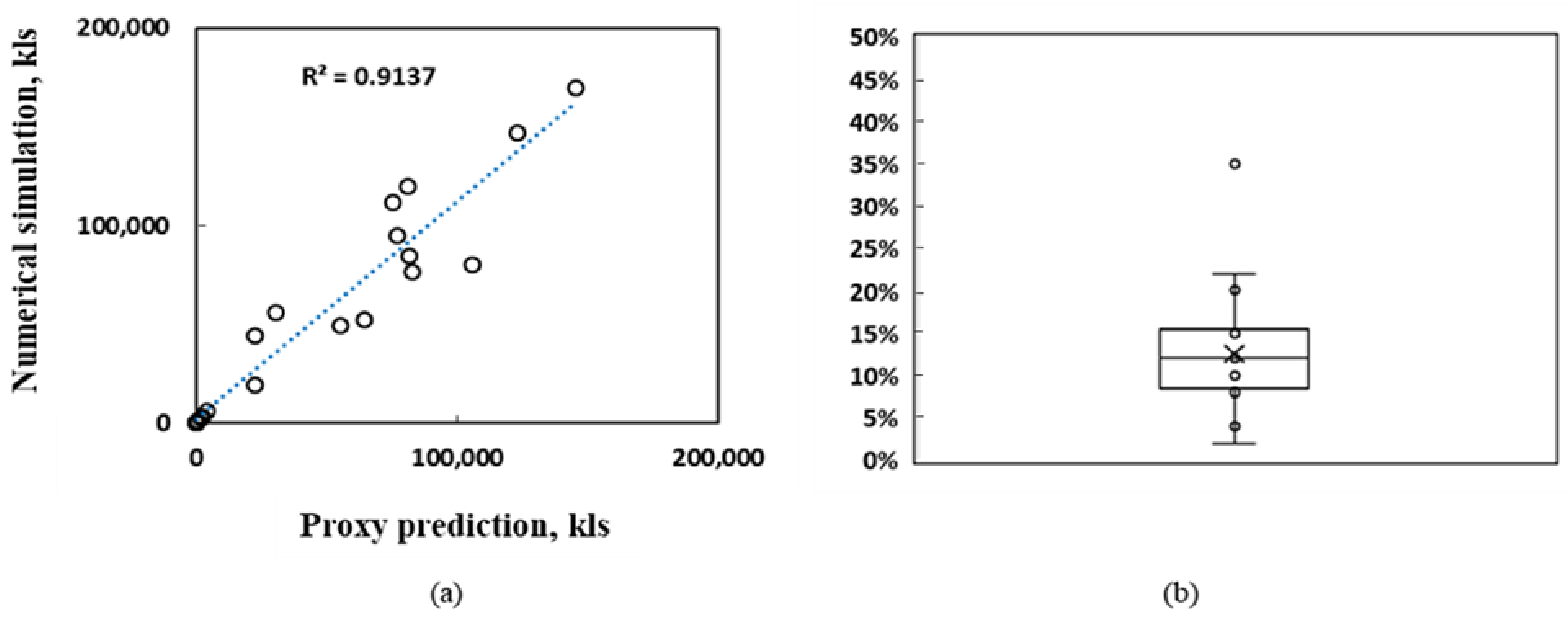
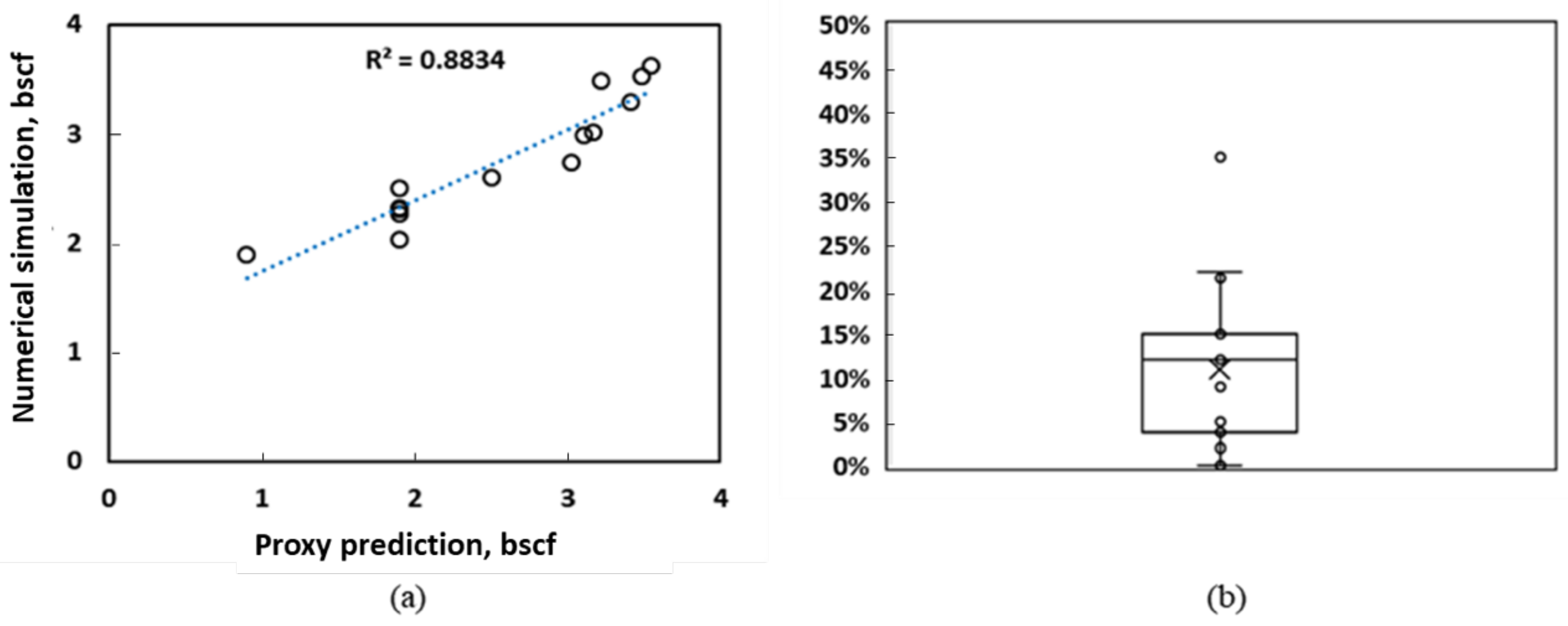
• From Figure 12a and Figure 13a, the R² values are reasonable, ranging from 0.88 to 0.91. This highlights the ability of the proxy to generalize to an unseen dataset. This is an example of a case where the proxy is trained on a subset of a geological models, and used to predict incremental oil and/or CO₂ storage potential from multiple geological realizations.
• The box and whisker plots in Figure 12b and Figure 13b indicate that the median error is 12–15%; the maximum error is 35%. As highlighted earlier, this error range is comparable to prediction errors from numerical simulation models [34]. This demonstrates that a trained proxy is able to replicate the predictive quality of expensive numerical simulations.
• Note that the well rankings, recoveries and storage potentials in Table 11and Table 12 are only valid for the geological realization tested. These rankings will likely change with different geological configurations i.e., different channel orientations and petrophysical properties. The selection of the optimal injection strategies across a range of geological realizations is discussed in Section 3.5.

3.5. Posterior Sampling to Determine Ideal Injection Location

In the previous sections, we utilized the proxies to recommend injection locations that maximize certain objectives (oil recovery, CO₂ storage and revenue). However, the optimized injection locations are unique to each geological realization. Different geological realizations may yield different injection recommendations (i.e., different injection locations). The question for the decision maker is as follows: if there are a given number of geological realizations—and each realization has an optimal injection strategy—which injection strategy should be chosen for field implementation? A brute force approach is to test all or most of the recommended injection strategies on each geomodel. Therefore, if there were 20 geomodels with 20 optimal injection strategies, a total of 400 evaluations will be required. A more efficient approach would be to use the sampling method outlined in Section 2. This is illustrated in Figure 14.

The workflow in Figure 6. Algorithm process flow for posterior sampling was implemented with the trained Stacked learner and geomodel ensemble from Section 3.1. The proxy was trained to predict incremental oil given an injection well location and rate. The posterior sampling script would select an injector well location and provide that to the proxy, along with the well region information associated with the geomodel of choice. The proxy will calculate the incremental oil from the chosen strategy with the geomodel. This process was repeated iteratively until the sampling terminates. With the 20 geomodel ensemble, well region information was extracted and used to train proxies. For each geomodel, the optimal injection location was determined using the proxy. Posterior sampling was then executed to efficiently test the various injection strategies on different geomodels and obtain a ranking of injection strategies.

The posterior sampling was run for 400 iterations. In practice, the iterations will terminate once a stopping criteria is reached. Examples of stopping criteria include imposing a predetermined number of evaluations (say 50) or setting a probability threshold for the posterior probability of any option evaluated (for instance, 90%). Figure 15 illustrates the operation of the algorithm. The initial iterations are fairly spread out between all the possible injection well locations. This is because the initial assumption is that all injection strategies have the same return—that is, the first distribution is a flat or uninformative prior. After several iterations, a few preferred candidates emerge; eventually the best candidates are selected far more often. This illustrates how the algorithm balances the exploration–exploitation trade-off. The initial search is broad, covering all of the possible strategies at least once. Subsequent iterations narrow down the possible strategies and finally converge on one. The algorithm converges to a few strategies within 30 iterations and then further narrows down to five strategies within the next 30 iterations. The probability distributions for each strategy over 400 iterations is presented in Figure 16.

From the sampling results, it is clear that a few well locations consistently emerge as the ideal locations for water injection to maximize incremental oil recovery. These are well numbers 17, 15 and 14, illustrated in Figure 17. These wells are located towards the middle of the field. It appears that injection in these locations better supports a larger number of production wells yielding higher incremental oil recovery. In order to validate the results of the posterior sampling, numerical simulation was performed with the top five well locations as injection sites. The recommended injection locations were individually simulated in each of the 20 geomodels.

Table 13. Comparison between proxy results from posterior sampling and average incremental oil from numerical simulation for the top 5 candidate injectors.

Injector	Posterior Sampling (Proxy), mmkls	Streamline Simulation (Average), mmkls
17	0.158	0.169
15	0.154	0.165
14	0.139	0.151
12	0.125	0.137
20	0.12	0.13

shows the results comparing simulation and posterior sampling incremental oil recoveries. The average values presented are the averaged incremental oil recovery over the 20 geomodels simulated.

It is clear that the posterior sampling results are able to match the simulation results reasonably well. The relative error between the posterior sampling results and numerical simulation across the five wells is between 6% and 8%. Further, the ranking of the injection locations from the proxy was also supported by the simulation results. This is consistent with the blind test results discussed in Section 3.4. The overall time taken to run each of the geomodels for the five wells was over 24 h. The time taken for the proxy to evaluate all of the injection locations across the 20 geomodels was approximately 7 min.

The results outlined above illustrate the advantages of this workflow:

• The proxy trained on a geological ensemble is able to predict reservoir responses for an unseen geomodel on a field scale. In particular, time-of-flight as a connectivity feature aids the proxies to generalize to range of petrophysical properties and channel distributions. Therefore, the reservoir manager is able use the proxy trained on a subset of geological models to predict responses for other geological realizations.
• The choice of training features also provides flexibility for proxies to be trained for a variety of flood projects. Unlike many previous methods, which are focused on one flood type, this approach is applicable for both water and gas floods, including misicble injection and CO₂ storage.
• The workflow presents methods to significantly improve the time required for decision making. The prediction time for all proxies are within 5 s compared to 20 min for a single numerical simulation run. The posterior sampling approach efficiently evaluates injection strategies without requiring excessive simulation time.

This approach has been validated for a channelized sandstone reservoir, with horizontal and vertical permeability anisotropy and multiple facies present. The workflow was also validated for both water and CO₂ floods. However, the workflow has not been validated with multiple reservoir types. Further, the rate optimization was restricted to maintaining a voidage replacement ratio of 1, honoring the constraints imposed by the field operator. Therefore, there are several key areas for future work. Firstly, this workflow can be tested with a variety of reservoir types, including unconventional and fractured reservoirs. More work can be done to extend this workflow to other reservoir types. Secondly, production and injection rate optimization can be addressed. In this work, the voidage replacement ratio was set at about one, with other pressure controls constraining the injection rates. In future work, a coupled proxy model can be trained to optimize both voidage and injection rates along with the location.

4. Summary and Conclusions

This paper has presented an innovative approach to solving a common challenge in petroleum engineering, namely optimal injector well location for both water and CO₂ floods. The proposed method resolves several hurdles to rapid field development, namely long simulation times, high number of function evaluations and decision making under geological uncertainty. The proxy performance across several case studies and blind tests demonstrates comparable performance to numerical performance in terms of prediction accuracy. However, the proxy evaluations are several orders of magnitude quicker. Furthermore, as demonstrated by the case studies, the workflow presented is flexible and able to train proxies for water and CO₂ floods with different objectives. The key highlights of this work are as follows:

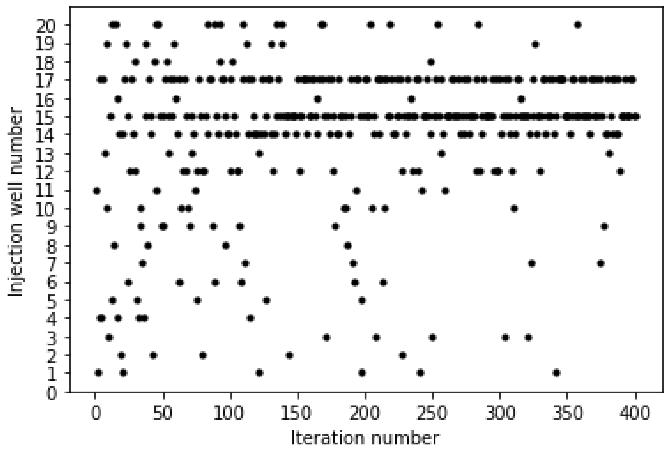
• The well region aggregation aided by machine learning is able to efficiently reduce the number of location evaluations. The field scale geomodel was reduced to 20 potential injection locations. This allows the proxies and posterior sampling algorithm to rapidly identify the areas in the field that are optimal for injection.
• The time-of-flight metric carries valuable information about the connectivity between different well regions. When this metric was removed as a training feature, the accuracies of the models reduced from an R² score of 0.98 to 0.87. Reservoir connectivity plays an important role in determining the success of an injection well. The use of the TOF coordinate as a training feature allowed the inter-well region connectivity to be described across a range of geological realizations. This was further demonstrated by the performance of the proxies on the blind tests. The proxies were able to predict with reasonable accuracies (R² scores of 0.88 to 0.91) the expected incremental oil recovery or CO₂ storage for an unseen geomodel.
• The meta-learner or Stacked proxy improves on the accuracy of individual proxies and provides robust predictions even under geological uncertainty. The Stacked proxy outperformed the individual learners by approximately 5–10% (R² scores). The accuracy reduction with fewer training samples was smaller with the Stacked learner compared to the other models; the Stacked learner R² scores reduced by an average of 10%. The other models had R² scores reduce by up to 18%.
• The use of a geological ensemble (rather than a single geomodel) provided the proxies with a diverse training dataset. This aided the proxies to generalize to unseen geomodels. The reservoir used in the case study had multiple channel configurations, with variations in key petrophysical properties. Despite this complexity, the proxy prediction accuracy on the blind tests were within 90%, comparable to numerical simulation.
• The proxies provide prediction results several orders of magnitudes quicker compared to numerical simulation. In the blind test, the time taken for the proxy to perform predictions was under ten seconds. The same evaluation would take 13 h using conventional numerical simulation.
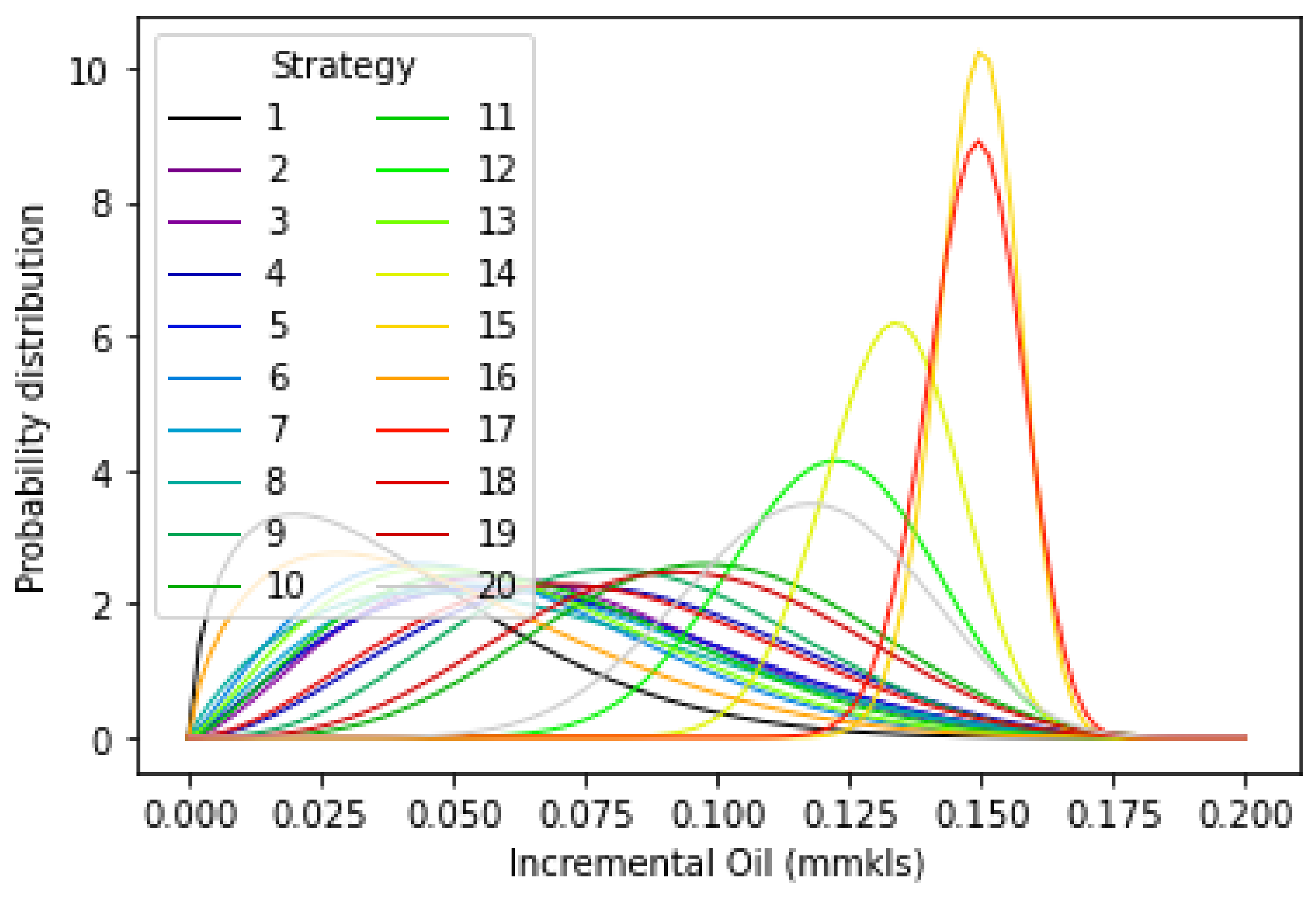
• The use of posterior sampling coupled with the proxy allows for rapid evaluations across various geomodels to decide on the optimal injection strategy without brute force evaluations. Given a geological ensemble and multiple injection strategies, the optimal injection strategy was discovered within 50–100 iterations, compared to a brute-force approach requiring 400 evaluations. When used with a proxy model, injector location evaluations can be performed under ten minutes compared to many hours using traditional numerical simulation.

References

1. Forouzanfar, F.; Reynolds, A.C. Joint optimization of number of wells, well locations and controls using a gradient-based algorithm. Chem. Eng. Res. Des. 2014, 92, 1315–1328. [Google Scholar] [CrossRef]
2. Isebor, O.J.; Durlofsky, L.J. Biobjective optimization for general oil field development. J. Pet. Sci. Eng. 2014, 119, 123–138. [Google Scholar] [CrossRef]
3. Bellout, M.C.; Ciaurri, D.E.; Durlofsky, L.J.; Foss, B.; Kleppe, J. Joint optimization of oil well placement and controls. Comput. Geosci. 2012, 16, 1061–1079. [Google Scholar] [CrossRef] [Green Version]
4. Brito, D.U.; Durlofsky, L.J. Well control optimization using a two-step surrogate treatment. J. Pet. Sci. Eng. 2020, 187, 106565. [Google Scholar] [CrossRef] [Green Version]
5. Rosenwald, G.W.; Green, D.W. A Method for Determining the Optimum Location of Wells in a Reservoir Using Mixed-Integer Programming. Soc. Pet. Eng. J. 1974, 14, 44–54. [Google Scholar] [CrossRef]
6. Güyagüler, B.; Horne, R.N. Uncertainty Assessment of Well-Placement Optimization. SPE Reserv. Eval. Eng. 2004, 7, 24–32. [Google Scholar] [CrossRef]
7. Farmer, C.L.; Fowkes, J.M.; Gould, N.I.M. Optimal Well Placement. In Proceedings of the 12th European Conference on the Mathematics of Oil Recovery, Oxford, UK, 6 September 2010. [Google Scholar] [CrossRef]
8. Wilson, K.C.; Durlofsky, L.J. Optimization of shale gas field development using direct search techniques and reduced-physics models. J. Pet. Sci. Eng. 2013, 108, 304–315. [Google Scholar] [CrossRef]
9. Litvak, M.L.; Gane, B.R.; Williams, G.; Mansfield, M.; Angert, P.F.; Macdonald, C.J.; McMurray, L.S.; Skinner, R.C.; Gregory, J.W. Field Development Optimization Technology. In Proceedings of the SPE Reservoir Simulation Symposium, Houston, TX, USA, 26–28 February 2007. [Google Scholar] [CrossRef]
10. Onwunalu, J.E.; Litvak, M.L.; Durlofsky, L.J.; Aziz, K. Application of Statistical Proxies to Speed Up Field Development Optimization Procedures. In Proceedings of the Abu Dhabi International Petroleum Exhibition and Conference, Abu Dhabi, United Arab Emirates, 3–6 November 2008. [Google Scholar] [CrossRef]
11. Janiga, D.; Czarnota, R.; Stopa, J.; Wojnarowski, P. Self-adapt reservoir clusterization method to enhance robustness of well placement optimization. J. Pet. Sci. Eng. 2018, 173, 37–52. [Google Scholar] [CrossRef]
12. Chen, H.; Feng, Q.; Zhang, X.; Wang, S.; Zhou, W.; Geng, Y. Well placement optimization using an analytical formula-based objective function and cat swarm optimization algorithm. J. Pet. Sci. Eng. 2017, 157, 1067–1083. [Google Scholar] [CrossRef]
13. Güyagüler, B.; Horne, R.N.; Rogers, L.; Rosenzweig, J.J. Optimization of Well Placement in a Gulf of Mexico Waterflooding Project. SPE Reserv. Eval. Eng. 2002, 5, 229–236. [Google Scholar] [CrossRef] [Green Version]
14. Yeten, B.; Durlofsky, L.J.; Aziz, K. Optimization of Nonconventional Well Type, Location, and Trajectory. SPE J. 2003, 8, 200–210. [Google Scholar] [CrossRef]
15. Akın, S.; Kok, M.V.; Uraz, I. Optimization of well placement geothermal reservoirs using artificial intelligence. Comput. Geosci. 2010, 36, 776–785. [Google Scholar] [CrossRef]
16. You, J.; Ampomah, W.; Sun, Q.; Kutsienyo, E.J.; Balch, R.S.; Dai, Z.; Cather, M.; Zhang, X. Machine learning based co-optimization of carbon dioxide sequestration and oil recovery in CO2-EOR project. J. Clean. Prod. 2020, 260, 120866. [Google Scholar] [CrossRef]
17. Thanh, H.V.; Sugai, Y.; Nguele, R.; Sasaki, K. Robust optimization of CO2 sequestration through a water alternating gas process under geological uncertainties in Cuu Long Basin, Vietnam. J. Nat. Gas Sci. Eng. 2020, 76, 103208. [Google Scholar] [CrossRef]
18. Thanh, H.V.; Sugai, Y.; Sasaki, K. Application of artificial neural network for predicting the performance of CO2 enhanced oil recovery and storage in residual oil zones. Sci. Rep. 2020, 10, 18204. [Google Scholar] [CrossRef] [PubMed]
19. Nwachukwu, A.; Jeong, H.; Pyrcz, M.; Lake, L.W. Fast evaluation of well placements in heterogeneous reservoir models using machine learning. J. Pet. Sci. Eng. 2018, 163, 463–475. [Google Scholar] [CrossRef]
20. Nasir, Y.; Yu, W.; Sepehrnoori, K. Hybrid derivative-free technique and effective machine learning surrogate for nonlinear constrained well placement and production optimization. J. Pet. Sci. Eng. 2019, 186, 106726. [Google Scholar] [CrossRef]
21. Aliyev, E.; Durlofsky, L.J. Multilevel Field Development Optimization Under Uncertainty Using a Sequence of Upscaled Models. Math. Geol. 2016, 49, 307–339. [Google Scholar] [CrossRef]
22. Zhang, J.; Huang, L.; Liu, M.; Cui, X.; Jiang, Z.; Bahar, A.; Pochampally, S.; Kelkar, M.G. Breaking the Barrier of Flow Simulation: Well Placement Design Optimization with Fast Marching Method and Geometric Pressure Approximation. In Proceedings of the SPE/IATMI Asia Pacific Oil & Gas Conference and Exhibition, Jakarta, Indonesia, 17–19 October 2017. [Google Scholar] [CrossRef]
23. Lyu, Z.; Song, X.; Li, G. A semi-analytical method for the multilateral well design in different reservoirs based on the drainage area. J. Pet. Sci. Eng. 2018, 170, 582–591. [Google Scholar] [CrossRef]
24. Huang, J.; Olalotiti-Lawal, F.; King, M.J.; Datta-Gupta, A. Modeling Well Interference and Optimal Well Spacing in Unconventional Reservoirs Using the Fast Marching Method. In Proceedings of the SPE/AAPG/SEG Unconventional Resources Technology Conference, Austin, TX, USA, 24–26 July 2017. [Google Scholar] [CrossRef]
25. Iino, A.; Onishi, T.; Olalotiti-Lawal, F.; Datta-Gupta, A. Rapid Field-Scale Well Spacing Optimization in Tight and Shale Oil Reservoirs Using Fast Marching Method. In Proceedings of the Unconventional Resources Technology Conference, Houston, TX, USA, 23–25 July 2018. [Google Scholar] [CrossRef]
26. Todd, M.; Longstaff, W. The Development, Testing, and Application of a Numerical Simulator for Predicting Miscible Flood Performance. J. Pet. Technol. 1972, 24, 874–882. [Google Scholar] [CrossRef]
27. MacQueen, J. Some methods for classification and analysis of multivariate observations. In Proceedings of the Fifth Berkeley Symposium on Mathematical Statistics and Probability, Berkeley, CA, USA, 21 June 1967; Volume 1, pp. 281–297. [Google Scholar]
28. Cortes, C.; Vapnik, V. Support-vector networks. Mach. Learn. 1995, 20, 273–297. [Google Scholar] [CrossRef]
29. Van der Laan, M.J.; Polley, E.C.; Hubbard, A.E. Super learner. Stat. Appl. Genet. Mol. Biol. 2007, 6, 25. [Google Scholar] [CrossRef] [PubMed]
30. Freund, Y.; E Schapire, R. A Decision-Theoretic Generalization of On-Line Learning and an Application to Boosting. J. Comput. Syst. Sci. 1997, 55, 119–139. [Google Scholar] [CrossRef] [Green Version]
31. Breiman, L. Random Forests. Mach. Learn. 2001, 45, 5–32. [Google Scholar] [CrossRef] [Green Version]
32. Rumelhart, D.E.; Hinton, G.E.; Williams, R.J. Learning representations by back-propagating errors. Nature 1986, 323, 533–536. [Google Scholar] [CrossRef]
33. Thompson, W.R. On the likelihood that one unknown probability exceeds another in view of the evidence of two samples. Biometrika 1933, 25, 285–294. [Google Scholar] [CrossRef]
34. Russo, D.; Van Roy, B.; Kazerouni, A.; Osband, I.; Wen, Z. A tutorial on Thompson Sampling. arXiv 2017, arXiv:1707.02038. [Google Scholar]
35. Sadri, M.; Shariatipour, S.M.; Hunt, A.; Ahmadinia, M. Effect of systematic and random flow measurement errors on history matching: A case study on oil and wet gas reservoirs. J. Pet. Explor. Prod. Technol. 2019, 9, 2853–2862. [Google Scholar] [CrossRef] [Green Version]
36. Han, J.; Lee, M.; Lee, W.; Lee, Y.; Sung, W. Effect of gravity segregation on CO2 sequestration and oil production during CO2 flooding. Appl. Energy 2016, 161, 85–91. [Google Scholar] [CrossRef]
Figure 1. Illustration of the injector well selection challenge for a field with existing producers (black dots) (a) and an ensemble of geological realizations (b).
Energies 14 07628 g001
Figure 2. Overall workflow proposed.
Energies 14 07628 g002
Figure 3. Geomodel ensemble used to generate training dataset.
Energies 14 07628 g003
Figure 4. Well regions (various colors) result from the clusters for the field case study, with production wells (black dots) and existing injection wells (black triangles).
Energies 14 07628 g004
Figure 5. Schematic of the meta learner used for prediction.
Energies 14 07628 g005
Figure 6. Algorithm process flow for posterior sampling.
Energies 14 07628 g006
Figure 7. Proxy results charts for incremental oil (kls) where (a) Stacked learner with 3000 samples; (b) AdaBoost with 3000 samples; (c) Random Forest with 3000 samples; (d) Stacked learner with 2000 samples; (e) AdaBoost with 2000 samples; (f) Random Forest with 2000 samples; (g) Stacked learner with 1000 samples; (h) AdaBoost with 1000 samples; (i) Random Forest with 1000 samples. The ordinate refer to the proxy predictions and the abscissa refer to the numerical simulation results.
Energies 14 07628 g007
Figure 8. Coefficient of determination charts for (a) Stacked learner, (b) AdaBoost and (c) Random Forest when the TOF is removed as a training feature. The ordinate refer to the proxy predictions and the abscissa refer to the numerical simulation results.
Energies 14 07628 g008
Figure 9. Proxy results charts for CO2 storage (bscf) where (a) Stacked learner with 3500 samples; (b) AdaBoost with 3500 samples; (c) Random Forest with 3500 samples; (d) Stacked learner with 2000 samples; (e) AdaBoost with 2000 samples; (f) Random Forest with 2000 samples; (g) Stacked learner with 1000 samples; (h) AdaBoost with 1000 samples; (i) Random Forest with 1000 samples. The ordinate refer to the proxy predictions and the abscissa refer to the numerical simulation results.
Energies 14 07628 g009
Figure 10. Proxy results charts for revenue (mm USD) where (a) Stacked learner; (b) AdaBoost; (c) Random Forest. The ordinate refer to the proxy predictions and the abscissa refer to the numerical simulation results.
Energies 14 07628 g010
Figure 11. Distribution of the permeability (a) and water saturation (b) of the training (black) and blind test (gray) dataset. The property distributions are very similar although the well level aggregations are different.
Energies 14 07628 g011
Figure 12. Blind test results using the Stacked learner proxy for incremental oil (a). The box and whisker plot (b) shows the relative error. The highest error is 35% and the median is 12%.
Energies 14 07628 g012
Figure 13. Blind test results using the Stacked learner proxy for CO2 storage (a) and box and whisker plot (b) of the relative errors for the blind test results.
Energies 14 07628 g013
Figure 14. Illustration of the diversity of injection location options with multiple geomodels and the use of posterior sampling to efficiently rank each injector location across the geomodel ensemble.
Energies 14 07628 g014
Figure 15. Well numbers selected as candidate injectors over 400 iterations through posterior sampling.
Energies 14 07628 g015
Figure 16. Incremental oil distributions for each injection location chosen after 400 iterations.
Energies 14 07628 g016
Figure 17. The top 3 well numbers recommended by posterior sampling.
Energies 14 07628 g017