Article

Dynamics and Numerical Simulation of Contaminant Diffusion for a Non-Flushing Ecological Toilet

1
National Engineering Research Center of Protected Agriculture, New Rural Development Institute of Tongji University, Shanghai 200092, China
2
State Key Laboratory of Pollution Control and Resource Reuse, College of Environmental Science and Engineering, Tongji University, Shanghai 200092, China
3
School of Mechanical Engineering, Tongji University, Shanghai 200092, China
4
Shanghai Key Laboratory of Atmospheric Particle Pollution and Prevention (LAP3), Department of Environmental Science and Engineering, Fudan University, Shanghai 200433, China
*
Author to whom correspondence should be addressed.
Energies 2021, 14(22), 7570; https://doi.org/10.3390/en14227570
Submission received: 28 September 2021 / Revised: 30 October 2021 / Accepted: 8 November 2021 / Published: 12 November 2021

Abstract

:
The poor indoor air quality (IAQ) of severely polluted toilets is associated with increased risk of severe disease. This study aimed to evaluate the overall IAQ according to the contaminant removal efficiency, volume average concentration, and breathing zone control level. The characteristics of contaminant transmission in a non-flushing ecological toilet (NFET) were analyzed using the computational fluid dynamics (CFD) methodology, and the proposed model was further validated based on experimental measurements. Both an orthogonal experimental design and CFD were used to analyze factors such as exhaust fan position (EFP), air change rate per hour (ACH), natural vent location (NVL), and grid height (G-h). The EFP and ACH were demonstrated to be the dominant factors affecting the IAQ, whereas NVL and G-h were found to play key roles. Single-factor analysis based on the significance levels of the ACH, EFP, and NVL was conducted using the CFD methodology to define three exhaust behaviors—namely, “ineffective”, “enhanced”, and “excessive”. These results provide key insights that may be used to improve the IAQ of NFETs.

1. Introduction

Restrooms, which are among the most frequently used rooms in daily life, emit large amounts of undesirable odors [1]. According to statistics from the World Health Organization, approximately 2.3 billion people worldwide lack sanitary restroom facilities, of which approximately 946 million people live without conventional restroom facilities.
Toilets contain numerous contaminants, and feces and urine produce odors as they ferment. Sato et al. [2] analyzed the malodorous volatile substances in human waste (feces and urine), and reported that approximately 90% of the malodor-causing substances are fatty acids, of which approximately 8% are N-containing compounds—including ammonia (6.5%), pyridine, pyrrole, indole, skatole, and trimethylamine. In addition, S-containing compounds (2%) such as hydrogen sulfide (1.6%) and methyl mercaptan were detected.
Various deodorization methods have been developed to deal with this problem: chemical deodorization [3], biological deodorization [4], activated sludge aeration [5], activated sludge scrubbing [6], physicochemical deodorization [7,8], and sensory deodorization, which employs aromatic and masking chemicals [9]. However, each of these solutions presents both advantages and disadvantages. Although some public restrooms have adopted air fresheners to cover odors, air fresheners have been identified as the primary source of volatile organic compounds in buildings and have the potential to damage human respiratory and immune systems [10]. Further research indicates that the presence of air fresheners, deodorants, or scented products in public toilets prevents 17.5% of the total surveyed population from using public restrooms in the United States. Hence, it is crucial to further explore ways to improve the air quality of toilets.
As ammonia and hydrogen sulfide are the most typical pollutants in public toilets [11], we investigated the odor concentration in public toilets in Shanghai by using ammonia and hydrogen sulfide detection equipment (PNT400-H2S/O3/NH3-G: Shenzhen Ruikai Lei Technology Co., Ltd., Shenzhen, China). Our findings indicated a high concentration of ammonia. Ammonia concentrations exceeding 100 mg × m−3 are sufficient to cause serious eye damage and upper respiratory tract irritation [12,13]. In addition, hydrogen sulfide is a colorless, corrosive, flammable, and toxic gas, which is both an environmental pollutant and a malodorant, with a distinctive rotten-egg smell [6,14]. Moreover, at sufficient concentrations (e.g., above 100 ppm), it is known to be a broad-spectrum poison capable of attacking several systems in the human body, including the central nervous system [15]. Exposure to 2 ppm of hydrogen sulfide can cause bronchial constrictions in asthma sufferers [16].
This study was focused on the concentration distribution and diffusion of ammonia and hydrogen sulfide in toilets. Although natural ventilation can be an energy-efficient means of improving the indoor air quality (IAQ), it is not always predictable or sufficient and may cause indoor temperatures during winter to be reported as unsatisfactory; hence, proper mechanical ventilation is essential [17]. As the prevalence of poor IAQ is a major public health concern, the control and abatement of hazardous odorants have been identified as critical tasks for maintaining adequate air quality.
Kato and Yang [18] and Novoselac and Srebric [19] used several indicators to evaluate the ventilation effectiveness. Among these indicators, contaminant removal efficiency (CRE) and breathing zone (B-Z) control level are the most commonly utilized [19,20]. Furthermore, Sandberg and Blomqvist [21] and ASHRAE [22] revealed that effective ventilation systems improve the IAQ, solving the problems of toilet odors and moist air. Computational fluid dynamics (CFD) has been applied in several studies on indoor air distribution [23,24,25,26] and pollutant diffusion [27,28,29,30]. A combination of numerical simulations and experimental measurements is typically used to analyze the ventilation effectiveness and IAQ. For example, Tung et al. [31] studied a new negative-pressure wall-type bathroom exhaust ventilation system, and performed an experiment-based analysis of the effects of the air change rate per hour (ACH) and the distance between the pollution source and exhaust vent on the distribution of the gaseous pollutant concentration in the restroom.
The main volatile substances in human waste are water soluble, and other than ammonia, these are denser than air when in a gaseous state. Tung et al. [32] introduced a local air quality index and exposure index for medical staff to evaluate the ventilation effectiveness. They performed experiments to determine the influences of various negative pressure differences on the distribution of contaminants in toilets, using sulfur hexafluoride (SF6) tracer gas instead of pollutants to study the ventilation efficiency and air exchange rate of the test room. The results showed that the ventilation system performed best when the room was maintained at −15 Pa. In a separate study, Tung et al. [33] replaced restroom contaminants with SF6 and measured the concentrations of contaminant gases in the restroom under three different ventilation modes to compare the ventilation efficiencies of these modes. The results showed that indoor contaminant concentration was lowest when the ventilation system that combined air supplies from the ceiling of the house and side wall exhaust was adopted.
Non-flushing ecological toilets (NFETs) are environmentally friendly toilets that do not require a sewer but directly collect feces and urine to a collection tank and conduct harmless treatment [34]. The benefits of non-sewered onsite sanitation systems are increasingly being recognized [35]. These are in great demand at construction sites, in remote areas, at Fangcang Hospital, in drought-affected areas, and in other areas where sewer systems are not available [36]. It can achieve the main aim of sanitation: protecting public health and the environment [37].
In addition, because NFETs reduce the water and wastewater flows within buildings, the United States Green Building Council has used NFETs to achieve leadership in energy and environmental design certifications [38]. Although several studies have been conducted on the diffusion of contaminants in private restrooms, hospital wards, and flushing toilets, limited studies have been conducted on the odor diffusion dynamics of NFETs.
Conventional ventilation systems in public restroom feature small exhaust fans, typically mounted in the ceiling or wall of the restroom, which extract unpleasant odors through the exhaust ducts. However, a greater ACH is required for systems with longer contaminant diffusion paths; in such cases, the concentration of contaminants in the immediate vicinity of restroom users is higher, and the wind speed in the restroom becomes too high, with a noticeable blowing sensation affecting the indoor comfort levels.
In this study, we used a combination of numerical simulations and experiments to study the odor concentration reduction in NFETs, to improve the air quality. The water-free ecological toilets considered in this research represent a departure from traditional toilets in several aspects. For example, although the pollutants in traditional toilets diffuse from the toilet location, those in the NFETs considered in this study diffuse from the surface of the fermentation tank. The manure produces pollutants, such as ammonia and hydrogen sulfide, during the fermentation process. Several previous studies have considered the influence of the ACH on the pollutant removal efficiency; however, the effects of air inlet and outlet positions on the pollutant diffusion dynamics are often overlooked. Therefore, we performed orthogonal experiments to study the effects of different factors on the IAQ of NFETs. In particular, we focused on the influences of the ACH, exhaust fan installation position, and air inlet position and height.

2. Methods

2.1. Physical Model

Figure 1 illustrates the configuration of the test bench adopted in this experimental study, which measured 0.96 m (length) × 0.96 m (width) × 2.2 m (height), and the pollution source measuring 0.5 m (length) × 0.2 m (width), where the length, width, and height correspond to the x-, y-, and z-directions, respectively. Representative odor-release experiments were performed on the pollution source. The assumptions and simplifications involved in this study are as follows. (1) The effects of differences between indoor and outdoor temperatures on the contaminant diffusion process were not considered. (2) Pollutants diffuse uniformly from the surface of the pollution source at a constant rate. Monitoring points for collecting the experimental data were placed above the center of the cubicle (see Figure 1a).

2.2. Tracer Gas Release and Measurement

We selected SF6 as the tracer gas because it has properties similar to those of the main volatile substances in human waste, being colorless, soluble in water, and denser than air. Under normal conditions, SF6 is non-toxic and non-flammable, rendering it perfectly safe. In addition, it is commonly used as a tracer gas in short-term experiments to determine the ventilation efficiencies of buildings and indoor enclosures.

2.3. Data Acquisition Equipment

An XLA-BX-SF6 portable SF6 gas detector was selected to monitor the behavior of the tracer gas during the experiments (Figure 1d). The detector was equipped with new original imported sensors and a 32-bit low-power processor, which included a circuit based on four-layer wiring to enhance its performance against weak signals and interference. In addition, it featured a built-in high-performance suction pump, stable flow rate, and switchable control based on an independent high-precision imported chip with a unique signal processing algorithm, which resulted in accurate and stable measurements. The XLA-BX-SF6 detector (Shenzhen Bridgecom Electronic Technology Co., Ltd., Shenzhen, China) had an error of ±0.01 ppm, with data recorded every 30 s for a duration of 45 min at each measurement point.
A PNT400-H2S/O3/NH3-G portable ammonia and hydrogen sulfide gas detector was used to detect the concentration of pollutants in public toilets with a resolution of 0.001 ppm (Figure 1e).

2.4. Validation of the CFD Simulation Method

CFD modeling enables efficient analysis of different configurations under various conditions. However, CFD modeling cannot replace experimental methods, as experiments are necessary to support the CFD modeling as benchmark tests [39,40]. Experiments were conducted in the school laboratory of Tongji University, using the measurement point locations indicated in Figure 1a. The laboratory was ventilated prior to the experiment to ensure that the results would not be distorted by any residual SF6 gas.
The fluid dynamics of the system were simulated using ANSYS Fluent, to determine details such as the concentrations of the various contaminants. For the simulations, the component transport model was adopted for the contaminant inlet. The standard, RNG, realizable, and low-Re k-ε models were used to simulate the gas turbulence [28,41,42,43,44]. These models consider the natural buoyancy-driven convection during the diffusion process and use the finite volume method and pressure-velocity coupling format of the SIMPLEC algorithm to obtain the discrete solution of the control equation. The CFD model was built according to the conditions applied in the experiments (Figure 1). An unstructured computational grid of polygon elements with a mesh quantity of 1.09 million, which was refined at the relevant zone, was used; it was chosen after independent verification (see Figure 2a).
As shown in Figure 2b, the results of the CFD simulation were compared with the experimental data collected under identical conditions at each monitoring point. The results obtained using the standard k-ε model were rational, revealing maximum and minimum disparities of 10% and 4%, respectively. Overall, Figure 2b shows a close agreement between the experimental and simulation data, indicating that the proposed model is suitable for predicting the distribution of indoor contaminants.
The standard k-ε model agrees well with the experimental data and has been widely adopted [45,46,47]. Therefore, considering the model performance, the standard k-ε model was selected for use in this study.

2.5. Boundary Conditions

The following boundary conditions were adopted in our simulations [11,48]: the exhaust outlet was set in accordance with the velocity outlet boundary conditions (velocity outlet); the grid and window were set as pressure inlets (pressure inlet); the walls and partitions comprising the restroom were defined as wall; the pollution source was set as mass flow outlet; and the ammonia release concentration and hydrogen sulfide release concentration were set to 2.5 × 10⁻⁷ kg/s and 6 × 10⁻⁸ kg/s, respectively [11,48].
A polygon element grid, which is an unstructured computational grid, was applied. Grid independent verification was conducted for different mesh numbers, namely, 1,840,000, 2,330,000, 3,130,000, 3,930,000, and 7,080,000. There was no significant change in the pollutant concentration for mesh numbers above 2,330,000. To enhance calculation efficiency and accuracy, a mesh number of 2,330,000 was therefore chosen (Figure 2c). The iterative calculations continued until a prescribed relative convergence of 10−6 was satisfied by all the field variables.

3. Case Descriptions

3.1. Preliminary Study

Figure 3a illustrates the configuration of the restroom model adopted in this study, which measured 1.85 m (length) × 1.24 m (width) × 2.95 m (height) and included a fermentation tank measuring 0.8 m (length) × 0.7 m (width) × 0.5 m (height), where the length, width, and height correspond to the x-, y-, and z-directions, respectively.
Airflow movements in NFETs are so complex that it is difficult to study a number of influential factors simultaneously. Thus, a preliminary investigation is necessary.
As demonstrated in a previous study [31], the exhaust fan position (EFP) is an important factor with regard to contaminant removal. To obtain a deep insight into the influence of the EFP, two sets of cases were designed with different EFPs (see Figure S2: Case 1-F (0,0.62,0.59), Case 2-F (0.07,0.62,0.85)), unit: m. The pollutant concentration variation with height was studied at five points A, B, C, D, and E (see Figure 3c). National standards stipulate that the ACH should be greater than 5 h−1 (GB/T 17217−1998 for urban public toilets, CJJ 14−2016) [49,50], and 10−15 h−1 (National Civil Building Engineering Design Technical Measures HVAC Power) [51]. Therefore, in our preliminary research, air supply rates of 5 h−1, 10 h−1, 15 h−1, and 20 h−1 were selected. The concentration standards for ammonia and hydrogen sulfide in public toilets are shown in Table 1 [49].
The ACH clearly affects the contaminant concentrations, which gradually decrease with increasing ACH. The contaminant concentrations along the vertical lines are shown in Figure 4, and Figures S3–S6. Figure 4a,b show the changes in ammonia concentration as functions of the ACH and height, respectively, whereas Figure 4c,d depict the corresponding plots for varying hydrogen sulfide concentration.
As shown in Figure 4a, at an ACH of 5 h−1, the ammonia concentration decreases slowly as the height increases, before stabilizing. At an ACH of 10 h−1, it is concentrated between 0 m and 0.5 m. Within this zone, the ammonia concentration decreases rapidly with increasing height. In contrast, between 0.5 m and 2.2 m, the ammonia concentration first increases, stabilizes, and then decreases.
As the ACH is increased to 15 h−1 and 20 h−1, the ammonia concentration approaches 0 between the heights of 0.5 m and 2.2 m. The variation of the hydrogen sulfide concentration follows similar trends, as depicted in Figure 4c.
As shown in Figure 4b, at an ACH of 5 h−1, the ammonia concentration decreases rapidly as the height increases from 0 m to 0.1 m. Above this height, the ammonia concentration tends to 0 mg × m−3. Moreover, when the ACH increases to 10 h−1, 15 h−1, and 20 h−1, the contaminant concentration tends to 0; as shown in Figure 5d, the maximum hydrogen sulfide concentrations for these ACH values at the measurement locations are less than 8 × 10⁻⁵ mg × m−3. The ammonia concentrations along the vertical lines normal to the corners of the rectangle ABCD in Cases 1 and 2 are presented in Figures S3 and S4, respectively, and the corresponding hydrogen sulfide concentration measurements are provided in Figures S5 and S6, respectively. Along these vertical lines, the contaminant concentration varies with the ACH in a similar manner to that observed along the vertical line at point E. At an ACH of 5 h−1, the contaminant concentration is relatively high in both cases. In response to increasing the ACH to 10 h−1, the ammonia concentration increases only in Case 1. For ACH values exceeding 10 h−1, the contaminant concentrations are relatively low in both cases. As shown in Figure 5 and Figure 6, for the equivalent ACH values, the contaminant concentrations in Case 2 are much lower than those in Case 1, indicating that the CRE is higher in Case 2. Figure 7 and Figure 8 also indicate that Case 2 results in more effective contaminant removal, showing that vortices are generated in the restroom when the ACH is 10 h−1.
When the exhaust fan was installed under the side of the toilet, the pollutant concentrations were the lowest. Figure 8 exhibits the contours representing the mean age of air at different cross-sections. In general, the age of air is defined as the elapsed time since an air element entered the room. The distribution of the mean air age can reveal the airflow direction on the basis that air always moves from locations with lower air ages to locations with higher air ages. Thus, the air age can be used to evaluate an entire room. In addition, as the air freshness reflects the ability of the room to remove pollutants, it is widely used as an evaluation index for measuring IAQ.
At an ACH of 5 h−1, the air age in Case 1 is higher, meaning that the contaminants exist for a longer time in the restroom. In Case 2, the air age increases with increasing ACH, indicating that the ACH is larger than necessary, inducing eddy currents that affect the contaminant diffusion. The research results in this section show that the pollutant removal effect is good when the exhaust fan is installed in the lower part, which paves the way for further research.

3.2. Orthogonal Experimental Design

For maximum efficiency, we designed our study to provide comprehensive testing while minimizing the number of experiments required. Typically, experiments are designed according to either orthogonal or uniform methodologies, with the former based on the equilibrium distribution theory.
In recent years, orthogonal experimental design (OED) has gained popularity in many research areas as an approach for optimizing the system performance [42], and is a reliable and representative method. Specifically, researchers have used the OED to explore the relationships between the experimental factors and related indicators, such as the CRE and volume average concentration (VAC). In this study, we adopted the OED to analyze the ACH, EFP, natural vent location (NVL), and grid height (G-h). As shown in Figure 7, when the number of air changes increases from 3 h−1 to 4 h−1, the ammonia concentration drops sharply. Based on the results presented in Section 3.1, the ACH values of 3.5 h−1, 4 h−1, 5 h−1, and 6 h−1 were selected, and exhaust fans were positioned below the fermentation tanks F1, F2, F3, and F4. Furthermore, the values of 50, 100, 200, and 300 mm were chosen for G-h, and natural vents were positioned at L1, L2, L3, and L4 (see Figures S1b and S3a). An L16(45) orthogonal experiment was performed to determine the effects of various factors on the IAQ by enabling multifactor testing with the minimum number of experiments. The orthogonal test schemes are listed in Table S1.
Simulations were designed to consider the CRE and VAC with various factors and levels. Analyses of range and variance were performed on the collected data to identify the orders of magnitude of these factors. The full details of the calculation process employed are provided elsewhere [52].

3.3. Evaluation Index

To conduct a comparative analysis of the different ventilation strategies, the normalized values of contaminant concentration and ventilation effectiveness were used in the analysis.
The CRE evaluation index is expressed as
C R E = C e C i n C C i n
where Ce, Cin, and C represent the contaminant concentrations at the exhaust outlet and air supply outlet and the average concentration in the immediate environment, respectively.

4. Results and Discussion

4.1. Orthogonal Significance Analysis of Relevant Factors

As shown in Figure 9, the orthogonal experiments indicate that the ACH, EFP, and NVL are statistically significant factors affecting the CRE and VAC, whereas G-h is less influential. The F-value calculation results are as follows: F0.01(3,6) = 9.78, F0.05(3,6) = 4.76, F0.1(3,6) = 3.29; F0.01(3,12) = 5.95, F0.05(3,12) = 3.49, F0.1(3,12) = 2.61; F0.01(3,15) = 5.42, F0.05(3,15) = 3.29, F0.1(3,15) = 2.49.
The results of the orthogonal experiments clearly demonstrate that ACH is the dominant element determining the VAC: when the ACH increases from 3.5 h−1 to 6 h−1, the VAC values for ammonia and hydrogen sulfide decrease by 41% (Figure S7) and 37% (Figure S8), respectively. The second most influential factor is the EFP, with the VAC of ammonia decreasing by 14.7% from F4 to F1 (Figure S7), whereas the hydrogen sulfide VAC decreases by 8% (Figure S8). However, the significances of the ACH and EFP are reversed with respect to the CRE, with the EFP emerging as the dominant element. In response to changing the exhaust fan from F4 to F1, the ammonia removal efficiency increases by 1.3% (Figure 10), whereas the hydrogen sulfide removal efficiency decreases by 7.2% (Figure S9). As the next most influential factor, increasing the ACH from 3.5 h−1 to 6 h−1 results in the ammonia and hydrogen removal efficiencies decreasing by 1.2% (Figure 10) and 6.4% (Figure S9), respectively. Therefore, contaminant type should be considered when positioning the exhaust fan.
Figure 9 shows the significance of a few elements, including the NVL and G-h. The NVL is statistically significant, with a p-value < 0.05 (see Figure 9a,b): changing the NVL from L1 to L2 results in the VAC and CRE of ammonia decreasing by 12.7% and 0.6%, respectively; and changing the NVL from L3 to L2 causes the VAC and CRE of ammonia to decrease by 11.6% and 1.9%, respectively. The G-h is statistically significant (p-value < 0.05) in Figure 9a, but not in Figure 9b. In addition, whereas the NVL is statistically significant (p-value < 0.1) in Figure 9c,d, the G-h is not. As demonstrated in Figure 9, for ammonia, the factors can be ordered from most to least influential as EFP > ACH > NVL > G-h. Regarding hydrogen sulfide, the order of significance is ACH > EFP > NVL > G-h. According to previous research, the sequence of these factors regarding contaminants is EFP > ACH > NVL > G-h.
The factors examined in this study have different effects on ammonia and hydrogen sulfide because these two pollutants have different concentrations and obey different diffusion characteristics. Ammonia is less dense than air and has a higher diffusion rate, meaning that it diffuses to the upper part of the toilet more easily. In contrast, hydrogen sulfide gas is denser than air and has a slower diffusion rate, meaning that it tends to be deposited in the lower part of the toilet. The farther the exhaust fan is from the pollution source, the easier it is to extract and eject ammonia; however, the result differs in the case of hydrogen sulfide, with the ACH having a greater impact on its removal.
In short, the ACH and EFP are the most influential factors affecting the distributions of ammonia and hydrogen sulfide, respectively. Therefore, we focused on the effects of these two factors on the pollutant diffusion.

4.2. Single-Factor Analysis

After the ACH and EFP, the orthogonal experiments identified the NVL as the third most important parameter affecting the CRE and VAC. As each of these factors affects the CRE and VAC in different ways, identifying the interactions among the ACH, EFP, and NVL is key to understanding the effective use of exhaust fans for contaminant removal. Therefore, we conducted single-factor analyses for the ACH and EFP, with the G-h fixed at 300 mm and the natural vent height fixed at 2050 mm. The observation plane was located in the middle of the restroom (see Figure S1b in the Supplementary Materials).

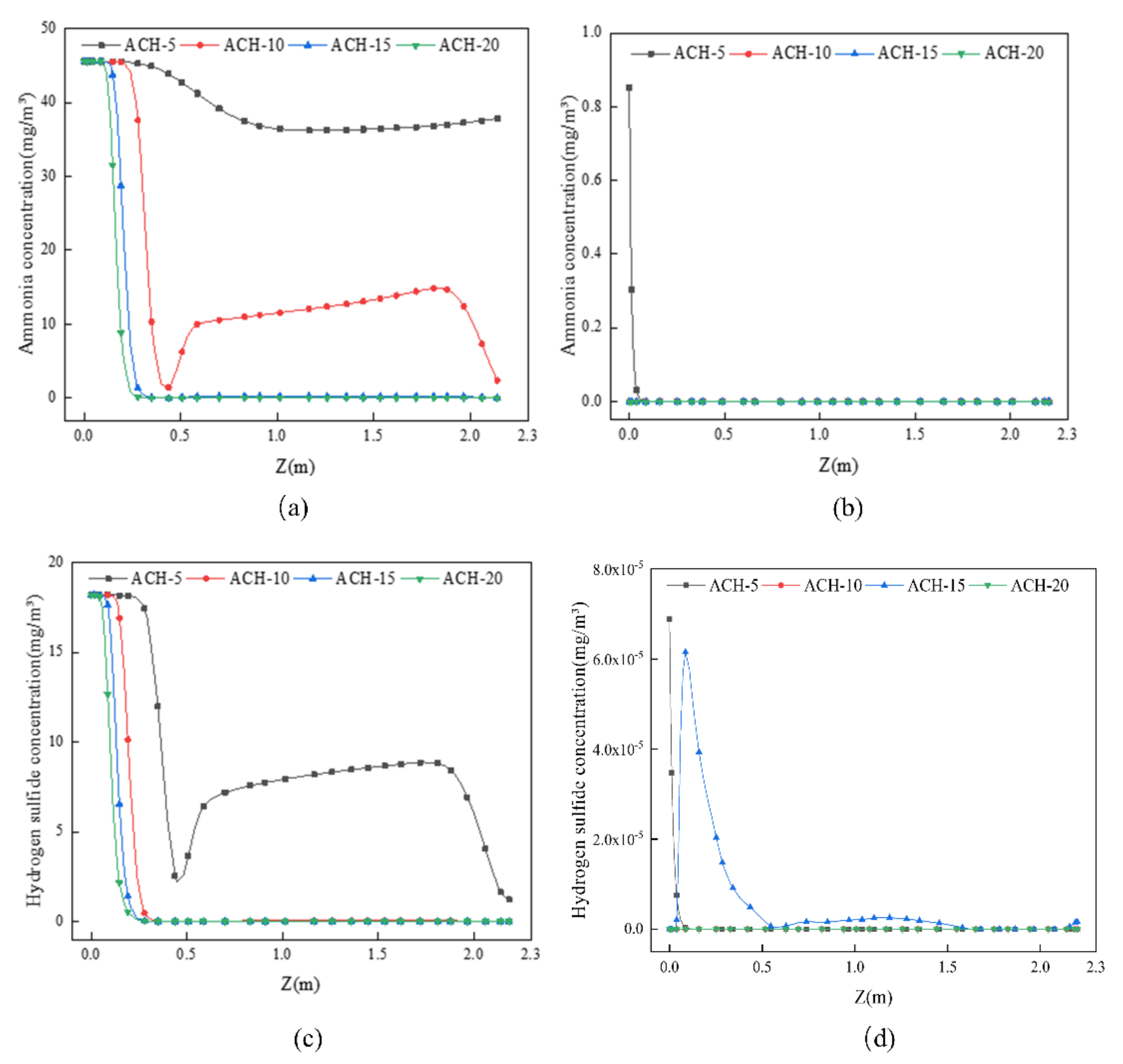
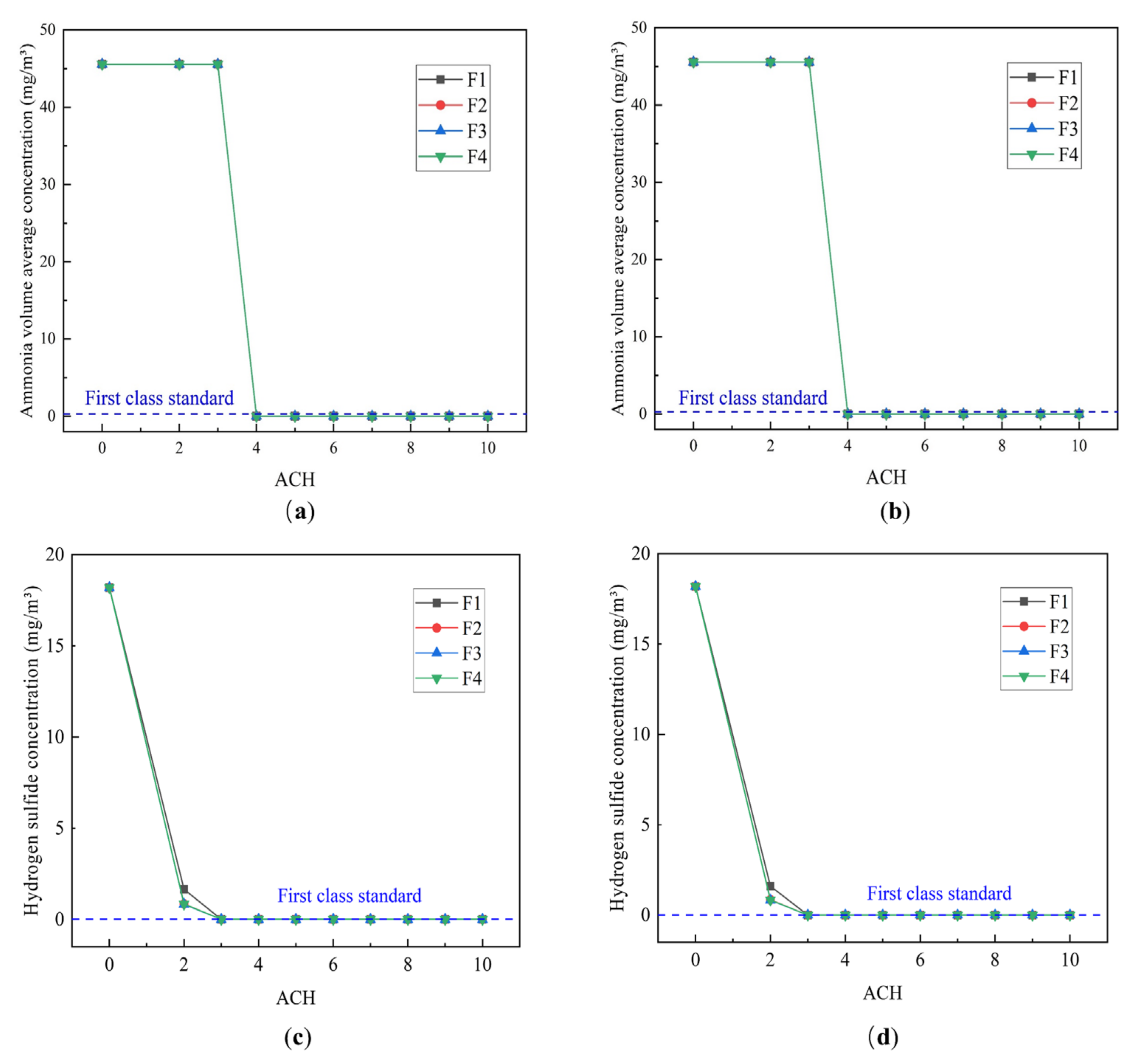
4.2.1. Effect of the ACH

Figure 11 shows the changes in contaminant concentration and removal efficiency as functions of the ACH for ammonia and hydrogen sulfide. At an ACH of 0 h−1 (i.e., the exhaust fan is turned off), the contaminant concentration is high. As the ACH increases, the VAC of hydrogen sulfide decreases (Figure 11c).
In contrast, in the case of ammonia, the VAC does not change between the ACH values of 0 h−1 and 3 h−1, although when the ACH exceeds 3 h−1, the VAC decreases rapidly. Furthermore, the ammonia concentration distribution results shown in Figure 12 indicate that the ammonia originates from the surface of the fermentation tank and diffuses through the toilet to the restroom. When the ACH is low, the ammonia is distributed uniformly in the space, as shown in Figure 12b. However, as the ACH increases, the contaminant concentrations in the space below decrease, and fewer contaminants spread to the top. As shown in Figure 13, the concentrations of hydrogen sulfide and ammonia gas exhibit similar trends in response to the ACH changes. At the same ACH, the concentration of hydrogen sulfide is lower than that of ammonia because hydrogen sulfide is denser than air, which restricts its upward diffusion.
The velocity contours in Figure 14 help illustrate the concentration distribution dynamics. When the ACH is 0 h−1, the ammonia gas diffuses upward freely, forming a vortex in the upper space, and it exists in the space for a longer time. Increasing the ACH to 2 h−1 results in a reduction in the upward emission rate of ammonia; however, the ammonia mixes fully with air. Therefore, the contaminant concentrations in the upper space are extremely high. When the ACH increases to 4 h−1, the air enters the toilet from the upper discharge port and is discharged together with the contaminants through the exhaust fan. Consequently, the airflow direction changes to inhibit the upward diffusion of ammonia. Therefore, the ammonia concentration in the upper part of the toilet is extremely low.
Compared with an exhaust without a fan, at an ACH of 4 h−1, the VAC of ammonia is reduced by 71.7% on average, with this reduction increasing to 85% and 88% on average at ACHs of 8 h−1 and 10 h−1, respectively. As in the case of ammonia, hydrogen sulfide diffuses upward freely and is distributed uniformly in the space at ACH = 0 h−1. At an ACH of 2 h−1, the hydrogen sulfide concentration in the upper space is extremely low, although this remains high in the lower space. However, increasing the ACH to 4 h−1 also results in a reduction in the hydrogen sulfide concentration in the lower space. Hydrogen sulfide and ammonia exhibit similar diffusion behaviors. When utilizing an exhaust without a fan, the VAC is reduced by 61.1%, 82%, 89.4%, and 89.8% on average for the ACH values of 2 h−1, 4 h−1, 8 h−1, and 10 h−1, respectively.
The concentrations of indoor pollutants in large spaces were explored by Duci et al. [53] using CFD modeling, with the results showing that reasonable mechanical ventilation can reduce the concentrations of indoor pollutants. Specifically, at the ventilation speeds of 1 m/s and 2 m/s, the pollutant concentrations in the local respiratory area of restroom users were reduced by 30% and 50%, respectively.
As shown in Figure S10, when the volume of air in the exhaust is relatively small, the pollutants diffuse into the upper space and are discharged from the grille and the upper air outlet. When the ACH exceeds a certain value, the grille and upper air outlet become air inlets, allowing fresh outdoor air to enter the room and improve the IAQ. As the ACH increases, an increasing amount of air enters the room, forming a vortex above the inlet and a significant sense of air blowing is felt by occupants. Therefore, the ACH should be maintained within a certain range to avoid causing discomfort to restroom users.
Figure 15 and Figure 16 show that the B-Z control level, that is, the average contaminant concentration in the B-Z, and VAC exhibit similar behaviors. For example, Figure 15 demonstrates that at an ACH of 4 h−1, a small amount of contaminant accumulates at the corners of the B-Z, whereas the average concentration approaches 0 mg × m−3. Moreover, Figure 16 indicates that an ACH exceeding 3 h−1 is sufficient to achieve a first-class standard regarding average contaminant concentration in the B-Z.
As the ACH increases, the CRE first increases, then decreases, and finally stabilizes, as shown in Figure 16. Hydrogen sulfide and ammonia removal efficiencies reach their peaks when the ACH is 3 h−1 and 4 h−1, respectively. The contaminant concentrations inside the toilet and the exhaust fan outlet gradually decrease with increasing ACH. These findings indicate that the ACH and CRE follow a nonlinear relationship in which the gain ratio is reduced when the ACH exceeds a certain value. Accordingly, the effect of the ACH can be divided into three stages. The first of these is the ‘ineffective exhaust’ stage, which is defined as the stage in which the contaminant cannot be removed, owing to an insufficient air supply velocity. At an ACH of 3 h−1, the concentration of ammonia gas is equal to that when there is no exhaust fan, and the ammonia gas is not fully discharged. Second, the ‘enhanced exhaust’ phase is defined as the stage in which the air supply velocity exceeds the critical velocity required to maintain a stable discharge of contaminants. Additional amounts of contaminants may be discharged by increasing the ACH, whereas the concentration of contaminants in the B-Z can be reduced to below the standard concentration required for an acceptable IAQ in restrooms.
Finally, ‘excessive ventilation’ is defined as the stage in which the average contaminant concentration in the B-Z inside the restroom does not decrease as the ACH increases because the concentration is close to 0 mg × m−3 and no longer changes. When the ACH is greater than 4 h−1, contaminant concentrations in the B-Z cease to change; therefore, increasing the volume of air in the exhaust has little effect on the contaminant discharge.

4.2.2. Effect of the Exhaust Fan Position

Figure 17a,b show that the ammonia gas concentration and CRE decrease and increase (nonlinearly), respectively, as the ACH increases. To some extent, the CRE is influenced by the EFP. When the ACH is between 3.1 h−1 and 3.3 h−1 and the exhaust fan is located at F1 or F2, the VAC is reduced, and CRE is maximized. A slight increase in the ACH to between 3.4 h−1 and 3.5 h−1 and relocating the exhaust fan to F3 also maximizes the CRE. At an ACH of 3.6 h−1, the concentrations of all contaminants are approximately equal. Furthermore, Figure 17c,d show that the contaminant concentrations in the B-Z change similarly with the ACH. When the ACH is less than 3.5 h−1, the substances in the exhaust do not satisfy the first-class standards. At an ACH of 3.5 h−1 and with the exhaust fan positioned at F3 rather than F4, the first-class standards may be achieved. By increasing the ACH slightly to 3.6 h−1, the first-class standards are satisfied for all the configurations examined in this study.
As shown in Figures S11 and S12, at an ACH of 3.3 h−1, there are differences in the distribution of pollutant concentrations in the upper part of the toilet. The closer the exhaust fan is to the pollution source, the shorter the time spent by the pollutant in the toilet and the lower the pollutant concentration in the toilet. When the exhaust fan is located at F1 or F2, fewer vortices are generated close to the pollution source, and the pollutants are discharged more easily. As shown in Figures S13 and S14, when the ACH is 3.6 h−1, the upper space of the toilet has very low pollutant concentrations. There is almost no difference between the restroom configurations. The pollutants exhibit minimal upward diffusion, with the majority of pollutants discharged through the exhaust fan. However, at lower pollutant concentrations, there is a certain difference: when the exhaust fan is positioned at F3 or F4, the high-concentration area is relatively large.
In summary, increasing the ACH causes the vortex in the upper space to grow, whereas part of the vortex is generated around the fermentation tank, which is not conducive to pollutant discharge. Figure S15a,b show that the average hydrogen sulfide concentration decreases with increasing ACH. Specifically, when the ACH increases from 2 h−1 to 2.1 h−1, the concentration of hydrogen sulfide decreases rapidly, whereas the ventilation efficiency increases rapidly. When the ACH is equal to at least 2.1 h−1 and the exhaust fan is in the F1 position, the pollutant concentration in the B-Z is at its lowest and the ventilation efficiency is at its highest. Conversely, relocating the exhaust fan to F4 results in the lowest observed ventilation efficiency. Figure S15c,d show that when the ACH is at least 2.2 h−1, the hydrogen sulfide concentration in the B-Z for each configuration meets the requirement for the first-class standard. Chung et al. [54] investigated the ventilation efficiencies of different ventilation configurations involving two inlet and two outlet diffusers at different locations. The results indicated that floor-based exhaust ventilation systems are effective in removing pollutant-related odors, with only 1.2% and 1.5% of pollutant particles remaining in the male and female restrooms, respectively.
Positioning the exhaust fan closer to the pollution source facilitates contaminant removal. However, as ammonia gas is less dense than air, it diffuses upward easily. In contrast, as hydrogen sulfide is denser than air, it accumulates below. The different spatial distributions of the ammonia and hydrogen sulfide arise from their different concentrations. The fermentation tank obstructs air circulation and changes the airflow direction, which causes vortices in some areas; consequently, the ventilation efficiency does not change linearly with increase in the ACH. In addition, the vortices mean that the optimal exhaust position depends on the ACH value. According to our rigorous analysis, an ACH of 3.5 h−1 provides the best solution overall. At this value, the average concentrations of ammonia and hydrogen sulfide satisfy the first-class standards, with the highest ventilation efficiency when the exhaust fan is placed at F4.

4.2.3. Effects of the Natural Vent Location

The positions of natural vents (L1, L2, L3, and L4) also influence the pollutant diffusion. To analyze this influence, the position of the exhaust fan was fixed at F4, and the VAC and CRE were calculated for ammonia and hydrogen sulfide, with the results shown in Figures S16 and S17. First, Figure S16 shows that when the ACH is between 3 h−1 and 3.6 h−1, the VAC is at its minimum (and the CRE is at the maximum) when the natural discharge port is located at L1. However, when the ACH exceeds 4 h−1, placing the natural discharge port at L3 yields the highest CRE. There is little variation in VAC between the various configurations. As shown in Figure S17, when the ACH is between 2 h−1 and 2.5 h−1, the VAC and CRE of each configuration are similar; however, when the ACH exceeds 3 h−1, positioning the natural discharge port at L3 results in the highest CRE and lowest VAC. When the exhaust fan discharge is low, the natural air intake in the upper part of the toilet has a low air volume and the airflow disturbance is less pronounced, reducing any negative effects on restroom user comfort.

5. Conclusions

CFD simulations were designed and performed to determine the CRE to investigate the effects and weights of various factors that influence the CRE and B-Z control level in orthogonal experiments on NFETs. Single-factor analysis was conducted based on the results obtained from the orthogonal tests. The main conclusions of this study are as follows:
  • Common toilet ventilation factors (e.g., the ACH) and factors specific to NFETs (e.g., the EFP, NVL, and G-h) were ranked based on their statistical significance as follows: EFP > ACH > NVL > G-h, with the EFP achieving statistical significance (p-value < 0.01) in the case of ammonia. The CRE is high when the exhaust fan is installed in the lower part of the toilet (near the fermentation tank).
  • Contaminant concentration distributions were simulated for different exhaust positions and air changes, with the results showing that both the ACH and exhaust fan location must be considered in toilet exhaust design. Toilet ventilation efficiency may be optimized by installing the exhaust at the optimal location, thus maximizing the air quality improvement inside the toilet.
  • The VAC decreases with increasing ACH, with the rate of decrease decelerating gradually. In contrast, the CRE first increases and then decreases before finally stabilizing in response to increasing ACH. The CRE varies between 1 and 3 but does not exceed 3, which may be related to the small size of the toilet investigated, and the relatively low pollutant concentrations contained within it.
  • Single-factor analysis revealed three stages of exhaust behavior, namely, “ineffective”, “enhanced”, and “excessive”. Beyond guaranteeing sufficient air quality, an appropriate number of air changes should be selected to reduce the energy consumption and indoor air speed, thus reducing the blowing sensation and improving user comfort.
The findings presented in this study provide a theoretical basis for the design of toilets with effective ventilation systems.

Supplementary Materials

The following are available online at https://www.mdpi.com/article/10.3390/en14227570/s1, Figure S1. Grid condition of CFD model and plane of observation. (a): CFD model; (b): Observation plane; (c): Grid condition of CFD model, Figure S2. Case descriptions. Case 1-F (0,0.62,0.59), Case 2-F (0.07,0.62,0.85); unit: m.(a) Case 1;(b) Case 2, Figure S3. Ammonia concentration at ABCD four-point vertical line in Case 1; ACH unit: h−1. (a): Point A (b): Point B; (c): Point C, (d): Point D, Figure S4. Ammonia concentration at ABCD four-point vertical line in Case 2; ACH unit: h−1. (a): Point A (b): Point B; (c): Point C, (d): Point D, Figure S5. Hydrogen sulfide concentration at the ABCD four-point vertical line in Case 1; ACH unit: h−1. (a): Point A (b): Point B; (c): Point C, (d): Point D, Figure S6. Hydrogen sulfide concentration at the ABCD four-point vertical line in Case 2; ACH unit: h−1. (a): Point A (b): Point B; (c): Point C, (d): Point D, Figure S7. Statistical significance analysis of the orthogonal experiment results regarding the VAC of ammonia, Figure S8. Statistical significance analysis of the orthogonal experiment results regarding the VAC of hydrogen sulfide, Figure S9. Statistical significance analysis of the orthogonal experiment results regarding the CRE of hydrogen sulfide, Figure S10. Velocity vector contours for different ACH (unit: h−1) values. (a): ACH = 0; (b): ACH = 2; (c): ACH = 4; (d): ACH = 6; (e): ACH = 8; (f): ACH = 10, Figure S11. Ammonia concentration distributions for different positions of the exhaust fan (ACH = 3.3 h−1). (a): F1, (b): F2; (c): F3, (d): F4, Figure S12. Ammonia diffusion dynamics for different positions of the exhaust fan (ACH = 3.3 h−1). (a): F1, (b): F2; (c): F3, (d): F4, Figure S13. Ammonia concentration distributions for different positions of the exhaust fan (ACH = 3.6 h−1). (a): F1, (b): F2; (c): F3, (d): F4, Figure S14. Ammonia diffusion dynamics for different positions of the exhaust fan (ACH = 3.6 h−1). (a): F1, (b): F2; (c): F3, (d): F4, Figure S15. Average concentration and CRE of (a,b) hydrogen sulfide and (c,d) hydrogen sulfide in the breathing zone for different ACH values. VAC: volume average concentration; CRE: contaminant removal efficiency; ACH unit: h−1. (a): VAC, (b): CRE; (c): Z = 0.9 m, (d): Z = 1.5 m, Figure S16. (a,c) Average volume concentration and (b,d) CRE of ammonia in the breathing zone for different ACH (unit: h−1) values. (a): VAC(ACH = 3.1–3.6), (b): CRE(ACH = 3.1–3.6); (c): VAC(ACH = 4–10), (d): CRE(ACH = 4–10), Figure S17. (a,c) Average volume concentration and (b,d) CRE of hydrogen sulfide in the breathing zone for different ACH (unit: h−1) values. (a): VAC(ACH = 2–2.5), (b): CRE(ACH = 2–2.5); (c): VAC(ACH = 3–10), (d): CRE(ACH = 3–10), Table S1. Summary of the experiments proposed according to the orthogonal design approach.

Author Contributions

Conceptualization, Z.Z. and X.Z.; methodology, Z.Z. and L.Z.; software, Z.Z. and L.Z.; validation, Z.Z., H.S. and Z.Y.; formal analysis, Z.Z. and W.Y.; investigation, Z.Z. and G.Y.; resources, J.G., L.W. and Y.Z.; data curation, Z.Z. and W.Y.; writing—original draft preparation, Z.Z.; writing—review and editing, Z.Z.; visualization, Z.Z.; supervision, X.Z.; project administration, X.Z.; funding acquisition, X.Z. All authors have read and agreed to the published version of the manuscript.

Funding

This research was funded by the National Key R&D Program of China grant number 2020YFD1100102-1.

Conflicts of Interest

The authors declare no conflict of interest.

Abbreviations

CAverage concentration of contaminants in the immediate environment (mg × m−3)
CeConcentration of contaminants at the exhaust outlet (mg × m−3)
CinConcentration of contaminants at the air supply outlet (mg × m−3)
IAQIndoor air quality
CREContaminant removal efficiency
NFETNon-flushing ecological toilet
CFDComputational fluid dynamics
EFPExhaust fan position
ACHAir change rate per hour (h−1)
NVLNatural vent location
G-hGrid height (m)

References

  1. Cheng, S.K.; Li, Z.F.; Uddin, S.M.N.; Mang, H.P.; Zhou, X.Q.; Zhang, J.; Zheng, L.L.; Zhang, L.L. Toilet revolution in China. J. Environ. Manag. 2018, 216, 347–356. [Google Scholar] [CrossRef]
  2. Sato, H.; Hirose, T.; Kimura, T.; Moriyama, Y.; Nakashima, Y. Analysis of Malodorous Volatile Substances of Human Waste: Feces and Urine. J. Health Sci. 2001, 47, 483–490. [Google Scholar] [CrossRef] [Green Version]
  3. Zhang, F.D.; Zhang, S.Q.; Wang, U.J.; Dou, F.G.; Xiu-Mei, L.I.; Zou, S.W. Deodorization Techniques on Fleeting Continuous Zymosis of Organic Feces with High Temperature. J. Agro. Environ. Sci. 2004, 23, 796a800. [Google Scholar]
  4. Kikuchi, R. Pilot-scale test of a soil filter for treatment of malodorous gas. Soil Use Manag. 2006, 16, 211–214. [Google Scholar] [CrossRef]
  5. Lewkowska, P.; Cieślik, B.; Dymerski, T.; Konieczka, P.; Namieśnik, J. Characteristics of odors emitted from municipal wastewater treatment plant and methods for their identification and deodorization techniques. Environ. Res. 2016, 151, 573–586. [Google Scholar] [CrossRef]
  6. Kanjanarong, J.; Giri, B.S.; Jaisi, D.P.; de Oliveira, F.R.; Boonsawang, P.; Chaiprapat, S.; Singh, R.; Balakrishna, A.; Khanal, S.K. Removal of hydrogen sulfide generated during anaerobic treatment of sulfate-laden wastewater using biochar: Evaluation of efficiency and mechanisms. Bioresour. Technol. 2017, 234, 115–121. [Google Scholar] [CrossRef]
  7. Yamamoto, T.; Uchida, M.; Kurihara, Y. Deodorant compositions containing antibacterial zeolite and silicones. Zeolites 1997, 18, 235. [Google Scholar] [CrossRef]
  8. Wang, J.; Xiao, Y.; Tao, J.; Liang, H.; Wu, Z. An Introduction of Automatic Catalytic Oxidation Active Carbon Odor Control Technology. Guangdong Chem. Ind. 2008, 20, 141–144. [Google Scholar]
  9. Osako, M.; Nishida, K. Mechanisms of the sensory deodorization by aromatic deodorizers. Counteraction and masking effect of aromatic compounds. Jpn. J. Ergon. 1990, 26, 271–282. [Google Scholar] [CrossRef] [Green Version]
  10. Fang, L.; Norris, C.; Johnson, K.; Cui, X.; Sun, J.; Teng, Y.; Tian, E.; Xu, W.; Li, Z.; Mo, J.; et al. Toxic volatile organic compounds in 20 homes in Shanghai: Concentrations, inhalation health risks, and the impacts of household air cleaning. Build. Environ. 2019, 157, 309–318. [Google Scholar] [CrossRef]
  11. Ao, Y.; Wang, L.; Jia, X.; Gu, C. Numerical Simulation of Pollutant Diffusion Law in Bathroom and Optimization of the Locations and Ways of Exhaust Outlet and Makeup Air, Shenyang Jianzhu Daxue Xuebao (Ziran Kexue Ban). J. Shenyang Jianzhu Univ. 2011, 27, 720–724. [Google Scholar]
  12. Han, Z.; Xu, Y.; Wang, H.; Tian, H.; Qiu, B.; Sun, D. Synthesis of ammonia molecularly imprinted adsorbents and ammonia adsorption separation during sludge aerobic composting. Bioresour. Technol. 2019, 300, 122670. [Google Scholar] [CrossRef] [PubMed]
  13. Zhang, D.; Liu, J.; Liu, L. On the capture of polar indoor air pollutants at sub-ppm level—A molecular simulation study. Build. Simul. 2020, 13, 989–997. [Google Scholar] [CrossRef]
  14. Vikrant, K.; Kailasa, S.K.; Tsang, D.; Lee, S.S.; Kumar, P.; Giri, B.S.; Singh, R.S.; Kim, K.-H. Biofiltration of hydrogen sulfide: Trends and challenges. J. Clean. Prod. 2018, 187, 131–147. [Google Scholar] [CrossRef]
  15. Tian, K.; Wang, X.X.; Yu, Z.Y.; Li, H.; Xin, G. Hierarchical and hollow Fe2O3 nano-boxes derived from metal-organic frameworks with excellent sensitivity to H2S. Acs Appl. Mater. Interfaces 2017, 9. [Google Scholar] [CrossRef] [PubMed]
  16. Yang, G.; Wu, L. Trend in H2S Biology and Medicine Research—A Bibliometric Analysis. Molecules 2017, 22, 2087. [Google Scholar] [CrossRef] [Green Version]
  17. Wei, Y.; Xu, Z.; Gao, J.; Cao, G.; Xiang, Z.; Xing, S. Indoor air pollutants, ventilation rate determinants and potential control strategies in Chinese dwellings: A literature review. Sci. Total Environ. 2017, 586, 696–729. [Google Scholar]
  18. Kato, S.; Yang, J.-H. Study on inhaled air quality in a personal air-conditioning environment using new scales of ventilation efficiency. Build. Environ. 2008, 43, 494–507. [Google Scholar] [CrossRef]
  19. Novoselac, A.; Srebric, J. Comparison of Air Exchange Efficiency and Contaminant Removal Effectiveness as IAQ Indices. ASHRAE Trans. 2003, 109, 339–349. [Google Scholar]
  20. Laverge, J.; Spilak, M.; Novoselac, A. Experimental assessment of the inhalation zone of standing, sitting and sleeping persons. Build. Environ. 2014, 82, 258–266. [Google Scholar] [CrossRef]
  21. Sandberg, M.; Blomqvist, C. Displacement ventilation systems in office rooms. ASHRAE Trans. 1989, 95, 1041–1049. [Google Scholar]
  22. American Society of Heating. Refrigerating and air-conditioning engineers. Int. J. Refrig. 1979, 2, 56–57. [Google Scholar] [CrossRef] [Green Version]
  23. Lin, Y.-P. Natural Ventilation of Toilet Units in K–12 School Restrooms Using CFD. Energies 2021, 14, 4792. [Google Scholar] [CrossRef]
  24. Ponechal, R.; Krušinský, P.; Kysela, P.; Pisca, P. Simulations of Airflow in the Roof Space of a Gothic Sanctuary Using CFD Models. Energies 2021, 14, 3694. [Google Scholar] [CrossRef]
  25. Khosravi, S.N.; Mahdavi, A. A CFD-Based Parametric Thermal Performance Analysis of Supply Air Ventilated Windows. Energies 2021, 14, 2420. [Google Scholar] [CrossRef]
  26. Seduikyte, L.; Stasiulienė, L.; Prasauskas, T.; Martuzevičius, D.; Černeckienė, J.; Ždankus, T.; Dobravalskis, M.; Fokaides, P. Field Measurements and Numerical Simulation for the Definition of the Thermal Stratification and Ventilation Performance in a Mechanically Ventilated Sports Hall. Energies 2019, 12, 2243. [Google Scholar] [CrossRef] [Green Version]
  27. Yang, G.; Li, X.; Ding, L.; Zhu, F.; Wang, Z.; Wang, S.; Xu, Z.; Xu, J.; Qiu, P.; Guo, Z. CFD Simulation of Pollutant Emission in a Natural Draft Dry Cooling Tower with Flue Gas Injection: Comparison between LES and RANS. Energies 2019, 12, 3630. [Google Scholar] [CrossRef] [Green Version]
  28. Chung, S.-C.; Lin, Y.-P.; Yang, C.; Lai, C.-M. Natural Ventilation Effectiveness of Awning Windows in Restrooms in K-12 Public Schools. Energies 2019, 12, 2414. [Google Scholar] [CrossRef] [Green Version]
  29. Conceio, E.; Awbi, H. Evaluation of Integral Effect of Thermal Comfort, Air Quality and Draught Risk for Desks Equipped with Personalized Ventilation Systems. Energies 2021, 14, 3235. [Google Scholar] [CrossRef]
  30. Cho, J. Investigation on the contaminant distribution with improved ventilation system in hospital isolation rooms: Effect of supply and exhaust air diffuser configurations. Appl. Therm. Eng. 2018, 148, 208–218. [Google Scholar] [CrossRef]
  31. Tung, Y.-C.; Hu, S.-C.; Tsai, T.-Y. Influence of bathroom ventilation rates and toilet location on odor removal. Build. Environ. 2009, 44, 1810–1817. [Google Scholar] [CrossRef]
  32. Tung, Y.-C.; Hu, S.-C.; Tsai, T.-I.; Chang, I.-L. An experimental study on ventilation efficiency of isolation room. Build. Environ. 2009, 44, 271–279. [Google Scholar] [CrossRef]
  33. Tung, Y.-C.; Shih, Y.-C.; Hu, S.-C.; Chang, Y.-L. Experimental performance investigation of ventilation schemes in a private bathroom. Build. Environ. 2010, 45, 243–251. [Google Scholar] [CrossRef]
  34. Quitzau, M.B. Water-flushing toilets: Systemic development and path-dependent characteristics and their bearing on techno-logical alternatives. Technol. Soc. 2007, 29, 351–360. [Google Scholar] [CrossRef]
  35. Sutherland, C.; Reynaert, E.; Dhlamini, S.; Magwaza, F.; Lienert, J.; Riechmann, M.E.; Buthelezi, S.; Khumalo, D.; Morgenroth, E.; Udert, K.M.; et al. Socio-technical analysis of a sanitation innovation in a peri-urban household in Durban, South Africa. Sci. Total. Environ. 2020, 755, 143284. [Google Scholar] [CrossRef]
  36. Tada, S.; Itoh, Y.; Kiyoshi, K.; Yoshida, N. Isolation of ammonia gas-tolerant extremophilic bacteria and their application to the elimination of malodorous gas emitted from outdoor heat-treated toilets. J. Biosci. Bioeng. 2021, 131, 509–517. [Google Scholar] [CrossRef]
  37. Bhagwan, J.N.; Pillay, S.; Koné, D. Sanitation game changing: Paradigm shift from end-of-pipe to off-grid solutions. Water Pract. Technol. 2019, 14, 497–506. [Google Scholar] [CrossRef]
  38. Anand, C.K.; Apul, D.S. Composting toilets as a sustainable alternative to urban sanitation—A review. Waste Manag. 2014, 34, 329–343. [Google Scholar] [CrossRef]
  39. Nielsen, P.V. Fifty years of CFD for room air distribution. Build. Environ. 2015, 91, 78–90. [Google Scholar] [CrossRef]
  40. Rong, L.; Nielsen, P.V.; Bjerg, B.; Zhang, G. Summary of best guidelines and validation of CFD modeling in livestock buildings to ensure prediction quality. Comput. Electron. Agric. 2016, 121, 180–190. [Google Scholar] [CrossRef]
  41. Shen, C.; Gao, N.; Wang, T. CFD study on the transmission of indoor pollutants under personalized ventilation. Build. Environ. 2013, 63, 69–78. [Google Scholar] [CrossRef]
  42. Lv, L.; Gao, J.; Zeng, L.; Cao, C.; Zhang, J.; He, L. Performance assessment of air curtain range hood using contaminant removal efficiency: An experimental and numerical study. Build. Environ. 2020, 188, 107456. [Google Scholar] [CrossRef]
  43. Lv, L.; Zeng, L.; Wu, Y.; Gao, J.; Xie, W.; Cao, C.; Chen, Y.; Zhang, J. Effects of human walking on the capture efficiency of range hood in residential kitchen. Build. Environ. 2021, 196, 107821. [Google Scholar] [CrossRef]
  44. Zeng, L.; Liu, G.; Gao, J.; Du, B.; Lv, L.; Cao, C.; Ye, W.; Tong, L.; Wang, Y. A circulating ventilation system to concentrate pollutants and reduce exhaust volumes: Case studies with experiments and numerical simulation for the rubber refining process. J. Build. Eng. 2020, 35, 101984. [Google Scholar] [CrossRef]
  45. Yong, Z.A.; Xia, Y.A.; Hy, A.; Kz, A.; Xw, B.; Zl, C.; Jian, H.; Sz, A. Numerical investigations of reactive pollutant dispersion and personal exposure in 3D urban-like models. Build. Environ. 2019, 169, 106569. [Google Scholar]
  46. Yang, X.; Yang, H.; Ou, C.; Luo, Z.; Hang, J. Airborne transmission of pathogen-laden expiratory droplets in open outdoor space. Sci. Total. Environ. 2021, 773, 145537. [Google Scholar] [CrossRef]
  47. Tong, L.; Gao, J.; Luo, Z.; Wu, L.; Zeng, L.; Liu, G.; Wang, Y. A novel flow-guide device for uniform exhaust in a central air exhaust ventilation system. Build. Environ. 2019, 149, 134–145. [Google Scholar] [CrossRef]
  48. Shaojie, J.; Jinfeng, M. Pollutant Concentration Research of Toilet in Natural Ventilation Conditions. Contam. Control. Air-Cond. Technol. 2012, 4. [Google Scholar]
  49. The Standardization Administration of the People’s Republic of China, Hygienic Standards for Communal Toilet in City, Domestic-National Standards-State Administration for Market Regulation CN-GB. 1998. Available online: https://max.book118.com/html/2019/0429/8125027036002021.shtm (accessed on 15 August 2021).
  50. Wu, W.Z. Yuanfang, Urban public toilet design standards, Domestic-Industry Standard-Industry Standard-Urban Construction CN-CJ, China Construction Industry Press. 2016. Available online: http://www.mohurd.gov.cn/wjfb/201703/t20170306_230861.html (accessed on 15 August 2021).
  51. Lu, Y. HVAC Design Guidelines; China Construction Industry Press: Beijing, China, 1996. [Google Scholar]
  52. Liu, W.; Liu, D.; Gao, N. CFD study on gaseous pollutant transmission characteristics under different ventilation strategies in a typical chemical laboratory. Build. Environ. 2017, 126, 238–251. [Google Scholar] [CrossRef]
  53. Duci, A.; Papakonstantinou, K.; Chaloulakou, A.; Markatos, N. Numerical approach of carbon monoxide concentration dis-persion in an enclosed garage. Build. Environ. 2004, 39, 1043–1048. [Google Scholar] [CrossRef]
  54. Chung, K.-C.; Hsu, S.-P. Effect of ventilation pattern on room air and contaminant distribution. Build. Environ. 2001, 36, 989–998. [Google Scholar] [CrossRef]
Figure 1. Research model geometry, gas detector, and monitoring points: P1 (0.48, 0.48, 0.9), P2 (0.48, 0.48, 1), P3 (0.48, 0.48, 1.2), P4 (0.48, 0.48, 1.4), P5 (0.48, 0.48, 1.9); unit: m. 1—Grid, 2—Pollution source, 3—Window (a) Model diagram; (b) Test bench; (c) Front view; (d) XLA-BX-SF6 gas detector; (e) PNT400-H2S/O3/NH3-G gas detector.
Energies 14 07570 g001
Figure 2. SF6 and ammonia concentrations at different locations. (a) Grid independence verification (test bench). (b) Validation of the SF6 concentration at different locations. (c) Grid independence verification (restroom model).
Energies 14 07570 g002
Figure 3. Schematic of the experimental chamber and location of sampling points. Points F1 (0,0.13,0.59), F2 (0,0.62,0.59), F3 (0,1.11,0.59), F4 (0,1.11,0.1), F5 (0.07,0.62,0.85), unit: m. 1—Grid, 2—Fan, 3—Window, 4—Pollution source, 5—Fermentation tank, (a) Model diagram; (b) Front view; (c) Top view.
Energies 14 07570 g003
Figure 4. Contaminant concentrations along the vertical line at point E for different cases. Ammonia: (a): Case 1; (b): Case 2; Hydrogen sulfide: (c): Case 1; (d): Case 2.
Energies 14 07570 g004
Figure 5. Ammonia concentration distributions with different ACH (unit: h−1) values for Cases 1 and 2. Case 1: (a) ACH = 5, (b) ACH = 10; Case 2: (c) ACH = 5, (d) ACH = 10.
Energies 14 07570 g005
Figure 6. Hydrogen sulfide concentration distributions at different ACH (unit: h−1) values for Cases 1 and 2. Case 1: (a) ACH = 5, (b) ACH = 10; Case 2: (c) ACH = 5, (d) ACH = 10.
Energies 14 07570 g006
Figure 7. Streamline contours under different ACH (unit: h−1) values for Cases 1 and 2. Case 1: (a) ACH = 5, (b) ACH = 10; Case 2: (c) ACH = 5, (d) ACH = 10.
Energies 14 07570 g007
Figure 8. Contours of air age under different ACH (unit: h−1) values for Cases 1 and 2. Case 1: (a) ACH = 5, (b) ACH = 10; Case 2: (c) ACH = 5, (d) ACH = 10.
Energies 14 07570 g008
Figure 9. Statistical analysis of ammonia and hydrogen sulfide removal. Ammonia: (a): VAC; (b): CRE; Hydrogen sulfide: (c): VAC; (d): CRE.
Energies 14 07570 g009
Figure 10. Statistical significance analysis of the orthogonal experiment results for the CRE of ammonia.
Energies 14 07570 g010
Figure 11. Changes in VAC and CRE as functions of the ACH (unit: h−1) for ammonia and hydrogen sulfide. Ammonia: (a): VAC; (b): CRE; Hydrogen sulfide: (c): VAC; (d): CRE.
Energies 14 07570 g011
Figure 12. Ammonia concentration distributions for different ACH (unit: h−1) values (EFP-F1). (a): ACH = 0; (b): ACH = 2; (c): ACH = 4; (d): ACH = 6; (e): ACH = 8; (f): ACH = 10.
Energies 14 07570 g012
Figure 13. Hydrogen sulfide concentration distributions for different ACH (unit: h−1) values (EFP-F1). (a): ACH = 0; (b): ACH = 2; (c): ACH = 4; (d): ACH = 6; (e): ACH = 8; (f): ACH = 10.
Energies 14 07570 g013
Figure 14. Ammonia diffusion dynamics for different ACH (unit: h−1) values (EFP-F1). (a): ACH = 0; (b): ACH = 2; (c): ACH = 4; (d): ACH = 6; (e): ACH = 8; (f): ACH = 10.
Energies 14 07570 g014
Figure 15. Ammonia concentration distributions for different ACH (unit: h−1) values (Z = 0.9 m EFP-F1). (a): ACH = 0; (b): ACH = 2; (c): ACH = 4; (d): ACH = 6; (e): ACH = 8; (f): ACH = 10.
Energies 14 07570 g015
Figure 16. Average concentrations of (a,b) ammonia and (c,d) hydrogen sulfide in the B-Z for different ACH (unit: h−1) values. (a): Z = 0.9 m, (b): Z = 1.5 m; (c): Z = 0.9 m, (d): Z = 1.5 m.
Energies 14 07570 g016
Figure 17. (a,c) Average volume concentration and (b,d) CRE of ammonia in the B-Z for different ACH (unit: h−1) values. (a): VAC, (b): CRE; (c): Z = 0.9 m, (d): Z = 1.5 m.
Energies 14 07570 g017
Table 1. Concentration standards for ammonia and hydrogen sulfide in public toilets.
ContaminantsFirst Class StandardSecond Class StandardThird Class Standard
Ammonia (mg/m³)0.313
Hydrogen sulfide (mg/m³)0.010.010.01
Publisher’s Note: MDPI stays neutral with regard to jurisdictional claims in published maps and institutional affiliations.

