Abstract
This paper applies a voltage instability monitoring method based on voltage and current measurements from a transmission bus PMU on the Hellenic Interconnected System using both unstable and marginally stable scenarios, derived from the historical 12 July 2004 blackout of the Athens area. The effectiveness, selectivity and reliability of the proposed monitoring method is clearly demonstrated, allowing its integration into a System Protection Scheme with direct load shedding. It is shown that the proposed instability detection and control scheme could have prevented the voltage collapse if applied at the time of the event.
1. Introduction
Voltage stability has been a well established area of power system research for several decades, and its theoretical aspects, underlying phenomena as well as mechanisms of instability, have been well described in the literature [1,2]. Nonetheless, transmission systems may still face stressed and insecure operating conditions, which could threaten stability. The transition of power systems due to the market deregulation and renewable integration has resulted in power systems operating under dispatch schemes and power flow patterns, for which the systems had not been initially planned. This reality brings voltage stability analysis and system protection schemes against voltage collapse once again to the forefront.
On-line voltage instability detection systems are key components for the protection of power systems against extreme disturbances, and may be combined with response based System Protection Schemes (SPS) [3] for timely activating corrective actions, when voltage instability is identified without having to rely on operator response. Various centralized as well as decentralized identification methods have been proposed in the literature [4,5,6,7]. Recent developments focus on schemes that take advantage of the distributed generation, using the concept of active distribution networks [8,9], while other approaches rely on neural networks for classifying system disturbances and relating them with proper countermeasures based on the system dynamics [10].
Wide area monitoring and protection are gradually gaining ground, mainly due to the growing development and installation of PMUs that provide input to wide-area monitoring systems (WAMS). One of the most favorable attributes of WAMS constitute their capabilities to provide timely protection against instability, voltage instability being one of the applications. While several approaches for wide-area voltage stability identification and protection have been proposed in the literature, such as [11,12,13,14,15], few reports of actual industrial applications for wide area protection schemes against voltage instability, such as [16], have been published so far.
In this paper, a simple, and easy to apply in real life, wide-area system protection (WAP) system is presented. The protection system is based on phasor measurements and combines long-term voltage instability detection with direct load shedding, in order to protect against voltage instability and collapse. A main advantage of the presented WAP system lies in the fact that it is activated based on voltage instability detection conditions and not on any predefined voltage thresholds. This is an important factor providing selectivity to the protection scheme considering the constantly changing network conditions.
The voltage instability detection is based on the New LIVES index (NLI), originally presented in [17], as well as on the Relay-based Index (RLI) presented in [18]. Several load shedding schemes can be combined with this particular instability monitoring scheme. In the current paper the Hellenic Interconnected System (HIS) is simulated in the historical condition of 12 July 2004, which led to the Athens blackout [19]. The simulated incident is then used to demonstrate the operation of the proposed voltage instability detection method, followed by the activation of the load shedding scheme in the area of Athens available at that time. Further information on load-shedding schemes can be found in [20,21].
The structure of the paper is as follows: in Section 2, the NLI and RLI methods are summarized and the voltage instability detection system is described. Section 3 includes a brief description of the HIS and the utilization of the detection system in this case, as well as the derived stable and unstable scenarios used in this paper. Section 4 includes simulation results of the proposed detection instability system while its incorporation into an SPS with direct load shedding is presented in Section 5. Finally, in Section 6 the conclusions of the paper are summarized.
2. Transmission Bus Indices and Instability Detection System
NLI was originally presented in [17], where it was illustrated by means of full-time scale, as well as Quasi Steady-State (QSS) simulations on the IEEE Nordic Test System. Long-term voltage instability of a weak system area can be timely identified with NLI, when phasor measurements are available at the boundary buses of the weak area.
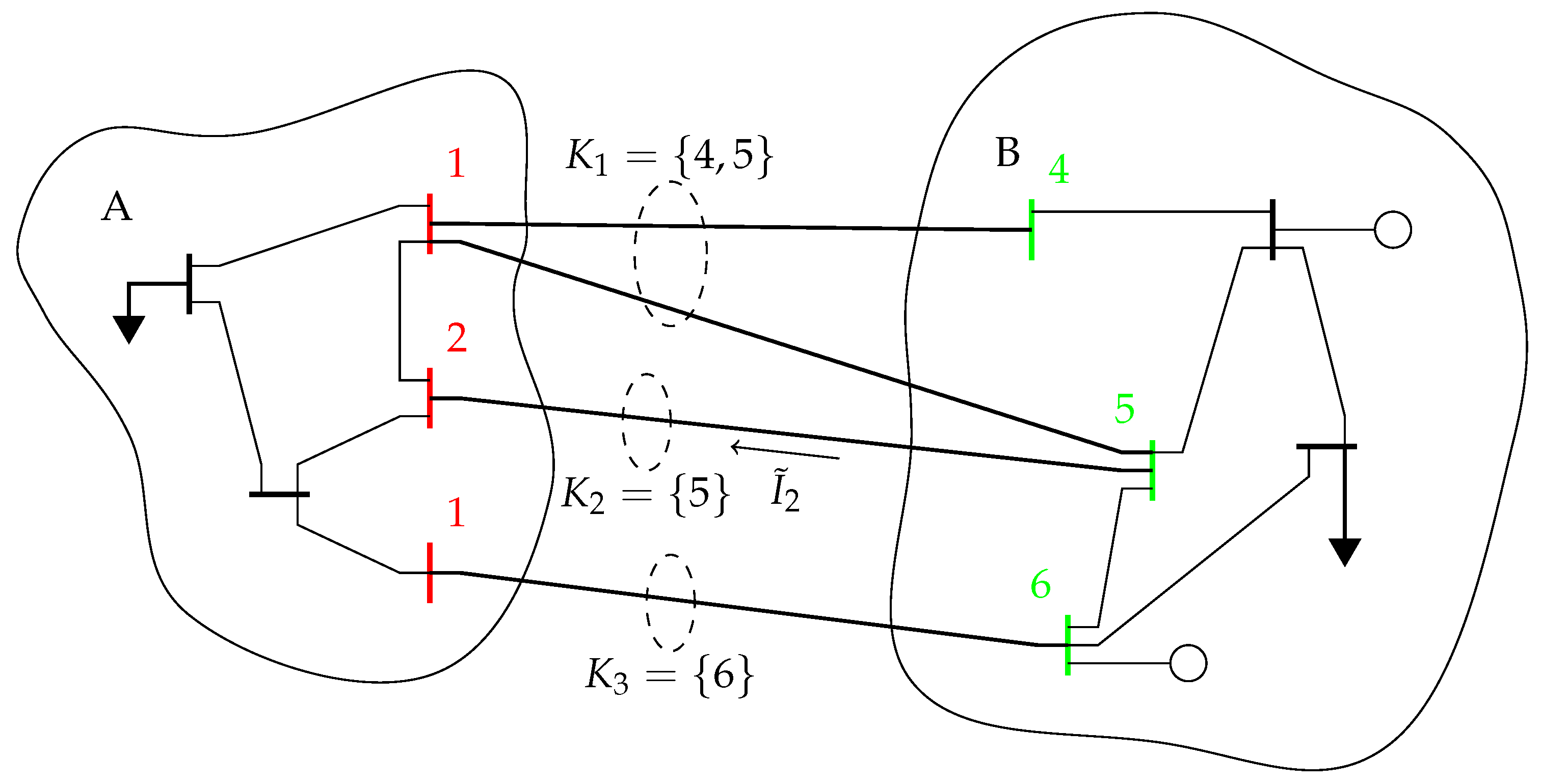
More specifically, this voltage instability identification method continuously records bus voltage and line current measurements, thereby forming two derived quantities, namely the bus receiving active power, as well as the apparent conductance as seen by the bus where the measurements are taken. It is noted that only the currents of the lines belonging to a particular cut-set (Figure 1) are needed. The NLI index is computed at the i-th boundary bus according to the following formula:
where signifies the change between two time instances, is the receiving active power at the i-th boundary bus, that is, the power flow through the transmission lines belonging to the cut-set, while corresponds to the apparent conductance, as seen at the particular boundary bus considering the receiving current , which can be calculated as follows:
where is the set containing the indices (j) of the corridor sending-end buses connected to bus i, as shown in Figure 1.
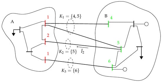
Figure 1.
Power transmission corridor with cut-set between receiving area A and sending area B. Receiving boundary buses in red, sending boundary buses in green.
Thus the received active power and apparent conductance can be calculated using the following equations:
where is the voltage phasor of bus i.
As has been discussed in [17], the calculated active power and apparent conductance can be efficiently filtered by means of the short-term Fourier transform, in order to suppress fast system dynamics, which fall outside the scope of long-term voltage stability monitoring, such as power oscillations, as well as measurement noise. However, in the current paper, the analysis is restricted to QSS simulations, implying that at each time instant the system operating point (and therefore each current and voltage measurement) is a short-term equilibrium. This means that the instantaneous NLI value corresponds to the operating point at which all fast dynamics have died out (see Section 4.1), thereby not necessitating any additional filtering apart from an averaging procedure, which accounts for the last N number of measurements. In the current article, N is set equal to 10. For the 1 time step used in the simulation this leads to a 10 s averaging period, which is sufficient to filter out transients and at the same time is representative of the actual filtering delay in a real system.
In addition, in order to account for large system disturbances such as short-circuits, line or other large outages, the NLI is calculated only when per time step falls within a reasonable band, that is:
Also, NLI is calculated only when apparent conductance difference per time step is positive (load increase) and it exceeds a minimum value, so as to avoid changes due to measurement noise, that is:
Positive NLI values signify stable system response to a demand increase of the monitored area, that is, the system is able to increase the transmitted active power through the transmission corridor. Once the system cannot meet the monitored area increasing demand, the transmitted active power reaches a maximum, while G continues to increase. This inability of the system to restore the demand is identified through an index sign change from positive to negative. As has been discussed in [17], this identification tends to occur quite close to the actual system instability onset.
In addition to NLI, which is based on PMUs at specific boundary buses, an alternative metric for long-term voltage instability identification has been presented in [18]. This method is based on a protective relay function that takes advantage of the numerical capabilities of modern microprocessor-based transmission line protective relays by sampling analogue voltage and current in the same manner as the NLI does and calculates in real-time the Local Relay-based Index (RLI) for local voltage instability identification and alarm. The RLI may be calculated either at the sending boundary buses or at the receiving ones. The calculation of the RLI proceeds very similarly with the ones of NLI, namely:
where and correspond to the transmitted active power of the transmission line connecting buses i and j and the apparent conductance as seen by the relay at bus i looking into the line. In case of calculating the RLI at the receiving boundary bus, the current polarity is reversed.
As has been shown in [18], RLI can also timely identify an imminent voltage instability despite its limited information in comparison to NLI. The idea of monitoring several boundary buses or digital relays surrounding an area prone to long-term voltage instability, constitutes a real-time wide-area monitoring system against long-term voltage instability.
The alarm signal, when issued either by the NLI or RLI may be sent to the control centre to be used as part (trigger) of an SPS.
3. Application of NLI and RLI in the Hellenic System of 2004
3.1. System Description
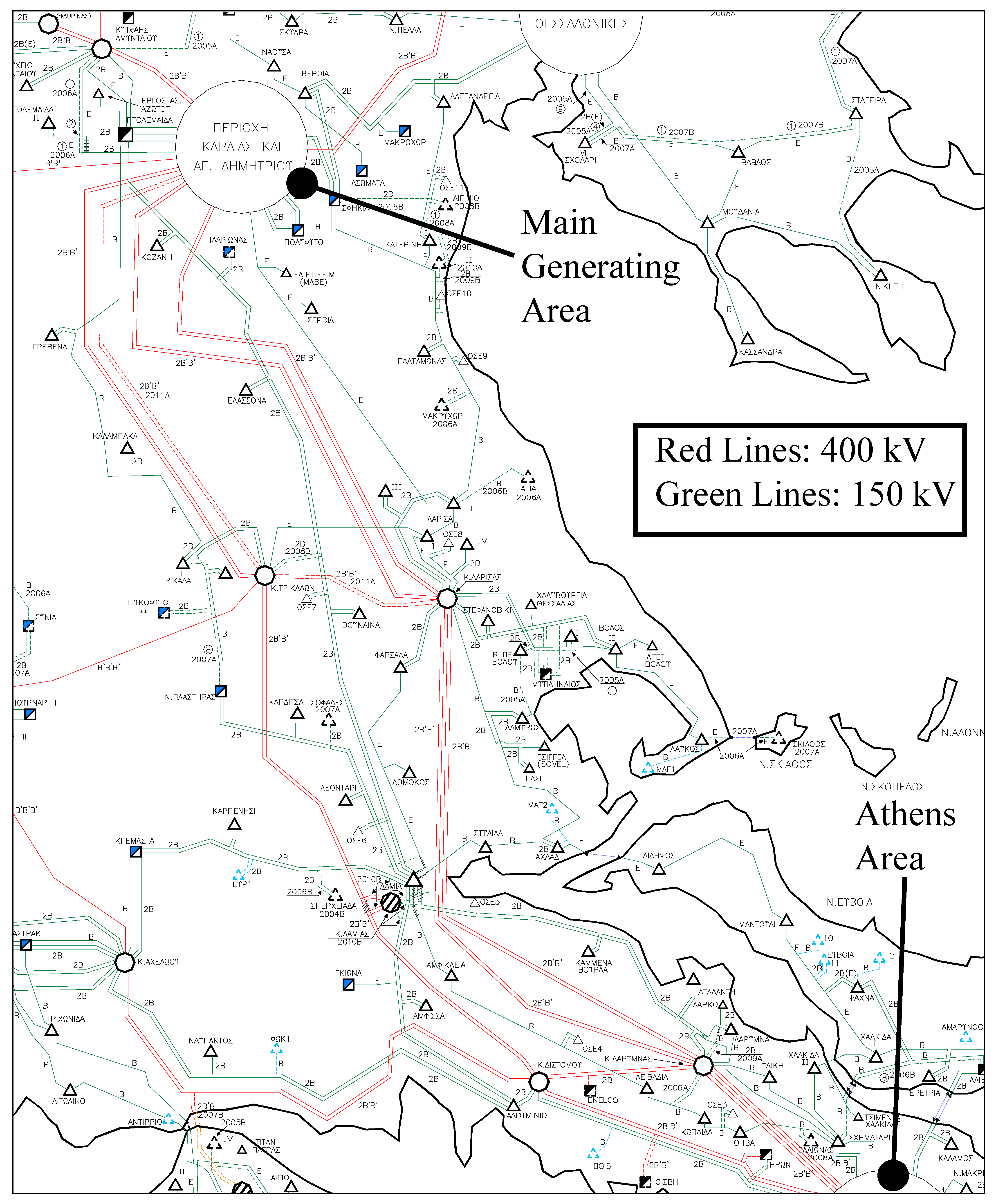
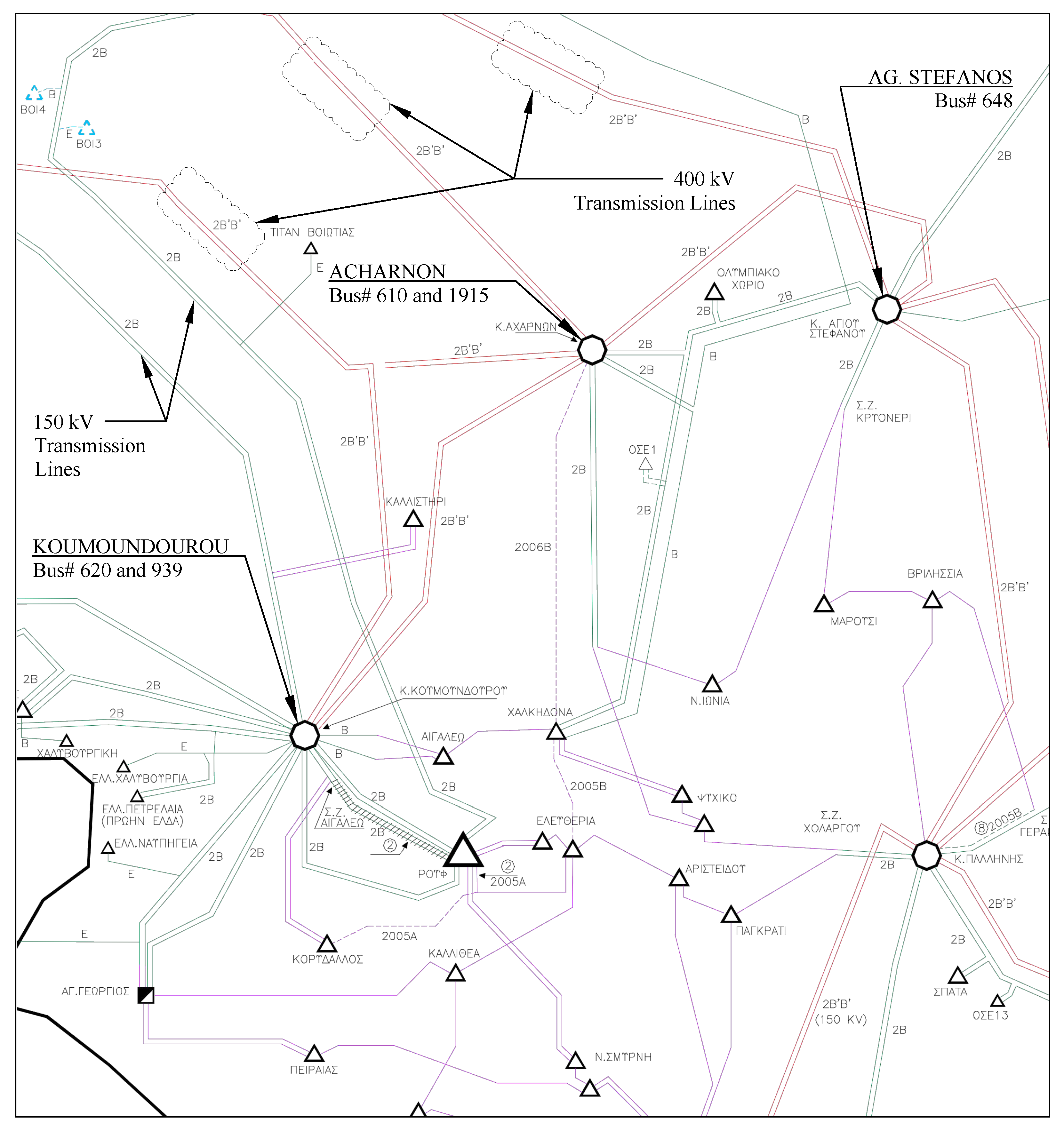
At the time of the July 2004 incident, the main generating area in the Hellenic Interconnected System was located at the northwest of the country, while the majority of the system load is concentrated at the southern part of the system, which includes the metropolitan area of Athens. Thus large amounts of power were transferred in the north–south direction, mostly by the 400 kV lines of EHV transmission system. These lines are shown with red in Figure 2, which includes a part of the Hellenic system. There are three, double circuit, EHV transmission lines connecting the buses shown in Table 1, which form a ring around Athens, as depicted in Figure 3.
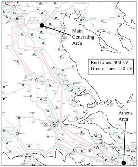
Figure 2.
North–south transfer corridor at 400 kV, shown with red color, Hellenic Interconnected System 2004.

Table 1.
Transmission lines and boundary buses of the 400 kV transmission corridor.
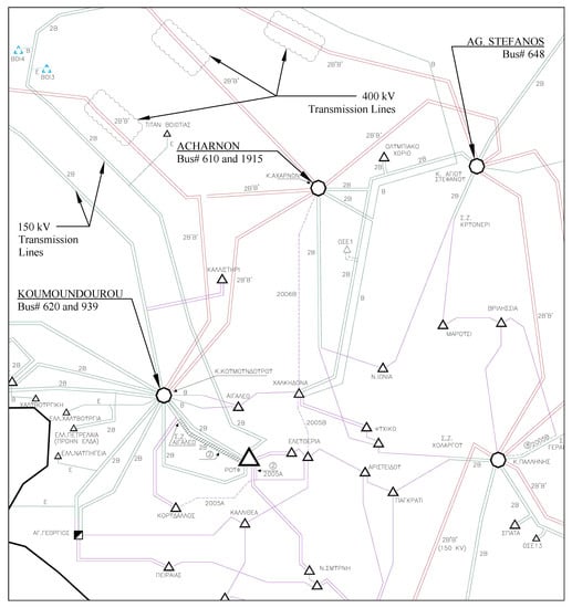
Figure 3.
The 400 kV boundary buses and respective corridor lines at the area of Attica, Hellenic Interconnected System 2004.
Even though there are also parallel HV transmission lines at 150 kV (shown with green in Figure 2), the main power transfer occurs through the aforementioned three double circuit EHV lines, which can be considered as the main transmission corridor to Athens and southern Greece.
It is assumed that PMUs and numerical relays able to compute RLI are installed at three EHV substations in the area of Athens (Table 1) and can be used for the computation of the relevant NLIs and RLIs, respectively.
For the particular case-study, apart from the voltage of each boundary bus, the receiving currents in EHV lines defined in Table 1 are also measured, in order to proceed with the calculations mentioned in Section 2.
The actual blackout sequence has been discussed in [19]. In this paper, with a view to create marginally stable and unstable scenarios, a slight modification is introduced to assess the sensitivity, the dependability and security of the voltage stability monitoring indices.
3.2. Modeled System and Derived Scenarios
For the evaluation of the voltage instability detection system two scenarios that differ in only one aspect are used. The first scenario is unstable, as in the actual blackout incident, while the second scenario is marginally stable. As stated above, these scenarios are meant to demonstrate the ability of the indices to distinguish between stable and unstable cases without issuing false alarms. Thus the incorporation of the detection system in an SPS will be reliable offering both dependability and security [5].
With respect to the original scenario, there are a few changes regarding the topology and the response of the system during simulation so that the case is made marginally unstable. More specifically, in this paper all EHV lines are connected while during the actual events of 12 July 2004 blackout, one circuit of the 400 kV lines connecting substations 395 and 1915 was open. Bus 1915 is also coupled to bus 610, at the same substation.
Regarding the response of the system during simulation it is assumed that all thermal units are equipped with automatic Armature Current Limiter (ACL). During the actual events, the reduction in armature current was performed manually by the unit operators.
As with the simulation of the original blackout [19], the initial operating point is considered the timestamp of 11:30, 12 July 2004, which corresponds to simulation time . At this point the total system load is 9084 MW, from which 1374 MW correspond to industrial load while 7710 MW correspond to end-user load. At the end-user load a constant uniform increase is applied with a rate per second from until .
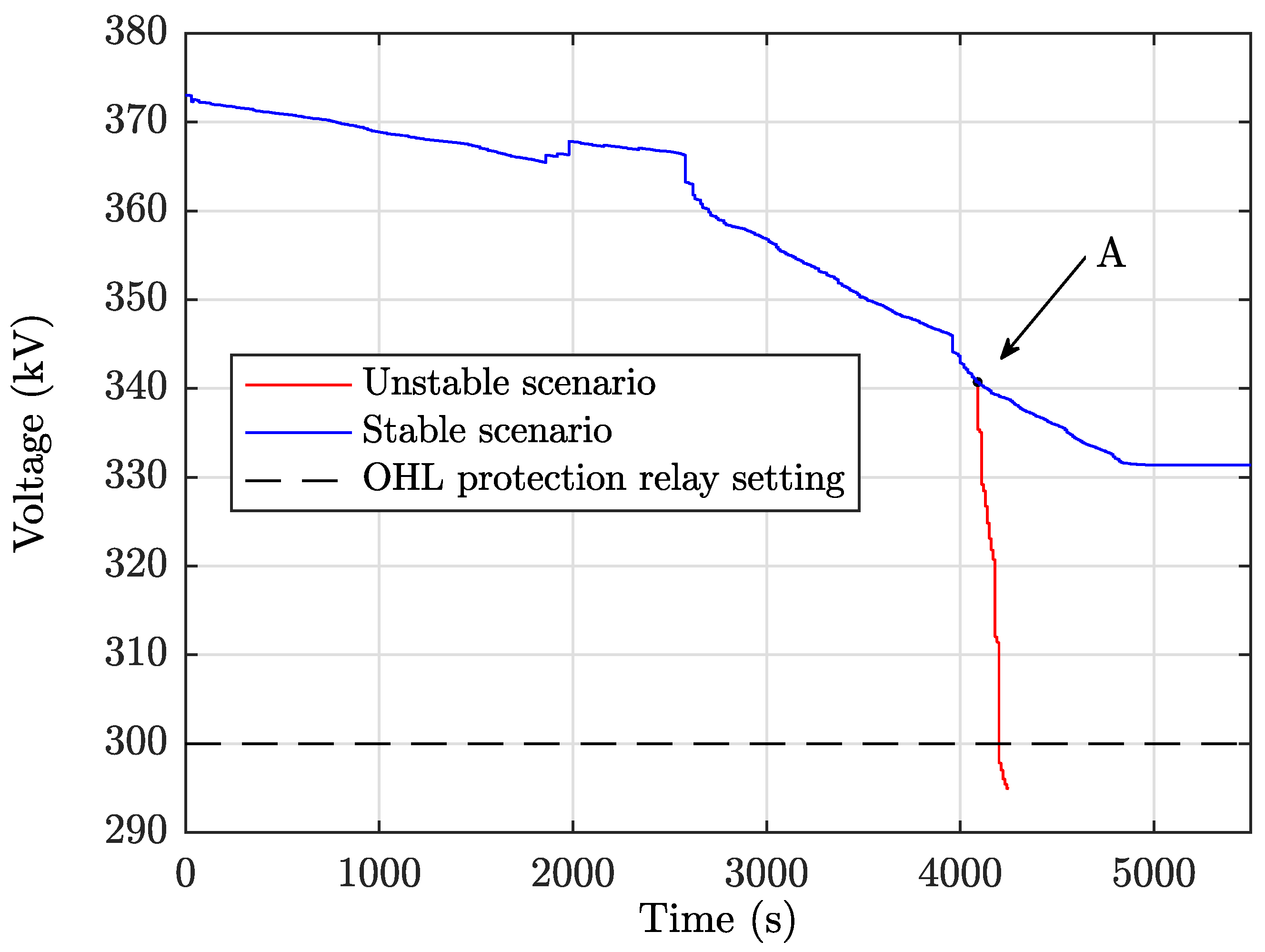
The only difference between the marginally stable and unstable scenario is the sudden loss of Aliveri III unit. In the unstable case, at the unit is disconnected, following which the system eventually collapses. In the stable case, the unit remains connected and the system reaches a new steady state with low voltages, but avoiding voltage collapse.
The above is evident in Figure 4 showing the response of EHV bus 620 for both scenarios. In the unstable scenario, point A signifies the instant where the unit Aliveri III is suddenly disconnected. This contingency deteriorates significantly the voltages of the southern system, since the corresponding unit is located near the metropolitan area of Athens, resulting in voltage collapse after 120 . In the stable scenario, the system reaches a new steady state approximately at , albeit with very low voltages. At this point it should be noted that the EHV transmission line protection relays have a function that trips the line when loaded above a certain level and with very low voltage. This was the relay function that opened the EHV lines during the last stage of the actual event. The voltage threshold for this function is set in the HIS to pu, This is shown with a dashed line in Figure 4. Thus, for the stable scenario, EHV line disconnection would be avoided.
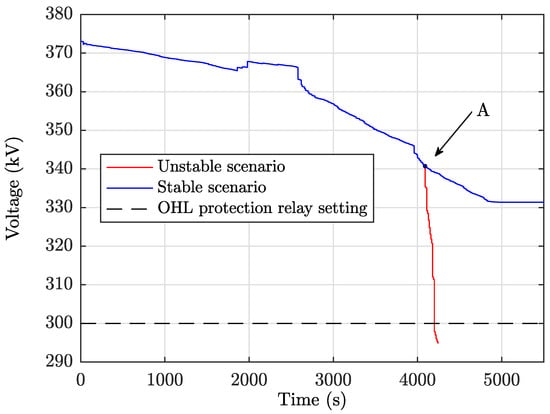
Figure 4.
Voltage response at EHV bus 620 (Koumoundourou). Point A: sudden loss of Aliveri III unit.
The calculation of NLIs and RLIs in both scenarios can be limited to receiving boundary buses 620 (Koumoundourou), 610 (Acharnon) and 648 (Ag. Stefanos). At this point it is highlighted that NLI and RLI indices at the receiving buses are identical, due to the fact that the topology on each receiving boundary bus consists of two identical parallel EHV circuits. Therefore, all figures containing the NLI time evolution also correspond to the RLI evaluated at each of the receiving end transmission line relays.
4. Simulation Results
4.1. Methodology
As stated already in Section 2, for the simulation of the Hellenic System and the application of NLI and RLI voltage instability detection indices (QSS approximation is used. This approximation replaces short-term dynamics by their equilibrium constraints [2]. Long-term simulation is performed using the WPSTAB software package, developed in NTUA. The long-term dynamics are represented by the Load Tap Changers (LTC) of bulk power delivery transformers [2]. The software package performs the long-term simulation and plots also regional and national PV curves, which show a representative bus voltage against system load.
The software package has also the option to form at each simulation step the Jacobian matrix of long-term equilibrium equations, assuming that the current operating point becomes an equilibrium by implying that LTC voltage setpoints become equal to their current voltage values. The so-formed long-term Jacobian is equivalent to the state matrix of the long-term dynamic system [2]. The dominant eigenvalue of this matrix is computed during simulation using the inverse iteration approach [2]. When the negative dominant eigenvalue becomes positive the system becomes voltage unstable. In parallel, the program can compute, also using the long-term Jacobian, the sensitivity of Q generation to additional Q demand. Alternatively, voltage instability can be monitored by the change of sign of this sensitivity through infinity [2].
The simulation step is set to and the voltage stability indices are calculated at time instants , that is, before re-evaluating the equilibrium point due to a discrete mechanism change (e.g. LTC operation etc.). In terms of modelling, the same assumptions as in [19] are followed regarding generator and load modelling.
4.2. Unstable Scenario
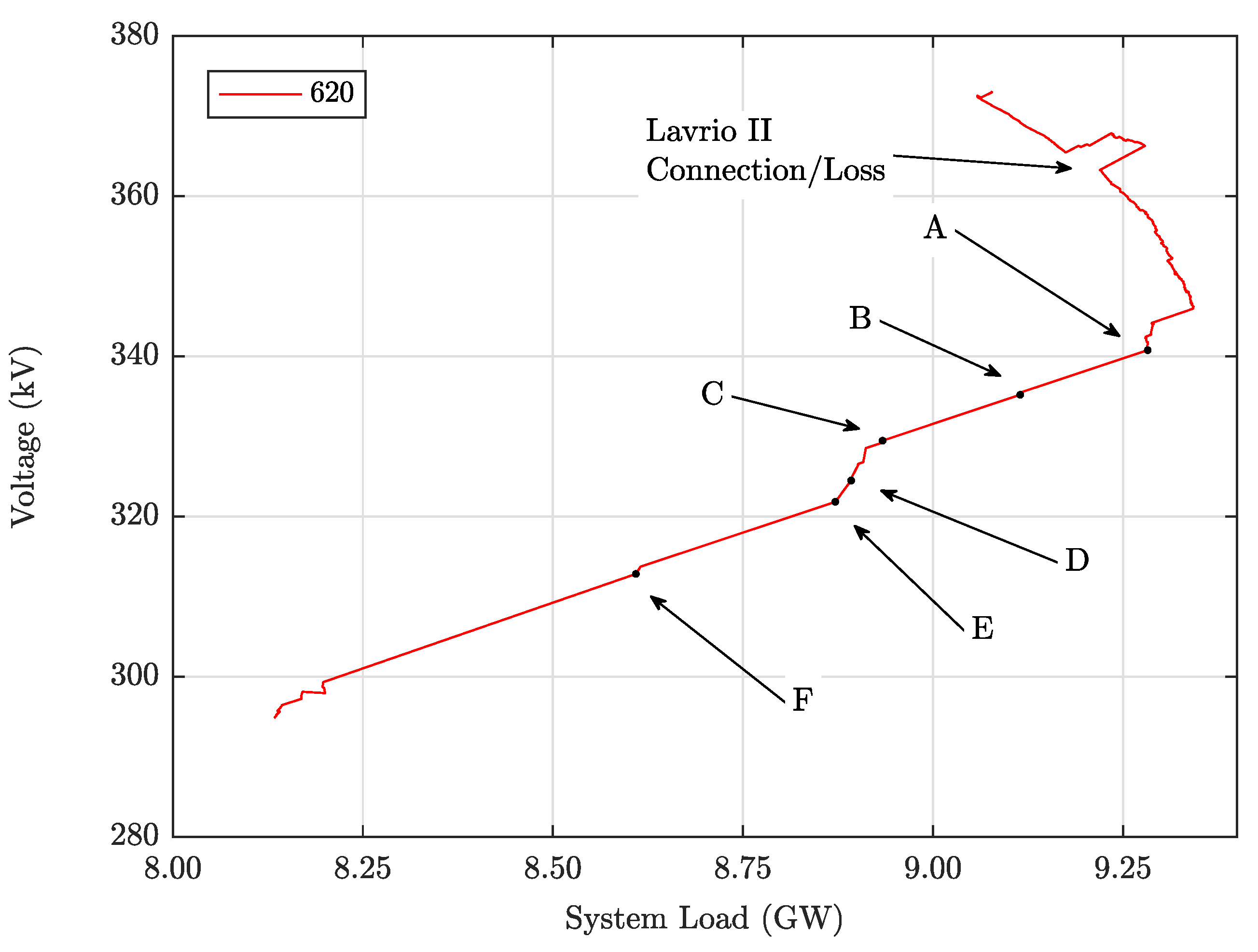
The unstable scenario, that is, the one including the loss of Aliver III unit is examined first. In this case, the sequence of major events are shown in Table 2, where the last column corresponds to points shown in Figure 5. The latter shows the national PV curve, which plots the voltage at 400 kV bus 620 versus the total load consumption in GW.
Table 2.
Sequence of events in unstable scenario.

Figure 5.
National PV curve (for bus# 620), unstable scenario. Letters A–F refer to Table 2.
From Table 2, it can readily be deduced that the OverExcitation Limiters (OELs) are activated in the majority of the generators of the southern system, leaving the area of Athens practically without voltage regulation, as seen in the national PV curve of Figure 5.
System deterioration is temporarily inhibited when the Lavrio II unit, located in the eastern part of Attica, is connected at , but its sudden loss during load pickup at brings the system again to an over-stressed state, as shown in Figure 5. From thereon, the continuous increase of system load activates more OELs, while the activation of ACLs ramps down the active generation of the thermal units near Athens, raising the need for additional remote active power dispatch towards Athens. At , the Aliveri III unit is disconnected (point A at Figure 5) followed by undervoltage trips of Aliveri IV (point B), Ag. Georgios 9 (point E), Lavrio I and Ag. Georgios 8 (point F) and finally the system collapses at .
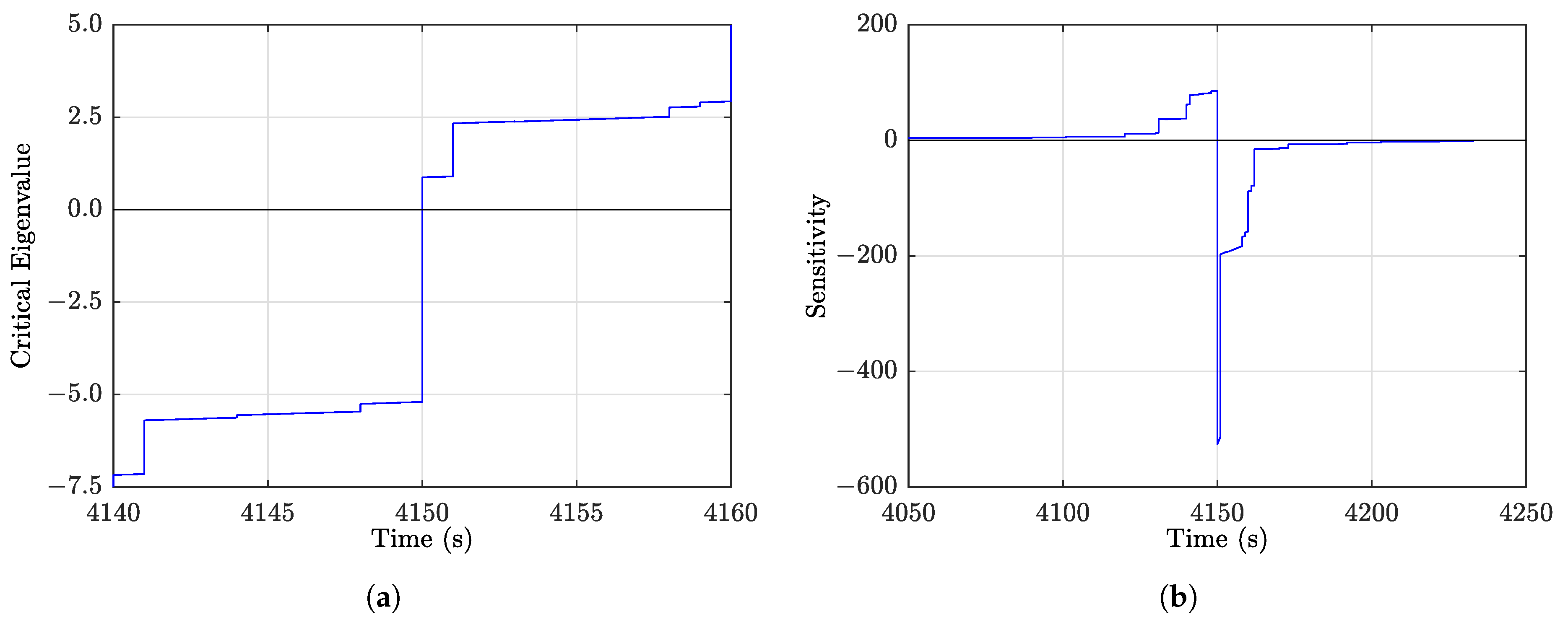
Voltage instability is reached at as determined by the calculation of the critical eigenvalue of long-term state matrix and sensitivity analysis, using the methodology described in Section 4.1. In particular, at this time instant, the critical eigenvalue of the unreduced long-term Jacobian matrix passes through zero, as shown in Figure 6a, while the sensitivities of total reactive generation to the reactive loads change sign from large positive to large negative, as shown in Figure 6b, which shows the response of the sensitivity corresponding to load of HV bus 737 at Piraeus.
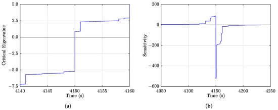
Figure 6.
Unstable scenario response of (a) critical eigenvalue and (b) Sensitivity of HV bus 737 at Piraeus.
Taking into consideration that the interval of 140 (between Aliverri III disconnection and system collapse) is very marginal for system operators to take load shedding decisions, an automatic load shedding scheme is mandatory in order to restore stability. Furthermore, it is also critical for a WAP system to timely recognize the point where load shedding has to be activated. As will be shown, both NLI and RLI indices perform satisfactorily in this respect giving an early warning in the marginally unstable case, without false alarm when the system is marginally stable.
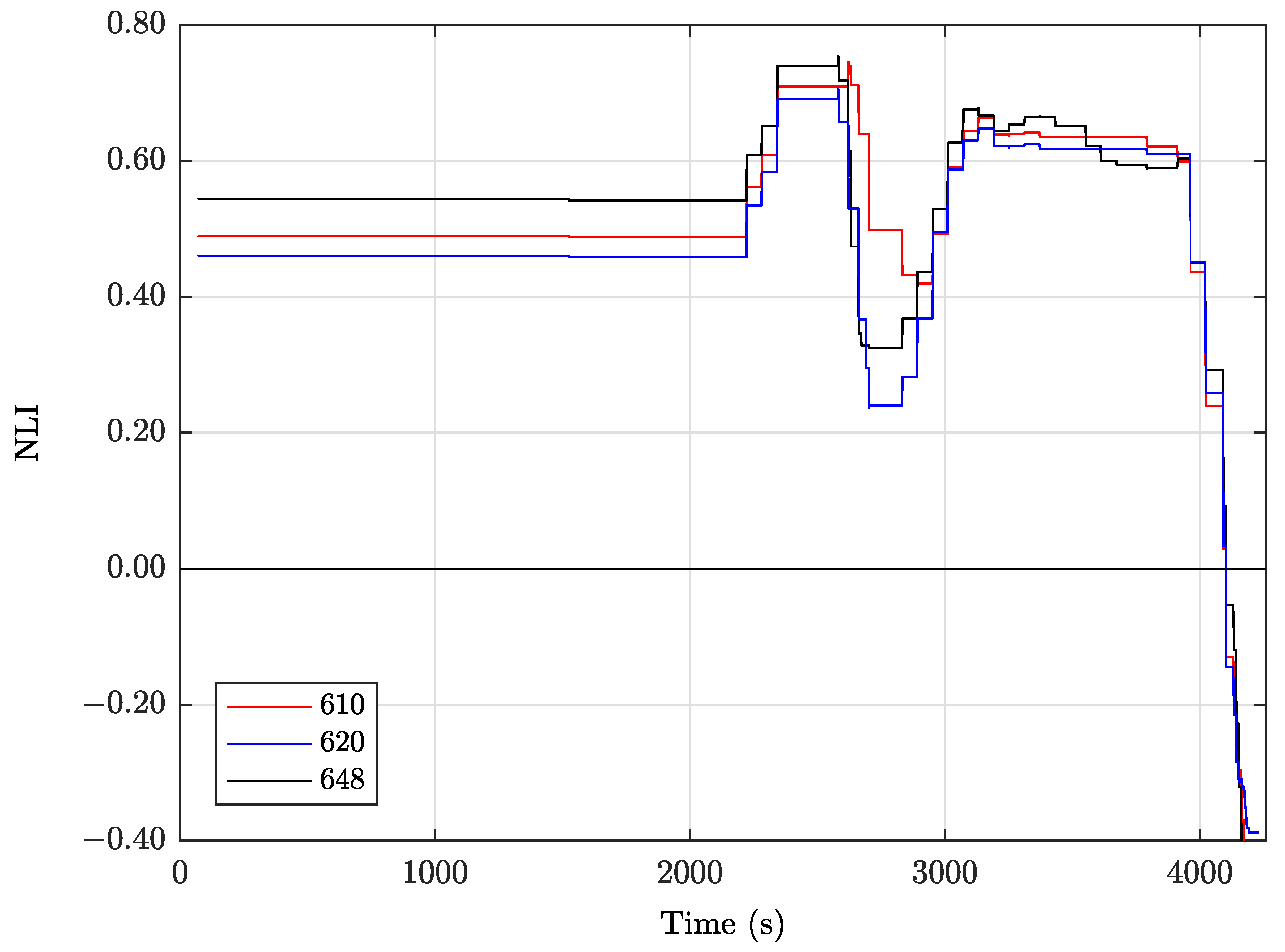
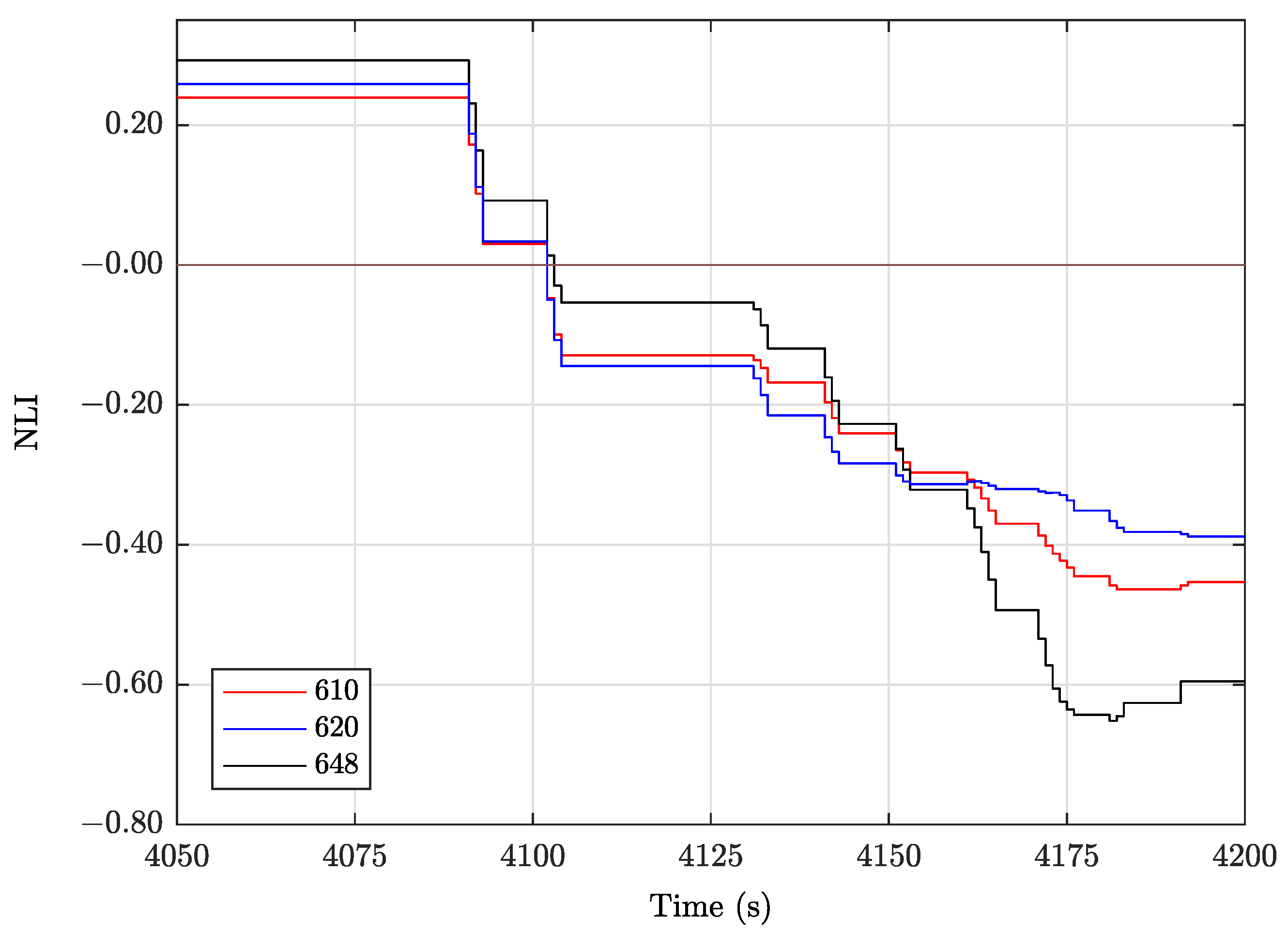
The NLI responses for the unstable scenario are shown in Figure 7 for each of the receiving boundary buses, while Figure 8 focuses on NLI responses close to the instability detection point. In Figure 8, it is readily observed that all NLIs become negative almost simultaneously. More specifically, NLIs change sign At for buses 610 and 620, while in the third substation, (bus 648) change of sign occurs 1 later (see also Table 2).
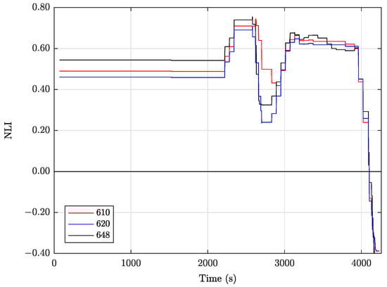
Figure 7.
NLI response at EHV buses 610 (Acharnon), 620 (Koumoundourou) and 648 (Ag. Stefanos), unstable scenario.
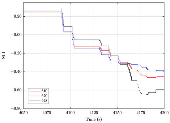
Figure 8.
Detail close to NLI change of sign, unstable scenario.
Thus, approximately 12 after the loss of Aliveri III unit the approaching instability is detected and corrective actions can be taken, since all NLIs and RLIs have become negative. It is noted that all indices change sign before the actual instability onset, but as has been shown in [17] this is expected, as the change of sign of NLI is expected to happen a little before the loss of stability. In this particular case, the time difference is less than 50 s and direct load shedding after this early warning is justified.
Another functionality that the RLI index may provide concerns the possibility of blocking undesired transmission line disconnection after the identification of voltage instability. Thus, an emergency trip-blocking signal could be activated at the relays whose RLIs have crossed zero, since the corresponding transmission lines are critical for stability.
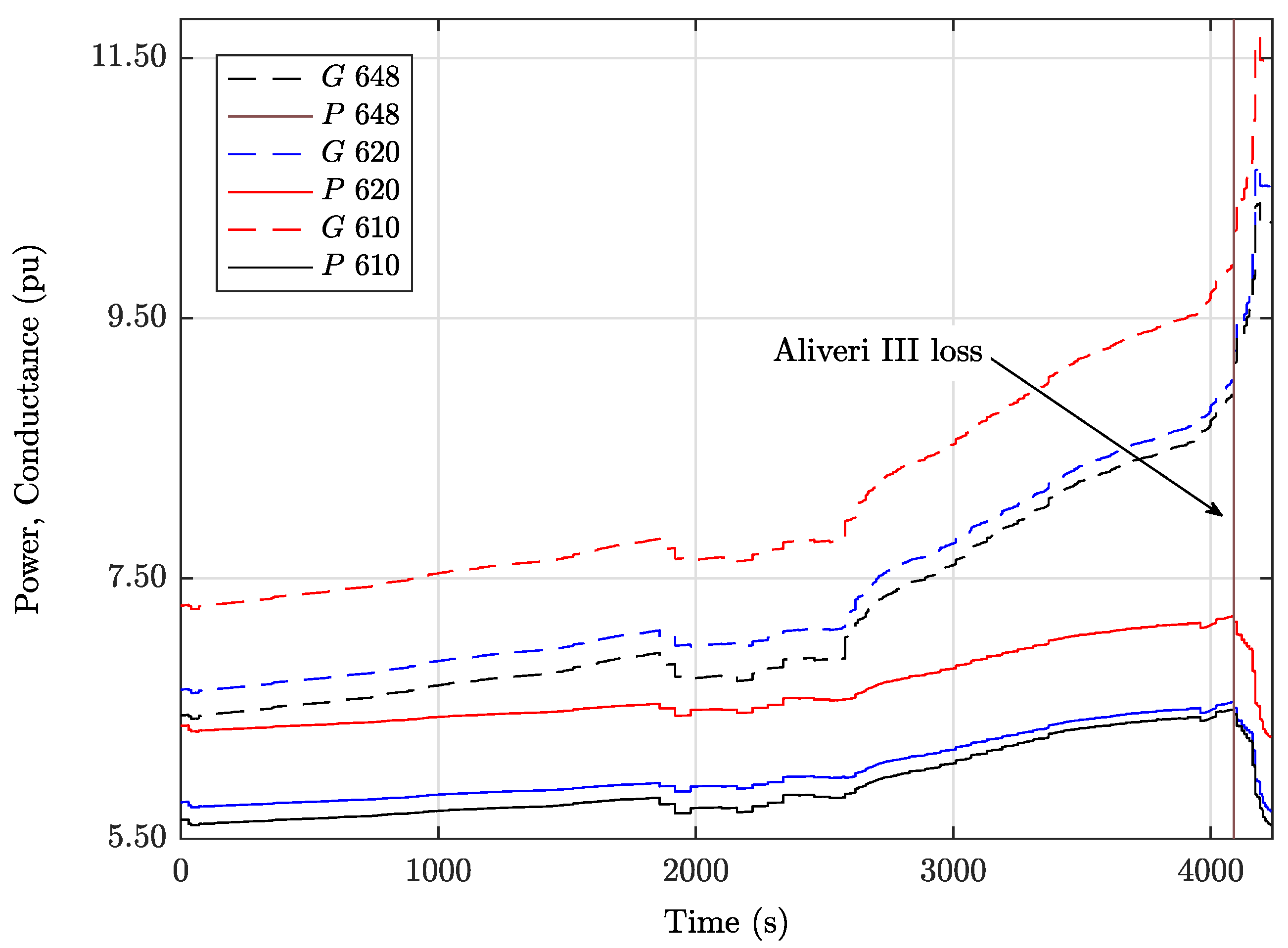
Figure 9 depicts the calculated apparent conductance G and received active power P for each of the receiving boundary buses. It can be observed that until Lavrio II unit connection time the apparent conductances maintain a relatively constant (and rather small) rate of change. At the time of Lavrio II connection, the system response is improved, as can be deduced from the EHV voltage evolutions in Figure 4 and Figure 5, as well as from Figure 7, where NLIs are seen to increase.
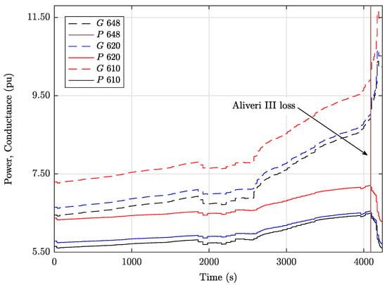
Figure 9.
Active power transfer and apparent conductance at EHV buses 610 (Acharnon), 620 (Koumoundourou) and 648 (Ag. Stefanos), unstable scenario.
After the Lavrio II unit disconnection at , the received active power increase becomes much slower than the apparent conductance trend, while after Aliveri III disconnection a sharp decrease in received active powers is observed, resulting in NLIs zero-crossing.
4.3. Stable Scenario
In this subsection, the stable scenario is simulated. The only difference between this and the unstable one concerns generating unit Aliveri III, which, this time, remains in operation. Thus, up to the point of Aliveri III trip (i.e., up to point A) the system evolution is identical to the one of the unstable scenario, as shown in Table 2, while from that point on, events for the stable scenario are shown in Table 3.
Table 3.
Sequence of events in stable scenario, after 4090 .
In this case, the system does not collapse and manages to reach a new long-term equilibrium point after approximately 84 min. Nonetheless, as will be shown, the new long-term equilibrium is very close to instability.
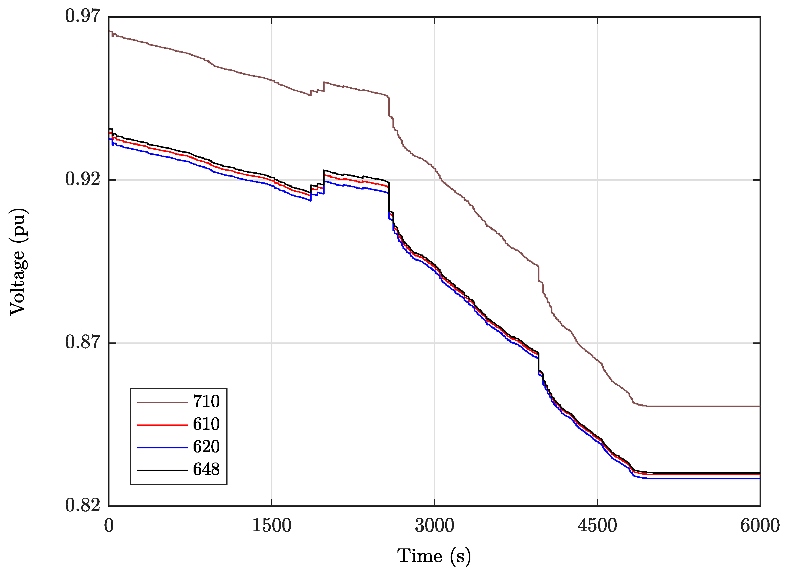
Figure 10 depicts the voltage responses of the three receiving boundary EHV buses, as well as of one representative HV bus. It can be observed that system voltages reach an equilibrium at around at a value close to pu for the EHV buses and pu for the HV bus. Therefore a considerable margin is assured and no undesired EHV line trips are expected to occur with the protection settings mentioned in Section 3 ( pu voltage threshold) during this stable scenario.
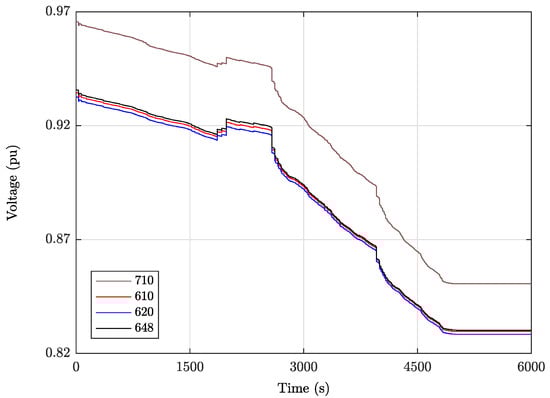
Figure 10.
Voltage response at Acharnon (610), Koumoundourou (620), Ag. Stefanos (648) and Rouf (710) substations, stable scenario.
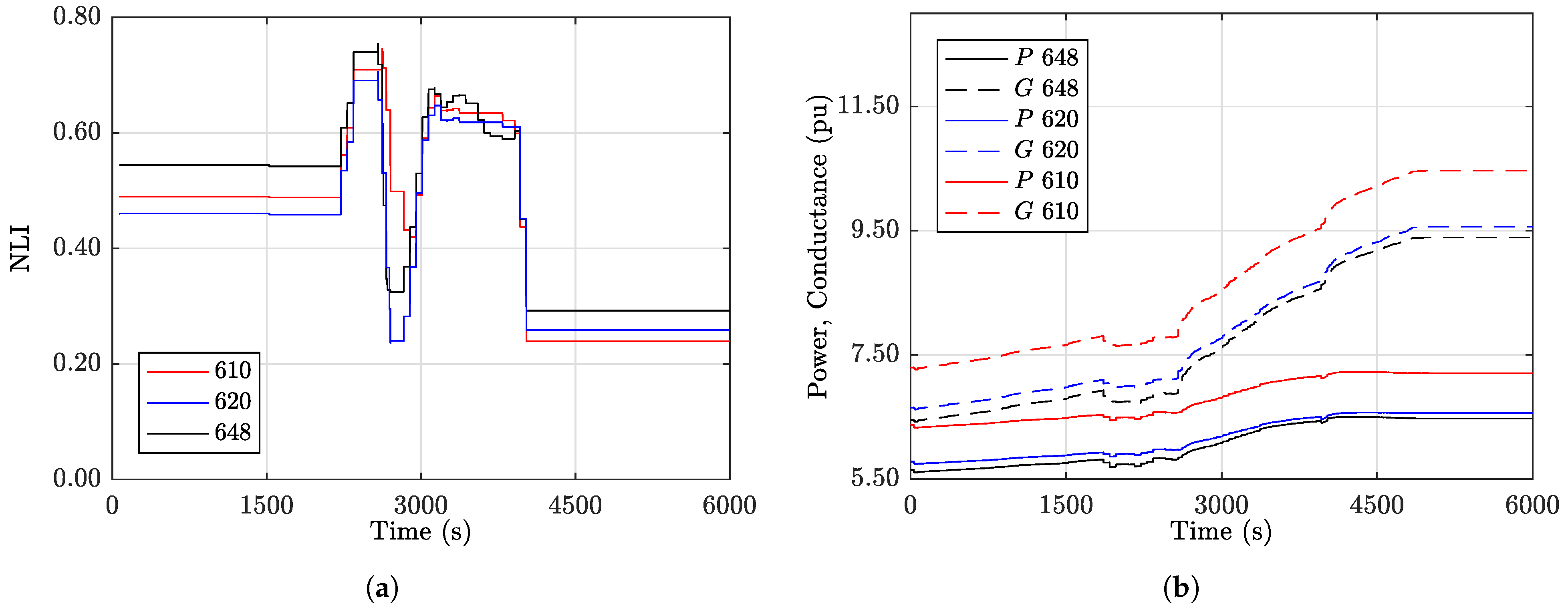
The NLIs (the respective RLIs obtain identical values) are presented in Figure 11a, while the corresponding apparent conductances and receiving active powers at the boundary EHV buses in Figure 11b. The considerably low NLI values at the end of the simulation indicate that the system has difficulty in delivering more active power to the receiving area of Attica, but is still stable.
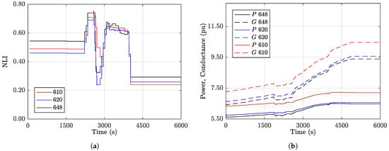
Figure 11.
Stable scenario response of (a) NLI response and (b) active power transfer & apparent conductance at EHV buses 610 (Acharnon), 620 (Koumoundourou) and 648 (Ag. Stefanos).
As can be seen, no false alarms are issued in the marginally stable case. Eventually, as LTCs reach their hard limits, load restoration is suspended, and after approximately as seen in Figure 11b, active power remains relatively constant. Thus, NLIs are no longer computed due to the filtering setpoint set in (4) and remain constant marginally below after .
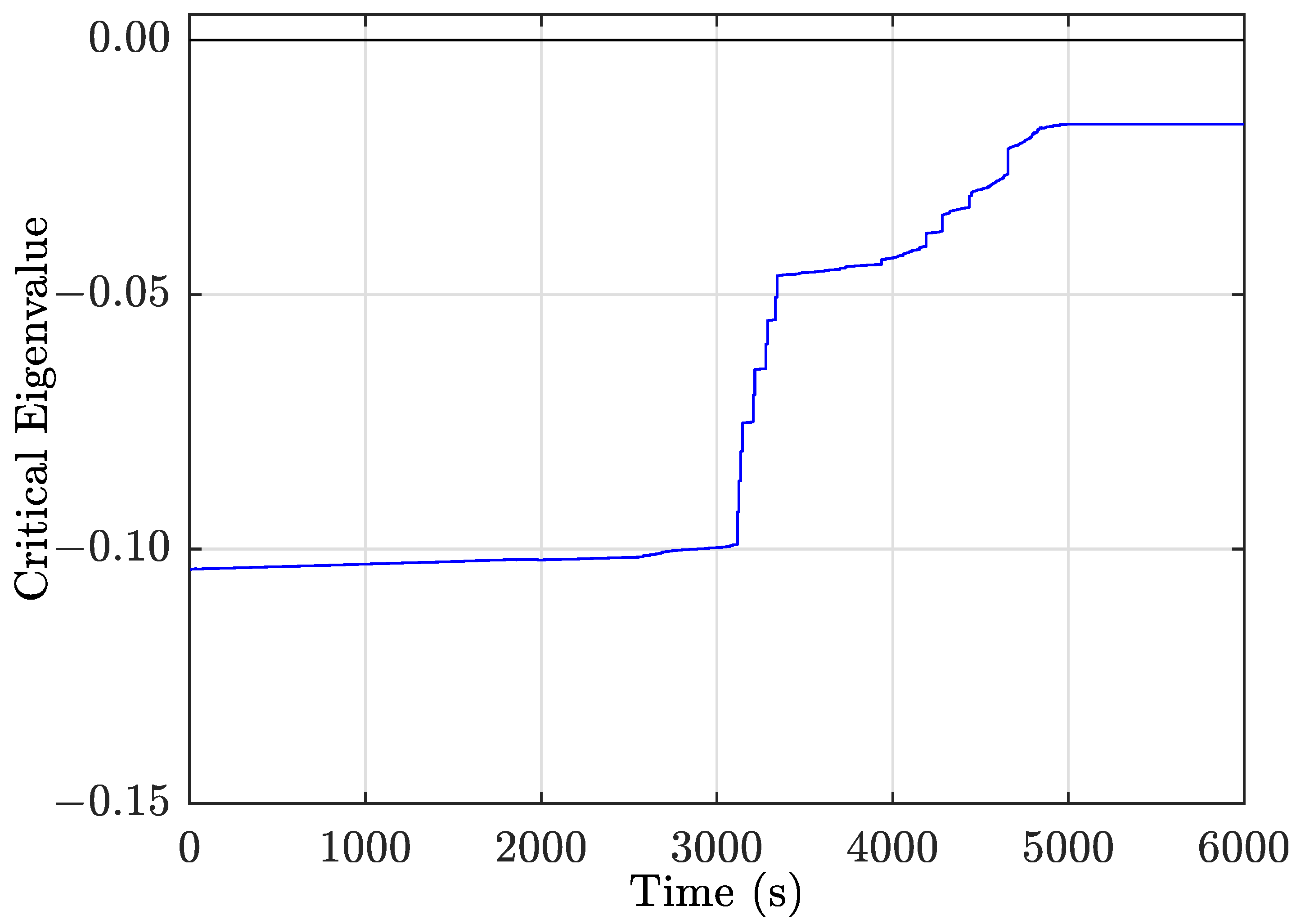
The fact that the system response is marginally stable is verified by the critical eigenvalue of the Jacobian of the long-term equilibrium equations (Figure 12), which continues to remain negative, although very close to zero, indicating that an additional system degradation will lead to instability. Taking into account that the system manages to remain marginally stable, there is no need to shed load, although corrective but non-intrusive actions by the operators are obviously required in order to enhance transmission system voltages, as they remain slightly above pu.
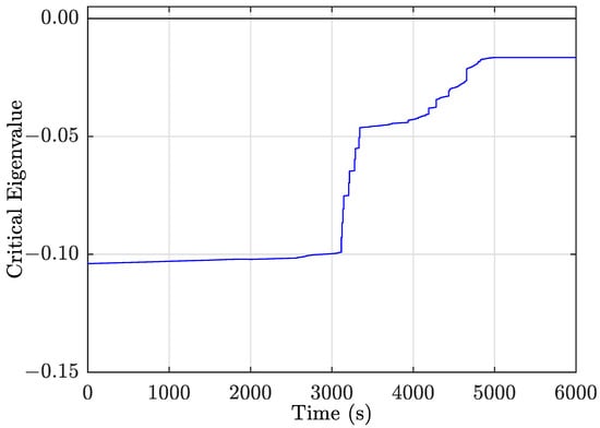
Figure 12.
Critical eigenvalue response, stable scenario.
This simulation has indicated the excellent performance and security of NLI and RLI indices. The very small final values where all indices have reached may also be used to raise the operator awareness to take further non-intrusive measures to improve the system and avoid further degradation and instability, for example, in case the load continues to increase.
5. SPS Application with Load Shedding
Having demonstrated the performance of the detection system in stable and unstable conditions, we incorporate it in an SPS, with direct load shedding in a set of predefined substations in the area of Athens.
More specifically, the SPS is designed to utilize the alarm from NLI/RLI voltage instability detection, when they become negative, and issue a 50% load shedding command to prespecified buses at three substations shown in Table 4. The bus nominal load powers shown correspond to nominal voltage. An intentional delay of 5 is set between the issue of the first alarm and the application of load shedding. This time interval includes also all communication or other activation delays involved.
Table 4.
Nominal load and available (50%) load shedding from substations in the area of Athens in 2004.
The load shedding scheme (close to 180 MW) applied in this simulation is very close to the one then available in the area of Attica, and was originally designed for the northern inter-tie protection. Other load shedding protection schemes were since designed (for instance [20,21]), but in this paper we concentrate on what was already in place at the time and could prevent the blackout, if only armed and automatically triggered by the NLI alarm.
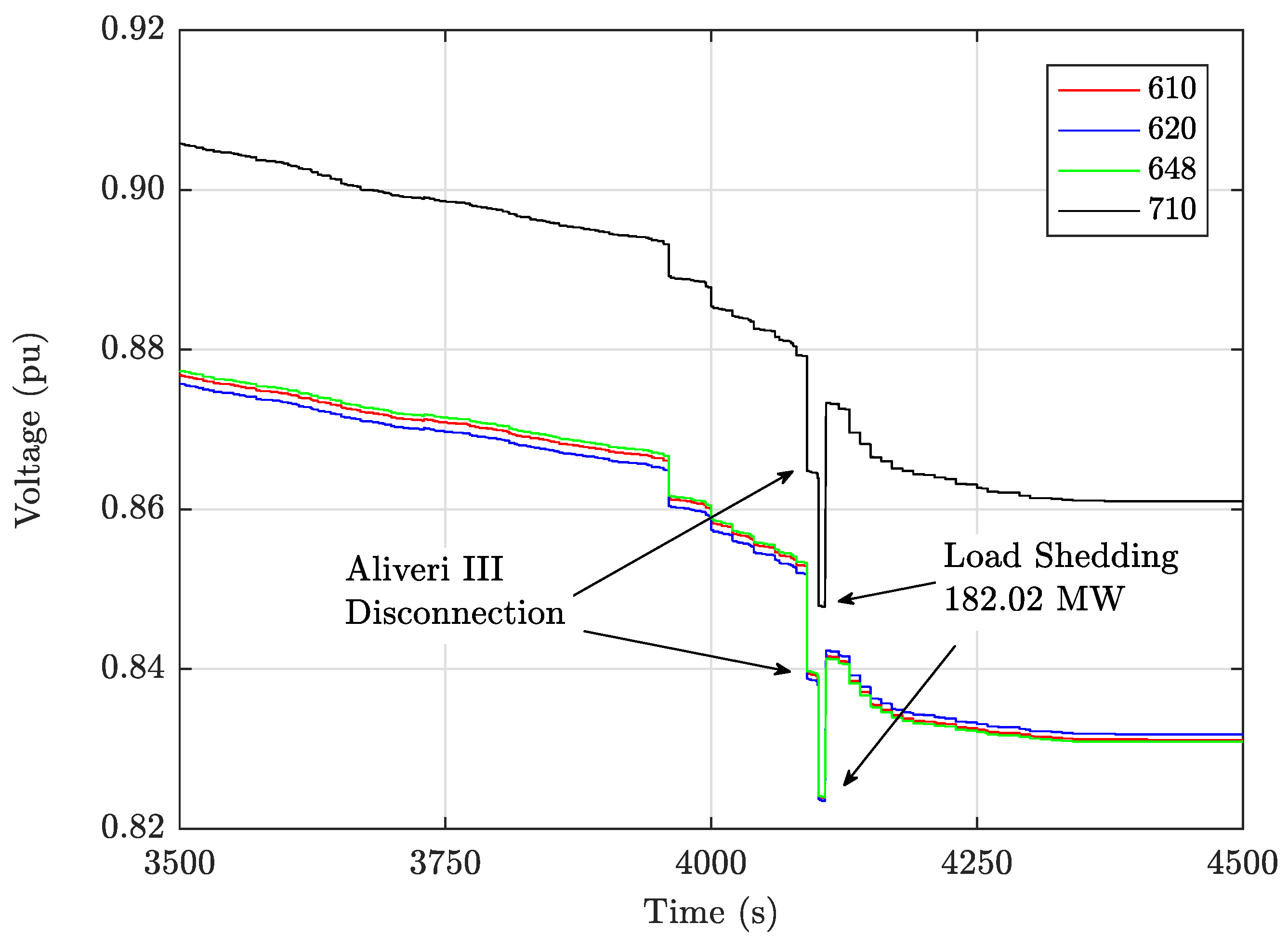
In order to demonstrate the performance of the proposed SPS we use the unstable scenario, where the first alarms are issued at . Following these alarms the load shedding is applied at with the nominal shed loads shown in the last two columns of Table 4.
The response of the power system after load shedding is shown in Figure 13, where the voltage response of the EHV buses 610, 620 and 648 and HV bus 710 is depicted. It is clear that the system is saved and reaches a new long-term equilibrium at with the voltages being above pu, with adequate margin from the transmission line protection relays voltage threshold mentioned in Section 3 ( pu).
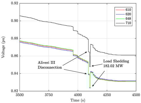
Figure 13.
Voltage response at EHV buses 610 (Acharnon), 620 (Koumoundourou), 648 (Ag. Stefanos) and HV bus 710 (Rouf) with the use of the proposed SPS and a load shedding of MW.
Since the application of load shedding is applied only when a voltage instability alarm is issued, the proposed SPS shows excellent performance in terms of dependability (acts only when needed), security (does not act when not needed) and thus is reliable [5].
6. Conclusions
In this paper, the simulation of a historical voltage instability incident in a real power system was used to validate the performance of a novel on-line instability detection approach. The simulated scenarios were derived from the July 2004 blackout of the Athens region in the Hellenic Interconnected System.
The voltage instability detection method assessed is based on the NLI and RLI indices, which are calculated from local voltage and current measurements acquired from transmission buses PMUs installed at the receiving-end boundary buses of the area prone to voltage instability. In this case the instability detection system was configured so as to monitor the main load center area of Attica, by independently calculating NLI and RLI indices at the receiving-end buses of the area’s main EHV feeding corridor. Furthermore, the simplicity of the detection system makes it attractive for incorporating it in an automated SPS with direct load shedding at predefined substations in the area of Attica.
Two scenarios have been investigated by means of QSS simulations, namely an unstable one, similar to the actual event, and a marginally stable one, with a view to assess the ability of the detection system to discriminate between unstable and marginally stable situations, therefore illustrating dependability and security. In the unstable case, the alarm was clearly issued very close to the actual point of voltage instability by all three instability indices independently. The timely identification of the impending collapse is crucial for the effectiveness of the applied remedial actions. In particular, it was shown that, by imposing a direct load shed of approximately 180 MW, collapse can be avoided and a new long-term equilibrium is achieved, albeit at relatively low system voltages, which call for further system restoration by the operators. On the other hand, in the stable scenario, no false alarm was issued and the system reached a new long-term equilibrium, for which most tap changers have reached their hard limits.
The excellent performance of the presented voltage instability detection and protection system opens the way for its actual implementation in a power system. This will allow secure system operation by providing a robust and adaptive system protection even for changing, more variable and less predictable operating conditions, for example, when large amounts of renewable energy sources are integrated in the system.
Future research will be focused towards implementing the indices in actual system operation and also on assessing the indices performance under unbalanced operating conditions. Finally, cases with a large penetration of distributed renewable generation will have to be considered in the near future.
Author Contributions
Conceptualization, C.L., P.M. and C.V.; methodology, C.V.; software, C.L.; validation, C.L. and P.M.; formal analysis, C.L. and P.M.; investigation, C.L.; data curation, C.L. and P.M.; writing—original draft preparation, C.L., P.M. and C.V.; writing—review and editing, C.L., P.M. and C.V.; visualization, C.L.; supervision, C.V. All authors have read and agreed to the published version of the manuscript.
Funding
This research received no external funding.
Institutional Review Board Statement
Not applicable.
Informed Consent Statement
Not applicable.
Data Availability Statement
Not applicable.
Conflicts of Interest
The authors declare no conflict of interest.
Abbreviations
The following abbreviations are used in this manuscript:
| EHV | Extra High Voltage |
| HIS | Hellenic Interconnected System |
| HV | High Voltage |
| LTC | Load Tap Changer |
| NLI | New LIVES Index |
| OEL | OverExcitaion Limiter |
| OHL | OverHead Lines |
| PMU | Phasor Measurement Unit |
| QSS | Quasi Steady State |
| RLI | ReLay-based Index |
| SPS | System Protection Schemes |
| UV | UnderVoltage |
| WAMS | Wide-Area Monitoring Systems |
| WAP | Wide-Area Protection |
References
- Taylor, C.W. Power System Voltage Stability; EPRI Power System Engineering Series; Mc Graw-Hill: New York, NY, USA, 1994. [Google Scholar]
- Van Cutsem, T.; Vournas, C. Voltage Stability of Electric Power Systems; Springer: Berlin/Heidelberg, Germany, 2008. [Google Scholar]
- Begovic, M. Undervoltage Load Shedding Protection; Technical Report, IEEE PES, Power System Relaying Committee, System Protection Subcommittee, Working Group C-13; IEEE: Piscataway, NJ, USA, 2010. [Google Scholar]
- Terzija, V. Wide Area Protection & Control Technologies; Technical Report, CIGRE Working Group B5.14; CIGRE: Paris, France, 2016. [Google Scholar]
- Van Cutsem, T.; Vournas, C.D. Emergency Voltage Stability Controls: An Overview. In Proceedings of the 2007 IEEE Power Engineering Society General Meeting (PES GM’07), Tampa, FL, USA, 24–28 June 2007; pp. 1–10. [Google Scholar] [CrossRef] [Green Version]
- Amraee, T.; Ranjbar, A.; Feuillet, R.; Mozafari, B. System protection scheme for mitigation of cascaded voltage collapses. IET Gener. Transm. Distrib. 2009, 3, 242–256. [Google Scholar] [CrossRef]
- Ramapuram Matavalam, A.R.; Ajjarapu, V. Sensitivity Based Thevenin Index With Systematic Inclusion of Reactive Power Limits. IEEE Trans. Power Syst. 2018, 33, 932–942. [Google Scholar] [CrossRef]
- Ospina, L.D.P.; Van Cutsem, T. Emergency support of transmission voltages by active distribution networks: A non-intrusive scheme. IEEE Trans. Power Syst. 2020. [Google Scholar] [CrossRef]
- Ospina, L.D.P.; Van Cutsem, T. Power factor improvement by active distribution networks during voltage emergency situations. Electr. Power Syst. Res. 2020, 189, 106771. [Google Scholar] [CrossRef]
- Cai, H.; Ma, H.; Hill, D.J. A Data-Based Learning and Control Method for Long-Term Voltage Stability. IEEE Trans. Power Syst. 2020, 35, 3203–3212. [Google Scholar] [CrossRef]
- Glavic, M.; Van Cutsem, T. Wide-Area Detection of Voltage Instability From Synchronized Phasor Measurements. Part I: Principle. IEEE Trans. Power Syst. 2009, 24, 1408–1416. [Google Scholar] [CrossRef] [Green Version]
- Glavic, M.; Van Cutsem, T. Wide-Area Detection of Voltage Instability From Synchronized Phasor Measurements. Part II: Simulation Results. IEEE Trans. Power Syst. 2009, 24, 1417–1425. [Google Scholar] [CrossRef] [Green Version]
- Rehtanz, C.; Bertsch, J. Wide area measurement and protection system for emergency voltage stability control. In Proceedings of the 2002 IEEE Power Engineering Society Winter Meeting. Conference Proceedings (Cat. No. 02CH37309), New York, NY, USA, 27–31 January 2002; Volume 2, pp. 842–847. [Google Scholar] [CrossRef]
- Liu, J.H.; Chu, C.C. Wide-Area Measurement-Based Voltage Stability Indicators by Modified Coupled Single-Port Models. IEEE Trans. Power Syst. 2014, 29, 756–764. [Google Scholar] [CrossRef]
- Milosevic, B.; Begovic, M. Voltage-stability protection and control using a wide-area network of phasor measurements. IEEE Trans. Power Syst. 2003, 18, 121–127. [Google Scholar] [CrossRef]
- De Villiers, F.; Donolo, M.; Guzmán, A.; Venkatasubramanian, M. Mitigating Voltage Collapse Problems in the Natal Region of South Africa. In Proceedings of the 36th Annual Western Protective Relay Conference, Spokane, WA, USA, 20 October 2008; pp. 1–9. [Google Scholar]
- Vournas, C.D.; Lambrou, C.; Mandoulidis, P. Voltage stability monitoring from a transmission bus PMU. IEEE Trans. Power Syst. 2017, 32, 3266–3274. [Google Scholar] [CrossRef]
- Nikolaidis, V.; Mandoulidis, P.; Vournas, C. Combining Tranmission Line Protection with Voltage Stability Monitoring. In Proceedings of the 2018 Power Systems Computation Conference (PSCC), Dublin, Ireland, 11–15 June 2018; pp. 1–7. [Google Scholar] [CrossRef]
- Vournas, C.D.; Nikolaidis, V.C.; Tassoulis, A.A. Postmortem analysis and data validation in the wake of the 2004 Athens blackout. IEEE Trans. Power Syst. 2006, 21, 1331–1339. [Google Scholar] [CrossRef]
- Nikolaidis, V.C.; Vournas, C.D.; Fotopoulos, G.A.; Christoforidis, G.P.; Kalfaoglou, E.; Koronides, A. Automatic Load Shedding Schemes against Voltage Instability in the Hellenic System. In Proceedings of the 2007 IEEE Power Engineering Society General Meeting, Tampa, FL, USA, 24–28 June 2007; pp. 1–7. [Google Scholar] [CrossRef]
- Nikolaidis, V.; Vournas, C. Design Strategies for Load-Shedding Schemes Against Voltage Collapse in the Hellenic System. IEEE Trans. Power Syst. 2008, 23, 582–591. [Google Scholar] [CrossRef]
Publisher’s Note: MDPI stays neutral with regard to jurisdictional claims in published maps and institutional affiliations. |
© 2021 by the authors. Licensee MDPI, Basel, Switzerland. This article is an open access article distributed under the terms and conditions of the Creative Commons Attribution (CC BY) license (https://creativecommons.org/licenses/by/4.0/).