Abstract
Apart from numerous technical challenges, the transition towards a carbon-neutral energy supply is greatly hindered by limited economic feasibility of renewable energy sources. This results in their slow and bounded penetration in both commercial and residential sectors that are responsible for over 40% of final energy consumption. This paper aims to demonstrate that combined application of sophisticated planning methodologies at building-level and presents incentive mechanisms for renewables that can result in prosumers, featuring hybrid renewable energy systems (HRES), with economic performance comparable to that of conventional energy systems. The presented research enhances existing planning methodologies by integrating appliance-level demand side management into the decision process and investigates its effect on the planning problem. Moreover, the proposed methodology features an innovative and holistic approach that simultaneously assess electrical and thermal domain in both an isolated and grid-connected context. The analyzed hybrid system consists of solar photovoltaic, wind turbine and battery with thermal supply featuring solar thermal collector and a ground-source heat pump. Overall optimization problem is modeled as a mixed-integer linear program, while ranking of all feasible alternatives is made by the multicriteria decision-making algorithm against several technological, economic, and environmental criteria. A real-life scenario of energy system retrofit for a building in the United Kingdom was employed to demonstrate overall cost savings of 12% in the present market and regulation context.
1. Introduction
Current trends and existing policies related to energy supply aim to alleviate global dependency on fossil fuels due to their finite nature and proven devastating effect on the environment. This led to the development of new technologies ranging from alternative and sustainable energy sources to innovative management solutions for available energy resources. Considering exploitation of renewable energy resources as the most prominent of them, many countries adopted suitable regulation and incentive mechanisms to improve the status quo and increase share of renewables in the overall energy mix. For example, the previous target set by the European Union (EU), which envisaged at least 20% of renewable energy sources in the final energy consumption by 2020, was recently updated to reach at least 32% share of renewables by 2030 (raised from 28% set previously) [1].
As part of this transition and in line with contemporary directives [2], buildings are increasingly being equipped with local energy sources and granted with capability to conduct individual energy management strategies, yielding a new entity in energy systems referred to as prosumer. However, ensuring a widespread transition from consumers towards prosumers depends on the economic viability of renewable energy sources and accompanying equipment. Although renewable energy sources are already a relatively mature technology, prosumers are still facing significant issues regarding upfront investments, making it hard to level up with the cost-effectiveness of conventional energy supply from coal and gas. Aiming to overcome this issue and spark the necessary widespread adoption of renewable technologies, national governments implemented various incentive programs and mechanisms such as feed-in or generation tariffs, carbon credits, tax refunds, and procurement subsidies tailored for each type of renewable technology. All these measures share a common goal to alleviate the economic impact of associated capital and operational expenditures. In doing so, they intend to make the overall investment profitable on the long run and render the transition from conventional to renewable sources viable for consideration. Apart from instantaneous effects to present investments, these incentive programs also contribute to a decrease of manufacturing costs of renewable energy technologies in the long-term by scaling up the overall number of installations. Besides various financial incentive mechanisms, economic performance of prosumers can also be improved with application of innovative energy management technologies. They not only increase operational efficiency of renewables but also contribute to increased reliability and availability of energy supply in the context of multisource hybrid renewable energy systems (HRES). Given the intermittent nature of renewable energy sources, the latter becomes increasingly important as the transition to renewables in urban areas also needs to meet very high availability and quality of energy supply standards. Therefore, to establish a cost-effective and reliable prosumer, one would need to asses two fundamental aspects:
- (a)
- The planning/dimensioning problem, which represents an optimal rated power split of different renewable sources and storage capacities within prosumer systems, resulting from a multicriteria decision making process against complex objectives combining maximization of economic performance, environmental neutrality, and independence from the power grid.
- (b)
- The operation problem, which focuses on optimal energy management strategy for a given prosumer and its energy assets. Moreover, it considers optimization of prosumer’s energy imports and exports as well as internal power flows between multiple renewable/conventional energy sources and storages against multiple technological, economic, and environmental criteria.
As reviewed by [3], there are many commercial software solutions that aim to solve different individual aspects of these two problems while offering different types of outputs (high-level efficiency or economical parameters, dynamic operational values, etc.). However, although seemingly independent from each other, the two are intrinsically correlated as the decision on optimal prosumer energy assets is impacted by their day-to-day management and, ultimately, reached through a long-term simulation of its operation.
The considered planning problem was extensively investigated starting from standalone HRES in isolated rural areas, where there was a lack of conventional energy supply to those grid-connected, as the penetration of local energy sources in urban areas became more significant. Following is a brief overview of more recent research efforts dealing with such planning problems and related optimization approaches. An approach for both stand-alone and grid-connected modes using the energy filter was discussed in [4], while [5] proposes a multicriteria decision analysis for PV-WT grid connected systems. A research effort conducted on HRES in the form of a microgrid system in [6] incorporates the addition of a battery energy storage systems (BESS) and employs two procedures, a source sizing and battery sizing algorithms in sequence. Scalfati et al. [7] proposes a mixed-integer linear programming (MILP) based solution for sizing that can, in its general form, be used for different microgrid architectures and storage technologies. Sizing with sensitivity of a microgrid structure specific for a university campus is discussed in [8], while optimal sizing with implemented DR strategies is discussed in [9] where a HRES configuration is considered. HRES optimizations with regards to energy, economic, and environmental indicators can also be found in [10] where a multiobjective optimization was employed to determine the best system configuration. The authors note that no single system configuration can simultaneously satisfy the selected three criteria and proposes the selection of a trade-off Pareto optimal solution. Economic parameters and capital investment benefit analyses can also be found in [11] where optimal sizing and power management of prosumers equipped with PV was considered using a two-step approach, with the first step analyzing the technical model (short-term assessment resulting in outputs such as component sizing and battery lifetime), and the second one tackling the long-term assessment through economic modeling. The authors report that an increase of profitability by up to 14% was achieved. Finally, a stochastic approach using MILP for determining optimal sizes of prosumer assets (PV generation capacities and batteries) is proposed in [12]. The authors describe a methodology that minimizes the joint combination of investment, maintenance, and operational costs in different scenarios that result in varying energy consumption levels from the grid.
Regarding the optimization problem, various different techniques can be found in the related literature. As the proposed methodology includes a proactive approach based on utilization of demand-side management (DSM), and in line with findings from a systematic review from [13], the most prominent technique for this type of problem is linear programming (LP) with its mixed-integer variant being the one most commonly used. For example, ref. [14] proposes a multiobjective mixed integer linear programming (MOLIP) technique to facilitate residential DSM in a system where effects of storage systems are specifically analyzed. Also, ref. [15] formulates a MILP model to be used for optimizing profit on the electricity market of a system with photovoltaic (PV) panels and BESS. These optimizations are performed for a horizon of 24 h with hourly varying prices. This model does not consider load to be appliance-based but rather views it as an aggregate value. Also, since the simulation is performed for a short amount of time, the monetary investments and maintenance costs of running such a system are not considered. Paper [16] continues with a MILP model also employed for a 24 h simulation horizon but with a shorter, 15 min-long sample period. The modeled system considers optimal appliance scheduling with a PV source present, with load scheduled on a per appliance basis. The results were obtained and discussed for both single and multiuser scenarios. However, the investment and maintenance costs related to running a renewable energy source are also not considered. The framework laid out in [17] also implements a MILP model for optimal appliance scheduling during a 24 h horizon with a 15 min sampling period. The chain rule, defining that a given appliance can only be started after another one finishes its operation, is introduced. The model output is discussed for three scenarios in a specific use case: a fixed price tariff, a variable price tariff with ripple control (devices that switch on or off appliances based on the current tariff), and a variable price tariff with optimal scheduling. Concluding that, because of the insignificant difference in the applied price tariffs, it would not be viable for an average domestic consumer to look for a solution more sophisticated than ripple control. The authors also state integrating distributed generation and storage into the model as a future research point. Finally, ref. [18] focuses on optimizing energy management of a residential microgrid with the goal of analyzing the relation between the level of demand flexibility and cost savings. This paper also models investment, maintenance and replacement costs of BESS as well as distributed PV and wind turbine (WT) generators, and it introduces a discreetly operated appliance whose operation can be split into multiple nonconsecutive time periods. Considering that this system uses a relatively lengthy, one-year-long horizon with a sample rate of 1 h, the model is designed on an efficient window-based concept. Nonetheless, this approach does not considered load to be appliance-based, i.e., specific appliance activations cannot be traced in the final results. Also, a notable addition with this paper is that the sizing problem is solved simultaneously with scheduling using the appropriate variables implemented in the model. Although this is a very efficient way to solve such a problem, the linear programming paradigm constrains those variables in a linear way, and thus, limits the modeling potential to a certain extent.
Finally, building upon previous research and aiming to improve the current state of the art, this paper proposes the introduction of a two-step optimization process that jointly considers the planning and operation problems. As will be described in greater detail in the following section, the inner loop optimizes operation of individual configurations using the available load shifting mechanisms while the outer loop explores key performance indicators for each of these configurations and selects the one that adheres best to the desired preferences. The remaining part of the paper is organized as follows. Section 2 presents the proposed planning methodology and description of the optimization process as a whole. Section 3 unveils the mathematical implementation of both operation and sizing models supported by Appendix A which outlines the models used for simulation of renewable technologies (RET). Section 4 describes the employed real-life use case scenario for methodology testing and verification, while Section 5 discusses the obtained results depending on the desired criteria. Lastly, Section 6 provides concluding remarks and conclusions. The paper is also supported by a nomenclature table in Appendix B that contains the list of all abbreviations and variables used.
2. Proposed Planning Methodology
The overarching objective of this paper is to demonstrate that by combining sophisticated methodologies for planning and operation of prosumers leveraging small-scale residential HRES and existing governmental incentives for renewable technology, one can retrofit or even completely replace conventional energy supply without making a compromise regarding economic viability of such transition. In other words, the presented research aims to mitigate the economic barrier associated with global uptake of renewables by demonstrating cost-effectiveness comparable to that of conventional energy sources. Moreover, the considered real-life use case scenario exhibits the possibility to even exceed it in the context of existing long-term incentive programs and country-specific energy regulations.
To reach this objective, a novel planning methodology for future prosumers was established by leveraging the benefits of increasingly utilized mechanisms of DSM. In particular, the underlying approach exploits load elasticity, both in time and intensity, to reduce capital investment in renewable energy technologies, improve their economic performance and increasing overall penetration in energy supply portfolio. In addition, the proposed decision making process simultaneously assesses multiple consumer-defined criteria presented in Section 2 and Section 5. The techno-economic performance of viable configurations is discussed in the latter section, where the effects of the proposed planning methodology are evaluated in the most conspicuous way. Moreover, the proposed methodology assumes a holistic approach for the planning process, which simultaneously considers both electrical and thermal domains. Although previous research mainly assessed these two domains separately, they are inevitably cross-correlated, especially in cases when thermal demand is satisfied through a heat-pump, which combines any available thermal source (e.g., ground, solar, or air) and a proportional amount of electricity, as described in Appendix A. Moreover, such consideration is even more relevant in cases where thermal demand is satisfied from several different sources, (e.g., gas, electricity, or solid fuels). Following a theoretical elaboration, the proposed methodology is demonstrated through its practical application in a real-life scenario featuring actual technical, economic, and environmental constraints.
The proposed HRES planning methodology, developed to devise an optimal system topology as well as sizing of its individual components, aims at fundamentally enhancing existing planning tools and algorithms by combining different approaches and adding new design aspects. In short, it introduces and brings together the following aspects:
1st. The overall HRES planning process considers simultaneously both electric and thermal energy demand, while current approaches typically consider electric or thermal domain, exclusively, with the methods for such optimizations previously discussed in [19]. Employed methodologies therein are focused on balancing the selected demand type with available energy sources, conversion elements, and storages. However, increased utilization of devices like heat pumps, which satisfy the thermal demand while contributing to electricity demand, requires a holistic assessment approach. The differences between the traditional approach and the one proposed by this paper is illustrated in Figure 1.
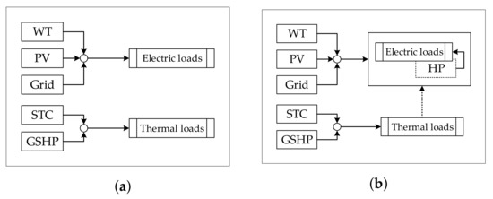
Figure 1.
Two approaches for demand modeling. (a) Traditional approach. (b) Proposed approach.
2nd. The most utilized approach to consider isolated (island) HRES deployment scenarios is extended towards consideration of grid-tied deployment, which brings a more dynamic context where varying import and export energy prices are applied and unlimited energy exchange with power grid is enabled.
3rd. The increasing application of DSM programs and, more specifically, DR schemes in day-to-day operation is considered on an appliance level and corresponding implications on the planning of HRES and dimensioning of individual components are evaluated.
4th. MCDMA is employed to rank feasible HRES topologies with capabilities of simultaneously evaluating a wide range of technical, economic, environmental, and societal design criteria.
In the following elaboration, each design alternative will be referred to as HRES configuration, which is defined with a set of discrete sizes for each RET components. Hence, the configuration will consider both the HRES topology and sizing of the energy assets within.
The optimization process can be split into use case evaluation and two main distinct sections: operation optimization and sizing optimization, as presented in Figure 2. Firstly, in the evaluation stage, the values like demand profiles, financial information and RET parameters are collected and fed into the model. A set of predefined HRES configurations deemed fit for the selected use case is defined, and when it comes to the definition of the search space for the optimal HRES configuration, a set of context-defined and user-defined constraints is established. The following list summarizes the most influential design constraints into several categories, which are simultaneously assessed by the proposed methodology to deliver optimal HRES topology and sizing:
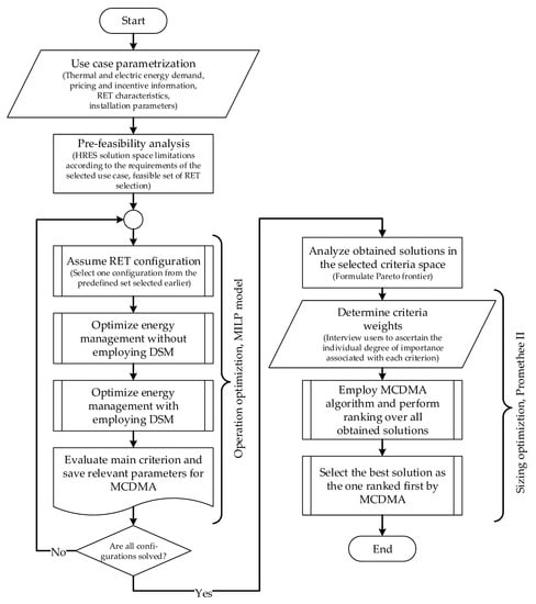
Figure 2.
Optimization process flowchart.
- Renewable energy sources (RES) harvesting potential (solar irradiation data, wind data, ambient temperature, ground temperatures);
- Building characteristics and space availability constraints (indoor area (basement), outdoor area, roof, wall facades, surrounding area);
- Energy demand requirements and flexibility (electricity demand, heating/cooling demand, hot water demand);
- Dynamic energy pricing (dynamic import/export energy prices, feed-in tariffs);
- Financing conditions (budget/loan, cost of capital, governmental incentives, inflation, increase of energy prices);
- RET equipment characteristics (photovoltaic panel, wind turbine, solar collector, geothermal heat pump, auxiliaries (DC/DC, DC/AC), battery storage, boiler);
- RET installation parameters (wind turbine installation height, azimuth and elevation of photovoltaic panels, etc.)
The listed constraints, in fact, define a set of boundaries for the space in which the optimal design solution is searched for. The operation optimization stage is initiated by equipping the model iteratively with one of the predefined alternatives.
2.1. Operation Optimization
The underlining structure of the system that was selected for operation optimization and is implemented in this study is a solution proposed in [20], referred to as the Energy Hub, with its general structure illustrated in Figure 3. It represents how the input power vector () is transformed in several stages (denoted by matrices for input transformation, C for conversion and for output transformation, as discussed in Section 3.1) while also managing storage charge/discharge rates ( for the input storage stage and for the output storage stage), exported power () and loads (L).
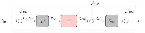
Figure 3.
General structure of Energy Hub.
Given the variability of generation from renewable sources, energy demand requirements, and dynamically determined energy costs, each feasible configuration is modeled and its long-term operation is simulated and optimized. When deciding on the simulation time horizon and size of the time step resolution, several factors were taken into account. Firstly, long-term performance of an HRES is heavily influenced by the renewable energy harvesting potential, which implies utilization of historical meteorological conditions for a given location. Moreover, since the performance should be evaluated for the entire HRES lifetime, which is typically around 20 years, the so-called typical meteorological year (TMY) data, which provides hourly data for typical meteorological conditions over a relatively long period and, thus, objectively characterize the specific geographical location, was selected. Secondly, given the objective of long-term assessment of HRES operation, the linear (or mixed integer) models of energy assets running on hourly resolution are sufficiently complex. Consequently, hourly resolution was chosen as the time step while the time horizon is one-year- long. However, long-term performances can be extrapolated by multiplying these results as many times as needed. This is due to the methodology natively taking into account events such as replacement of an asset (e.g., batteries typically last for 5 years) or time-limited governmental incentives (e.g., payment periods of 7–20 years for RET subsidies).
The operation aspect of the described model is finished once all the predefined HRES sizing configurations are optimized and their internal variables saved for later processing in the sizing segment.
2.2. Sizing Optimization
Finally, when the iterative simulation procedure of the inner loop is concluded, and the list of evaluation criteria is derived for each configuration, it is necessary to establish appropriate ranking among the configurations, considering multicriteria (multidimensional) evaluation space. To do so, an existing MCDMA algorithm was employed for this segment, previously called the outer loop.
At the initial stage, the MCDMA is fed a list of alternatives A, which ought to be simultaneously ranked across multiple criteria C. Each alternative A, represented by an individual HRES configuration, is first individually evaluated across the whole range of criteria C, referred to as evaluation criteria in the dynamic performance assessment elaboration. Following is the assignment of the weighting factors w to each criterion C. These weight factors allow for non-uniform distribution of the level of importance assigned to each criterion, allowing end user to practically steer the selection process according to desired needs and preferences. Following the findings from [21] noting its common applications for technology evaluation, the acknowledged performance ranking organization method for enrichment evaluation (Promethee) II algorithm [22] was utilized for the purpose of development of MCDMA functionality, as described below.
Firstly, a comprehensive pair-wise comparison is calculated as
Afterwards, those differences are passed through a preference degree function where can be defined in a variety of ways, with the most common being a linear variant
bounded by and . Every pair of actions is compared using a multicriteria preference degree
where a constant to weights is applied
After calculating
a net value is calculated . Finally, ranking all alternatives according to gives a complete ranking considered as the output of the Promethee II algorithm.
The proposed methodology can easily consider different design criteria, which can be summarized into four general categories. In the following list, these categories are out-lined with detailed elaboration of each category that was implemented and its items following later in the text:
- Technical criteria: Loss of Power Supply Probability (LPSP), Wasted energy
- Financial criteria: Capital Expenditure (CAPEX), Operational Expenditure (OPEX), Net Present Value (NPV), Internal Rate of Return (IRR), Payback Period (PP)
- Environmental criteria: greenhouse gas emissions (CO, NOx, SOx)
- Social/Economic/Political criteria: Fuel Reserve Years, Job creation, Inter-country energy dependence etc.
3. Mathematical Model
The key feature of the proposed methodology is the model implemented to facilitate the optimization process and, just like the process itself, the mathematical model can be represented with two sets of parameters, one depicting operation and one depicting sizing optimization.
3.1. Operation Optimization
Generally, a MILP problem is defined as determining a vector of variables
that minimizes a certain objective function f which is usually written as
Meanwhile, the vector must also adhere to a set of conditions that are split into four categories: equality and inequality constraints, lower and upper bounds and integer constraints. If a subvector of x is defined as
and the lower bound and upper bound vector as
these constraints can be written as
The vector of variables x is formed by arranging a set of all variables required for the model at every instance of the simulated time horizon like
If is used to denote the sample rate of the model, for any of the variables in may denote the value of at the k-th time sample, i.e., Since some of these variables should incorporate values for different types of electric energy sources (WT, PV, and electricity from the grid), they are natively multidimensional. However, for computational modeling, x must be a row vector, hence these natively multidimensional variables are flattened out in a predefined order. For example, given a simulation time horizon of , the variable holds instantaneous imported power values for WT if values for PV if and values for grid electricity if Therefore, for modeling purposes, it may be convenient to think of such variables as matrices in a reshaped form. Regarding our example variable we may consider a three-by-one native vector where is the corresponding instantaneous imported power from the WT, is the corresponding instantaneous imported power from the PV array and is the corresponding instantaneous imported power from the grid, all calculated at Obviously, every matrix equation that employs such variables in their native shape can be easily converted to a vector based expression required for MILP implementation. Thus, for the sake of clarity, variables from the vector x will, in the remainder of this paper, usually be written in their native form abbreviated as with an index k referring to the instance of time at which the variable is being evaluated. For the sake of clarity, the index k is omitted when a variable is referenced in text, but is present in all formulas where that variable is used.
3.1.1. Energy Balance
The instantaneous imported power can be from either the WT, PV array, or the grid and this power can either be stored at the input level or dispatched to the rest of the system through the appropriate transformers. The law of conservation of input power states that the balance
must hold. The power sent to the storage unit is converted into energy via
The available energy of the storage unit is determined by an integral expression
with an initial condition as defining the SOC in the first sample, and is usually set to zero if optimizations on consecutive time intervals are not being performed on the same system. The energy not being stored at the input is sent to the conversion stage defined as
The output of the conversion stage can then either be exported back to the grid or further dispatched to the output stage. This is simply written as
with exporting power which was previously imported from the grid back to said grid being directly prohibited by
where is a matrix that determines which carrier is to have a fixed (restricted) export and sets those values. The power not being exported is then sent to the output transformation stage that aggregates the carriers into an arbitrary number of values depending on the number of load types. This operation is performed in the equation
Analogous to the input, the output can also feature a storage option. The charge/discharge rate is obtained from
Similarly to the input stage, the output storage SOC is calculated by
and an initial condition is given as which concludes the set of equations governing the energy balance of the energy hub system. Furthermore, additional equations must be added for load management mechanisms.
3.1.2. DSM and Load Variables
To properly allow the model to perform necessary optimizations, some auxiliary features must be introduced as constraints. First of all, load L can either be attributed as fixed load which cannot be optimized in any way or flexible load which can used for optimizing by means of time shifting (shiftable load), splitting its operation into multiple time instances (dispersible load) and adjusting its instantaneous power consumption (elastic load). Nevertheless, for every appliance we define an on/off state variable that is defined by
The flexible load at the k-th time sample can be written as
with the total load being expressed as
However, the product being summed in (22) would represents a nonlinear operation between two variables and so it must be rewritten. To achieve this, is divided into three components: nominal power draw, positive power deviation, and negative power deviation from the nominal value, or in other words
Nevertheless, (24) also incorporates a product between variables, however and will be constrained to having nonzero values only when the appliance is turned on, this expression can be reduced to
Finally, total load can be expressed as
Since is set beforehand, this expression is actually a linear combination of variables (subvectors) from x, and can therefore be implemented as a MILP constraint. According to the classification laid out in [23], elastic loads can be classified either as being either energy-based meaning that they must consume a predefined amount of energy within a specified time window or comfort-based meaning that they must control an environmental variable within a desired range. With effects of DSM on comfort-based appliance being previously investigated in [19], this paper will focus only on energy-based elastic appliances for DSM with an option to elastically adjust their power within given bounds. Therefore, for each appliance, a set of windows (activation cycles) is defined with one of them, a vector
defining the n-th window of i-th appliance by having nonzero values equal to n at time instances that belong to that window. This implementation allows for windows that need not be continuous, i.e., they can be split into an arbitrary number of segments. Since these windows are also predefined like the nominal power, they can be used for forming an energy constraint
stating that a specified appliance i must only be active a given amount of times so that the amount of energy it spends during that activation cycle n is equal to the product between nominal power and the length of nominal activation belonging to that window. Because power deviations also affect the energy consumption, it is also stated that the sum of power deviations must be equal to zero during a given window, or in other words
thus finalizing the set of equality constraints required for the model. Nonetheless, these relations are not sufficient for the model and some additional conditions must be applied in form of inequalities.
3.1.3. Auxiliary Constraints
Because a set appliance should not have a nonzero positive and negative power deviation at the same time, two variables are introduced to indicate when these deviations are active by defining
with the constraint
prohibiting simultaneous positive and negative nonzero deviations. Additionally, defining another constraint
in combination with (31) forces the indicators to have a correct sign. Finally, by specifying
a link between the deviations and their respective indicators, and thus, forcing these variables to uphold the definition set by (30) was provided. To allow for an easier implementation of the results obtained from this model and to facilitate load dispersion penalization in the objective function, another variable called the device start indicator is introduced by
marking that the device i will be turned on in the following time sample. Since this definition describes a nonlinear relation between and the proper values for are obtained by simultaneously enforcing three inequality constraints
This same indicator is also used to allow for modeling both dispersible and nondispersible appliances by specifying
and concluding the primary set of equalities and inequalities for the model.
3.1.4. Variable Bounds
To supplement the equality and inequality constraints stated previously, a set of bounds in posed for the variable vector All of the instantaneous values of power must be non-negative, and thus, the following bound is imposed
On the other hand, the imported power must be equal to the available amount provided by the renewable sources at all times if considering those respective elements, or unbound if considering elements describing the import from the grid. Therefore,
At both the input and output stages, storage levels must be between the lowest possible (zero) and highest possible (battery capacity) SOC and so
with and being limited by
where is the highest achievable charge rate, and thus, also bounding and The total load L only has a defined lower bound equal to the value of fixed load since the flexible load is non-negative, and thus
As mentioned before, both deviations and also have bounds equal to a predefined upper and lower deviation limit, respectively, applied during specified windows as follows
As for the indicator variables, the device start has a lower bound of zero and upper bound of one for all time samples, i.e.,
while the on/off state has the same bound within windows and both bounds set to zero outside
A similar logic is employed as to limit the deviation indicators
Finally, since the indicator variables should only assume a value of either zero or one, thus rendering this problem to be classified as MILP rather than LP, we specify
3.2. Objective Function
Depending on the effect that is desired to be achieved, different objective functions can be formed. Relevant literature most commonly considers cost minimization, discomfort minimization, and maximization of on-site generation use. These criteria can also be combined as to create a mixed objective and so one such possibility is considered
3.2.1. Cost Minimization
One of the most frequently considered parameters when discussing feasibility of renewable generation systems is the monetary cost that ultimately falls on the end consumer. To model the effects that running a HRES has over the simulated horizon, the prices of energy attributed to imports and exports is taken into consideration. The active cost of running such a system can be calculated with
Factors and usually represent zero or negative values because the use of renewable generation is generally subsidized by governments and their values, like the values of other factors in (47), vary depending on local regulations and acting price tariffs. Therefore, the parameters of such a cost function are use case dependent, and their exact values will be discussed later on in the paper.
3.2.2. Dispersion Minimization
Sometimes, splitting one appliance’s operation cycle into several disjointed segments may be considered as unwanted behavior impacting user’s comfort. To combat this behavior for dispersible appliances, a criterion is defined as
Minimizing such a function by itself would lead to no appliance utilizing dispersion, hence, a combined criterion may be used and is implemented in the proposed solution to simultaneously balance minimizing cost and penalizing unwanted load dispersions.
3.3. Sizing Optimization
As mentioned previously, the second part of the proposed methodology, besides the optimal management of energy resources accomplished by the MILP solver, is determining the proper configuration of the site, also referred to as the sizing problem. Since multiple combinations of available renewable generators and storage options are being considered, a set of criteria is selected to facilitate MCDMA ranking of all available configurations with the first one being optimal with regards to the specified weights associated with each of the given criteria.
3.3.1. Total Cost (EMI)
Since the model application considered in this paper will mainly focus on residential users, the total cost of running a renewable project is one of the most important factors to be considered when ranking different configurations. The yearly cost relating to importing and exporting energy is expressed by (47). However, this relation does not take into account initial investment costs, maintenance and eventual replacement costs associated with using equipment with a finite life span that may malfunction during its operation. To assess all of these expenses in a comprehensive way, equated monthly installments and maintenance costs are calculated. For a piece of equipment labeled i one month’s equated installment (equivalent to rent) would be equal to
where . The corresponding criterion for the MCDMA can now be written as
with symbolically denoting all of the devices for which the costs need to be included.
3.3.2. Net-Zero Energy Building Rating
The concept of net-zero energy buildings (NZEBs) gained a lot of prominence lately and its importance was also recognized by several governments with the EU’s Energy Performance of Buildings Directive (EPBD) even requiring all new buildings from 2021 to be at least near-zero energy (nZEBs) [2,24]. A NZEB is defined as an energy efficient, self-sufficient structure which roughly consume the same amount of energy as it produces on site over the course of a year. With around 40% of global energy consumption being attributed just to buildings, such a concept of energy management and planning is set to greatly improve the current environmental effects of powering buildings in the near future. To facilitate a balance necessary for a NZEB or nZEB rating, we may consider minimizing the criterion
where is the amount of power consumed or stored and is the amount of power generated on site by either the WT or PV for each time step.
3.3.3. CO2 Emissions
Finally, to quantify the impact that running the operation of the considered system has on the environment, the total mass of CO may be considered. This criterion can be simply calculated as
4. Use Case
To display the capabilities of the proposed methodology, a concrete use case is assumed in form of a simulated residential household property located on the Ravenscliff Road in Motherwell, Scotland, United Kingdom (GPS coordinates 55.80, −3.96) shown in Figure 4, located around 25 km from the center of Glasgow.

Figure 4.
Considered building and corresponding installations. (a) Property. (b) STC and PV installations.
4.1. Energy Hub Model
The considered system, with its appropriate Energy Hub structure presented in Figure 5, has three different types of input electric energy: WT generated, PV-generated, and grid-imported. No thermal energy is taken into account because the thermal load is considered to be met by the STC and GSHP and is observable trough the fixed electric load generated by these systems as will be described later. Also, the raw imported energy cannot be stored in any way, and therefore the appropriate matrices required for input storage modeling are
The imported energy is directly dispatched to the conversion stage so
Since the user only pays for the active power measured by the local meter, as not to interfere with the objective function calculation, is assumed while some losses may incur when converting power from renewables, and thus, was set, which is a common inverter efficiency value. Moving on, users with distributed generation such are WT and PV are allowed to export excess energy back to the grid. However, exporting electricity imported from the grid is prohibited with
performs an aggregation of all three types of energy carriers at the output stage as only electric loads exist in the model. The output stage features a single storage unit for electric energy, and therefore

Figure 5.
Implemented structure of Energy Hub.
4.2. Tariff Information
The address of the proposed use case is located in an area with the supply code 18 named “South Scotland” meaning that its energy is supplied by ScottishPower. Although several tariffs are provided by ScottishPower with varying prices between them, those differences are mostly negligible, and Online Fixed Saver December 2019 [25] tariff was selected with the consumption costs at and for electricity and gas respectively, and daily standing charges at for both energy carriers.
Residential users in Great Britain can take advantage of a Feed-in tariff (FIT) scheme administered by the Office of Gas and Electricity Markets (OFGEM). Although feed-in tariffs usually refer to an amount paid just for exporting energy back to the grid, a generation tariff is also offered. With related numbers changing every three months, the generation tariff scheme available for new applicants at the time of writing this paper is for accredited PV installations smaller than and for WT installations smaller than On the other hand, the export tariff equals for both the PV and WT. The generation tariffs are only paid out during the 20 years following the contract signage.
Furthermore, OFGEM also administers the Domestic Renewable Heat Incentive (RHI) [26] that pays users that are running environmentally friendly heating and cooling solutions like the STC and GSHP. Just like the FIT, RHI is also time limited, with payments limited to 7 years. The current rates are for heat extracted from the STC and from the GSHP, but for the sake of simplicity, both are assumed to equal the lower value. Because of these time limitations, it would not be fair for a model with a one-year-long horizon to assume that the RHI payment would be paid out in full for that year, and then take the output of that model as a metric when discussing long-term feasibility. Since the future of similar renewable programs is currently unknown and hard to predict, having in mind the fact that the acquisition costs of renewable sources are sure to decline when eventual replacements are necessary, the model is modified to scale the yearly FIT and RHI incentive payments by the ratio of available payment years and the estimated life span of the device (20/20 years in the case of WT and PV and 7/20 years in the case of GSHP and STC), thus giving a more fair representation of benefits that can be obtained by enrolling in the mentioned programs.
4.3. Baseline Consumption
According to the British Department for Business, Energy & Industrial Strategy’s (BEIS) yearly statistical report titled “Energy Consumption in the UK (ECUK)” [27], the average household in the study spent around of electric energy, 10,930kWh of thermal energy for space heating and for domestic hot water (DHW) per year. Since the use case location is in the northern half of the country where colder climate is prevalent, the baseline thermal demand for the model is selected to equal of the national average, meaning 13,170 kWh and were set as baseline loads whilst the total cooling demand is equal to zero. This load is then distributed over the period of a year according to normalized monthly and daily usage profiles presented in Figure 6a creating a time series of predicted thermal demand.
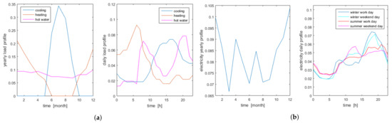
Figure 6.
Normalized thermal and electricity usage profiles. (a) Thermal usage. (b) Electricity usage.
On the other hand, as was mentioned previously, the electric load is separated into two classes: fixed and flexible. The flexible load, available for management trough DSM, is chosen to encompass the largest energy consumers. The nominal weekly appliance usage plan with appropriate timeframes for shifting is depicted in Table 1. A notable addition to the plan was made with the inclusion of an electric vehicle (EV) with its effect on DSM signified by [28]. As this load accounts for a total of 17,672 kWh in yearly electric energy consumption, or when not considering the EV, the remaining portion, attributed to appliances not listed as flexible (i.e., lighting, refrigeration, etc.), was chosen to equal and is distributed similarly as the thermal load using normalized usage profiles for electricity depicted in Figure 6b. In this case, four types of daily profiles are considered: winter work day, winter weekend day, summer work day, and summer weekend day and so repeating these segments appropriately results in a fixed electric demand time series as presented in the Figure 7. A thing to note is that both graphs from Figure 7 include daily and hourly noise in a similar fashion as is contained in popular microgrid software solutions like HOMER.

Table 1.
Flexible load weekly usage plan.

Figure 7.
Fixed year-long hourly electric demand. (a) Without STC and GSHP. (b) From STC and GSHP.
The constructed baseline, having in mind tariff information given in Section 4.2, equates to a nominal spending of for gas and for electricity totaling if considering a general use case where the thermal demand is met with gas. This number, inclusive of standing charges, will be used later on when discussing feasibility of selected configurations.
4.4. Renewable Technologies
To perform the operation optimization, the models from Appendix A need to be instantiated with real-word values corresponding to the selected use case site. First of all, data from TMY records [29] for the given location is obtained to be fed into the RES models for estimated production and demand calculations. Starting with the WT, a power curve is assumed after the manufacturer data for the Lely Aircon 10 turbine. The obtained power curve, normalized for one unit of power of installed capacity, is shown in Figure 8a. When the specified model is used to estimate the power production of the same normalized WT over the course of a year, including parameters given at the top of Table 2, the model gives the results depicted in Figure 8a. Moving on, using the PV parameters from Table 2 for the Suntech STP250S-20/Wd monocrystalline solar module, we may estimate the yearly production of the PV array per unit power considering the appropriate weather data for the use case location, as is presented in Figure 8b.
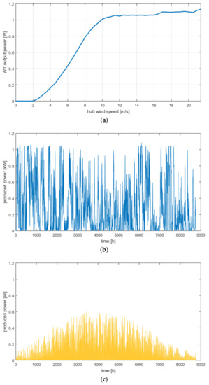
Figure 8.
RES generation. (a) WT curve. (b) WT generation. (c) PV generation.
Table 2.
Parameters for RET modeling.
Finally, the values required for STC and GSHP modeling are given in Table 2. When applying aforementioned TMY data in conjunction with this data to the appropriate models, having in mind the thermal demand profiles set in Section 4.3, Figure 7b is obtained showing the part of fixed electric demand required for running the GSHP, and thus, meeting the thermal demand of the system.
4.5. Objective Function Parameters
In accordance with the data given in Section 4.2, the tariff related parameters of the cost function are set to equal
Given the fact that out of the flexible appliances that were modeled, only the EV is set to be dispersible with maximum power draw deviations of per cent of its nominal value, and also having in mind that splitting its charging process into several sections probably does not impact the user’s comfort in a significant manner, was set for all appliances i and all time steps As for the CO emissions criteria, the carbon footprint values for energy sources were set to , and in accordance with the fuel mix data provided by ScottishPower [30] and median values that can be obtained from renewable production statistics.
4.6. Available Configurations
Since the multicriteria analysis is conceptualized as an exhaustive search over a preselected domain, that domain must be specified before the optimization is performed. Therefore, a set of renewable generators and storage options is formulated as depicted in Table 3. The pricing for the WT is loosely based on extrapolations of market data from EnergySavingTrust [31], the PV pricing can be found in a detailed statistical sheet compiled by BEIS [32] and BESS parameters are closely related to those that can be found in the technical documentation for the LG CHEM RESU [33] battery series and quotes by renewable technology resellers.
Table 3.
WT, PV, and BESS options.
The rest of the system is not considered within the sizing optimization process. This includes the installation for the GSHP system (construction work, piping, fittings, etc.), the pump and the STC. The pump and STC are considered to have an expected life span of 20 years while the GSHP installation generally lasts around 100 years before needing to be replaced. The initial acquisition costs are considered to be for the STC, for the GSHP installation and groundwork and for the pump given that a system is to be installed which is estimated to fulfill the thermal demand of the considered household. The associated yearly maintenance cost with running all of the aforementioned renewable technologies is set to 2% of initial acquisition cost.
5. Results
The operational optimization was performed using the CPLEX® Matlab Toolbox for all 100 selected configurations in both DSM off and on states with a time constraint of five minutes per configuration and was finished in about 10 hours. An illustrative example of an optimized operation of a modeled appliance is given in Figure 9a with an overview of all relevant energy assets for the same time frame presented in Figure 9b. The results in the space of the proposed criteria for all considered configurations are presented in Figure 10. The Pareto frontier formed by the set of nondominated solutions depicting the best compromise-free solution set is accented over the rest of the obtained results.
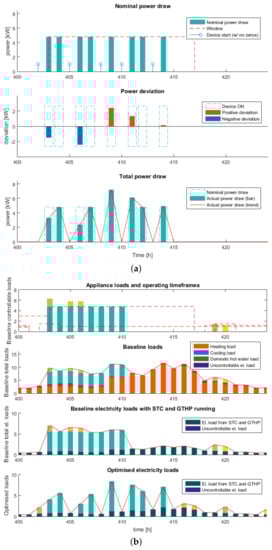
Figure 9.
Single appliance and total load optimization examples. (a) Example appliance (EV). (b) Total load.
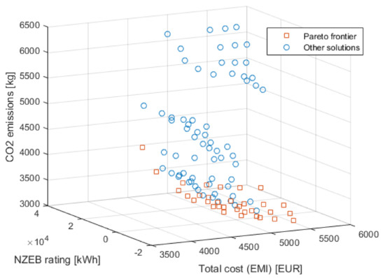
Figure 10.
Considered HRES configurations in criteria space.
However, given that the end result of the optimization process is considered to be only one, best solution, in the context of MCDMA ranking, the final outcome is highly dependent on the selected weights of each of the criteria that are imposed. Since each user will have different preferences, the decision space is practically infinite, however a couple of concrete examples are discussed to showcase the capabilities of the proposed planning strategy. Four different use cases will be presented to provide illustrative examples of how the optimum configuration changes in line with the criteria weight selection process. The first two will place a larger focus on monetary costs with the first one only considering them while the second introduces concerns for the supply and demand balance as well as for estimated environmental pollution. On the other hand, the third and fourth use case place a larger focus on the energy balance and emissions, respectively, while also including, but reduced, concern for monetary costs of running the system.
5.1. Total Cost as the Only Criterion
For the sake of simplicity, the first considered setup only focuses on minimizing the estimated total cost criterion through the appropriate set of weights
In the optimization process, the results were first obtained without employing DSM giving a midway baseline, and the five most cost-effective solutions are shown in Table 4. As can be clearly seen, implementing only raw renewable sources without any additional optimization, in this case, does not yield significant monetary savings when compared with the gas and electricity no-renewable baseline, with the best option well below 3%. The third best, and all following combinations without DSM are not even profitable, with the fifth one costing over 3% more than the original baseline.
Table 4.
List of five best configurations when solely focusing on cost with DSM turned off.
However, when DSM is turned on, the order of best solutions, depicted in Table 5, changes somewhat, with the best case scenario (using a WT) returning savings slightly above 10% allowing the investment to be considered well worthwhile. A thing to note is that no PV production is included in this best-case scenario which should not be surprising since the considered site does not receive a significant enough amount of sunlight for PV to be cost-effective. However, the absence of BESS in the optimal solution is of significantly greater interest since the obtained result can be considered to show that an efficient implementation of a DSM program can lower the requirement for expensive and potentially environmentally unfriendly solutions like lithium-ion batteries that are commonly used for storing off-peak electric energy. Slightly less cost-effective then the best solution is the combination with the WT, with the fifth best solution finally including the smallest considered PV panel array, and the sixth including a battery with the originally selected WT.
Table 5.
List of six best configurations when solely focusing on cost with DSM turned on.
5.2. Total Cost as the Primary Criterion
On the other hand, cost need not be considered as the sole criterion when selecting the optimal configuration. Choosing different weights allows for the user to specify what criteria he deems relevant, and thus, the software adjusts the optimal configuration rankings. One such mixed case where cost is still the primary focus, but the other two environmental criteria are also taken into consideration can be defined by selecting appropriate weights to equal
After ranking the optimally preforming configurations in accordance with the above-mentioned weights, the best combination and a list of best alternatives is obtained and presented in Table 6. The results show that although monetary savings are still the prevalent considered parameter, this type of selection slightly favors large renewable sources due to the associated decrease in discrepancy between the spent and produced amount of energy and the equivalent amount of CO emitted.
Table 6.
List of five best configurations when primarily focusing on cost with DSM turned on.
5.3. NZEB Rating as the Primary Criterion
Also, environmental criteria can be accented if the project is such that the ecological impact is more of a priority. One possible weight selection that would accomplish this could be
Adequate ranking resulted in the list presented in Table 7. Since the monetary aspect is no longer the primary concern, the best selected solutions are generally not profitable when compared to baseline costs. However, they are significantly more ecologically friendly, with all of them generating significantly more energy on-site than is being consumed and CO being cut by about 40 to 50% when compared with that of the configuration without WT, PV, and BESS for all the presented alternatives.
Table 7.
List of five best configurations when primarily focusing on NZEB rating with DSM turned on.
5.4. CO2 Emissions as the Primary Criterion
Finally, amongst environmentally friendly use cases, the main stressed criterion could be emissions, as is accomplished by
The resulting ranking in this case is presented in Table 8. As was expected, the best solutions are, just like in the aforementioned case, not the most profitable, but offer significant environmental features. Nonzero BESS units now appear in all of the selected configurations because of the need to minimize the emissions trough using locally produced electricity as opposed to grid imports.
Table 8.
List of five best configurations when primarily focusing on emissions with DSM turned on.
5.5. Use Case without Incentives
In the end, for reference purposes, a use case is assumed where the various incentives that were previously considered are set to zero. This use case is obtained by specifying
and also setting the RHI incentive to zero for both STC and GSHP. Since the process of energy trading on the wholesale market would certainly include multiple middlemen that would reduce the benefit that the user exporting energy can make use of, this use case assumes arguably generous renewable energy export prices at the same value as is the price of importing electricity from the grid. However, when the operational optimization is performed for configurations that include batteries with capacities of 0 and , PV arrays with capacities of 0 and and all wind turbine configurations with nonzero capacities and the resulting results are analyzed with a sole focus on minimizing costs, the results from Table 9 are obtained. Results show that the event is the best-case scenario without incentives is more than 35% more expensive than the nonrenewable baseline, thus reaffirming the conclusion that the renewable installation project in the discussed case continues to highly depend on the existences of some of the mentioned incentive programs to be cost-effective.
Table 9.
List of five best configurations when optimizing solely for costs without any incentives and with DSM turned on.
6. Conclusions
The methodology presented in this paper details a comprehensive optimization process with a proposed linear programming-based model for operational optimization and a multicriteria ranking system for sizing optimization. To illustrate the capabilities of that process, a use case is assumed and the optimizer was employed to prove that the investment in renewable sources can be cost-effective when adequate appliance management techniques are used, resulting in savings just over 10% when only costs are considered as a primary criterion, in line with findings that could be found in the discussed related literature. The algorithm also manages to yield configurations with significant environmental impact improvements when compared to a nonrenewable baseline when the focus is shifted from costs to ecological factors. Also, in some of the selected cases, the obtained optimal solutions show an absence of storage solutions, which shows that DSM methods can be employed to reduce the negative environmental impact of costly chemical-based batteries that are often associated with HRES systems. Although the selected demonstration site was not comprehensive in terms of utilization of all energy sources featured by the Energy Hub methodology, additional sources can effortlessly be integrated into a similar analysis should the use case differ from the presented one.
A crucial aspect that should be considered for the demonstrated energy efficiency improvements to be realized in an arbitrary real-world setting are potential policy and legislative limitations. With different governments offering different terms for energy prosumers, local regulations should be, as was the done in the demonstrated use case, carefully analyzed when approaching both the planning and operation stages of the project. However, results presented in this paper and related publications can hopefully serve as a positive use case and aid in policy adjustments for the benefits of energy end users, energy producers, and grid operators.
Further research in this field is planned to include the implementation of more complex stochastic models into the production and load profiles as well as nominal appliance usage to more accurately model day-to-day variances in user demand. Furthermore, the demand-side management aspect can be extended by also including demand response events that would facilitate load increases or decreases during predefined periods of time. Also, the sizing optimization paradigm could be extended to all sustainable sources like the heat pumps and thermal storage units. However, this extension may involve more detailed numerical models that would dynamically assess operation of the mentioned components to ensure long-term efficiency. Finally, the effects of different time step lengths and the introduction of different new criteria should also be analyzed to provide a holistic view of solutions that can be obtained in the desired decision space.
Author Contributions
Conceptualization, M.B. and N.T.; methodology, M.B.; software, M.J.; validation, M.J., M.B.; formal analysis, M.B. and N.T.; investigation, M.J.; resources, M.B. and N.T.; data curation, M.J.; writing—original draft preparation, M.J.; writing—review and editing, M.B. and N.T.; visualization, M.J.; supervision, M.B. and N.T.; project administration, N.T.; funding acquisition, M.B. and N.T. All authors have read and agreed to the published version of the manuscript.
Funding
The research presented in this paper is partly financed by the European Union (H2020 SINERGY project, Grant Agreement No.: 952140) and the Ministry of Education, Science and Technological Development and the Science Fund of the Republic of Serbia (AI-ARTEMIS project, #6527051).
Conflicts of Interest
The authors declare no conflict of interest.
Appendix A. Modeling Renewable Technologies
Including renewable sources like the WT, PV panels as well as heating and cooling solutions like the STC and GSHP into the system requires proper modeling of their operation to evaluate the model’s performances. Therefore, this section is set to outline the models used for describing RES behavior.
Appendix A.1. Wind Turbine
Following the methodology depicted in [34], the power of a WT is generally calculated based upon a power curve which outputs the generated power when the wind speed at the hub of the generator is in test conditions. However, the actual generated power values do not exactly match the ones from the test power curve because they need to be scaled by the installed capacity and adjusted for the difference in air density. This effect is modeled by
where the ratio between the air density at the hub and in test conditions (at sea level and 15 C temperature) can be calculated as
Wind speed measurements at heights equivalent to those of turbine hubs are usually not readily available, and therefore must be estimated. According to [35], a logarithmic profile can be used to estimate the wind speed at the hub based on the speed at the anemometer by using
Appendix A.2. Photovoltaic Panels
Modeling the output of a photovoltaic panel is somewhat more complex that modeling the WT since the output of the panel depends on several different factors. Namely, according to [36,37], it can be modeled as
Irradiance can be calculated as
based on individual components and where
The angle determining the slope of the surface with representing a horizontal panel and a vertical panel. Having in mind [38], the components of solar irradiation required for applying (A4) can either be obtained from a meteorological database or estimated using appropriated models that are beyond the scope of this paper. Furthermore, the cell temperature is attained from
where
The maximum power point efficiency is calculated as
Appendix A.3. Solar Thermal Collector
The STC is modeled as a passive system (without a heat pump) based on [37,39] with two major components: the collector that extracts heat from the environment and the tank which stores that heat for later use. The temperature of the water in the tank can be calculated as
The tank naturally losses heat as is expressed by
Since this model is created for simulations utilizing a sample period equal to one hour, h is assumed when modeling STC processes with data for smaller sample periods available through interpolation. The heat produced by the collector can be obtained with
This formula is obtained as a nonlinear fit with experimental data where A is the amount of times that the area of the collector is greater than used in the original experiment and parameter values , and are taken from the original experiment. If the produced value is negative, the collector is detached as not to further reduce the amount of energy stored in the tank. Otherwise, the additional energy is injected into the tank, and so the available amount of heat can be expressed as
However, since the user’s demand at the considered time step is be subtracted, but may not be sufficient to meet all of the thermal needs. Thus, it is stated that the amount stored in the tank at the start of the next time step is
where
If the stored heat is limited by (A14) to the user’s demand was not fully met, and the unmet heat
is passed on to an auxiliary heating system whose role is played by the GSHP in the considered configuration.
Appendix A.4. Ground Source Heat Pump
The basic premise of the system by which the GSHP operates is utilizing the constant nature of soil temperature beneath and around the considered property. Following the bin method outlined in [40], the ground temperature is modeled as
where
Following this, the minimum and maximum ground temperatures are determined as
Even though the minimum and maximum temperature of water exiting the ground heat exchanger is directly influenced by these values, because of practical constraints, it is limited between
Using linear interpolation, the temperature of water at the entrance of the heat pump fed by a closed-loop ground exchanger can be determined as
where . A capacity multiplier forces the system to meet either the cooling demand with
with the appropriate cooling/heating capacity and COP of the GSHP being
Appropriate values for parameters k and used to fit these expressions are summarized in Table A1. Finally, having in mind that the amount of thermal energy that can be obtained by this system is limited by the designed power, and thus, may only be less than we set the consumed amount of electric energy to
where in the latter case auxiliary thermal sources must be used to fulfill the remaining part of the demand.
Table A1.
Quadratic polynomial coefficients.
Table A1.
Quadratic polynomial coefficients.
| Coefficients | Cooling | Heating | |
|---|---|---|---|
| COP | |||
| Capacity | |||
Appendix B. Nomenclature
Appendix B.1. Proposed Planning Methodology
| i-th alternative in the MCDMA | |
| k-th criterion out of q for | |
| pair-wise comparison value for criterion | |
| preference degree function | |
| preference function | |
| , | lower and upper preference boundaries |
| weight associated with criterion | |
| , , | positive, negative and net preference flow |
| wind turbine | |
| nominal power-wind speed WT power curve | |
| rated power (power capacity) of the WT system | |
| capacity and air density adjusted power-wind speed WT power curve | |
| , | air density at site and at test conditions |
| B | laps rate |
| standard temperature | |
| g | gravitational acceleration |
| R | universal gas constant divided by the molar mass of air |
| WT hub height above sea level | |
| anemometer and WT hub height above ground | |
| wind speed at anemometer and WT hub height | |
| surface roughness level | |
| photovoltaic | |
| instantaneous power generated by the PV system | |
| rated power (power capacity) of the PV system | |
| derating factor of the PV system | |
| solar irradiance incident on the PV array averaged at the current timestamp | |
| temperature coefficient of power | |
| PV cell temperature | |
| (at) standard test conditions | |
| , G | diffuse, beam and global horizontal irradiation |
| anisotropy index | |
| ratio between beam radiation on a tilted and horizontal surface | |
| f | horizontal brightening factor |
| PV surface slope | |
| ground reflectance (albedo) | |
| ambient temperature | |
| (at) nominal operating cell temperature | |
| maximum power point efficiency | |
| surface area of the PV array | |
| a | solar absorbance of the PV array cover |
| solar transmittance of the PV array cover | |
| solat thermal collector | |
| available amount of heat in the tank and lost amount of heat | |
| water temperature in the tank and ambient temperature | |
| m | mass of water in the tank |
| c | specific heat capacity of water |
| storage heat loss coefficient per unit of volume | |
| sample rate | |
| produced amount of heat and available amount of heat in the tank | |
| ground source heat pump | |
| ground temperature | |
| mean annual soil temperature | |
| annual surface temperature amplitude | |
| soil depth | |
| soil thermal diffusivity | |
| k | soil thermal conductivity |
| soil density | |
| soil specific heat | |
| t | day of the year |
| entering water temperature | |
| cooling/heating averaged design temperature | |
| binned ambient temperature | |
| capacity multiplier | |
| cooling/heating demand | |
| , | instantaneous coefficient of performance (COP) and at baseline |
| maximum design power | |
| electric energy consumed by GSHP |
Appendix B.2. Mathematical model
| input (imported) power | |
| input and output power to and from the converters | |
| power flow to/from the storage at the input and output stage | |
| L | loads |
| output power to loads | |
| exported power | |
| charge/discharge rate for storage at the input and output stages | |
| available energy (state of charge, SOC) for storage at the input and output stages | |
| y, z | device on/off and device start indicators |
| positive and negative power deviations | |
| indicators for positive and negative power deviations | |
| input stage energy storage conversion matrices | |
| input and output transformation matrices | |
| C | energy conversion matrix |
| , | export energy restriction matrices |
| output stage energy storage conversion matrices | |
| , | i-th appliance’s instantaneous and nominal power draw |
| i-th appliance’s n-th activation window indicator and length | |
| maximum absolute positive and negative power deviations | |
| power produced from renewable sources | |
| SOC capaciti limits at input and output stages | |
| cost, dispersion and mixed criterion | |
| , , | energy import and export prices and standing charge |
| i-th appliance dispersion penalization factor | |
| equated monthly installments and maintenance costs | |
| estimated lifetime in years for i-th device | |
| monthly discount rate | |
| initial acquisition cost for i-th device | |
| cost, net-zero energy building (NZEB) and CO2 emission criterion | |
| carbon footprint values for WT, PV and grid imported energy |
Appendix B.3. Use Case
| baseline thermal energy requirements for heating and domestic hot water (DHW) |
References
- European Commission. Renewable Energy | Energy. 2019. Available online: ec.europa.eu (accessed on 27 September 2021).
- nzeb | European Commission. 2016. Available online: ec.europa.eu (accessed on 27 September 2021).
- Sinha, S.; Chandel, S.S. Review of software tools for hybrid renewable energy systems. Renew. Sustain. Energy Rev. 2014, 32, 192–205. [Google Scholar] [CrossRef]
- Xu, L.; Ruan, X.; Mao, C.; Zhang, B.; Luo, Y. An Improved Optimal Sizing Method for Wind-Solar-Battery Hybrid Power System. IEEE Trans. Sustain. Energy 2013, 4, 774–785. [Google Scholar] [CrossRef]
- Alsayed, M.; Cacciato, M.; Scarcella, G.; Scelba, G. Multicriteria Optimal Sizing of Photovoltaic-Wind Turbine Grid Connected Systems. IEEE Trans. Energy Convers. 2013, 28, 370–379. [Google Scholar] [CrossRef]
- Akram, U.; Khalid, M.; Shafiq, S. Optimal sizing of a wind/solar/battery hybrid grid-connected microgrid system. IET Renew. Power Gener. 2018, 12, 72–80. [Google Scholar] [CrossRef]
- Scalfati, A.; Iannuzzi, D.; Fantauzzi, M.; Roscia, M. Optimal sizing of distributed energy resources in smart microgrids: A mixed integer linear programming formulation. In Proceedings of the 2017 IEEE 6th International Conference on Renewable Energy Research and Applications (ICRERA), San Diego, CA, USA, 5–8 November 2017; pp. 568–573. [Google Scholar] [CrossRef]
- Husein, M.; Chung, I.Y. Optimal design and financial feasibility of a university campus microgrid considering renewable energy incentives. Appl. Energy 2018, 225, 273–289. [Google Scholar] [CrossRef]
- Wang, X.; Palazoglu, A.; El-Farra, N.H. Operational optimization and demand response of hybrid renewable energy systems. Appl. Energy 2015, 143, 324–335. [Google Scholar] [CrossRef]
- Mazzeo, D.; Baglivo, C.; Matera, N.; Congedo, P.M.; Oliveti, G. A novel energy-economic-environmental multicriteria decision-making in the optimization of a hybrid renewable system. Sustain. Cities Soc. 2019, 52, 101780. [Google Scholar] [CrossRef]
- Hernández, J.C.; Sanchez-Sutil, F.; Muñoz-Rodríguez, F.J.; Baier, C.R. Optimal sizing and management strategy for PV household-prosumers with self-consumption/sufficiency enhancement and provision of frequency containment reserve. Appl. Energy 2020, 277, 115529. [Google Scholar] [CrossRef]
- Achiluzzi, E.; Kobikrishna, K.; Sivabalan, A.; Sabillon, C.; Venkatesh, B. Optimal Asset Planning for Prosumers Considering Energy Storage and Photovoltaic (PV) Units: A Stochastic Approach. Energies 2020, 13, 1813. [Google Scholar] [CrossRef] [Green Version]
- Barbato, A.; Capone, A. Optimization Models and Methods for Demand-Side Management of Residential Users: A Survey. Energies 2014, 7, 5787–5824. [Google Scholar] [CrossRef]
- Lokeshgupta, B.; Sivasubramani, S. Multi-objective home energy management with battery energy storage systems. Sustain. Cities Soc. 2019, 47, 101458. [Google Scholar] [CrossRef]
- Clastres, C.; Ha Pham, T.T.; Wurtz, F.; Bacha, S. Ancillary services and optimal household energy management with photovoltaic production. Energy 2010, 35, 55–64. [Google Scholar] [CrossRef] [Green Version]
- Barbato, A.; Capone, A.; Carello, G.; Delfanti, M.; Merlo, M.; Zaminga, A. House energy demand optimization in single and multi-user scenarios. In Proceedings of the 2011 IEEE International Conference on Smart Grid Communications (SmartGridComm), Brussels, Belgium, 17–20 October 2011; pp. 345–350. [Google Scholar] [CrossRef]
- Bradac, Z.; Kaczmarczyk, V.; Fiedler, P. Optimal Scheduling of Domestic Appliances via MILP. Energies 2015, 8, 217–232. [Google Scholar] [CrossRef]
- Atia, R.; Yamada, N. Sizing and Analysis of Renewable Energy and Battery Systems in Residential Microgrids. IEEE Trans. Smart Grid 2016, 7, 1204–1213. [Google Scholar] [CrossRef]
- Batić, M.; Tomašević, N.; Beccuti, G.; Demiray, T.; Vraneš, S. Combined energy hub optimization and demand side management for buildings. Energy Build. 2016, 127, 229–241. [Google Scholar] [CrossRef]
- Favre-Perrod, P. A vision of future energy networks. In Proceedings of the 2005 IEEE Power Engineering Society Inaugural Conference and Exposition in Africa, Durban, South Africa, 11–15 July 2005; pp. 13–17. [Google Scholar] [CrossRef]
- Siksnelyte, I.; Zavadskas, E.K.; Streimikiene, D.; Sharma, D. An Overview of Multi-Criteria Decision-Making Methods in Dealing with Sustainable Energy Development Issues. Energies 2018, 11, 2754. [Google Scholar] [CrossRef] [Green Version]
- Brans, J.P.; Vincke, P. Note—A Preference Ranking Organisation Method. Manag. Sci. 1985, 31, 647–656. [Google Scholar] [CrossRef] [Green Version]
- Zappa, W.; Junginger, M.; van den Broek, M. Is a 100% renewable European power system feasible by 2050? Appl. Energy 2019, 233–234, 1027–1050. [Google Scholar] [CrossRef]
- Suh, H.S.; Kim, D.D. Energy performance assessment towards nearly zero energy community buildings in South Korea. Sustain. Cities Soc. 2019, 44, 488–498. [Google Scholar] [CrossRef]
- Online Fixed Saver | ScottishPower. Available online: scottishpower.co.uk (accessed on 15 August 2019).
- Public Reports and Data: Domestic RHI | OFGEM. Available online: ofgem.gov.uk (accessed on 27 September 2021).
- Energy Consumption in the UK | UK Government. Available online: gov.uk (accessed on 27 September 2021).
- Mesarić, P.; Krajcar, S. Home demand side management integrated with electric vehicles and renewable energy sources. Energy Build. 2015, 108, 1–9. [Google Scholar] [CrossRef]
- Typical Metheorlogical Year (TMY) | European Commission. Available online: ec.europa.eu (accessed on 27 September 2021).
- Fuel Mix Information | ScottishPower. Available online: scottishpower.co.uk (accessed on 27 September 2021).
- Wind turbines | EnergySavingTrust. Available online: energysavingtrust.org.uk (accessed on 27 September 2021).
- Solar Photovoltaic (PV) Cost Data | UK Government. Available online: gov.uk (accessed on 27 September 2021).
- LG Chem Catalog Global 2018 | LG. 2018. Available online: m.lgchem.com (accessed on 27 September 2021).
- Deshmukh, M.K.; Deshmukh, S.S. Modeling of hybrid renewable energy systems. Renew. Sustain. Energy Rev. 2008, 12, 235–249. [Google Scholar] [CrossRef]
- Holmes, J. Wind Loading of Structures, 3rd ed.; CRC Press: Boca Raton, FL, USA, 2017. [Google Scholar]
- Patel, M. Wind and Solar Power Systems: Design, Analysis, and Operation, 2nd ed.; CRC Press: Boca Raton, FL, USA, 2005. [Google Scholar]
- Duffie, J.; Beckman, W. Solar Engineering of Thermal Processes, 4th ed.; John Wiley & Sons: Hoboken, NJ, USA, 2013. [Google Scholar]
- Erbs, D.G.; Klein, S.A.; Duffie, J.A. Estimation of the diffuse radiation fraction for hourly, daily and monthly-average global radiation. Sol. Energy 1982, 28, 293–302. [Google Scholar] [CrossRef]
- Elasfouri, A.S.; Hawas, M.M. A simplified model for simulating solar thermal systems. Energy Convers. Manag. 1987, 27, 1–10. [Google Scholar] [CrossRef]
- Canada Natural Resources, Canada Energy Sector. Clean Energy Project Analysis, RETScreen Engineering & Cases Textbook, 3rd ed.; Natural Resources Canada: Nepean, ON, Canada, 2005. [Google Scholar]
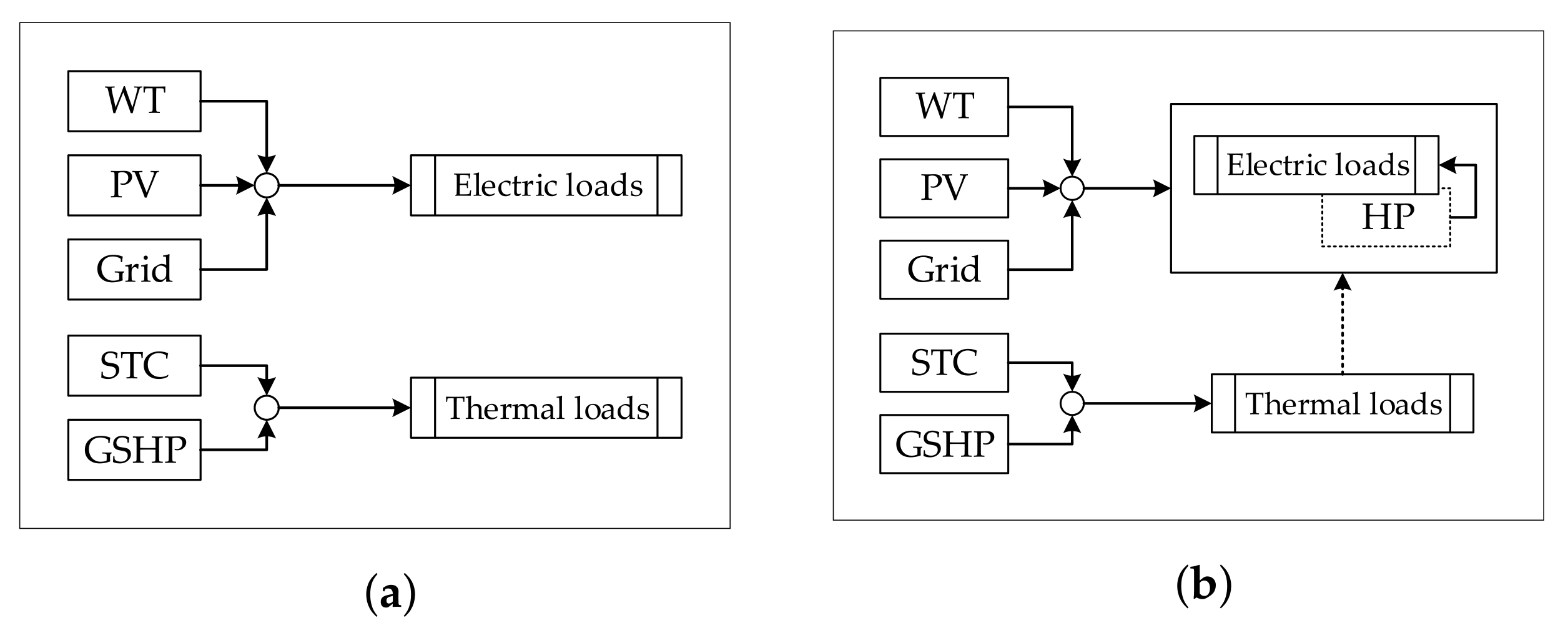
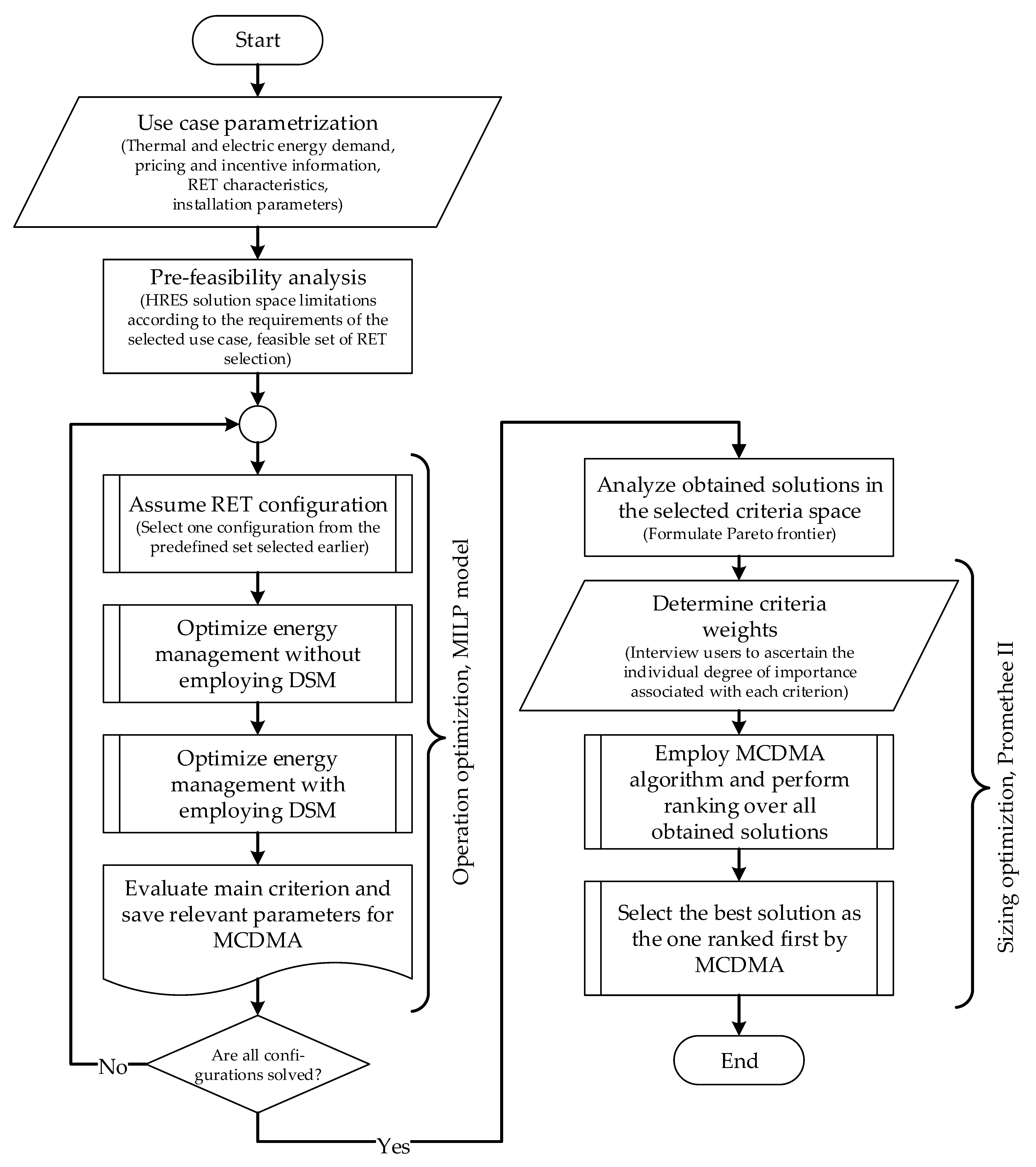

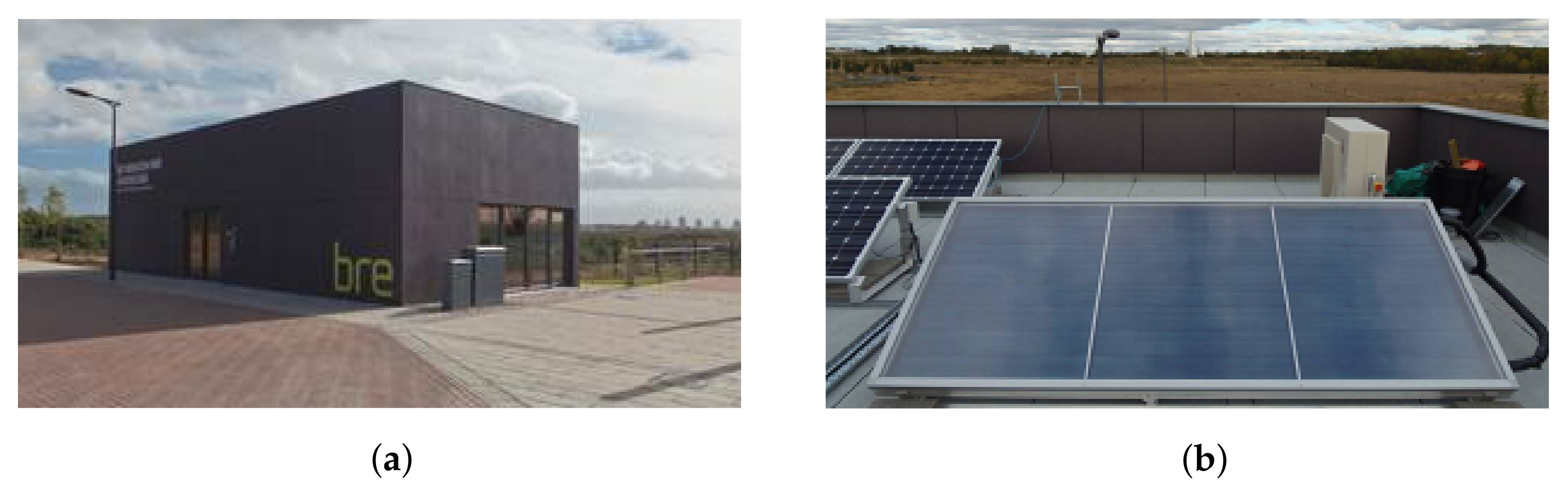
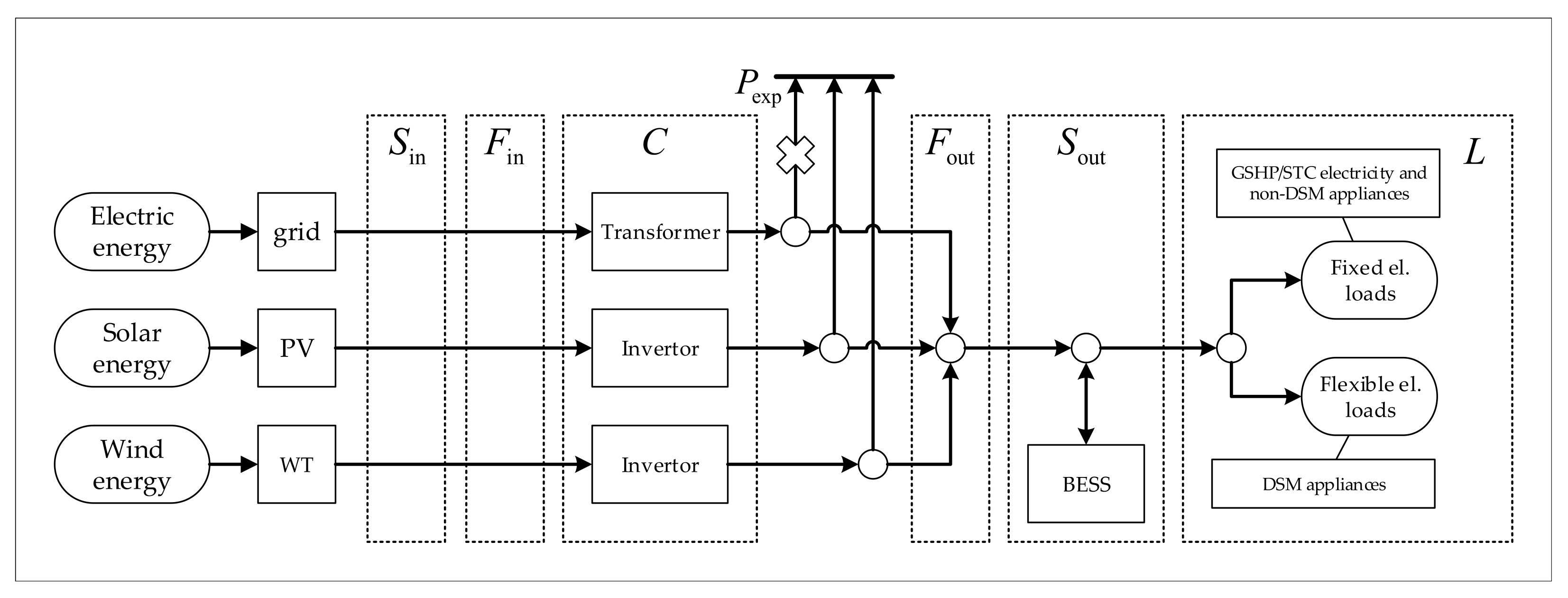
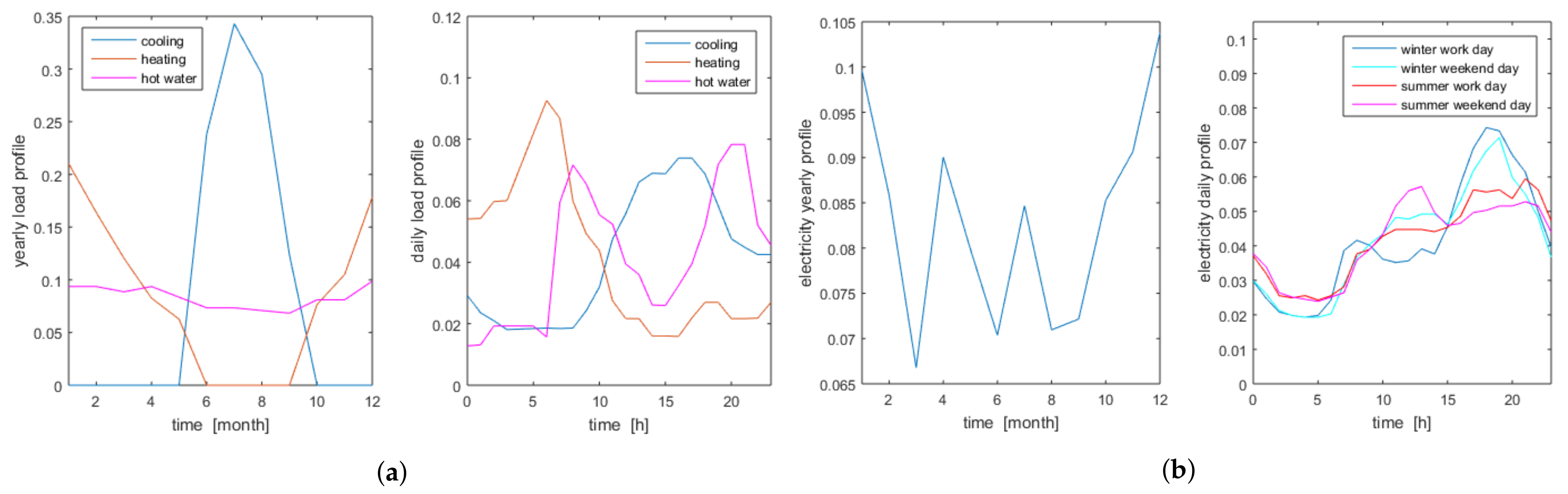
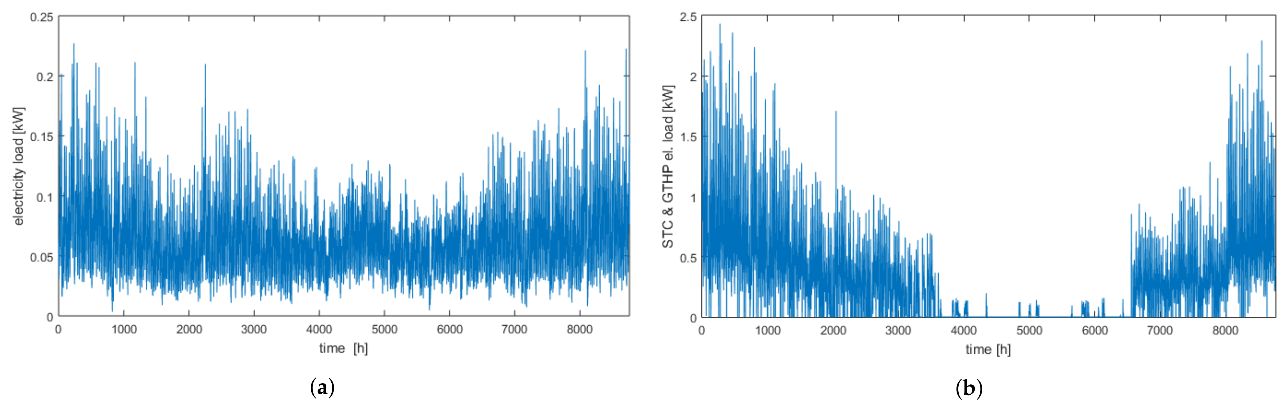


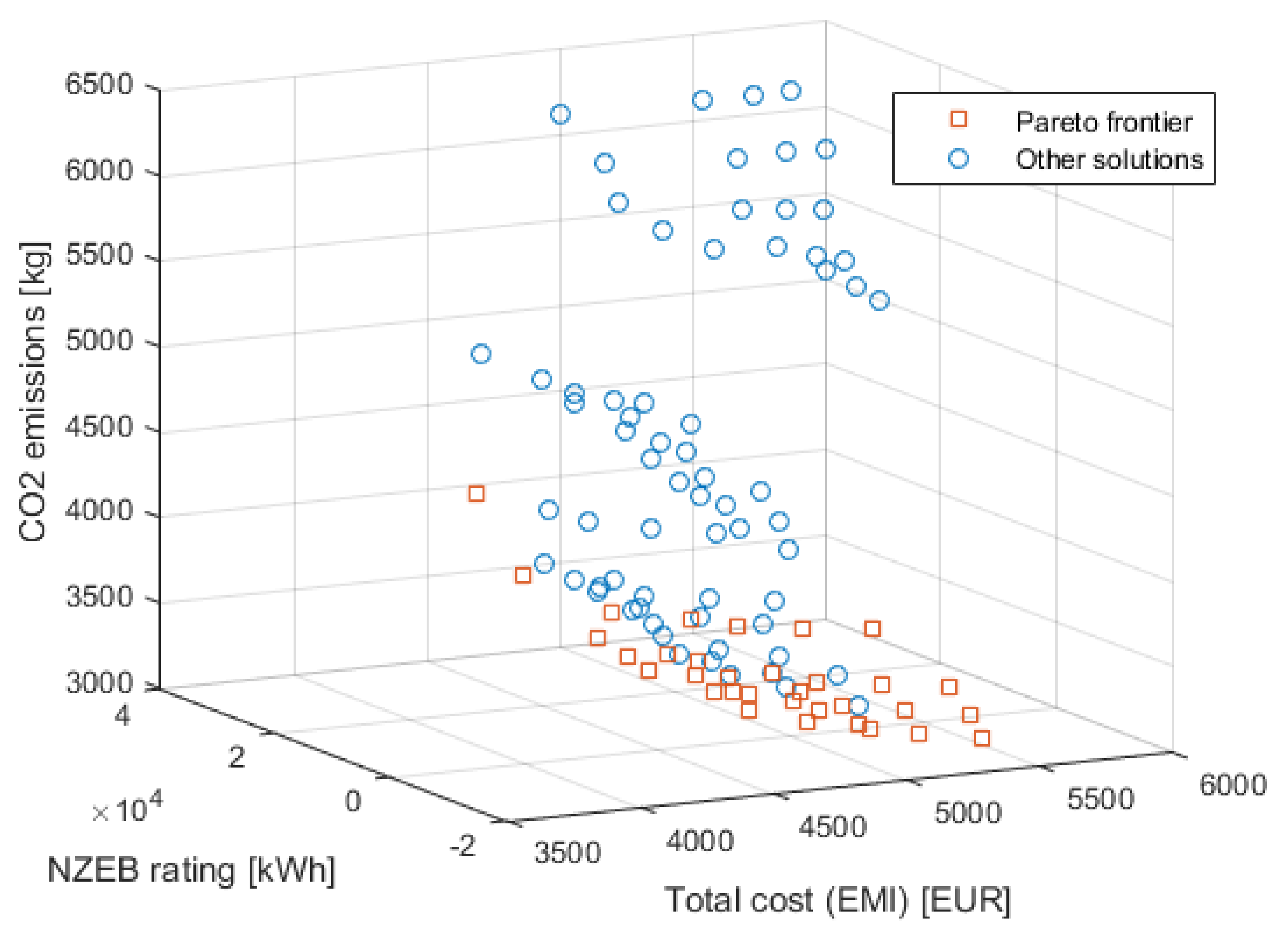
Publisher’s Note: MDPI stays neutral with regard to jurisdictional claims in published maps and institutional affiliations. |
© 2021 by the authors. Licensee MDPI, Basel, Switzerland. This article is an open access article distributed under the terms and conditions of the Creative Commons Attribution (CC BY) license (https://creativecommons.org/licenses/by/4.0/).