Abstract
Short-term load forecasting predetermines how power systems operate because electricity production needs to sustain demand at all times and costs. Most load forecasts for the non-residential consumers are empirically done either by a customer’s employee or supplier personnel based on experience and historical data, which is frequently not consistent. Our objective is to develop viable and market-oriented machine learning models for short-term forecasting for non-residential consumers. Multiple algorithms were implemented and compared to identify the best model for a cluster of industrial and commercial consumers. The article concludes that the sliding window approach for supervised learning with recurrent neural networks can learn short and long-term dependencies in time series. The best method implemented for the 24 h forecast is a Gated Recurrent Unit (GRU) applied for aggregated loads over three months of testing data resulted in 5.28% MAPE and minimized the cost with 5326.17 € compared with the second-best method LSTM. We propose a new model to evaluate the gap between evaluation metrics and the financial impact of forecast errors in the power market environment. The model simulates bidding on the power market based on the 24 h forecast and using the Romanian day-ahead market and balancing prices through the testing dataset.
1. Introduction
The risks of climate change drive the acceleration of energy transition from fossil fuels to renewables, exposing energy vulnerability as debated by [1]. The social, economic, and environmental aspects need careful attention regarding the development of clean energies [2]. The European Union has bold plans to become, by 2050, the world’s first climate-neutral continent as decided through the New Green Deal [3] by using 100% renewable electricity. All these ambitious sustainable plans face limitations in transmission capabilities [4] and demand flexibility, Ref. [5] outlines scenarios where renewable energy sources face increased curtailment from operation by 2050.
1.1. Context and Importance of Load Forecasting
Reliable electricity load forecasting can offer great value to the above plans, and machine learning (ML) could revolutionize smart grids operations dealing with large amounts of data [6,7,8]. It is a field intensively researched because of the financial repercussions and the importance of optimally balancing the power grid [9]. The authors of [10] showcase the importance of energy bill costs for electricity-consuming industries to remain competitive in global markets. The present article focuses on short term load forecasting for industrial and commercial consumers and offers arguments for the demand side to engage in more active collaboration in the power market.
The novelty of our article is a new method for the evaluation of the short-term load forecasting results and a framework suitable for energy suppliers that need to manage a diverse portfolio. The industry needs algorithms capable of automating the process of forecasting. Another contribution of the article is to compare the aggregate and individual forecasts by applying the same algorithms and methodologies to evaluate results. The machine learning algorithms use data from a cluster of industrial and commercial loads.
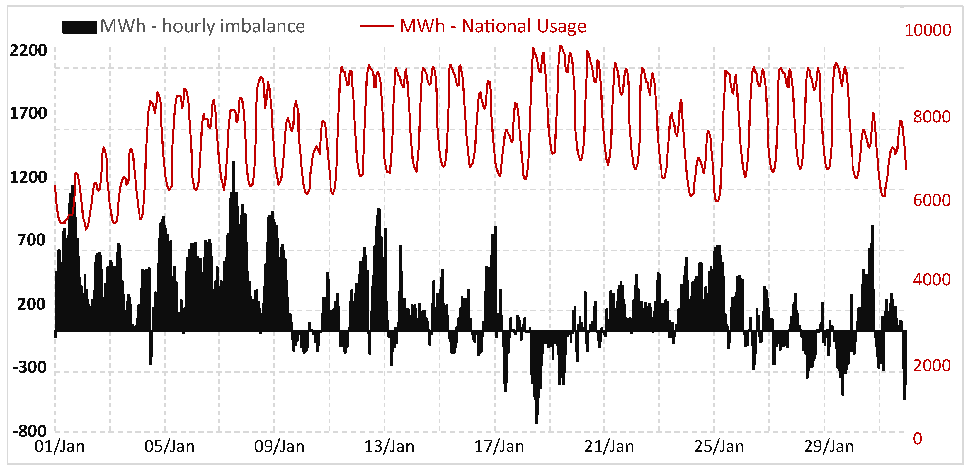
To highlight the importance of power grid imbalances we present data for the Romanian transmission system operator (TSO) in Figure 1. Load forecasting accuracy impacts the entire power market participants. Forecasting errors directly influence the costs generated by grid imbalances.
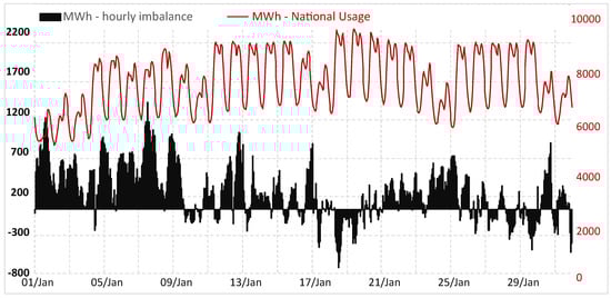
Figure 1.
Romanian national hourly electricity imbalances.
In Figure 1, the imbalance represents the difference between forecast values notified on the balancing market (BM) and real measured values. The total hourly electricity imbalance in January 2021 represents a value of 4%(219.7 GWh) in the overall national consumption (5586.4 GWh). Data are available at the market operator website OPCOM (accessed on 12 September 2021).
The first section of the article discusses the importance of electricity load forecasting and the current state of knowledge for forecasting algorithms. Section 2 presents the software resources and the available dataset by providing information for electricity consumers. The section details the algorithms and the methodology for forecasting. Two approaches for forecasting are implemented: aggregated and individual forecasts according to the cluster of consumers. The reason for these approaches is the effort to simulate the operation of an electricity supplier active on the power market according to a complex portfolio. In Section 3, the forecast results are presented together with a new method for assessing the impact of consumption forecasts on the energy market. The new evaluation method assesses the forecasts obtained from a practical point of view. In the last sections, the authors discuss the general conclusions and discussions.
1.2. Literature Review: Traditional Approach
Simple statistical methods such as moving average (MA) models can be effective, a 7-day moving average on regional level consumption was applied by [11] and obtained a 30.55 MW mean error and MAPE (mean absolute percentage error) of 3.84%. Exponential smoothing (ES) is a commonly used technique where a smoothed time series is generated by assigning variable weights to the observed data point, depending on how old the data are. Proposed by Holt (1957) and studied by Winters (1960) [12], the Holt–Winters (H–W) method consists of three smoothing equations for level, trend, and seasonality. A simple approach is to implement naive methods to build a valid benchmark for load forecasting in order to have a comparison standpoint. The authors of [13] implemented Holt–Winters Exponential Smoothing in comparison with two naive benchmark methods showing the inferiority of the latter. Various equations [14] can be used to implement such algorithms, for example, the average method.
Another widely implemented method is ARIMA (autoregressive integrated moving average), a statistical method that interprets time series data to predict future values based on past correlations. ARIMA model was proposed by Box and Jenkins [15] and has three components: autoregressive, integrated, and the moving average of the dataset.
1.3. Literature Review: Machine Learning
Various neural networks (NN) studied by [16] point to long short-term memory (LSTM) as the best method with MAPE of 1.55%. In this article, a similar approach was implemented for supervised learning like the authors present in [17]. Extensive analysis of literature by [18] reviewed methods of load forecasting based on 126 research articles of STFL. The authors of [19] present the superiority of deep learning (DL) in comparison with the traditional Sarimax algorithm, the conclusion reached by this article as well. Support vector machines (SVR) and artificial neural networks (ANN) applied by [20] for buildings obtained an average error rate of 3.46–10%, and ANN performed better than SVR.
In the present article, the novelty characteristic is the implementation of machine learning algorithms for a cluster of industrial and commercial loads, adapted for the requirements of the Romanian power market, which is the second volatile market in the European Union according to [21]. The significant novelty aspect introduced by the article is the performance evaluation method, which compares the algorithms based on the power market impact. In the literature, the authors refer to well-known metrics such as SMAPE (symmetric mean absolute percentage error), MAPE (mean absolute percentage error), RMSE (root mean squared error), or MAE (mean absolute error). The authors of [22] rank accuracy metrics for forecasting as follows: MSE > SMAPE = MAPE > MAE > RMSE > > R. In this article, the evaluation for the test dataset simulates power market exposure based on the forecast obtained by all the algorithms implemented. Electricity suppliers and private entities could be better stimulated to offer greater importance for energy usage and forecasting if provided with a cost-benefit analysis rather than a percentage value.
The ML algorithms implemented in the article used as inputs the past two weeks of hourly consumption data and exogenous variables for the supervised training of the NN according to the methodology proposed by [23]. In [24], the authors propose a similar approach to the one presented in this article but on buildings’ electricity consumption. The article concludes that forecasting on building-level data, rather than aggregating the results to predict the aggregated load produces more accurate forecasts, results that differ from our analysis on industrial and commercial loads. RNN algorithms and MLP was implemented on a group of buildings for 24 h ahead forecasting by using machine learning, and the best results are achieved by Random Forest in comparison with ML, LSTM, and KNN (K-Nearest Neighbor). An online adaptive RNN was implemented in [25] and was compared to RNN and MLP, the 3 year dataset was split into 70% and 30%. In this article, the dataset split is 80% training and 20% testing, because the load curves for all the consumers in the cluster are available for one year. Additionally, the purpose of this article is to research the best forecasting technique from a practical perspective, the reason for which the learning does not keep track of updated load curves. The consumers analyzed do not have advanced smart metering and the data is obtained at the end of the day from the DSO (distribution system operator), this being a major setback for the Romanian electricity sector as pointed out by [26]. In [27] a hybrid algorithm based on SVM (support vector machines), RF (random forest), and LSTM is proposed on aggregated load curves as a viable solution but uses only 1.6% of the data to test the accuracy of forecasting. For industrial load authors, authors [28] propose a combination of RNN with 1D CNN (Convolution neural network) and obtain similar results with the LSTM-CNN method implemented in this article. The forecast horizon is for the next day, 48-time points at 30 min intervals, the train and test split is 75% and 25%. Electricity price is used by the authors of [29] as input in a GRU network for forecasting electricity consumption at the utility level. In our analysis, because of the types of tariffs, this is not applicable. Due to the latest development in energy prices, this approach could become efficient for short to medium-term forecasting. According to [30], Romanian has one of the highest prices for balancing, and a significant number of participants. In 2019 the price for the deficit was 124 €/MWh and 2 €/MWh for surplus.
2. Materials and Methods
2.1. Case Study Data Analysis—Hourly Industrial and Commercial Demand
The forecasting methods implemented in this article are applied to hourly data from a group of five non-residential consumers for an entire year (2019). Industrial energy use allows factories to exploit resources in order to produce goods and use is different from commercial energy use; (i) commercial consumer is an entity active in commerce, (ii) industrial consumer manufactures goods, usually from raw materials [31].
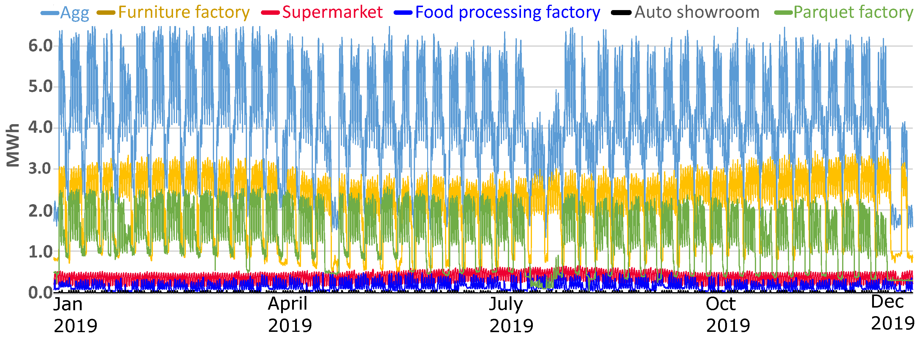
Figure 2 illustrates the structure of the cluster for the consumers analyzed in this study. Our case study analyses the approach of an energy supplier that manages a complex portfolio. The supplier has two options: (i) to forecast each consumer and add the forecasts; (ii) to forecast the aggregate load curve of the total cluster. We analyze both options and conclude the best scenario based on power market conditions and prices. Concluding that predicting each consumer results in higher errors, then it is more suitable to aggregate load curves and forecast. By doing so, the supplier will have fewer balancing costs and will be able to reduce the price to the consumer.
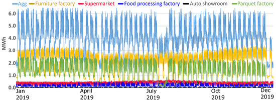
Figure 2.
Load curves of industrial and commercial consumers. Agg: aggregate consumption. The structure of the cluster (2019 annual consumption). PF = parquet factory; FF = furniture factory; SM = supermarket; FPF = food processing factory; AS = auto dealer.
In our study, we work with three manufacturing factories and two commercial consumers. From discussion with the consumers, we identified similar issues as pointed out by [32] mentioning that industrial and commercial consumers have little awareness about the energy footprint; additionally, we identified a small interest for energy costs, is regarded as a non-controllable cost. The authors in [33] present the behavior of industrial and commercial consumers and price elasticity.
The aggregated forecasts are used to simulate electricity acquisition from the day-ahead market, and the forecast errors are correlated with quantity and the cost on the balancing market. In this manner, we evaluate the hourly impact of forecasts on the power market. The aggregated forecast is compared with individual forecasts to understand the best approach in minimizing the errors. The work presented by [34] explain how to analyze the aggregate electricity consumption of many consumers and extract key components such as heating, ventilation, and air conditioning (HVAC), residential lighting, and street lighting consumption from the total consumption.
2.2. Software Resources
The implementation of the forecasting methods is conducted in the Python development environment. For our project, we used Tensorflow [35], which is an open-source library developed for traditional and deep learning applications. Keras [36] is a high-level API, open-source library for machine learning that works on top of Tensorflow. For the data preparation and subsequent visualization of the results, Scikit-learn [37], Numpy [38], and Matplotlib [39] as well as Seaborn [40] libraries were used. The simulations computed on a PC Intel(R) Core(TM) i5-4690K CPU@3.5 GHz, RAM 16 GB, 64-bit operating system, x64-based processor.
2.3. Forecasting Using Traditional Methods
Autocorrelation diagrams indicates lag 1 with linear patterns distributed diagonally. As the level of autocorrelation increases, the points cluster more tightly along the diagonal. In Figure 3 we present the analysis for power consumption, and we can observe that for Auto Showroom (AS), there is a high level of non-linearity. From a forecasting point of view, the load curve of a supermarket is more accessible to predict than a parquet factory usage due to the characteristics of the electric equipment. This fact can clearly be observed in the forecasting results presented in Section 3. Forecasting errors for the SM load curve are lower by 1% MAPE in comparison with the other load curves because of the autocorrelation in past historical data.
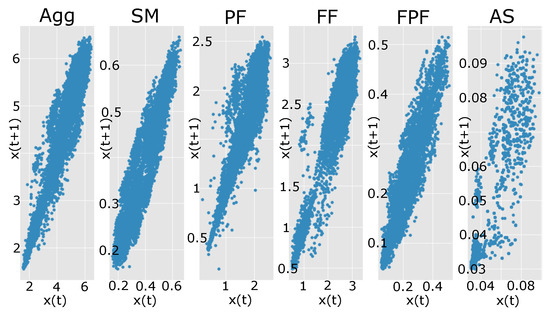
Figure 3.
Lag 1 applied for each time series for distribution analysis.
In order to have a comparison reference for STLF (short term load forecasting) we implemented established models to have a starting point in comparing results and showcasing the necessity for more complex approaches. Following Section 1.2, the naive methods implemented: (i) Hourly forecast for next day equals actual hourly values from the previous day as in Equation (1), (ii) Hourly forecast for next day equals actual hourly values from the same day last week Equation (2).
where, h. For weekends previous hourly values from Saturday and Sunday were used. For the Monday forecast, we considered past values from last Friday. For the holiday forecast, an average profile was constructed. After a long holiday period, the last working days represented the next forecasts.
where, h. Hourly values from the previous week become forecast for the current week correspondingly. For instance, for forecasting hourly values for next Tuesday, we use the values from past Tuesday.
The moving average applied for hourly values from the past day and two weeks ago according to Equation (3). These simple methods define a benchmark for the next forecasting methods and showcase the real-life forecasting approach from most suppliers.
In the autoregressive model, the electricity usage in the previous period has become the predictors. An autoregression relation is a number of immediately preceding values in the series that predict the value at present. The AR model uses 14th-order autoregression AR(14) to analyse relevant predictors for the next 24 h. The only exogenous factor with relevant statistical p-value is temperature for the supermarket load (p-value = 0.0023).
Based on the p-value scoring presented in Table 1, we keep the past hours that are relevant for the regression Equaton (4). All the previous steps that have scored above 0.05 for p-value are removed from the regression equation. forecast is made based on the previous values.

Table 1.
Regression Statistics. .
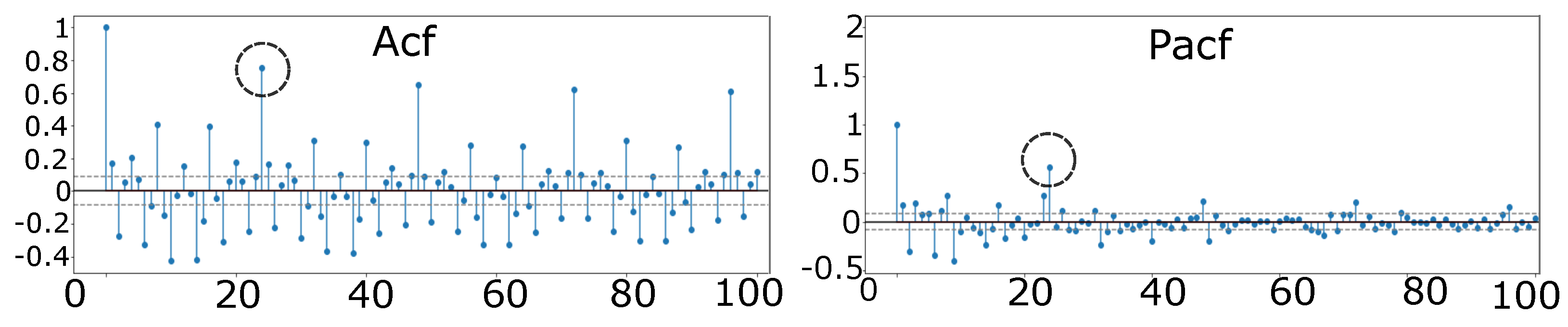
For seasonal ARIMA, a similar approach was implemented by [41], who used the seasonal factor of 24; in this study, we have found that using data from the last week produces better results, so we choose a cyclical factor of 24. Analyzing the auto-correlation (ACF) and partial autocorrelation (PACF) plots of the series, the first significant value at lag 2 for ACF and lag 2 for the PACF, which suggest using p = 2 and q = 2. Significant values appear at lag 24 in the ACF plot which suggests our cycle is S = 24 (according to Figure 4). The diagrams for ACF and PACF represent the values for the aggregated load curve. The time series analyzed are not differenced because it is a stationary series; the method used for SARIMA has the following order (2,1,2) (1,0,0) [24].
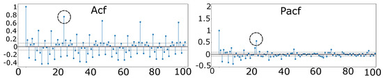
Figure 4.
Autocorrelation and partial autocorrelation functions.
According to equations for triple ES, we implement the algorithm for hourly values in order to make our predictions for the next 24 h. We use t = 24 periods in each day, meaning that the initial factors can be calculated with Equation (5):
We obtain the predicted values for the next batch of 24 h. The coefficients corresponding to each component are = 0.9331, = 0.0014, = 1. These values for the coefficients were obtained by using Solver application in Excel, which are similar to the values obtained by using python and statsmodels v0.12.2.
2.4. Forecasting Using Machine Learning
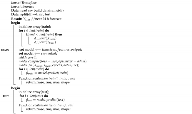
For the implementation of the ML methods with supervised learning, we follow the same framework presented in Algorithm 1 for each algorithm. The data comes from reliable sources and does not need preprocessing. The first step is to upload the .csv file in Jupyter Notebook. Then the data is split into 80% training and 20% testing. The last step before training the NN is to arrange the data in the form of multi-dimensional arrays. The data are normalize with min–max scalar function from [37].
| Algorithm 1: Machine learning forecasting algorithm (h = forecast horizon) |
 |
Various methods and models are implemented in this article for load forecasting (LF) which give different results depending on the type of load. There are three main categories of electric loads according to [42], and Ref. [43] exemplifies macro-categories between types of consumers: industrial, commercial, residential, and public authorities. The load curve of each category has a different pattern of time series hourly demand. Industrial consumers being the hardest to predict due to the multitude of devices and equipment used by employees throughout the working day. Industrial load curves are less deterministic, and daily or hourly patterns have high volatility spikes and dips. In this article, the hyperparameters used are presented in Table 2. Literature indicates that electric load time series are often simultaneously linear, nonlinear, seasonal, nonseasonal, and uncertain patterns. A comprehensive model and methods for LF must work on all patterns and features.
Table 2.
Parameters used by the forecast methods implemented in this work.
2.4.1. Multilayer Perceptron (MLP)
MLP is a type of feedforward neural network composed of multiple layers of perceptrons (with threshold activation) [44]. The MLP is a very popular form of artificial neural networks applied to both regression and classification problems. MLP can be interpreted as nonlinear function mapping from the inputs to the outputs.
The MLP consists of an input layer, followed by one or more hidden layers comprised by nonlinearly-activating neurons (nodes), and an output layer. Most used activation functions are , sigmoid function , ReLU, Linear, Softmax, Exponential Linear Unit [45].
In this work, we use an architecture composed of 24 inputs, multiple hidden layers with N neurons, and 24 neurons in the output layer. The choice of this configuration relies upon its ability to perform best-fit approximations of continuous functions on input and output subsets. In the learning process, the weights are constantly adapted based on the Gradient Descent algorithm.
2.4.2. Recurrent Neural Networks
One of the early implementations of RNN (recurrent neural network) was proposed by [46] for 1 h ahead forecasting and [47] showing that RNN is superior to FFNN (feed forward neural network).
A recurrent correlation is an equation that defines an element of a sequence as a function of previous elements of the same sequence Equation (6). Recurrent networks define such recurrence relations, and therefore they are called recurrent neural networks. The states in the recurrent net are the encodings of the hidden units, typically denoted as vectors with associated time step. The state sequence is dependent on the previous states. Additionally, the state sequence is also affected by the input at each time step and the parameter . Thus, the recurrent relation for the recurrent neural network is:
Once the state of the system has been inferred this way, the output at any time step is a function of that state as:
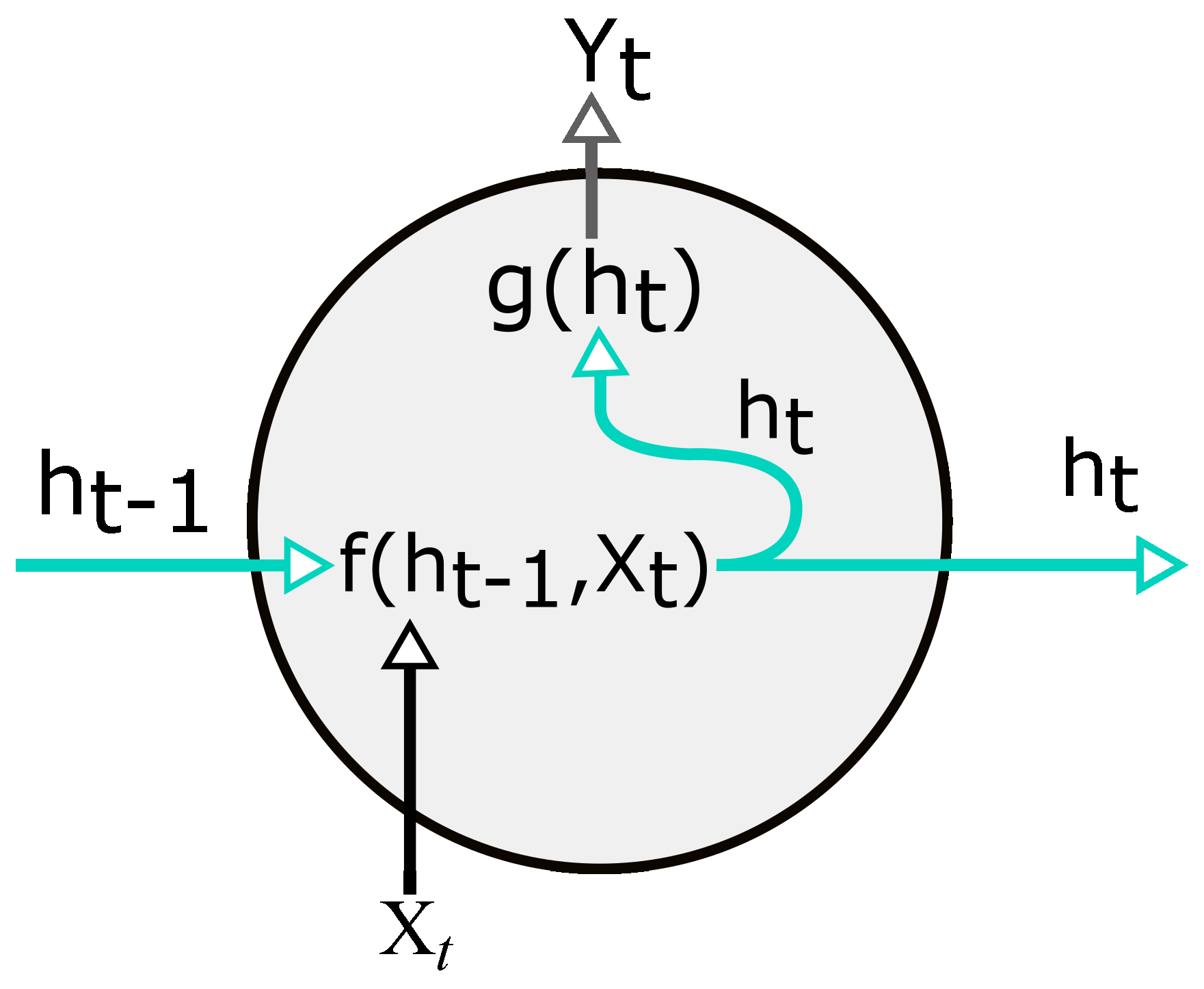
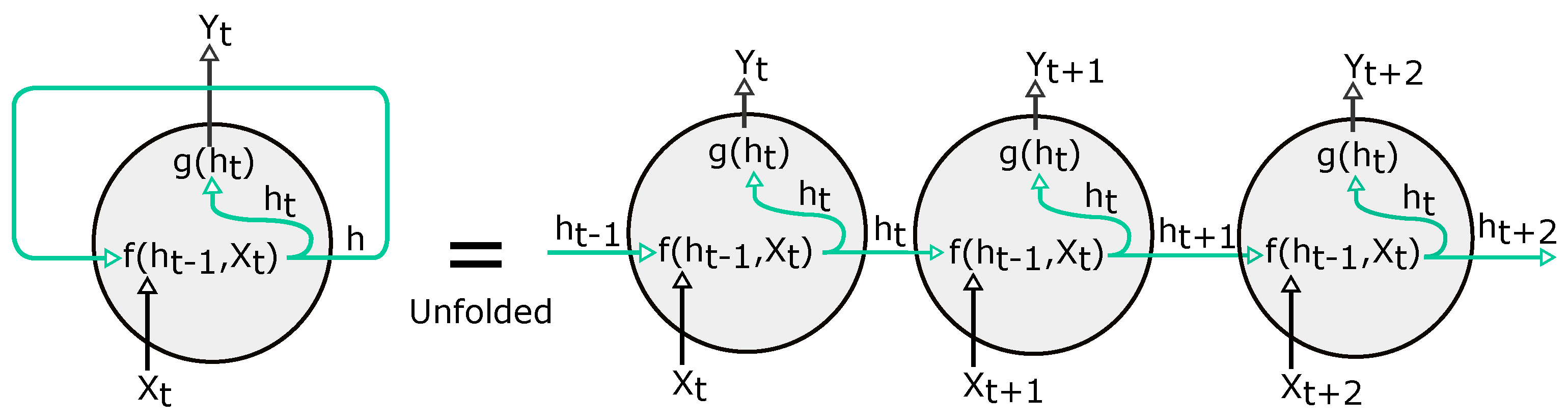
where is a different set of parameters, specifically trained for the output variable. The functions f and g are applied at each time step and collectively are known as RNN cell (Figure 5), a repeatable unit in the network.
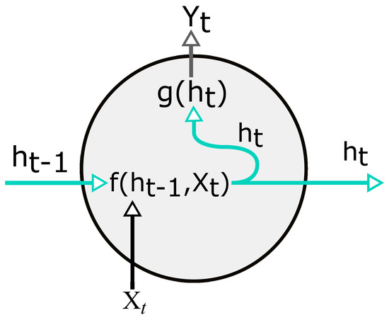
Figure 5.
RNN cell. Array X and array Y represent the input and output of the network; h indicates the hidden units of the network; t represents the time point.
For neural networks to define functions is to obtain an output by multiplying a weight vector to the input vector, add bias, and then apply the activation function to allow the modeling of non-linearity in the output. To assume the current state, we can use a simple version of function f (8).
In the equation above, the parameters include W, U, and b. The W and U are parameters representing weight matrices for inputs and states. Values for the bias b are organised in a vector. To address non-linearity, the hyperbolic tangent is used as an activation function (tanh); other activation functions could be used. The output of the RNN cell is:
where V and c denote the weight and bias, the parameters of the output function g. Matrix V and vector c will determine multidimensional outputs. The same set of parameters is applied at each time step for every RNN-cell.
Writing a recurrence relation for all input variables is known as unfolding the network as presented in Figure 6. Unfolding shows the hidden state at any time t as a function of the parameters and the entire sequence up to the point t, . For forecasting a standard RNN computes a sequence of outputs by iterating Equations (8) and (9), where m is the forecast horizon. To train an RNN, we have to infer . During the forward pass, we have to compute through all the hidden states h(1),…,h(t) to derive the gradients of the parameters of the model. The computational graph calculates the hidden state at each time step and stores it to compute the gradients. Then, the computation of gradients using BPTT (backpropagation through time), starting at a loss and then sequentially going backward in time from the gradient of the hidden variables h(t) to the gradient of h(1).
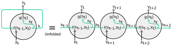
Figure 6.
Folded and unfolded regular RNN.
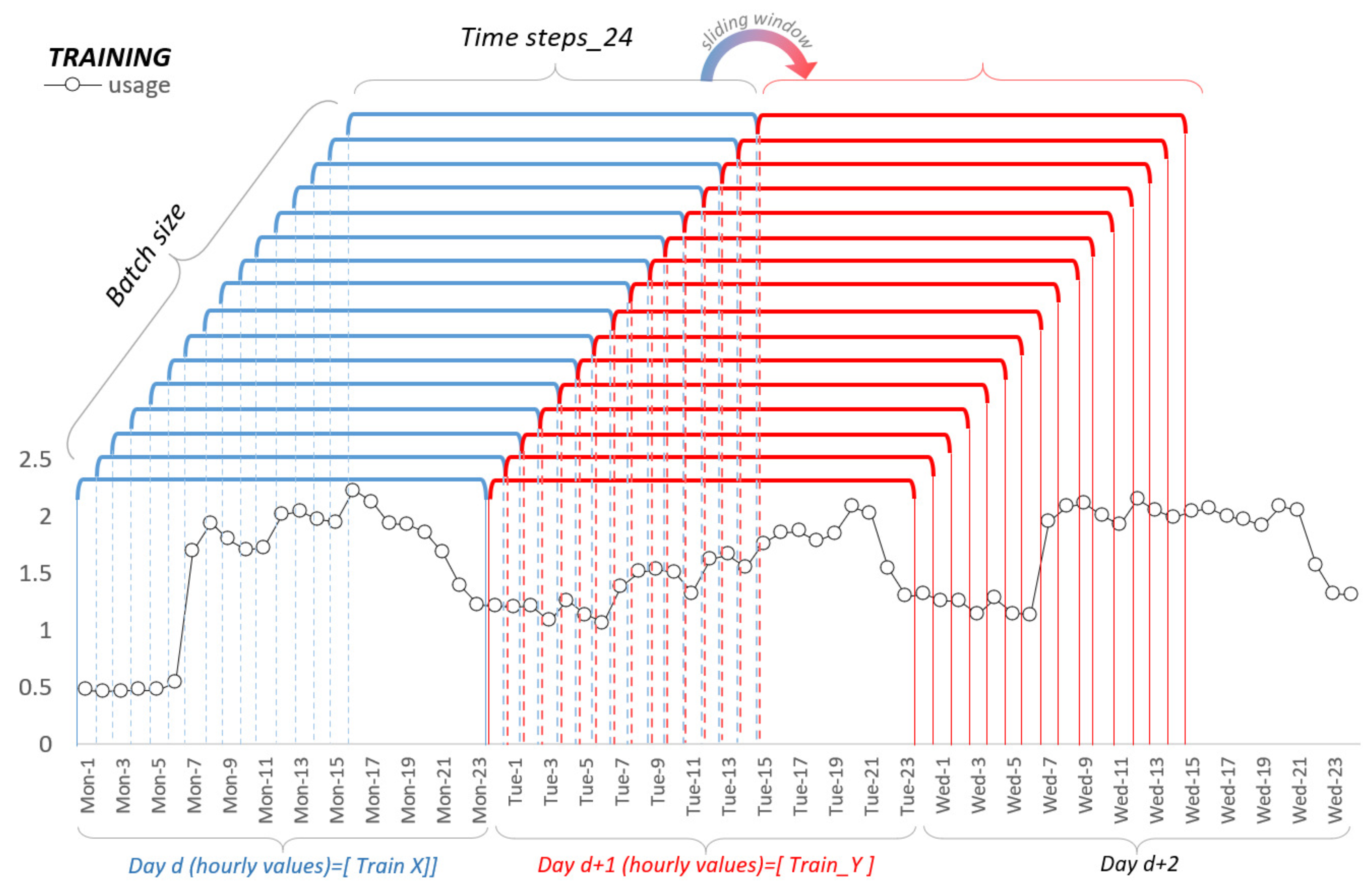
In our work, we approach time series forecasting as a supervised learning. The sequential supervised learning is described by [48] and can be formulated as follows: Let be a set of N training examples. Each example is a pair of sequences , where and . The task is to predict the t + 24 elements of a sequence . This can be extended in two ways. First, consider the case where each is a vector . The time-series approach becomes a matter of mapping simultaneously a batch of parallel time series: Predict given . Second, we use exogenous variables if relevant to . A detailed illustration of these processes is presented in Figure 7:
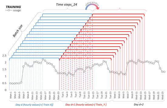
Figure 7.
Sliding window for training.
The computation of RNN has N sequential inputs and sequential outputs. In the following mathematical representation of the RNN model computational graph, the number of layers is denoted as L from 1 to N. The activation function is denoted correspondingly to L as :
Prediction is achieved by inserting batches of 24 inputs from the previous day, including the exogenous variables to the network and forecast the following 24 values (hours), as presented in Figure 8.
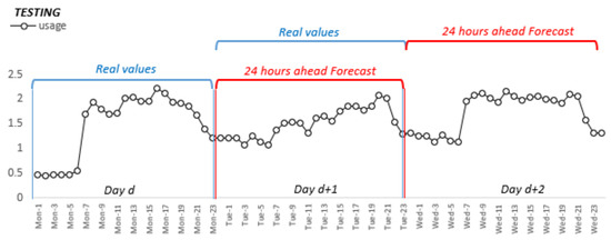
Figure 8.
Forecast horizon window for testing data.
2.4.3. Long-Short Term Memory
LSTM (long-short term memory) has been popular since [49] presented them as a solution to the vanishing and exploding gradient. Approaches have been implemented in a variety of domains, the authors of [50] applied the method for load forecasting, and various models were developed by [51] for horizons of 24 h, 48 h, 7 days, and 30 days and applied for residential customers [52] the implemented RNN architectures. The literature is rich in reviews of deep learning algorithms [53,54,55], also, many comparisons between architectures are studied [56].
Training an LSTM network, we need a few key parameters as in Table 3, provided in Keras [36], that will determine how the network performs.
Table 3.
LSTM model parameters.
The batch size limits the number of input values to the network before a weight update. This same limitation is then imposed when making predictions with the fit model. The concept for supervised learning presented in Figure 7 and Figure 8 is applied for all the ML methods implemented for this article.
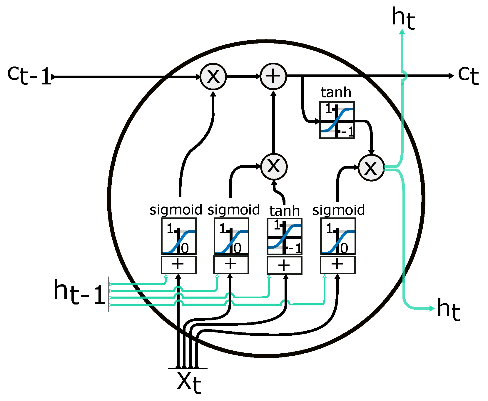
In the model of LSTM, there are internal self-loops for storing information. There are five essential elements in the computational graph of the LSTM: (1) input gate, (2) forget gate, (3) output gate, (4) cell, and (5) state output. Figure 9 shows the LSTM computational model in the cell layer, and these are combined with other cells to form the RNN model. The gates operations, such as reading, writing, and erasing, are performed in the cell memory state. The following equations show the mathematical representation of the model:
where is the input of the input gate, is the input of the forget gate, is the input of the output gate, U is the update signal, is the state value at the time t and ht is the output of the LSTM cell. The memory state can be modified by the decision of the input gate using a sigmoid function with an on/off state. If the value of the input gate is minimal and close to zero, there will be no change in the state cell memory . The stacked LSTM can be represented in multi layers in the network model.
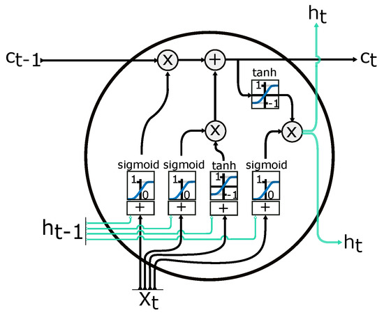
Figure 9.
RNN LSTM cell. —input vector; —memory from current cell; —memory from previous block; —output from current cell; —memory from previous cell; —element-wise multiplication; —element-wise summation/concatenation. Adapted from [57].
2.4.4. Gate Recurrent Unit (GRU)
Another type of recurrent neural network, a simplified version of the LSTM cell, is illustrated in Figure 10. The network is applied by the authors in [58] on aggregated loads to obtain a MAPE of 1.13%. GRU are simpler than LSTM, as they use one less gate and eliminate the need for distinguishing between hidden states and memory cells. RNN, sequence to sequence architectures and temporal convolutional neural networks applied by authors in [59] examine data for a single household and several aggregated meters. The findings show that the simple RNN performs comparably to GRU and LSTM when adopted in aggregated load forecasting. The best results are an RMSE equal to 13.8, and MAE equal to 7.5, generated by the LSTM.
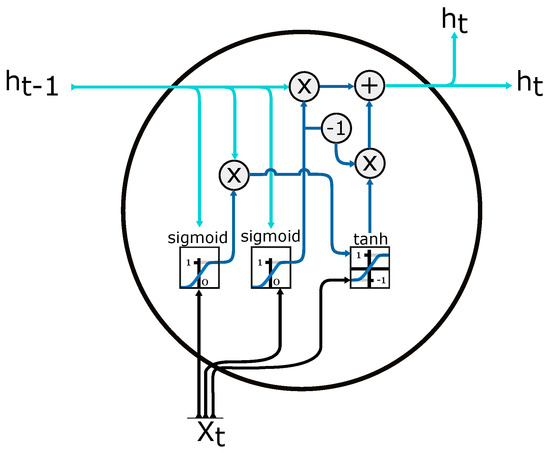
Figure 10.
GRU Gate Recurrent Unit cell. —input vector; —output from current cell; —memory from previous cell; —element-wise multiplication; —element-wise summation/concatenation. Adapted from [57].
In the case of STLF [60], they used a GRU with better average performance (mape of 2.82%) than LSTM(mape of 3.8%) for power load at the utility level.
2.4.5. LSTM Encoder—Decoder
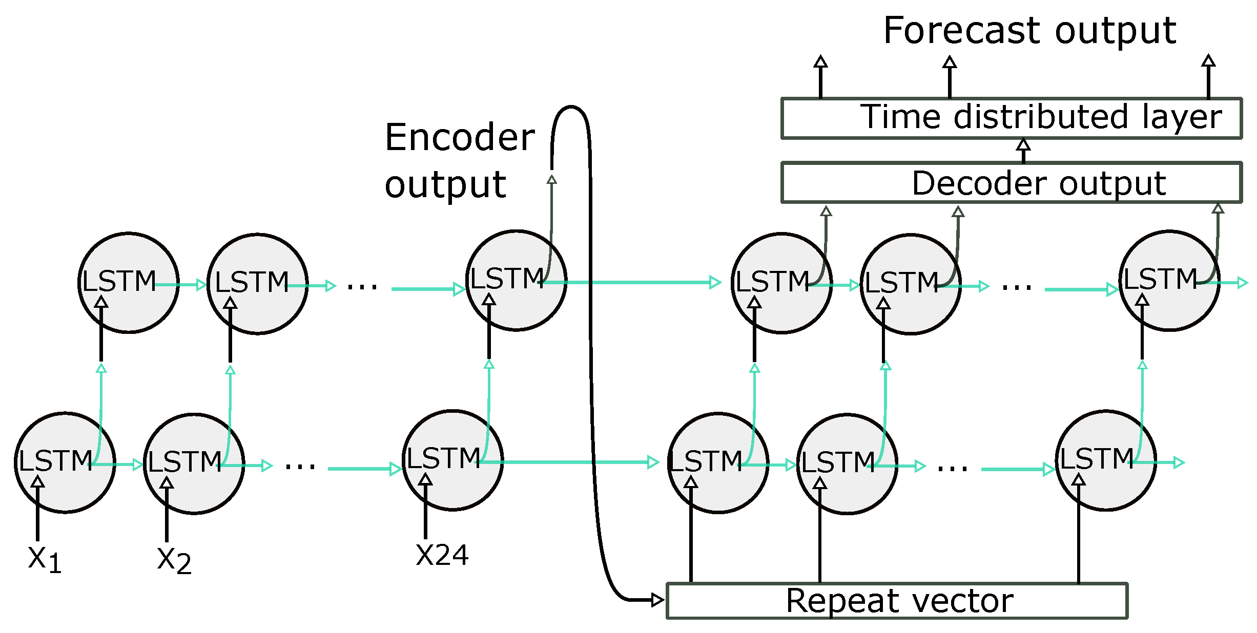
The Encoder–Decoder LSTM [61] is a recurrent neural network designed to address sequence to sequence data as presented in Figure 11. This model’s architecture comprises two parts: one for reading the input sequence and encoding it into a fixed-length vector, and a second for decoding the fixed-length vector and predicting the output sequence. The Encoder–Decoder methods have been introduced to sequence learning tasks for machine translation by [62,63]. An LSTM-based encoder maps an input sequence to a vector representation of fixed dimensionality as presented for the training stage in Figure 7. The decoder is another LSTM network, which uses this vector representation to produce the target sequence.
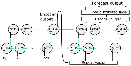
Figure 11.
LSTM Encoder Decoder architecture.
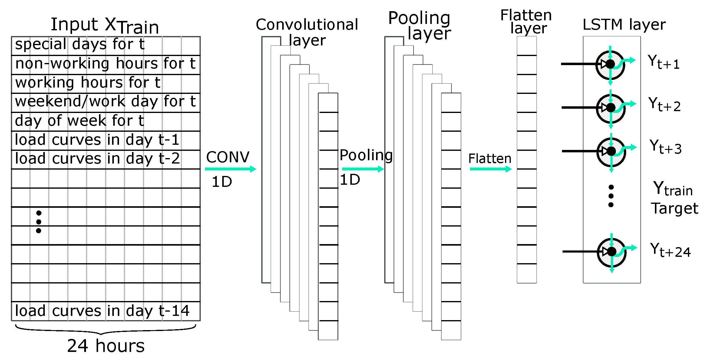
2.4.6. CNN (Convolutional Neural Network)—LSTM Arhitecture
The CNN-LSTM architecture involves specific layers for feature extraction on input data combined with recurrence to support sequence prediction. CNN-LSTM works better for visual time series prediction problems and the application of generating textual descriptions from sequences of images [64]. For forecasting time series models, the capability to extract temporal and spatial features allows for the LSTM layer to memorize sequential dependencies in time. In contrast, the CNN layer informs this process through the use of dilated convolutions as illustrated in Figure 12. Ref. [65] indicates that LSTM performance can be optimized by carefully extracting features to the LSTM. In this case, the CNN layers reduce the spectral variance of the time series.
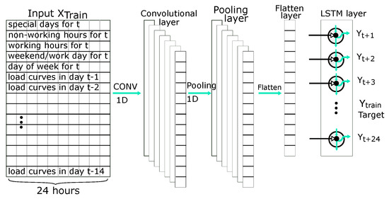
Figure 12.
Structure of CNN—LSTM.
The input to the CNN layer is past hourly usage and other features such as day of the week, working or non-working days/hours, and special days. The output of the input layer extracts features for the LSTMs and several hidden layers. The hidden layer typically consists of a convolution layer, an activation layer, and a pooling layer. The convolution layer applies the convolution operation to the incoming multivariate time series sequence and passes the results to the next layer.
3. Results
The first step to minimize the cost generated by imbalances is to evaluate it. We analyzed the best practices for LF, considering the activity of an energy supplier on the power market. The forecasting algorithms use the parameters from Table 2. For the evaluation of the forecasted results, well-known metrics (Table 4) are used and correlated with the effectiveness of forecasts in the context of the power market for the period in which we tested the forecasting algorithms. We build the scenarios based on buying the entire energy from the Day Ahead Market (DAM). This is a real scenario for an energy supplier but, usually, an energy portfolio is much more complex and diverse; in our simulation, we try to showcase the impact of error metrics and energy portfolio imbalances. Differentiating between forecast and actual values () will determine the imbalance of quantities that will be settled on the BM. If , meaning that the forecast is higher than the actual values, the surplus needs to be sold on the BM. If , meaning that the forecast is lower than the actual values, the deficit needs to be purchased from the BM.
Table 4.
Forecast errors metrics.
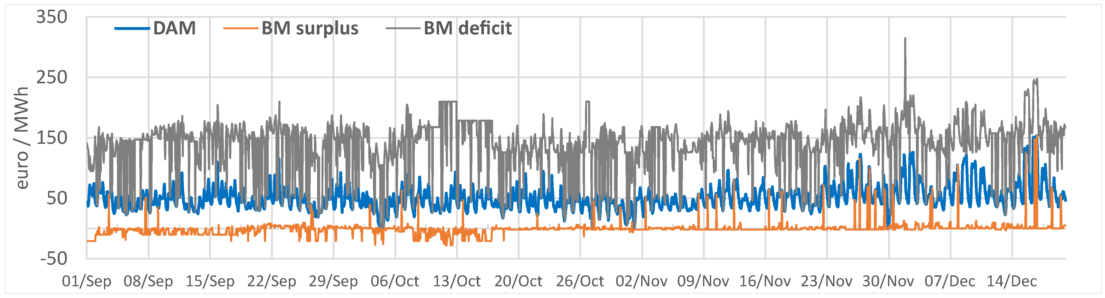
To achieve this simulation, we apply Equation (17) hourly for the forecast and actual values, simulating power market activity. Usually, buying from the BM is very expensive and selling at low or negative prices. In Figure 13, we present the prices considered in our analysis for each forecasting method. The forecast is the notified quantity on the DAM. We calculate the imbalance and determine the surplus or deficit of electricity (on an hourly basis) by comparing the forecast with the actual values in the testing period. This procedure applies to every algorithm implemented in this article, both for the aggregated and individual forecasts.
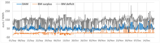
Figure 13.
Hourly prices euro/MWh for the DAM and BM from the Romanian power market operator. The exchange rate for conversion to euro in Q4 2019 is 4.7665 lei/euro. https://www.bnro.ro/Raport-statistic-606.aspx accessed on 28 August 2021.
To calculate the hourly cost of electricity (), in our scenario, we use the hourly prices from Figure 13:
where , , , represent the hourly price for DAM, surplus and deficit (Figure 13). The cost is initially calculated on an hourly basis, and in the end, is summed up for the entire period of testing. Further, we present the traditional metrics used for forecasting evaluation.
Results analysis presented in Table 5 show that errors are higher for individual forecasting. The lowest errors with MAPE 5% are obtained by applying ML methods for the aggregated and individual consumption in the testing period. Forecast errors for the supermarket load curve are the lowest at 4.20%. The reason for this is the linear characteristic of the past time series and correlation with temperature, as in Figure 3. A supermarket uses electricity for equipment that operates every day in the same manner, and the only exception is few days per year for holidays. The largest consumer for a supermarket is the refrigeration installations, which are dependent on the temperature and the number of clients in the selling area.
Table 5.
Results for 24 h ahead forecasts for aggregated and individual load curves.
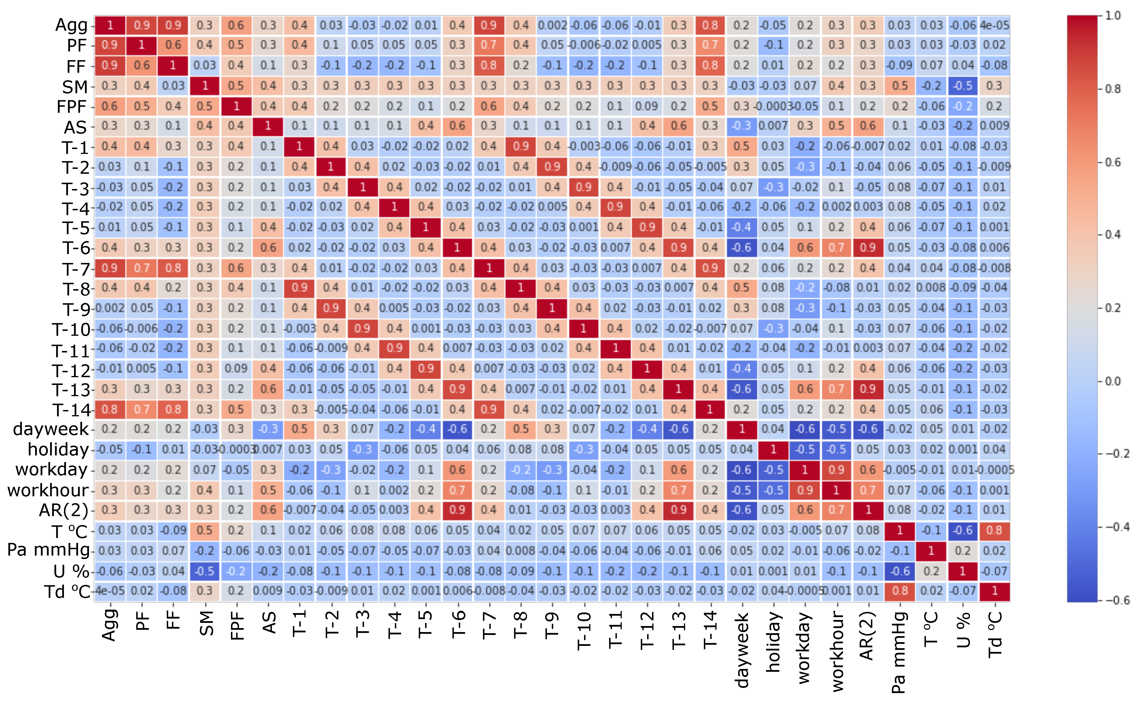
The temperature was used in the forecast, as shown in Figure 2 in the summer period because of high temperature the consumption rises due to the demand for air conditioning. The food processing plant presented in this study has refrigeration installations, but we could not find a correlation with temperature. Figure 14 illustrates the exogenous variables considered in this study by a heatmap correlation diagram that illustrates the correlation between the variables.

Figure 14.
Auto regressive elements and exogenous variables used in forecast.
In the case of the large industrial consumers, parquet factory (GRU MAPE—13.82%), and furniture factory (GRU MAPE—4.71%), which impact the load aggregation, it was challenging to identify the relevant exogenous variable that can influence the consumption pattern. The high error for the PF is because the factory has old equipment, and frequent breakdowns occur. Two weeks per year, the factory also has a general revision when the consumption behavior is highly volatile, as seen in Figure 2. The production flow is mainly based on electric motors that power machinery which processes raw wood until the final product. Both factories had large ventilated storage for drying the wood, but no relation could be established between outdoor dew temperature or humidity. Even working/non-working days are not the same because factory planning is dependent on production quota. The dependency on temperature is low because the thermal energy is produced, in our cluster, by burning natural gas or wood scraps. Despite development in forecasting methods, none can be generalized for all demand patterns [66]. When dealing with commercial or residential consumers, the forecasting methods can use exogenous variables such as temperature, humidity, solar radiation, or precipitation. Ref. [67] presents exogenous variable’s impact in the load forecast. In article [68], the authors highlight that using temperature as an exogenous variable does not improve the accuracy of the weekday’s prediction.
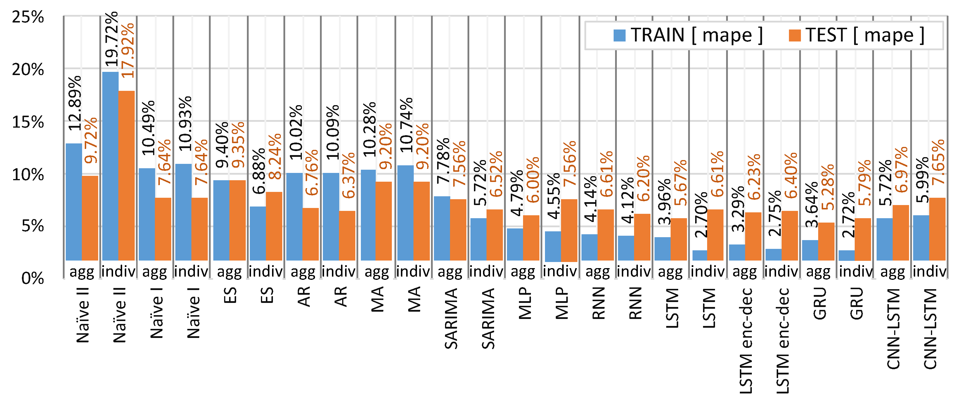
In this article, using temperature for the traditional methods result in higher errors. For the ML approach, temperature improved the forecast, humidity, and dew point are excluded from the training dataset. The AR method has the lowest errors (Agg—6.76% MAPE) compared to other traditional methods for the aggregated and individual load curves (SM—4.20% MAPE). To compare which approach is more advantageous for an energy supplier, we analyzed forecasting the aggregated load curve in contrast with summing up individual load forecasts. In Figure 15 each algorithm was applied to the dataset (train and test) to highlight the best practice for forecasting. Forecasting the aggregated load curve gives lower errors, especially for the ML methods. In none of the cases presented, the individual forecasts resulted in a lower error than the aggregated approach. The GRU aggregated result improved the result in comparison to the individual forecast by 8.81%.
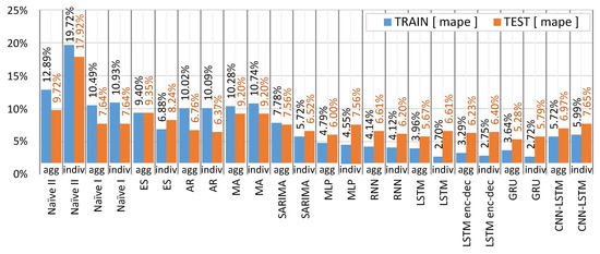
Figure 15.
Aggregated forecast (agg) compared to the individual forecasts (indiv).
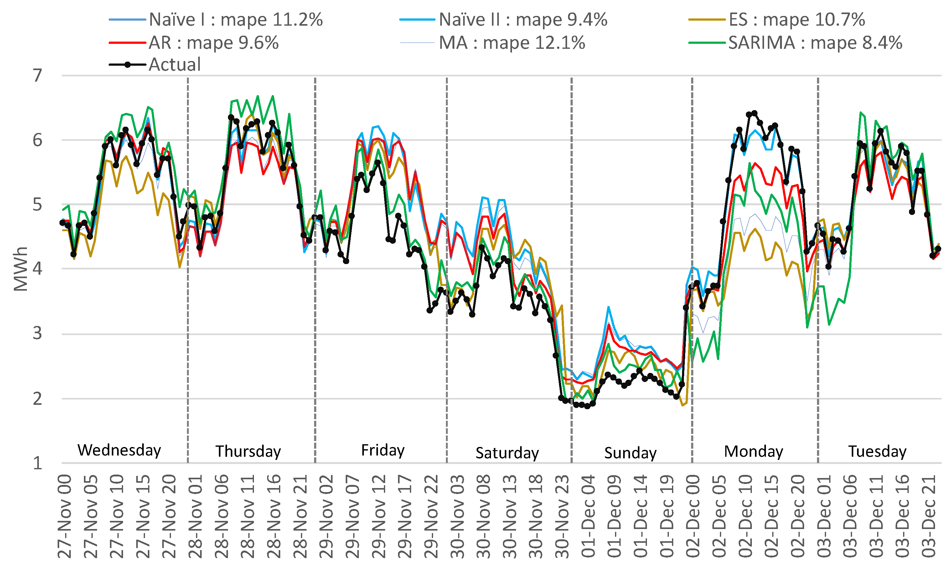
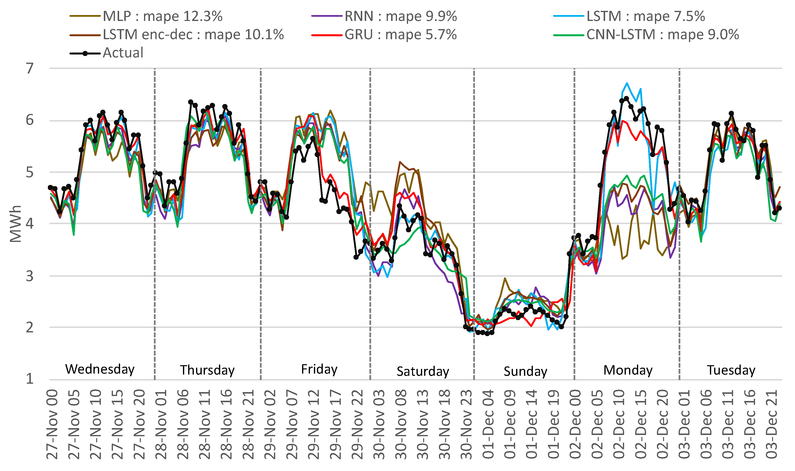
Because applying the forecast algorithms on the aggregated consumption offers the lowest errors in our approach, the following figures present the results for the aggregated forecast. The most unfavorable period in the testing dataset was selected to compare the performance of the algorithms. The period from the date of 27 November 2019 (Wednesday) to 3 December 2019 (Tuesday) is uncommon because of two legal holidays (on the 30 November and 1 December) overlapping with the weekend. In a situation like this, employees usually take a day or two for a vacation to combine more free days. In Figure 16, it can be observed that from Friday the consumption start to drop, on Saturday is lower than usual, and Monday is higher than normal to recover the non-productivity days. Figure 16 presents the results of the traditional methods. Because this type of variation has not occurred previously, the algorithms fail to detect Friday, Saturday, and Monday except for ES and Sarima. The lowest error is obtained with Sarima of 8.4% better than the AR method, which has a better overall MAPE for the testing period. In Figure 17 the ML methods results are presented for the same period mentioned before. Similar to the traditional methods, because Friday is a working day, the ML methods forecast a higher consumption than actual. However, for Monday, because it follows a holiday, the algorithms wrongly identify a smaller consumption.

Figure 16.
Comparison of actual with forecasted consumption—traditional methods.
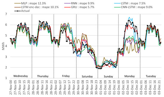
Figure 17.
Comparison of actual with forecasted consumption—ML methods.
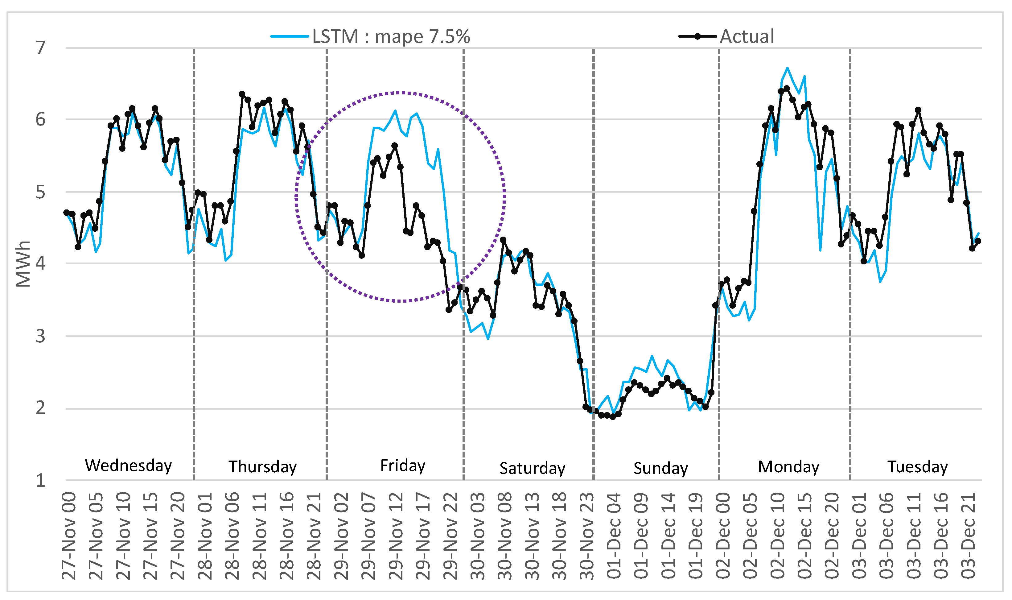
This outcome is similar to the traditional methods for the LSTM encoder–decoder, CNN-LSTM, RNN, and MLP. GRU and LSTM perform well in this period; Figure 18 and Figure 19 highlight a similar performance, but the GRU can better identify the load curve on Friday and Monday and outperform overall the LSTM.
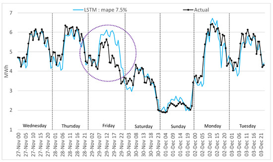
Figure 18.
Comparison of actual with forecasted consumption—LSTM.
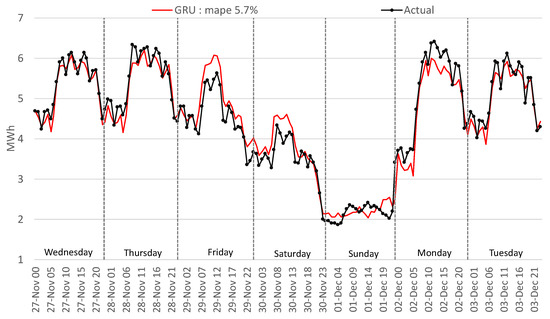
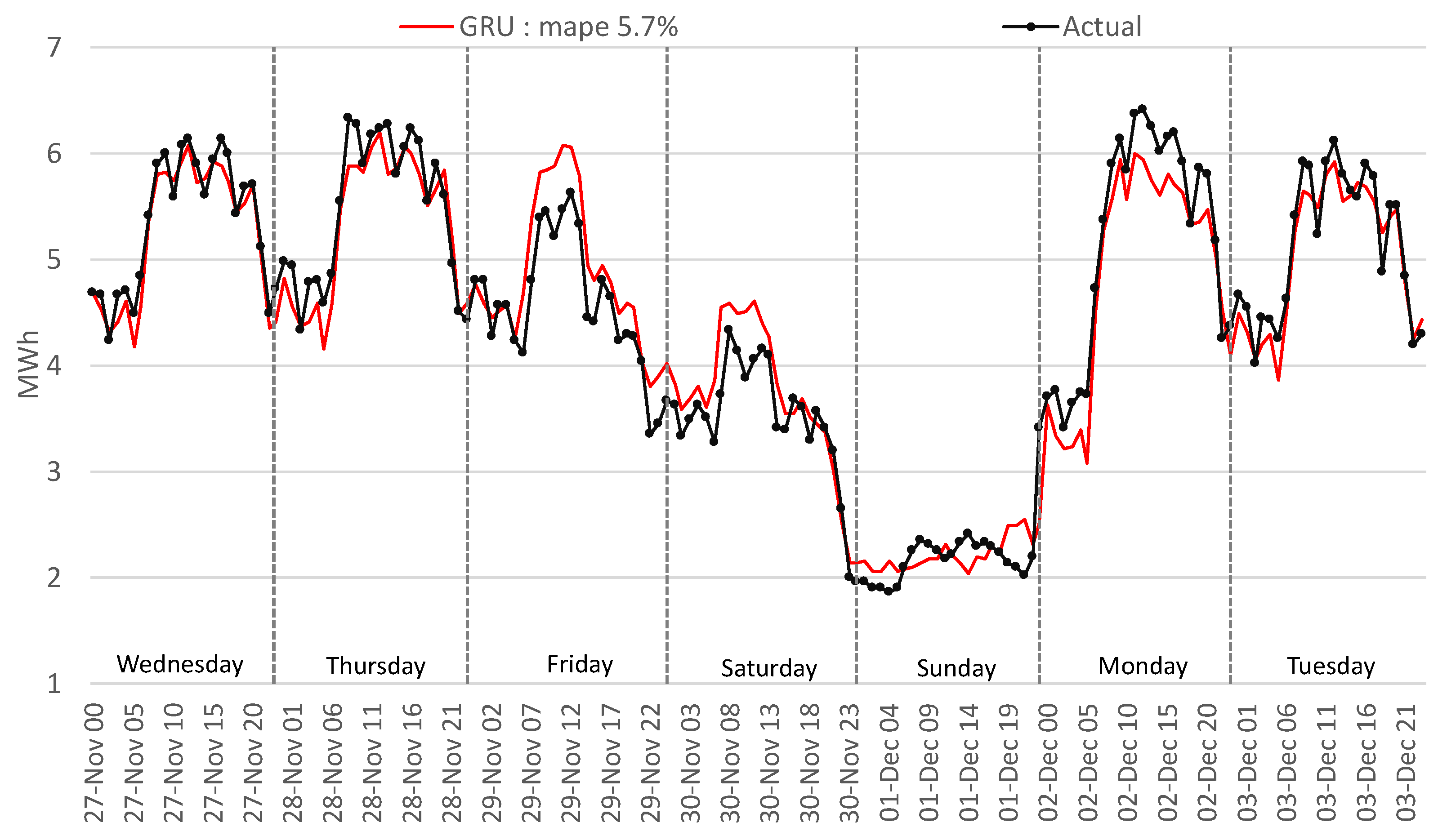
Figure 19.
Comparison of actual with forecasted consumption—GRU.
For the mentioned period, disappointing results were obtained (12.3% MAPE) with the MLP algorithm, worse than the traditional methods. The LSTM performs worse by 23.2% than the GRU method because of the overfitting of the network on the training data. Using fewer epochs to train the LSTM resulted in underfitting the training data. The GRU is a simplified LSTM network, trains faster, and therefore generalizes better on the training data. In Figure 18, the LSTM method interprets Friday as a normal working day, and in Figure 19 the GRU manages to minimize the gap between the actual and the forecasted values.
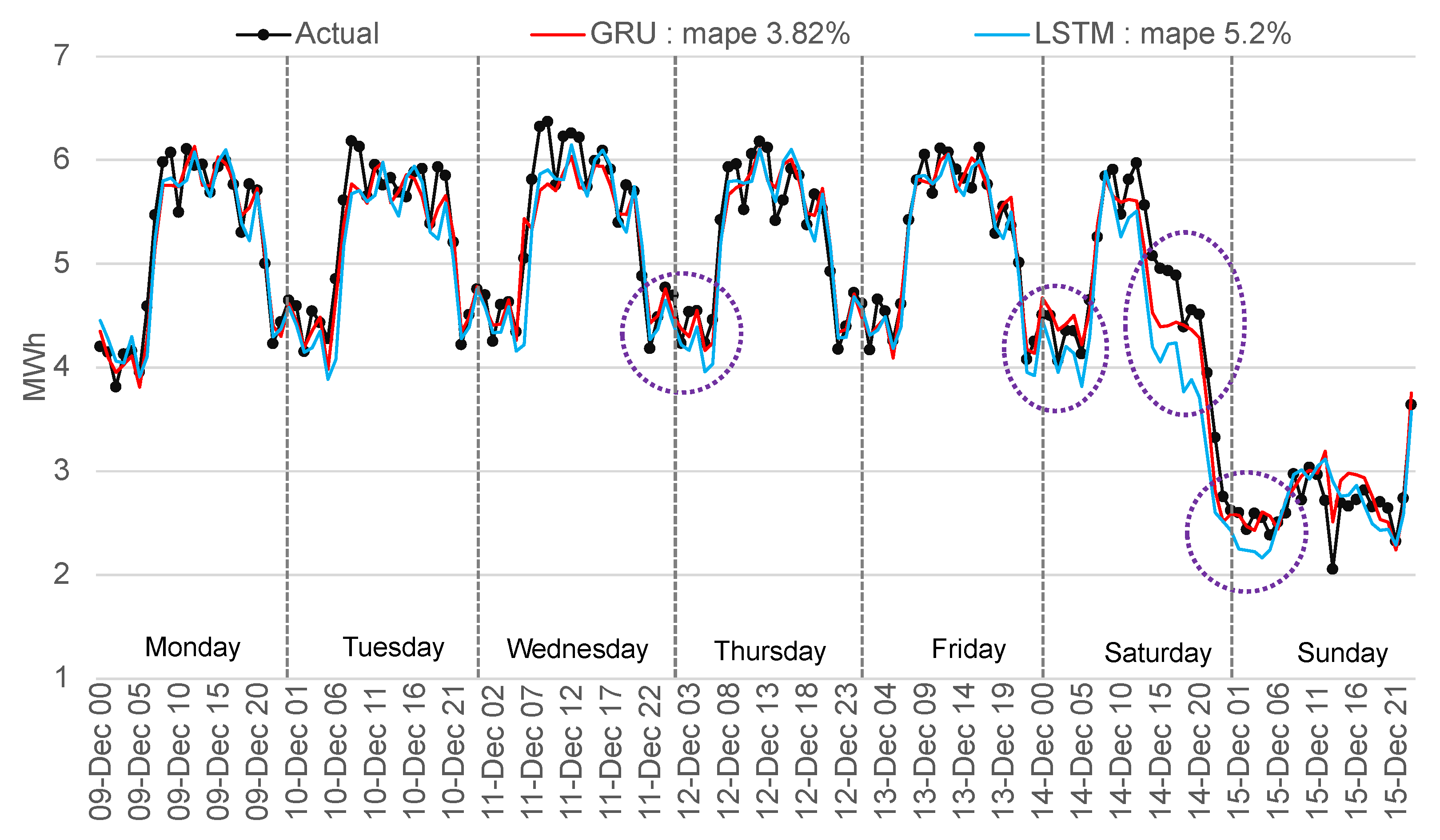
The GRU method forecasted with the lowest error the entire test period and confirmed the best performance for the unfavorable period from 27 November 2019 (Wednesday) to 3 December 2019 (Tuesday) with 5.7% MAPE. Another comparison is presented in Figure 20 for a normal week (from 9 December 2019 to 15 December 2019) to highlight the differences between the best-two methods implemented. The GRU forecast outperforms the LSTM by 26.59% with 3.82% MAPE, while LSTM scored a MAPE of 5.2%. For Saturday, it can be observed that the algorithms forecasted a much lower value of consumption, a situation explainable by the influence of the weekend from previous analysis with the legal holidays.
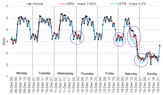
Figure 20.
Comparison of actual with forecasted consumption—GRU and LSTM.
The best-obtained result with a GRU network uses 20 inputs (past 14 days of hourly data, day of the week, working/non-working day and hours, special days, and temperature). The structure of the network comprises three hidden layers (200, 200, 168) trained for 100 epochs using the Adam optimizer for the gradient descent [69] and all the ML algorithms implemented mean square error for the loss function. The LSTM network that obtained the result presented in Figure 20 has the same structure as the GRU network mentioned in this paragraph. The results point out that, for high volatility time-series, GRU better approximates the changes through time without overfitting on high or low variations.
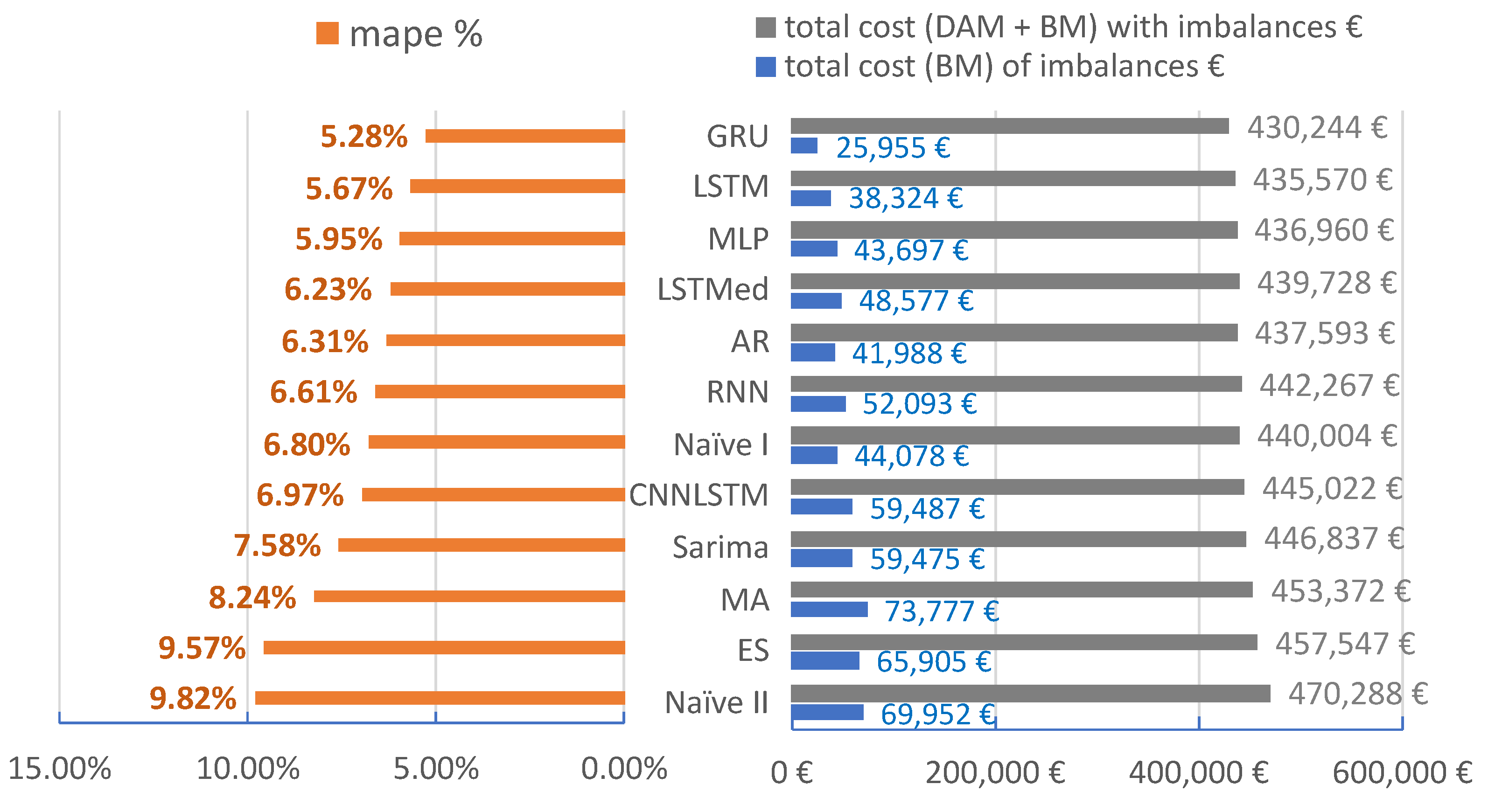
The purpose of our article is to demonstrate the practicality of machine learning to obtain short-term forecasts for aggregated industrial and commercial consumers. The forecasts are validated through various metrics and by calculating the Day-Ahead Market and Balancing Market impact. The novel approach is in determining the economic impact of forecasts. The forecasting errors mentioned in Table 4 are presented in Table 5 for the training and testing periods. Figure 21 quantifies the error metrics, based on Equation (17), in financial terms for the scenario presented. The costs presented are calculated hourly and are added for the testing period. The total value of cost from the best to the worst method increased by 8.51% (40.000 euro). By comparing the best two methods, the difference is 5326 euro, which means that using GRU, we lower the costs by 1.24% for the testing period. For a year, these costs can be four times higher depending on the evolution of the power market prices.
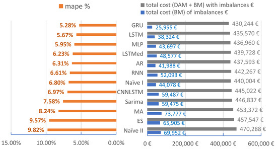
Figure 21.
Comparison of MAPE metric with the cost of the errors on the power market. The period analyzed is from 15 October 2019 to 20 December 2019. Total cost with imbalances includes the acquisition from the DAM and BM, and the total cost of imbalances represents only the cost generated by buying or selling on the BM.
4. Discussion
In this study, we implemented ML models to improve forecasting performance for a cluster of non-residential consumers. Our study compared the forecast performance for twelve methods and tested various combinations of forecast variables, lag structures, and aggregated versus individual forecasting. Our test sample results across 1608 hourly values (15 October–20 December 2019) indicates consistently that: (i) recurrent neural networks are suitable for industrial load consumption; (ii) the metrics for forecasting should be linked into power market context and preferable to simplify the approach for forecasting; and (iii) the best model implemented for aggregated load curves is GRU.
Comparing our best forecasting method with the best naive approach (used mainly by suppliers), we obtain a lower cost of 9760 euro for the three months in which we tested our models. This cost needs to be split for each consumer, but still, it is a cost that can be avoided. The best method implemented is GRU applied for aggregated loads resulted in 5.28% MAPE. Comparing GRU for the testing period of three months with the best statistical model, we obtain an improvement of 7.350 euro. The difference between GRU and LSTM is 5326.17 euro.
The novelty of our work is applying machine learning algorithms for an aggregated cluster of industrial and commercial consumers for forecasting 24 h. We propose a novel approach for evaluating the forecasting errors based on the costs that the errors generated in power markets.
5. Conclusions and Future Work
Our implementation handles three months of price data to validate forecast practicality with the Gated Recurrent Unit. We consider the current database sufficient. Our purpose for the future is to work with multiple consumers and apply demand response strategies with machine learning in future work. In 2019, the electricity settlement was hourly; from mid-2021, Romanian Energy Authority has changed the settlement interval to 15 min for the balancing market, which will increase the imbalance cost for suppliers. Already energy prices are high, but the 15 min settlement will increase the pressure on suppliers. The future development of this work will extend the forecasting horizon to multiple steps to enable the Intra-day Market and 15 minutes settlement on the balancing market in analysis. The main limitation in industrial load forecasting is the access to data. All the data used in this analysis are collected from the distribution power meters and obtained from suppliers. These consumers do not have energy monitoring systems, which would help a lot for forecasting. Another direction for development would be to find a partner with advanced smart metering and implement real-time forecasting. From a policy perspective, Romanian non-residential electricity consumers are not aware of the impact of forecasts or patterns of consumption on their electricity bills. Most non-residential electricity consumers in Romania have a single price per MWh. The consequence is that the industry does not carefully schedule production and is not actively communicating with the supplier. A possible policy would be to promote time of use tariffs, stimulated the consumer to follow a pattern, and better communicate with the supplier changes in production. Another implication for policy would be to increase energy efficiency programs and oblige all large consumers to invest in energy management systems capable of real-time measurement, for direct access to data.
Author Contributions
Conceptualization, S.U.; methodology, S.U.; software, S.U.; validation, A.C.C., V.T.; formal analysis, A.C.C., V.T.; investigation, S.U.; resources, S.U.; data curation, S.U.; writing—original draft preparation, S.U.; writing—review and editing, A.C.C.; visualization, S.U.; supervision, A.C.C. All authors have read and agreed to the published version of the manuscript.
Funding
Technical University of Cluj Napoca, Fiscal code: RO 22736939, Memorandumului Street no. 28, Cluj Napoca.
Institutional Review Board Statement
Not applicable.
Informed Consent Statement
Not applicable.
Data Availability Statement
Datasets for the DAM are publicly available from the market operator OPCOM (https://opcom.ro/opcom/pp/grafice_ip/raportPIPsiVolumTranzactionat.php?lang=ro accessed on 28 August 2021). The data for BM is collected from (https://www.opcom.ro/tranzactii_rezultate/tranzactii_rezultate.php?lang=ro&id=16). For the load curve dataset, restrictions apply to the availability of data. Only aggregated values and exogenous variables can be made available https://drive.google.com/file/d/1rec1NoXa05Y5yh_xCd-FNOHX4y33lMp6/view?usp=sharing. Hourly climatic data is obtained from the website: https://rp5.ru/Vremea_%C3%AEn_Baia_Mare_(aeroport) accessed on 20 August 2021.
Acknowledgments
This article was supported by the Project POCU/380/6/13/123927, “Entrepr-eneurial competencies and excellence research in doctoral and postdoctoral programs-ANTREDOC”, the project co-funded by the European Social Fund.
Conflicts of Interest
The authors declare no conflict of interest.
References
- Pellegrini-Masini, G.; Pirni, A.; Maran, S.; Klöckner, C. Delivering a timely and Just Energy Transition: Which policy research priorities? Environ. Policy Gov. 2020, 30, 293–305. [Google Scholar] [CrossRef]
- Koltsaklis, N.; Dagoumas, A.; Seritan, G.; Porumb, R. Energy transition in the South East Europe: The case of the Romanian power system. Energy Rep. 2020, 6, 2376–2393. [Google Scholar] [CrossRef]
- European Commission. A European Green Deal. Available online: https://ec.europa.eu/info/strategy/priorities-2019-2024/european-green-deal_en (accessed on 28 July 2021).
- O’Shaughnessy, E.; Cruce, J.R.; Xu, K. Too much of a good thing? Global trends in the curtailment of solar PV. Sol. Energy 2020, 208, 1068–1077. [Google Scholar] [CrossRef]
- Syranidou, C.; Linssen, J.; Stolten, D.; Robinius, M. On the Curtailments of Variable Renewable Energy Sources in Europe and the Role of Load Shifting. In Proceedings of the 2020 55th International Universities Power Engineering Conference (UPEC), Turin, Italy, 1–4 September 2020. [Google Scholar] [CrossRef]
- Ahmad, T.; Zhang, D.; Huang, C.; Zhang, H.; Dai, N.; Song, Y.; Chen, H. Artificial intelligence in sustainable energy industry: Status Quo, challenges and opportunities. J. Clean. Prod. 2021, 289, 125834. [Google Scholar] [CrossRef]
- Oprea, S.V.; Bâra, A.; Tudorică, B.; Călinoiu, M.; Botezatu, M. Insights into demand-side management with big data analytics in electricity consumers’ behaviour. Comput. Electr. Eng. 2021, 89, 106902. [Google Scholar] [CrossRef]
- Wang, S.; Sun, X.; Geng, J.; Han, Y.; Zhang, C.; Zhang, W. Application and Analysis of Big Data Technology in Smart Grid; IOP Publishing: London, UK, 2020; Volume 1639, p. 12043. [Google Scholar] [CrossRef]
- Zhang, M.; Lo, K.L. A comparison of imbalance settlement methods of electricity markets. In Proceedings of the 2009 44th International Universities Power Engineering Conference (UPEC), Glasgow, UK, 1–4 September 2009; pp. 1–5. [Google Scholar]
- ECOFYS Fraunhofer-ISI. Electricity Costs of Energy Intensive Industries—An International Comparison. Available online: https://www.isi.fraunhofer.de/content/dam/isi/dokumente/ccx/2015/Electricity-Costs-of-Energy-Intensive-Industries.pdf (accessed on 15 July 2021).
- Almeshaiei, E.; Soltan, H. A methodology for Electric Power Load Forecasting. Alex. Eng. J. 2011, 50, 137–144. [Google Scholar] [CrossRef] [Green Version]
- Winters, P.R. Forecasting Sales by Exponentially Weighted Moving Averages. Manag. Sci. 2021, 6, 324–342. [Google Scholar] [CrossRef]
- Taylor, J.W.; McSharry, P.E. Short-Term Load Forecasting Methods: An Evaluation Based on European Data. IEEE Trans. Power Syst. 2007, 22, 2213–2219. [Google Scholar] [CrossRef] [Green Version]
- Hyndman, R.; Athanasopoulos, G. Forecasting: Principles and Practice, 2nd ed.; Available online: OTexts.com/fpp2 (accessed on 29 April 2021).
- Box, G.; Jenkins, G.M. Time Series Analysis: Forecasting and Control; Holden-Day: San Francisco, CA, USA, 1976. [Google Scholar]
- Tao, Y.; Zhao, F.; Yuan, H.; Lai, C.; Xu, Z.; Ng, W.; Li, R.; Li, X.; Lai, L. Revisit Neural Network Based Load Forecasting. In Proceedings of the IEEE 2019, 2019 20th International Conference on Intelligent System Application to Power Systems (ISAP), New Delhi, India, 10–14 December 2019. [Google Scholar] [CrossRef]
- Djukanovic, M.; Babic, B.; Sobajic, D.J.; Pao, Y.H. Unsupervised/supervised learning concept for 24-h load forecasting. IEE Proc. Part C Gener. Transm. Distrib. 1993, 140, 311–318. [Google Scholar] [CrossRef]
- Upadhaya, D.; Thakur, R.; Singh, N. A Systematic Review on the Methods of Short Term Load Forecasting. In Proceedings of the IEEE 2019, 2019 2nd International Conference on Power Energy, Environment and Intelligent Control (PEEIC), Greater Noida, India, 18–19 October 2019; pp. 6–11. [Google Scholar] [CrossRef]
- Cai, M.; Pipattanasomporn, M.; Rahman, S. Day-ahead building-level load forecasts using deep learning vs. traditional time-series techniques. Appl. Energy 2019, 236, 1078–1088. [Google Scholar] [CrossRef]
- Moon, J.; Park, J.; Hwang, E.; Jun, S. Forecasting power consumption for higher educational institutions based on machine learning. J. Supercomput. 2018, 74, 3778–3800. [Google Scholar] [CrossRef]
- Božić, Z.; Dobromirov, D.; Arsić, J.; Radišić, M.; Ślusarczyk, B. Power Exchange Prices: Comparison of Volatility in European Markets. Energies 2020, 13, 5620. [Google Scholar] [CrossRef]
- Jierula, A.; Wang, S.; OH, T.M.; Wang, P. Study on Accuracy Metrics for Evaluating the Predictions of Damage Locations in Deep Piles Using Artificial Neural Networks with Acoustic Emission Data. Appl. Sci. 2021, 11, 2314. [Google Scholar] [CrossRef]
- Brownlee, J. Deep Learning for Time Series Forecasting. 2020. Available online: https://machinelearningmastery.com/machine-learning-with-python/ (accessed on 3 June 2021).
- Bellahsen, A.; Dagdougui, H. Aggregated short-term load forecasting for heterogeneous buildings using machine learning with peak estimation. Energy Build. 2021, 237, 110742. [Google Scholar] [CrossRef]
- Fekri, M.N.; Patel, H.; Grolinger, K.; Sharma, V. Deep learning for load forecasting with smart meter data: Online Adaptive Recurrent Neural Network. Appl. Energy 2021, 282, 116177. [Google Scholar] [CrossRef]
- Grigoras, G. 9—Impact of smart meter implementation on saving electricity in distribution networks in Romania. In Application of Smart Grid Technologies; Lamont, L.A., Sayigh, A., Eds.; Academic Press: Cambridge, MA, USA, 2018; pp. 313–346. [Google Scholar] [CrossRef]
- Guo, W.; Che, L.; Shahidehpour, M.; Wan, X. Machine-Learning based methods in short-term load forecasting. Special Issue: Machine Learning Applications To Power System Planning And Operation. Electr. J. 2021, 34, 106884. [Google Scholar] [CrossRef]
- Kim, J.; Moon, J.; Hwang, E.; Kang, P. Recurrent inception convolution neural network for multi short-term load forecasting. Energy Build. 2019, 194, 328–341. [Google Scholar] [CrossRef]
- Wu, W.; Liao, W.; Miao, J.; Du, G. Using Gated Recurrent Unit Network to Forecast Short-Term Load Considering Impact of Electricity Price. Innovative Solutions for Energy Transitions. Energy Procedia 2019, 158, 3369–3374. [Google Scholar] [CrossRef]
- Krstevski, P.; Borozan, S.; Krkoleva Mateska, A. Electricity balancing markets in South East Europe—Investigation of the level of development and regional integration. Energy Rep. 2021, in press. [Google Scholar] [CrossRef]
- Boechler, E.; Hanania, J.; Suarez, L.V.; Donev, J. Energy Education—Industrial Energy Use. Available online: https://energyeducation.ca/encyclopedia/Industrial_energy_use#cite_note-OED-1 (accessed on 15 May 2021).
- Moerenhout, T.S.; Sharma, S.; Urpelainen, J. Commercial and industrial consumers’ perspectives on electricity pricing reform: Evidence from India. Energy Policy 2019, 130, 162–171. [Google Scholar] [CrossRef]
- Otsuka, A. An Economic Analysis of Electricity Demand: Evidence from Japan. J. Econ. Struct. 2015, 28, 147–173. [Google Scholar] [CrossRef] [Green Version]
- Hobby, J.D.; Tucci, G.H. Analysis of the residential, commercial and industrial electricity consumption. In Proceedings of the 2011 IEEE PES Innovative Smart Grid Technologies, Perth, WA, Australia, 13–16 November 2011; pp. 1–7. [Google Scholar] [CrossRef]
- Abadi, M.; Agarwal, A.; Barham, P.; Brevdo, E.; Chen, Z.; Citro, C.; Corrado, G.S.; Davis, A.; Dean, J.; Devin, M.; et al. TensorFlow: Large-Scale Machine Learning on Heterogeneous Systems. 2015. Available online: tensorflow.org (accessed on 15 May 2021).
- François, C. Keras. 2015. Available online: https://keras.io (accessed on 15 May 2021).
- Pedregosa, F.; Varoquaux, G.; Gramfort, A.; Michel, V.; Thirion, B.; Grisel, O.; Blondel, M.; Prettenhofer, P.; Weiss, R.; Dubourg, V.; et al. Scikit-learn: Machine Learning in Python. J. Mach. Learn. Res. 2011, 12, 2825–2830. [Google Scholar]
- Harris, C.R.; Millman, K.J.; van der Walt, S.J.; Gommers, R.; Virtanen, P.; Cournapeau, D.; Wieser, E.; Taylor, J.; Berg, S.; Smith, N.J.; et al. Array programming with NumPy. Nature 2020, 585, 357–362. [Google Scholar] [CrossRef]
- Hunter, J.D. Matplotlib: A 2D graphics environment. Comput. Sci. Eng. 2007, 9, 90–95. [Google Scholar] [CrossRef]
- Waskom, M.; Botvinnik, O.; O’Kane, D.; Hobson, P.; Lukauskas, S.; Gemperline, D.C.; Augspurger, T.; Halchenko, Y.; Cole, J.B.; Warmenhoven, J.; et al. Mwaskom/Seaborn: v0.8.1 (September 2017); Zenodo: Genève, Switzerland, 2017. [Google Scholar] [CrossRef]
- Alberg, D.; Last, M. Short-term load forecasting in smart meters with sliding window-based ARIMA algorithms. Vietnam. J. Comput. Sci. 2018, 5, 241–249. [Google Scholar] [CrossRef]
- Andersen, F.; Larsen, H.; Boomsma, T. Long-term forecasting of hourly electricity load: Identification of consumption profiles and segmentation of customers. Energy Convers. Manag. 2013, 68, 244–252. [Google Scholar] [CrossRef]
- Chicco, G. Overview and performance assessment of the clustering methods for electrical load pattern grouping. Energy 2012, 42, 68–80. [Google Scholar] [CrossRef]
- Silva, I.; Spatti, D.; Flauzino, R.; Bartocci Liboni, L.; Reis Alves, S. Multilayer Perceptron Networks. In Artificial Neural Networks; Springer: Cham, Switzerland, 2017; pp. 55–115. [Google Scholar] [CrossRef]
- Mercioni, M.A.; Holban, S. The Most Used Activation Functions: Classic Versus Current. In Proceedings of the 2020 International Conference on Development and Application Systems (DAS), Suceava, Romania, 21–23 May 2020; pp. 141–145. [Google Scholar] [CrossRef]
- Mandal, J.K.; Sinha, A.K.; Parthasarathy, G. Application of recurrent neural network for short term load forecasting in electric power system. In Proceedings of the ICNN’95—International Conference on Neural Networks, Perth, WA, Australia, 27 November–1 December 1995; Volume 5, pp. 2694–2698. [Google Scholar] [CrossRef]
- Mori, H.; Ogasawara, T. A recurrent neural network for short-term load forecasting. In Proceedings of the Second International Forum on Applications of Neural Networks to Power Systems, Yokohama, Japan, 19–22 April 1993; pp. 395–400. [Google Scholar] [CrossRef]
- Dietrich, B.; Walther, J.; Weigold, M.; Abele, E. Machine learning based very short term load forecasting of machine tools. Appl. Energy 2020, 276. [Google Scholar] [CrossRef]
- Hochreiter, S.; Schmidhuber, J. Long Short-Term Memory. Neural Comput. 1997, 9, 1735–1780. [Google Scholar] [CrossRef]
- Cao, C.; Liu, F.; Tan, H.; Song, D.; Shu, W.; Li, W.; Zhou, Y.; Bo, X.; Xie, Z. Deep Learning and Its Applications in Biomedicine. Genom. Proteom. Bioinform. 2018, 16, 17–32. [Google Scholar] [CrossRef]
- Muzaffar, S.; Afshari, A. Short-Term Load Forecasts Using LSTM Networks. Innovative Solutions for Energy Transitions. Energy Procedia 2019, 158, 2922–2927. [Google Scholar] [CrossRef]
- Kong, W.; Dong, Z.; Jia, Y.; Hill, D.; Xu, Y.; Zhang, Y. Short-Term Residential Load Forecasting Based on LSTM Recurrent Neural Network. IEEE Trans. Smart Grid 2019, 10, 841–851. [Google Scholar] [CrossRef]
- Goodfellow, I.; Bengio, Y.; Courville, A. Deep Learning; MIT Press: Cambridge, MA, USA, 2016; Available online: http://www.deeplearningbook.org (accessed on 15 June 2021).
- Almalaq, A.; Edwards, G. A Review of Deep Learning Methods Applied on Load Forecasting. In Proceedings of the 2017 16th IEEE International Conference on Machine Learning and Applications (ICMLA), Cancun, Mexico, 18–21 December 2017; pp. 511–516. [Google Scholar] [CrossRef]
- Subbiah, S.; Chinnappan, J. A review of short term load forecasting using deep learning. Int. J. Emerg. Technol. 2020, 11, 378–384. [Google Scholar]
- Moroff, N.U.; Kurt, E.; Kamphues, J. Machine Learning and Statistics: A Study for assessing innovative Demand Forecasting Models. Procedia Comput. Sci. 2021, 180, 40–49. [Google Scholar] [CrossRef]
- Olah, C. Understanding LSTM Networks. Available online: http://colah.github.io/posts/2015-08-Understanding-LSTMs (accessed on 10 May 2021).
- Wu, D.C.; Bahrami Asl, B.; Razban, A.; Chen, J. Air compressor load forecasting using artificial neural network. Expert Syst. Appl. 2021, 168, 114209. [Google Scholar] [CrossRef]
- Gasparin, A.; Lukovic, S.; Alippi, C. Deep Learning for Time Series Forecasting: The Electric Load Case. CoRR 2019. Available online: http://xxx.lanl.gov/abs/1907.09207 (accessed on 13 April 2021).
- Li, X.; Zhuang, W.; Zhang, H. Short-term Power Load Forecasting Based on Gate Recurrent Unit Network and Cloud Computing Platform. In Proceedings of the 4th International Conference on Computer Science and Application Engineering, Sanya, China, 20–22 October 2020. [Google Scholar]
- Lim, B.; Zohren, S. Time Series Forecasting with Deep Learning: A Survey. 2020. Available online: http://xxx.lanl.gov/abs/2004.13408 (accessed on 3 May 2021).
- Cho, K.; van Merrienboer, B.; Gulcehre, C.; Bahdanau, D.; Bougares, F.; Schwenk, H.; Bengio, Y. Learning Phrase Representations using RNN Encoder-Decoder for Statistical Machine Translation. 2014. Available online: http://xxx.lanl.gov/abs/1406.1078 (accessed on 25 May 2021).
- Sutskever, I.; Vinyals, O.; Le, Q.V. Sequence to Sequence Learning with Neural Networks. CoRR 2014. Available online: http://xxx.lanl.gov/abs/1409.3215 (accessed on 22 May 2021).
- Donahue, J.; Hendricks, L.A.; Rohrbach, M.; Venugopalan, S.; Guadarrama, S.; Saenko, K.; Darrell, T. Long-Term Recurrent Convolutional Networks for Visual Recognition and Description. 2016. Available online: http://xxx.lanl.gov/abs/1411.4389 (accessed on 20 May 2021).
- Pascanu, R.; Gulcehre, C.; Cho, K.; Bengio, Y. How to Construct Deep Recurrent Neural Networks. 2014. Available online: http://xxx.lanl.gov/abs/1312.6026 (accessed on 5 June 2021).
- George-Ufot, G.; Qu, Y.; Orji, I. Sustainable lifestyle factors influencing industries’ electric consumption patterns using Fuzzy logic and DEMATEL: The Nigerian perspective. J. Clean. Prod. 2017, 162, 624–634. [Google Scholar] [CrossRef]
- Christen, R.; Mazzola, L.; Denzler, A.; Portmann, E. Exogenous Data for Load Forecasting: A Review. In Proceedings of the 12th International Joint Conference on Computational Intelligence—Volume 1: CI4EMS, INSTICC, Budapest, Hungary, 2–4 November 2020; pp. 489–500. [Google Scholar] [CrossRef]
- Sowinski, J. The Impact of the Selection of Exogenous Variables in the ANFIS Model on the Results of the Daily Load Forecast in the Power Company. Energies 2021, 14, 345. [Google Scholar] [CrossRef]
- Kingma, D.P.; Ba, J. Adam: A Method for Stochastic Optimization. 2017. Available online: http://xxx.lanl.gov/abs/1412.6980 (accessed on 2 June 2021).


Publisher’s Note: MDPI stays neutral with regard to jurisdictional claims in published maps and institutional affiliations. |
© 2021 by the authors. Licensee MDPI, Basel, Switzerland. This article is an open access article distributed under the terms and conditions of the Creative Commons Attribution (CC BY) license (https://creativecommons.org/licenses/by/4.0/).