1. Introduction
Radiant tubes are a well-established solution for firing industrial furnaces where inert or protective gas atmospheres are being used [
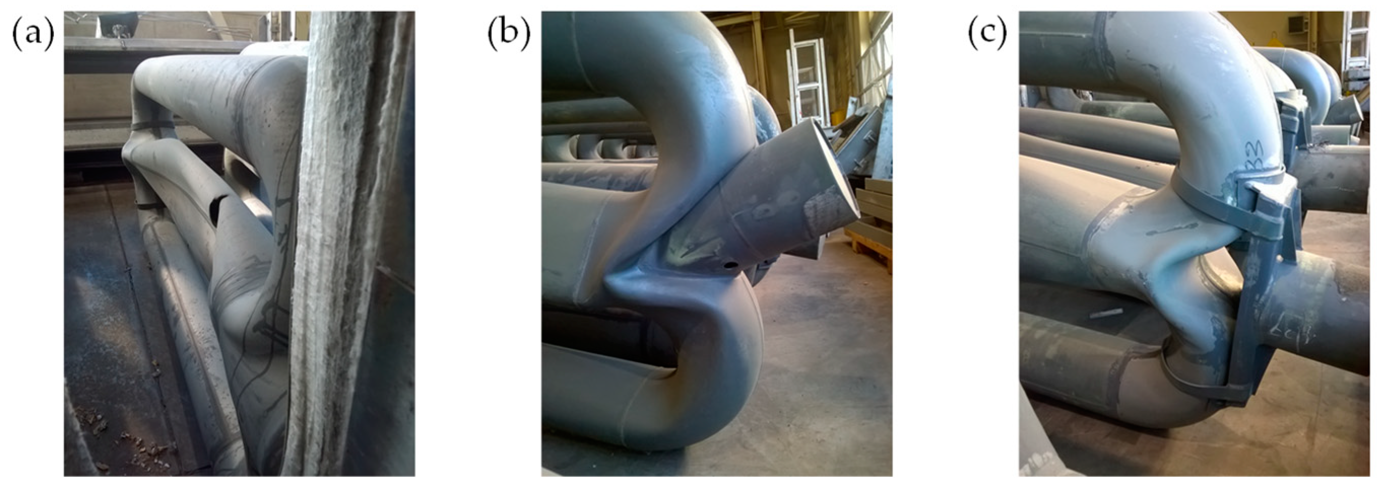
1]. Typical applications include continuous annealing and galvanizing of strip-steel. At high operating temperatures of around 1100 °C, the lifetime of these components is limited by mechanisms such as creep-deformation and material fatigue, causing deformations the tubes [
2,
3,
4]. Examples of damaged double-P-type radiant tubes are shown in
Figure 1.
To maintain product quality with damaged radiant tubes, the productivity (i.e., line speed) must be reduced. Alternatively, damaged radiant tubes need to be replaced, requiring an off-schedule line stop in the worst case [
5,
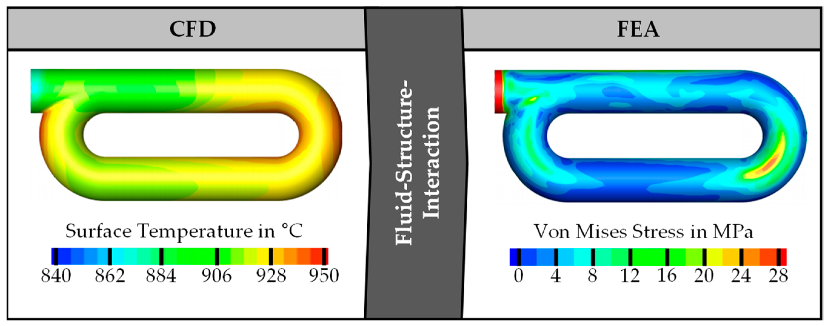
6]. The resulting down times and replacement costs of radiant tubes have led to research focused on predicting radiant tube lifetime in the interest of enabling predictive maintenance measures and adjusting furnace operating parameters to extend radiant tube lifetime. Integral deformation of the tubes over their lifetime can be calculated using fluid-structure-interaction (FSI) approaches, where thermal loads and tube temperatures are calculated in computational-fluid-dynamics (CFD) simulations, which are then transferred into structural finite-element-analysis (FEA) models. This has been applied for W-type radiant tubes by Ifran and Chapman [
7] or Caillat and Pasquinet [
3]. Similar studies were conducted by Hellenkamp et al. [
8], Schmitz et al. [
9], Neumann et al. [
10], or Karthik [
4] for P-type radiant tubes. An exemplary workflow is depicted in
Figure 2. Creep models are employed for the mechanical simulations, with dependencies on quantities such as temperature, the rate of temperature change and thermal stresses induced by temperature gradients in the radiant tubes [
4]. As the creep deformation is directly dependent on the temperature profiles of the radiant tube, CFD simulation results of high accuracy are necessary to obtain a realistic prediction of a radiant tube’s lifetime.
The CFD-model includes the furnace environment, the radiant tube, and major burner components. A Rekumat
® M250 burner [
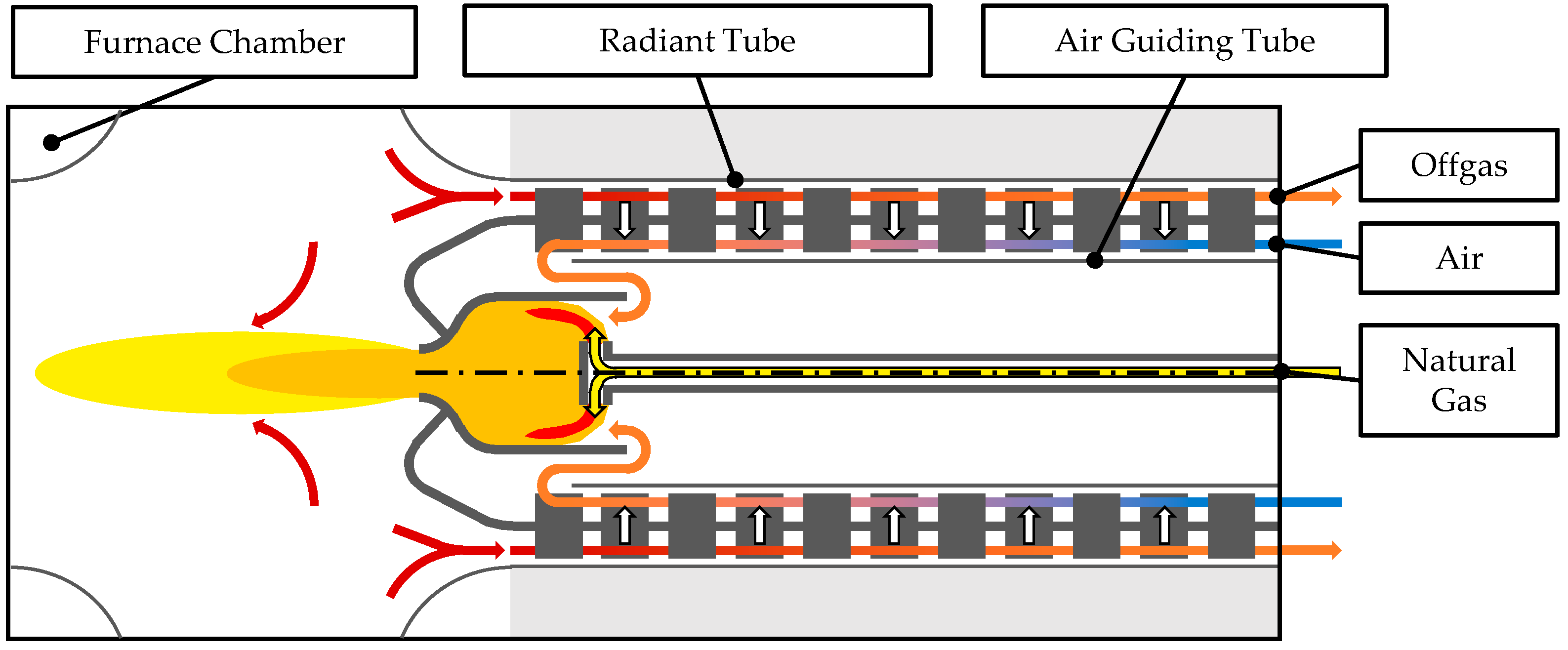
11] id a self-recuperative burner used in recirculating P-type radiant tubes. These burners feature an integrated recuperator to preheat combustion air by transferring heat from the hot combustion products exiting the radiant tube to improve firing efficiency. Recuperators are an example of counter flow pipe heat exchangers (see
Figure 3).
High temperature off-gas is extracted from the radiant tube on the outside of the recuperator, while combustion air enters the system on the inside of the recuperator tube. Guiding tubes are added to the air side to constrain flow to near the surface of the recuperator to enhance heat transfer. On the off-gas side, the temperature of the off-gas flowing through the recuperator directly influences the radiant tubes’ temperature. Fins are added to the recuperator surface, increasing the tubes surface area and additionally inducing turbulence. These effects are paramount for the magnitude of the heat transfer in the recuperator. A high-resolution numerical mesh is needed to accurately model such features in CFD simulations. However, as the simulation models for radiant tube lifetime predictions already feature a complex and computationally expensive setup, using elaborate models for radiation and combustion, general emphasis needs to be put on reducing the complexity of the mesh. Adding a fully detailed recuperator geometry to the model would likely increase the solution time beyond a feasible scope. In past investigations, the recuperator was simplified to a flat tube and the increased heat transfer was not considered [
4,
9]. The section of the tube surrounding the recuperator was neglected in these simulations. The influence of this is visible in the example in
Figure 2. Whereas in reality, the tube is clamped to the furnace wall outside of the system boundaries in this model, the mechanical support in the FEA simulations is defined at the boundary of the modelled section of the radiant tube. This approach results in visible artifacts in the calculated material stresses in the tube, potentially affecting the overall results of the structural simulations.
In order to make the dynamic modelling of recuperators and their surrounding areas of the radiant tube in future numerical investigations feasible, this paper introduces an efficient model to calculate heat transfer and flow inside a fin-typed heat exchanger of a self-recuperative burner. The model is based on the geometrical simplification of the recuperator to a flat tube. This allows for a coarse mesh to be used for the recuperator. Energy transfer and flow patterns are reproduced using specific source terms for the energy and momentum equations. The resulting model can accurately calculate heat transfer and flow patterns inside the recuperator with a significantly smaller mesh for different operating states. This results in a significant reduction in calculation time, without introducing a substantial error compared to a detailed model.
In the following sections, the different CFD models of the recuperator integrated into a Rekumat® M250 self-recuperative burner are being shown. All simulations are performed using the proprietary CFD-software ANSYS® Fluent 2020 R2. First, a detailed simulation featuring the full geometry of the recuperator is discussed. The simulation results are compared against available data sheet specifications. After an evaluation of the simulation results, the simplified model is setup based on the findings of the detailed model. Finally, flow patterns in the simplified model are described and its performance is compared against previous results.
2. Subject of the Models
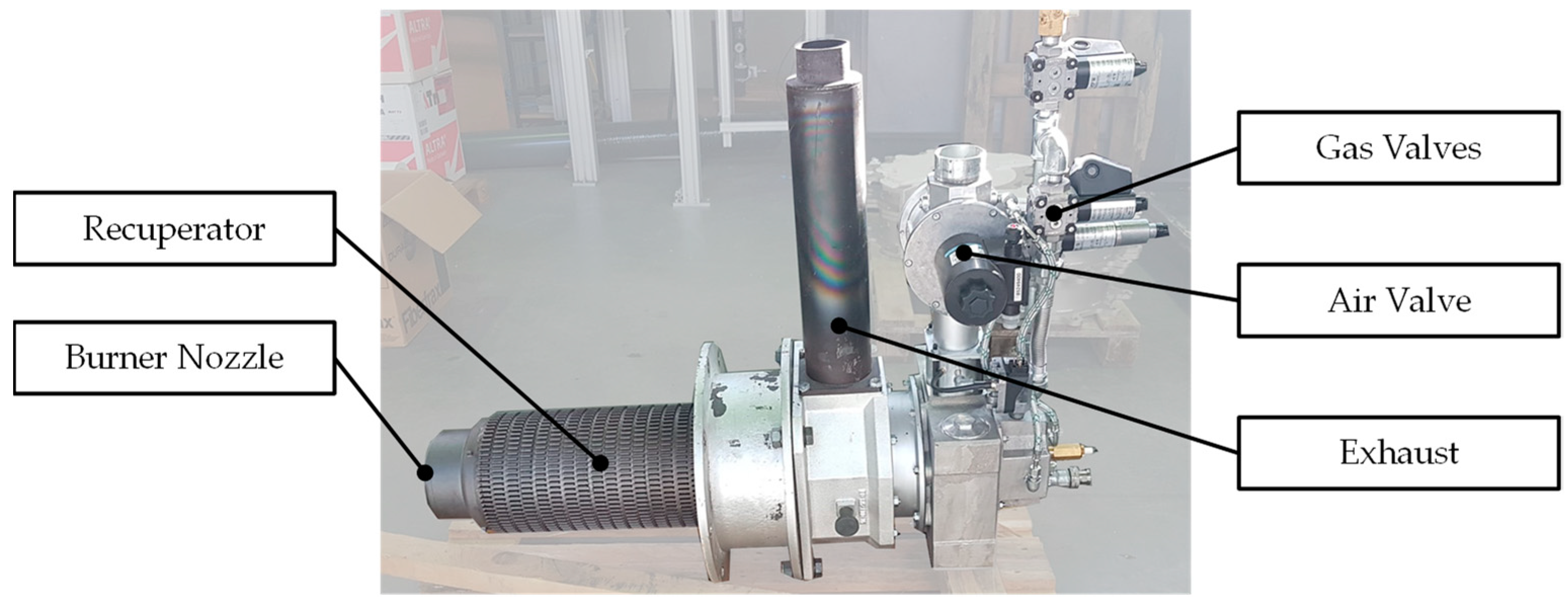
The investigations in this paper are based on the recuperator used in a state-of-the-art, self-recuperative burner. A commercially available variant of the burner is shown in
Figure 4. The Rekumat
® M250 self-recuperative burner is used in direct and indirect fired furnaces and can be operated in conventional combustion and flameless combustion modes. In the investigated configuration, the burner can be operated with power outputs between 120 and 190 kW with a nominal power output of 160 kW. For lower emissions of NOx, the burner can be operated in a flameless combustion mode. To ensure safe combustion, this mode is limited to furnace temperature above 850 °C. The recuperator is made from a heat-resistant casting steel (1.4857). Application temperature of the materials used limit the burners operation to furnace temperatures of up to 1150 °C in direct-fired furnaces [
11].
3. Detailed Model
In the following, the geometry, structure, and results of the detailed CFD model are explained.
3.1. Geometry
The recuperator basic geometry is made up of a finned tube with fins on the inside and outside of the tube. The tube has an inner diameter of 200 mm and a wall thickness of 5 mm. The fins are set up in 20 rows of fins with 72 fins over the circumference of the tube in every row. Consecutive rows are rotated relative to each other by 2.5°. This rotation places the upstream face of a fin in the flow path of the fluid flow between the fins of the downstream row. The fins on the off-gas side are 10 mm tall, while the fins on the air side are taller with 12 mm. The top of the fins is rounded with a diameter of 3.5 mm. The investigated geometry is surrounded by a radiant tube with an inner diameter of 240 mm. A pipe with an outer diameter of 170 mm on the inside of the recuperator is used as a guiding tube for the flow of air. For modelling purposes, the recuperator is extended with a flat tube 100 mm in length, both upstream and downstream, serving as inlet sections to obtain steady velocity profiles by the time the flow reaches the fins. The model’s representation of the recuperator in the simulation is limited to a 20° slice of the geometry to make use of its axial symmetry. The final geometry is shown in
Figure 5.
3.2. Mesh
A polygonal mesh with inflation layers in the fluid zones is created using the meshing tool integrated in ANSYS
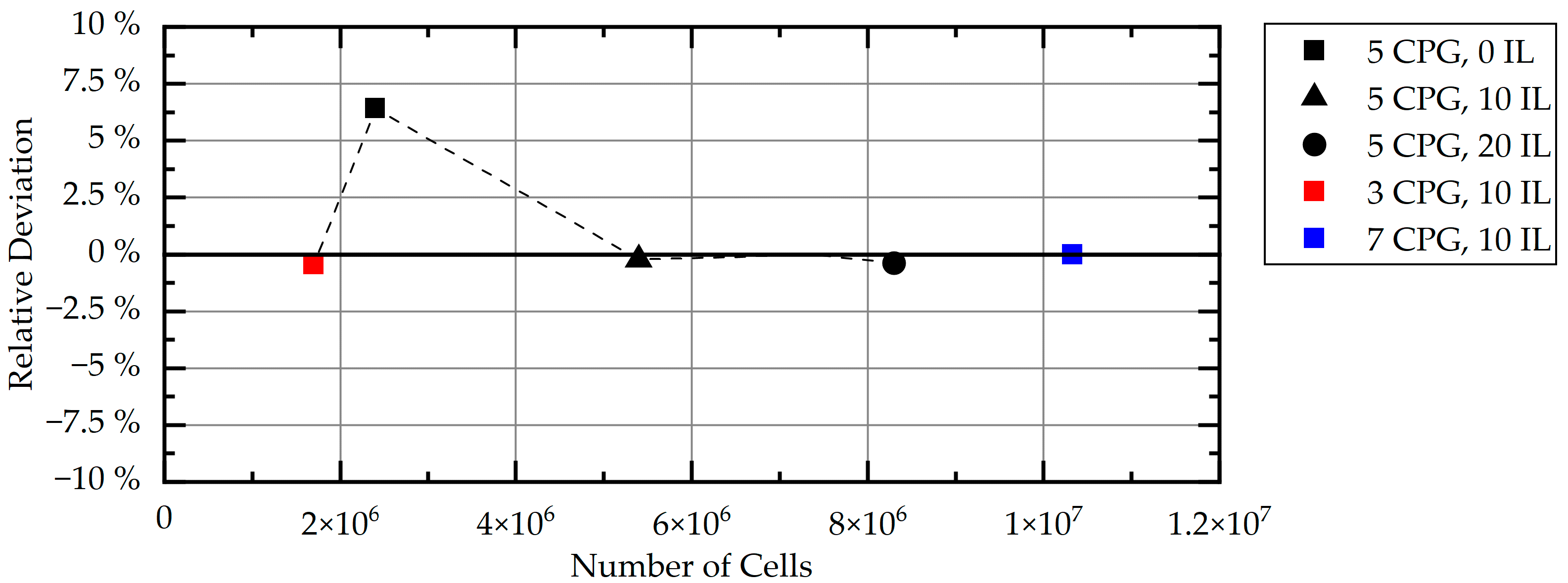
® Fluent. Several different meshes are compared in a mesh study to investigate the dependency of the solution on the mesh resolution. The number of cells per gap (CPG) between edges and faces used to discretize the surface grid is varied, resulting in different cell sizes in the volumetric mesh. Also, the influence of the number of inflation layers (IL) on the wall of the fluid domains was investigated. The heat transfer through the recuperator is used to compare the simulation results. The relative deviation of the different meshes from the simulation with the finest mesh is shown in
Figure 6.
The largest deviation is observed in the mesh variant without inflation layers. A finer boundary layer resolution with 20 cells and seven cells per gap has a negligible influence on the results. Between the mesh variants with ten inflation layers, the deviation from the results achieved with the finest mesh increases with a decrease in mesh resolution. For the study, a mesh with five cells per gap and an inflation layer with ten inflation layers is chosen to ensure sufficient resolution of all flow profiles. The mesh settings applied for all boundary surfaces of a zone in this mesh variant are given in
Table 1. These settings result in a volumetric mesh with 5.2 million cells.
Figure 7 shows the final mesh.
Figure 7a clearly shows the mesh resolution increasing where fins are present without a change in mesh parameters. Cell size in the tube gap is around 2.5 mm and decreases to a cell size of 0.75 mm between the fins. Another significant contribution to the cell count is needed for the meshing of the rounded tops of the fins, where the mesh resolution increases further to around 0.5 mm to capture the radius of the fins. This is evident in
Figure 7b.
3.3. Model Setup
The CFD model is solved for flow, turbulence, energy, radiation, and chemical species. A steady-state, incompressible flow is being assumed. Consequently, Reynolds-averaged Navier-Stokes (RANS) equations may be used. The realizable k-ε-model proposed by Shih et al. [
12] was used to model turbulent effects. The model was chosen primarily to ensure compatibility of the simplified model with simulations of a radiant tube, where the recuperator model will later be integrated. The realizable k-ε-model is often adopted in these models, including combustion mechanics [
4,
13,
14]. Although the boundary layer is resolved with a fine near-wall-mesh in the detailed model, Enhanced Wall Treatment is chosen for a wall-function approach. The definition of wall functions is important for the simplified model, where boundary layers are not resolved by the mesh. The Discrete Ordinates model is used for the modelling of radiation. It is discretized to an angular resolution of 4 × 4 control angles per octant with a pixilation of 3 × 3. With high CO
2 and H
2O fractions, gas radiation is a considerable factor for the heat transfer within the recuperator. The absorption coefficient of gasses is composition- and pressure-dependent. It is calculated using the standard weighted-sum-of-gray-gasses-model (WSGGM), in the simulations. As species concentrations are required for the calculation of the absorption coefficient, transport equations for chemical species are included with the Species Transport model. A 50-species reduced GRI-Mech 3.0 reaction mechanism included in ANSYS
® Fluent is used for the simulations. It is based on the 53-species GRI-Mech 3.0 mechanism, which is a mechanism for the modelling of natural gas combustion [
15]. This mechanism and other reaction mechanisms of similar complexity are frequently used in numerical simulations of natural gas combustion, including radiant tube simulations. Using the same mechanism ensures comparability in the calculation of fluid properties by the chemistry solver between isolated recuperator models and its application in future radiant tube simulation models.
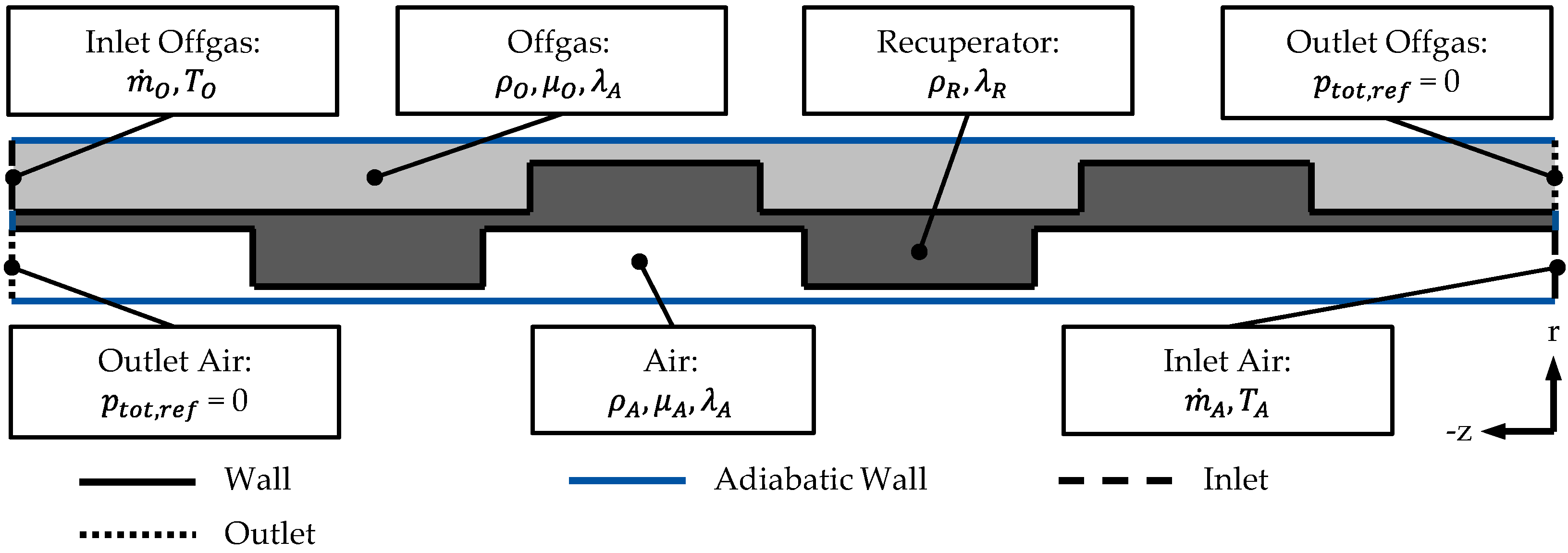
A schematic representation of the model is depicted in
Figure 8. The simulation domain is surrounded by adiabatic walls, inlets, and outlets. The off-gas fluid domain and the air fluid domain are separated by the solid domain of the recuperator. Inlets for the off-gas and air are defined on opposite sides of the model. The radiant tube and air guiding tube are modelled as adiabatic walls. Symmetry boundary conditions are not shown in the schematic, but are defined on the cut planes of the cylindrical section of the recuperator.
The combustion air is defined to enter the domain at a constant composition of 21 vol% O
2 and 79 vol% N
2 and a constant temperature of 30 °C. All other quantities at the inlets are dependent on the investigated operating point. The composition and mass flow rate of the off-gas are dependent on the power input as natural gas and air-fuel ratio (AFR) of the burner. AFRs above one are primarily investigated, as they are primarily used in radiant tubes to ensure complete combustion and consequently, low emissions [
16]. The off-gas temperature varies on the operating conditions of the furnace the burner is operated in and is varied between 850 °C and 1150 °C, limited by the operating range of the burner.
Table 2 shows the values for mass flow rates and off-gas composition for several burner power settings and AFRs. The operating point at 160 kW, with an AFR of 1.15 is used as a baseline scenario. The values were calculated from the combustion of a gas mixture with 95% CH
4 and 5% C
2H
6. Reactions are not modelled in the simulation. The combustion is assumed to be completed by the time the off-gas enters the recuperator boundaries. Thus, species concentrations are constant on both sides of the recuperator and are defined only by the respective species concentrations defined at the fluid inlets.
Material properties for 1.4857 are listed in
Table 3. Density and specific heat are constants, while the thermal conductivity is linearly interpolated for temperature between the given points. Material properties for the fluids are dynamically calculated dependent on gas composition and temperature. The density of the fluid mixtures is calculated as an incompressible ideal gas. Specific heat, thermal conductivity, viscosity, and mass diffusivity are calculated by the integrated ANSYS
® Chemkin CFD-Solver. Sampled of fluid properties calculated in the solver in comparison with values available in literature are given in
Appendix A (see
Figure A1,
Figure A2,
Figure A3 and
Figure A4). Default ANSYS
® Fluent 2020 R2 settings were retained for all model settings and boundary conditions not specifically described in this section.
3.4. Results
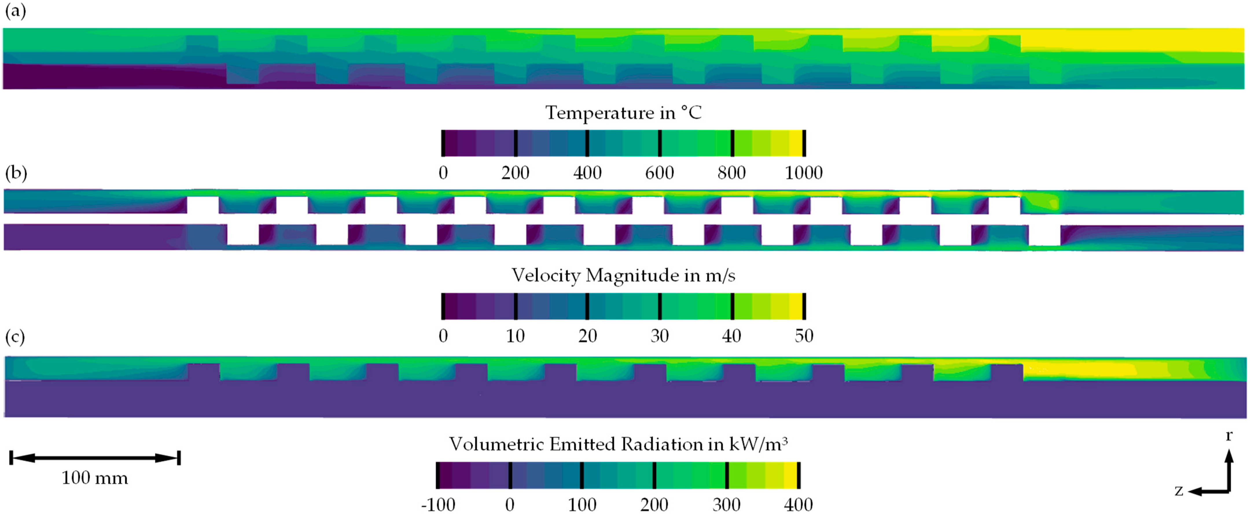
The results of the detailed simulation model are shown in
Figure 9 for the baseline scenario. The off-gas temperature decreases from 1000 °C at the inlet to 625 °C at the outlet. The air temperature is increased from 30 °C at the inlet to 524 °C at the outlet. The amount of air preheat achieved in heat exchangers can be described by the relative air preheat [
1], according to Equations (1) and (2).
is the temperature of the air entering the heat exchanger,
is the air temperature at the outlet of the heat exchanger, and
is the temperature of the combustion gasses entering the recuperator. The relative air preheat in the investigated operating point equates to 0.52, which is within the characteristic range for self-recuperative burners [
18]. A total of 1847 W is transferred from the off-gas to the combustion air. Part of the fluid flows through the gap between the top of the rounded fins and the guiding tube with a higher fluid velocity then the fluid flowing through the fins. The influence of gas radiation is relevant on the off-gas side of the recuperator, visible in
Figure 9c. Radiation is not emitted or absorbed by the combustion air. A total of 510 W of radiation is absorbed by the recuperator wall from the off-gas fluid domain, equivalent to 27.5% of the total heat transfer. In a simulation setup neglecting radiation, heat transfer is reduced by 19% to 1496 W.
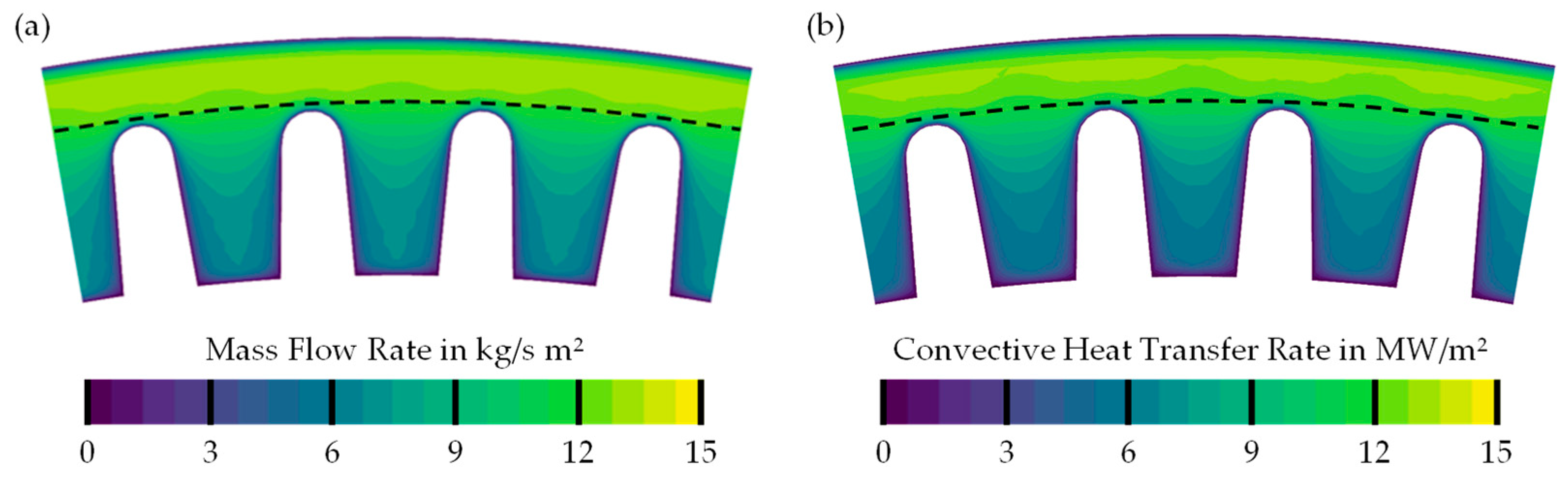
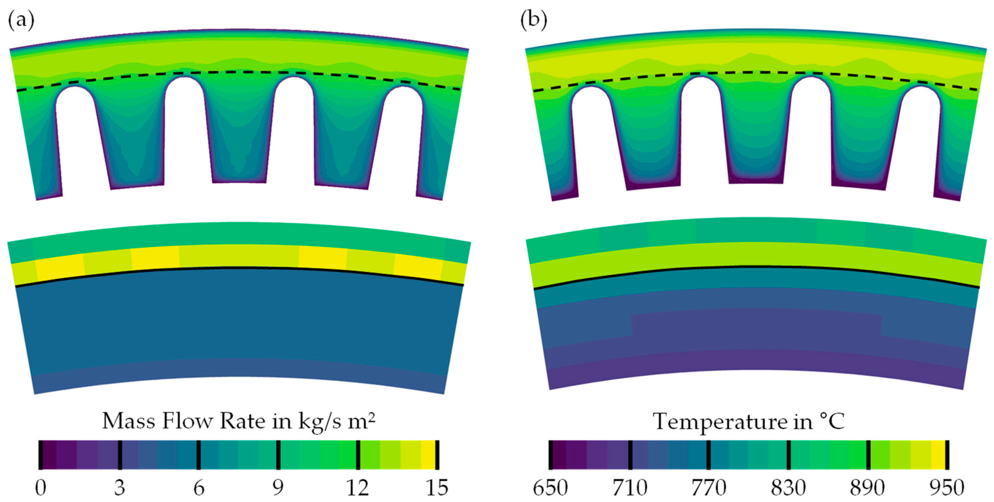
Figure 10a shows the area normalized mass flow rate through a radial cross section of the off-gas fluid volume. A dashed line separates the cross section into two areas of equal mass flow.
The area above the dashed line represents 40% of the total cross-sectional area. A total of 52% of total mass flow is flowing through this cross-section. A temperature difference of around 100 °C is observed between the off-gas flowing through the gap and off-gas flowing through the fins. This temperature difference induces an equally uneven distribution of convective heat transfer rate through the gap (s.
Figure 10b), which represents 64% of total convective heat transfer. Without being in direct contact with the fins and therefore not in direct heat exchange with the recuperator, the gap flow reduces the efficiency of the recuperator. The representation of the gap flow is a priority for the simplified model. Flow patterns on the air side show similar effects. However, as the off-gas flow is in direct contact with the radiant tube, this investigation focusses primarily on the flow patterns on the off-gas side.
In-situ measurements of the recuperator for the purpose of validation of the model were not performed. Instead,
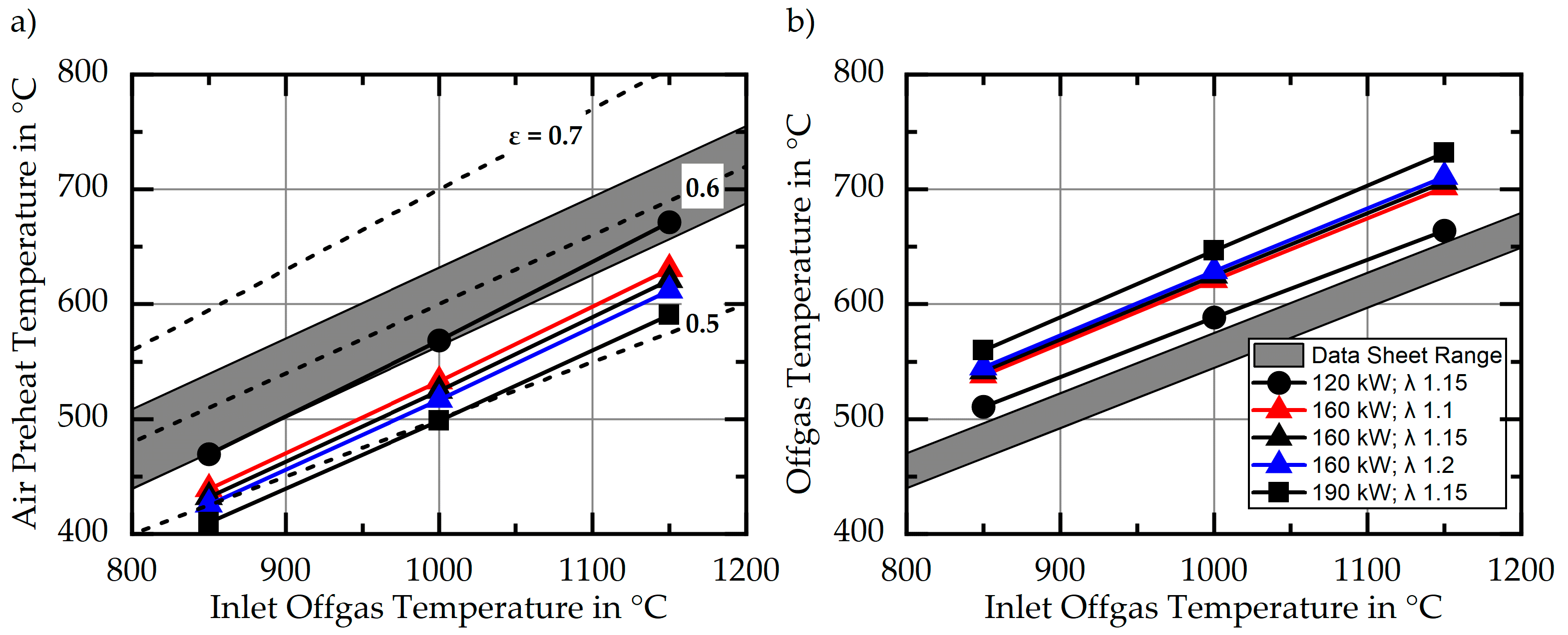
Figure 11 shows the air preheat temperature and off-gas temperature in comparison with data sheet values. Air preheat temperatures are below the data sheet range in most operating points. The correlation improves for lower burner power outputs and lower AFRs. The results are the closest to the data sheet range at the lowest power output of 120 kW and an AFR of 1.1. Higher mass flow rates at higher burner power outputs and higher AFRs result in lower air preheat temperatures. Although not shown in the diagram for legibility, the change in air preheat temperature between different AFRs is comparable for all power outputs of the burner. Relative air preheat is in the range of 0.5 to 0.6, which is within the characteristic range for self-recuperative burners [
18]. In accordance with these results, off-gas temperatures at the recuperator outlet are higher than data sheet figures. The temperature spread between operating points is lower for the off-gas temperatures than the air preheat temperatures. This is attributable to the higher specific heat capacity of the higher temperature off-gas compared to that of the air.
Operating conditions and testing methodology under which the burner was tested to obtain the given values in the data sheet are not given in the documentation. Therefore, the given temperatures may not necessarily be suitable for the validation of the simulation. Differences might arise, for example, from measurement positions different to the model boundaries, differences in boundary conditions such as air temperature. Nevertheless, the simulations coincide with the data sheet specifications at lower burner power settings. The gradient of air preheat and off-gas temperature with changes in the inlet off-gas temperature are also in good agreement with the data sheet specifications. Therefore, it is assumed that major flow features are calculated with sufficient accuracy to serve as a basis for the development of a simplified model. In the following sections, this study focusses on evaluating the error introduced by the modelling approach presented instead of assessing the agreement of the simulation results with measurement data from a recuperator or matching simulation results to data sheet specifications.
4. Simplified Model
In this section, the simplified recuperator model is introduced. It is based on the geometric simplification of the recuperator to a flat tube. This results in the loss of geometrical information, which allows for a significantly coarser mesh to be used. To compensate for neglecting parts of the geometry, different source terms for pressure loss and energy are being used to replicate the flow field and temperature field from the detailed model introduced in the previous section. The model assumes evenly distributed heat transfer and pressure loss in the region throughout the finned region of the recuperator. The momentum source terms are dependent on the velocity magnitude of the flow and fluid properties. The heat transfer is only modelled based on a temperature difference between a solid body and a surrounding fluid. Influences of turbulent quantities on the heat transfer are not modelled. The errors, introduced by the simplifications made, are evaluated by comparison with the results from the detailed model.
4.1. Geometry and Mesh
A structured hexagonal mesh is created for the simplified geometry of the recuperator. For the fluid domains, cell size in the radial direction is 2 and 5 mm in the axial direction. This resolution resolves the gap between the top of the fins and the guiding tubes with two cells across the gap. Angular resolution is one cell per degree of circumference. A mesh study is not performed, as the heat transferred through the recuperator is primarily influenced by parameters set in the custom source terms used to model heat transfer. The mesh settings result in a volumetric mesh with 80,902 cells, which corresponds to a reduction in mesh size of 98.5% compared to the detailed model. The simplified geometry and the resulting mesh are shown in
Figure 12.
4.2. Simplified Modelling Approach
Like the detailed model, fluid domains are defined for the off-gas (Index
) and the air side (Index
). A cross section of the model is depicted in
Figure 13. Separate fluid domains are defined for the fin regions (hatched areas in
Figure 11). Two different source terms are defined in these domains: A momentum source term to account for the pressure loss caused by the fins (
) and an energy source term to calculate the increased energy transfer through the fins (
). The pressure loss term from the Porous Media Model available in ANSYS
® Fluent Porous Media Model is used to model the pressure loss, as homogenous pressure loss is assumed. The corresponding domains are named porous media. Source terms from the model are implemented using custom momentum source terms. This is the first part of the simplified model.
Those porous media domains (hatched areas in
Figure 11) and the section of the tube in between these are copied onto the same location, adding the second part of the model. This second part represents the solid part of the fins and is used to model energy transfer between the off-gas side and air side of the recuperator through thermal conduction. It has no interaction with any flow quantity in the fluid domain other than the user-defined energy source terms. The two model parts are coupled using the additional energy source term
, defined in the middle section of the recuperator wall, both in the solid and the fluid part.
To model the gap flow observed in the detailed simulations, a non-permeable two-dimensional surface is added on the circumferential surface of the porous medium. Without this wall, strong velocity gradients exist between the flow through the gap and the flow through the porous media exist. Turbulence induced by these gradients smooths out the gap flow and reduced its influence on the overall flow and energy fields in the recuperator. A constant wall shear stress of zero is defined on this surface to prevent an influence on pressure loss. The wall is also defined as transparent to radiation with a diffuse fraction of zero. Other settings for the simplified model, such as the parameters for the inlets and outlets or adiabatic walls, as well as the equations solved are identical to the setup presented in
Section 3. The closing source terms and their derivations are described in the following subsection. The source files for all custom source terms and functions are provided in the
supplementary materials.
4.2.1. Pressure Loss
Pressure loss source terms are added to the model in the porous media domains to account for the pressure loss introduced by the physical presence of the fins. The pressure loss also results in the existence of the pronounced gap flow. The pressure loss is assumed to be uniform. It is modelled using a common approach for modelling the pressure loss in porous media. The pressure loss caused by a flow in direction
of a cartesian coordinate system is described by Equation (2) [
19].
and
are prescribed resistance matrices. In homogenous porous media, both matrices can be simplified to diagonal matrices. The values on the diagonal
and
are referred to as the inverse permeability and the inertial resistance factor in direction
.
is the velocity magnitude of the flow. Circumferential flow is largely inhibited by the fins, since the design of and the flow through the recuperator are such that no significant radial components (except locally very close to individual fins) are generated during the flow. In the simplified modeled, this can be assured by using a large pressure loss term for the radial velocity. In practice however, such pressure loss terms for the circumferential flow may lead to convergence issues. As there are no geometrical features inducing radial flow components in this simplified model, no additional radial pressure loss terms will be used. The source term in the axial direction is simplified to a term dependent on two geometry dependent variables, resulting in Equation (3) [
19].
The pressure loss in a porous medium with a given thickness of
can be given by Equation (4) [
19].
Values for
and
are obtained by calculating the pressure loss in the detailed model for several flow velocities and fitting the resulting function according to Equation (5) [
19].
A comparison of Equations (4) and (5) results in Equation (6) for the calculation of the variables for the pressure loss term [
19].
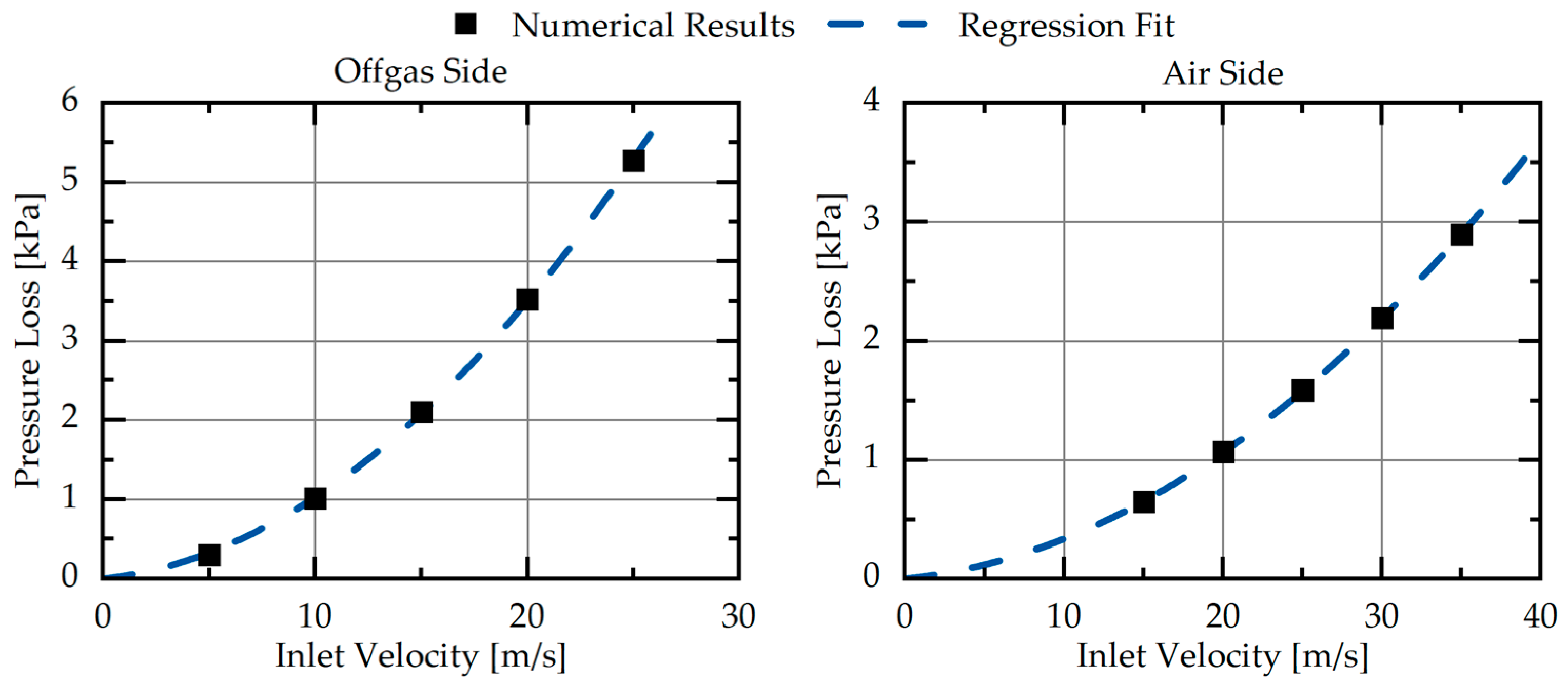
Sample points for pressure loss to create a second-degree fitting function corresponding to Equation (5) are extracted from results of a reduced version of the detailed model. Here, the detailed model is modified, as the variables are influenced by the temperature-dependent quantities of
and
. To eliminate a change in these quantities, pressure loss is evaluated in an isothermal flow. The pressure loss is calculated as the difference in total pressure between a plane at the start of the fins and the end of the fins in the direction of the flow, depending on the inlet velocity. The inlet velocities used are based on average velocities observed in the detailed simulation results. The resulting regression fit Equations (7) and (8) are a perfect fit for the observed pressure loss. The results for the off-gas and the air domain are given in
Figure 14.
The inputs for Equation (6) and the resulting values for
and
are given in
Table 4. These results are implemented into the momentum source terms in the model.
4.2.2. Heat Transfer
The source terms for heat transfer
in the recuperator are based on a basic equation for convective heat transfer, Equation (9).
is the local heat transfer coefficient.
refers to a local temperature difference between a surface and a surrounding fluid. Instead of the total surface area, the term is defined with the specific surface area
, to obtain a volume specific formulation for the source term, Equation (10).
is the volume of the fluid domain, where the source term is defined (here: porous media domains in the off-gas or air region) and
is the surface area of the fins in this area of the volume region in the detailed geometry. Average values for the heat transfer coefficient on the off-gas side (Index
,
) and the air-side of the recuperator (Index
,
) are obtained from the results of the detailed simulation for the reference operating point. Values for the specific surface areas and the heat transfer coefficients in the baseline scenario are given in
Table 5.
However, the calculation of a heat transfer coefficient in the sense of Equation (9) requires the definition of a free stream temperature. This temperature is dependent on the location where the heat transfer is evaluated and is not easily defined in a complex geometry such as the recuperator. Consequently, using the calculated values for the heat transfer coefficient in the simplified model does not yield results matching the heat transfer in the detailed model. Instead, the value of the heat transfer coefficient in the source terms is iteratively optimized to match the heat transfer in the simplified model with the heat transfer in the detailed model. To reduce the iterative process to the changing of
as a single variable, the factor
, Equation (11), is introduced as the ratio of the heat transfer coefficients between the sides.
Using the values from
Table 5 gives a value for
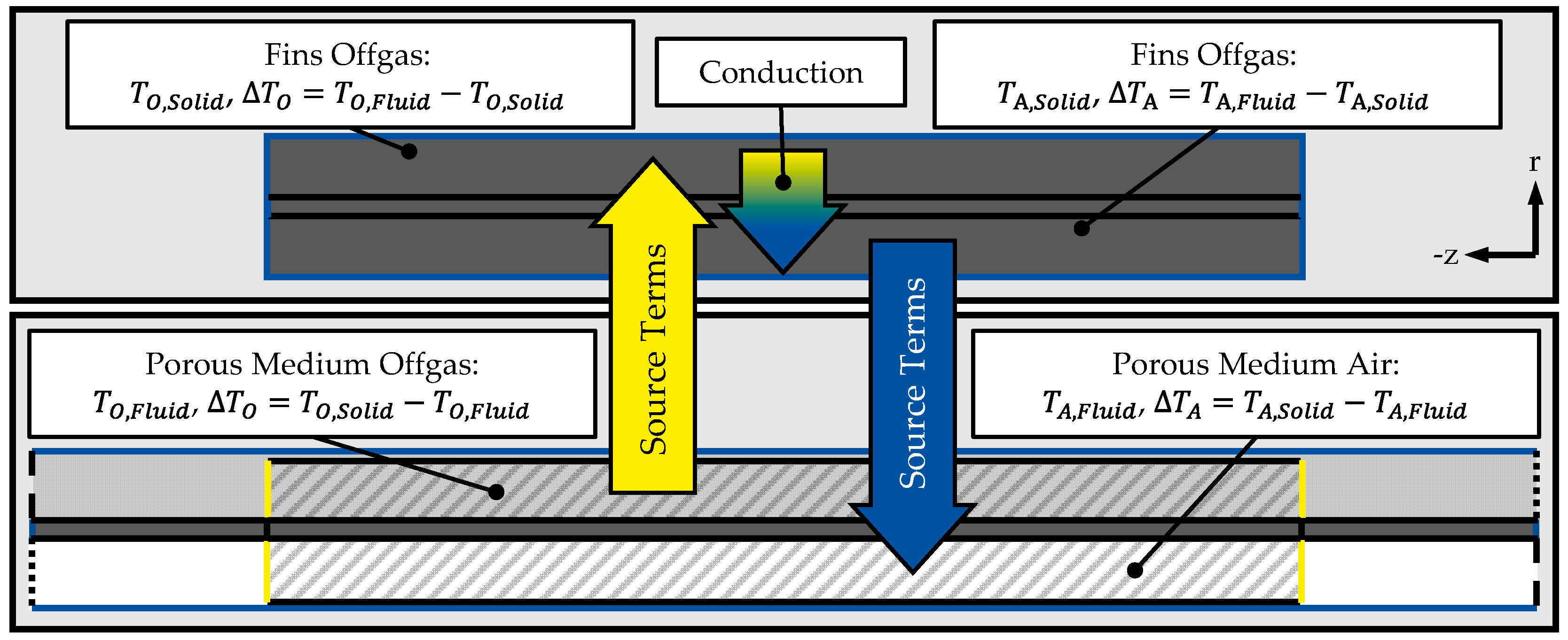
. The source terms for the off-gas and air side are then defined with Equations (12) and (13). These source terms are defined in the fluid and solid domain in both the air and off-gas regions of the model. The definition of the temperature difference depends on where the source term is defined. Thus, the resulting energy balance is kept valid.
The source terms are defined in the fluid and solid domain in both regions of the model. The definition of the temperature difference depends on where the source term is defined. Thus, the resulting energy balance is kept valid. The corresponding temperature difference terms and the resulting energy flows are illustrated in
Figure 15.
A third energy source term is defined in the recuperator walls. Since these volume bodies are essentially representing the same component in both parts of the model, their energy source term is setup to average out possible temperature differences, Equation (14).
T factor
is introduced to create an underrelaxation to the terms and help convergence of the model. Here, it is set to a value of 0.4. All energy source terms require getting the temperature from the identical cell in the overlaying cell zone before the calculation can commence. For this purpose, a matching function is defined, which, for every cell, performs a nearest-neighbor search for the cell at the identical position in the overlaying cell zone and stores the reference to this cell in the memory. A temperature exchange function using this reference evaluates the temperature of the overlaying cell when the source terms are calculated. The coupling functions are defined in the source files provided as
supplementary material.
As stated previously, the energy transfer in the simplified model is matched to the results of the detailed model by iteratively changing the value for . The energy transfer of the detailed model is matched with the simplified model with a value of = 159.8 W/m²K. By adapting this parameter, the model can be adjusted to achieve any desired heat transfer or air preheat values. Hypothetically, the model could be adjusted to match the data sheet specifications exactly, if desired. However, this study focusses on the quality of the result replication from the detailed model using the described simplified model.
5. Simplification Results
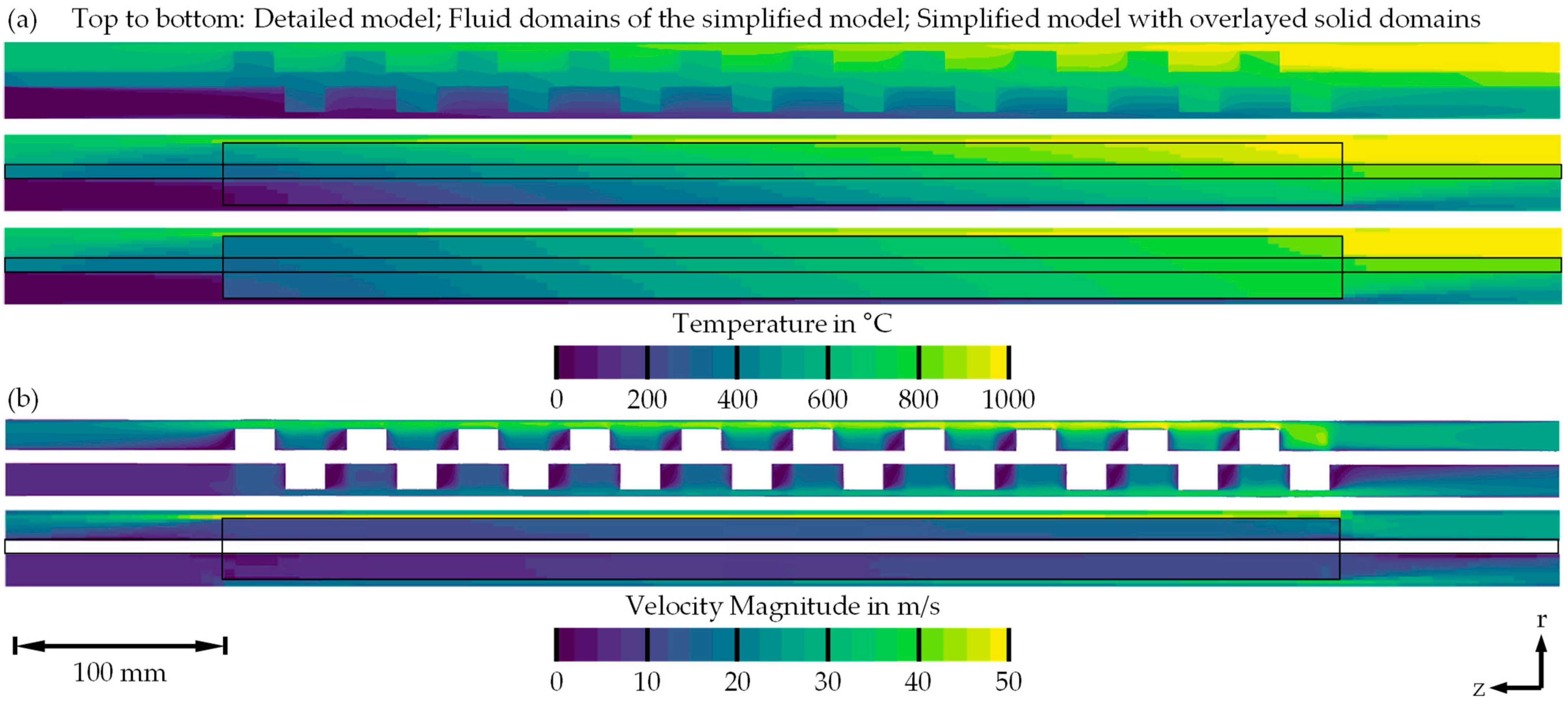
Figure 16 shows fluid velocity and temperature on an axial cross-section in comparison between the detailed and simplified model for the baseline scenario. A high agreement of the models can be observed in the temperature profiles. Both the fluids in the porous zones, as well as the overlaying solid zones show similar profiles and gradients to their counterparts in the detailed model. The temperature difference between the flow through the porous media and the flow through the described gap is higher in the detailed model, then in the detailed model. As the heat transfer is matched for the operating point shown, heat transfer and air preheat temperatures are equal in both cases. The velocity plot
Figure 16b shows more steady velocity profiles, and generally lower velocity magnitudes in the porous media resulting from larger cross-sectional areas for the flow without the inclusion of the fins.
Figure 17 shows fluid velocity and temperature in radial cross sections of the off-gas domain at
= 340 mm for the detailed and simplified models. The normalized mass flow rate is significantly lower in the simplified model. However, integral distribution of the gap mass flow is nearly equal for both cases, with 52.74 and 51.97% of total mass flow in the detailed and simplified model, respectively. Similar relationships can be observed for the temperature. The total temperature is decreased in the flow through the porous media in the simplified model above 50 °C. Nevertheless, the total convective heat transfer rate again shows good agreement with 54.67%, and 57.64% of total convective heat transfer being transported through the gap for the detailed and simplified model respectively.
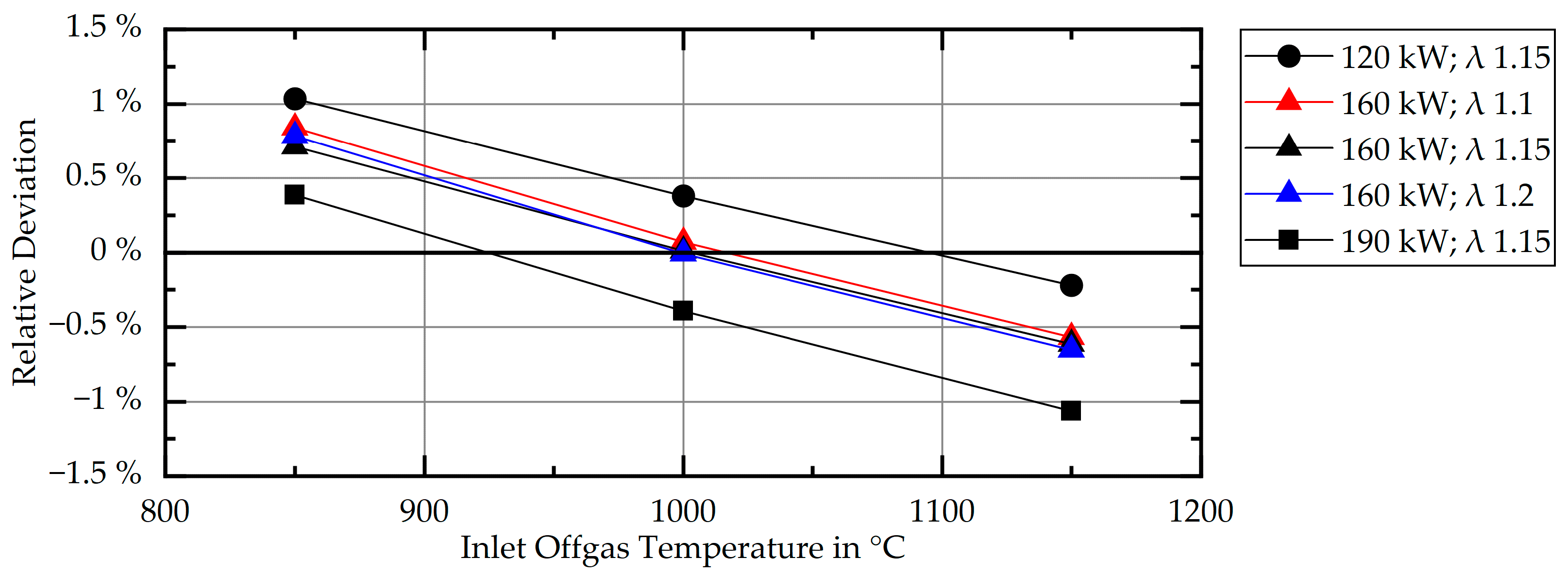
To evaluate the model’s performance with changes in operating parameters, the relative deviation of the simplified models results from those of the detailed model is shown in
Figure 18 for several operating points. The relative deviation
is described by Equation (15).
is the net heat transferred from the off-gas to the air. Heat transfer in the detailed model deviates by a maximum of 1.2% across all operating points investigated in this study. Off-gas temperature at the recuperator inlet generally shows a bigger influence on the deviation then differences in mass flow rates or species concentrations with the different operating points.
Over the investigated range in off-gas temperature at the inlet of 300 °C, the deviation decreases by 1.3% on average. With the variation of burner power, the deviation is within a range of 0.8% at the maximum temperature of 1150 °C. The deviation decreases with lower temperatures. Changes in AFR have a negligible effect on the model’s accuracy. At an off-gas temperature of 1000 °C and a burner power output of 160 kW, the deviation varies between 0.07% for λ 1.1 and −0.01% for λ 1.2. Hence, if the model is adapted to a specific operating condition, the heat transfer of the simplified and the detailed model are almost identical, even with slight changes in AFR or off-gas temperature at the inlet.
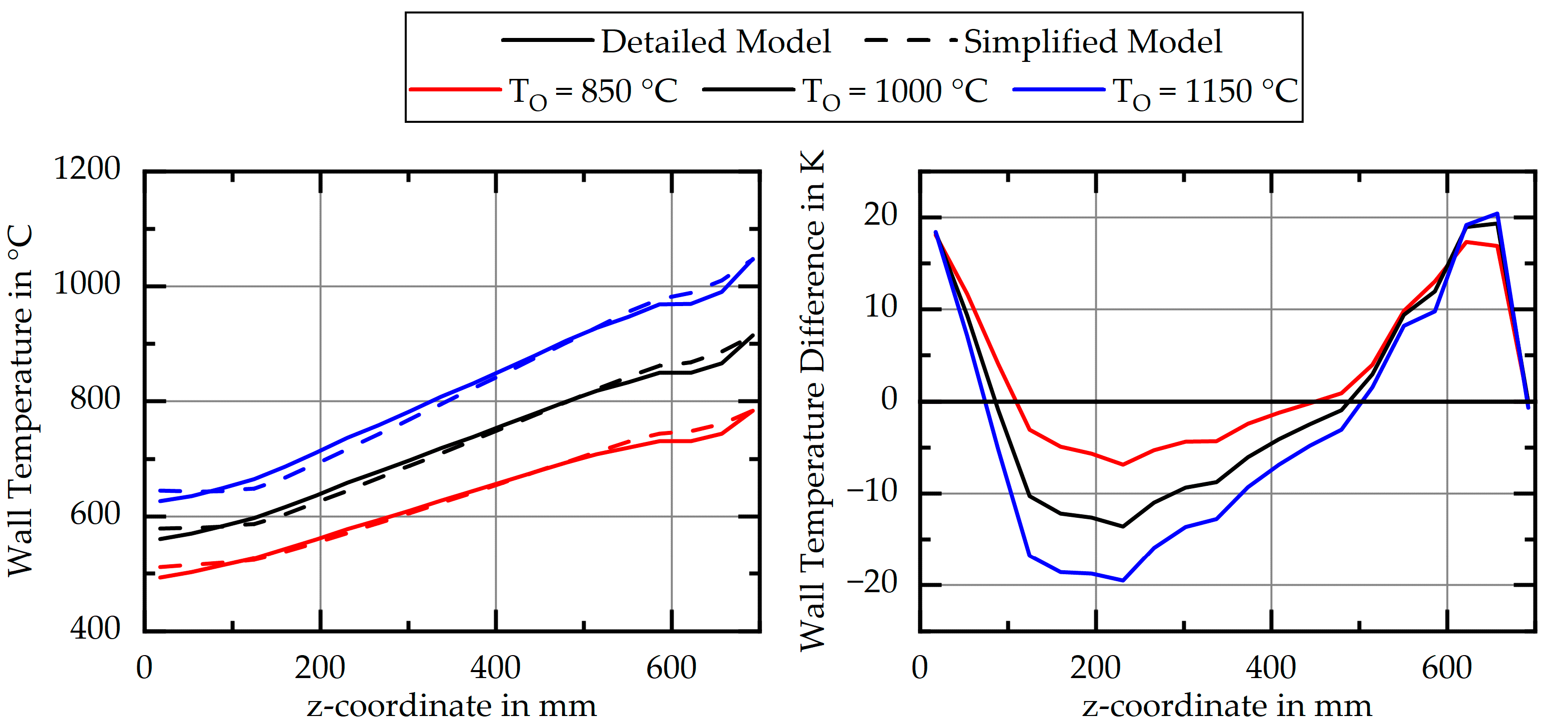
One aim of the model was to dynamically calculate the temperature of the surrounding radiant tube. Average wall temperature of the surrounding tube in both models is shown in
Figure 19. The deviation in wall temperature between the models varies with the axial position. Near the off-gas inlet, temperatures in the simplified model are up to 10 K higher for all off-gas inlet temperatures. Further downstream, lower temperatures are calculated in the simplified model. The deviation depends on the inlet’s off-gas temperature with a maximum of around 20 °C for an off-gas temperature of 1150 °C. A higher agreement is achieved for lower temperatures at the inlet, with a maximum of 7 °C for an off-gas inlet temperature of 850 °C. Close to the off-gas outlet, the deviation increases again to a maximum of 18 °C for all off-gas inlet temperatures. Notably, the deviation is not minimal for the design operating point. As the error decreases with temperature, it can be assumed that it is related to a wrong radiation heat transfer calculation due to the geometry reduction.
6. Summary
The presented paper introduces an approach of efficiently model heat transfer and flow patterns in a fin-type heat exchanger in self-recuperative burners. Overall, the simplified model reproduced heat transfer in the detailed model with a maximum deviation of around 1% for a large set of operating points, while simultaneously reducing the necessary mesh size by 98.5%. The flow patterns inside the recuperator itself are showing significant differences between the models, which is a result of the geometrical simplifications. However, results for heat transfer, air preheat, wall temperatures, and flow distribution are in very good agreement with each other. This deviation can be decreased to almost zero, if the model is designed for a specific operating point, characterized by the off-gas temperature at the inlet and the burner power.
While the presented model is specific to the Rekumat® M250 burner, expansions are conceivable to replicate recuperators in similar burners. The model can easily be adapted by following the same workflow of first creating a detailed model of the recuperator and subsequently adjusting the simplified model’s geometry, mesh, and parameters to the recuperator of interest. This also includes expansion of the model to new recuperator types like nubbed or burled recuperators. In these cases, the modelling approach must be adjusted to changes in flow phenomena, which are specific to that type of recuperator. However, the model’s accuracy might vary for every new application and thus must be evaluated separately for every new recuperator modeled.
In the future, investigation of the model’s behavior in transient simulations is of interest especially for FSI-simulations of radiant tubes. Furthermore, the model can be expanded with new parts such as thin or insulated off-gas guiding tubes separating the flow inside the recuperator from the radiant tube. Most importantly, the behavior of the model inside a radiant tube simulation needs to be investigated. Particularly, it is not clear how the temperature and radiation inside the radiant tube will have an effect on the heat transfer inside the recuperator.
Author Contributions
Conceptualization, N.D., N.S., C.S. and H.P.; Investigation, N.D.; Resources, N.S. and H.P.; Supervision, N.S., C.S. and H.P.; Visualization, N.D.; Writing—original draft, N.D.; Writing—review and editing, N.D., N.S., C.S. and H.P. All authors have read and agreed to the published version of the manuscript.
Funding
This research received no external funding.
Conflicts of Interest
The authors declare no conflict of interest. The funders had no role in the design of the study, in the collection, analyses, or interpretation of data; in the writing of the manuscript, or in the decision to publish the results.
Appendix A
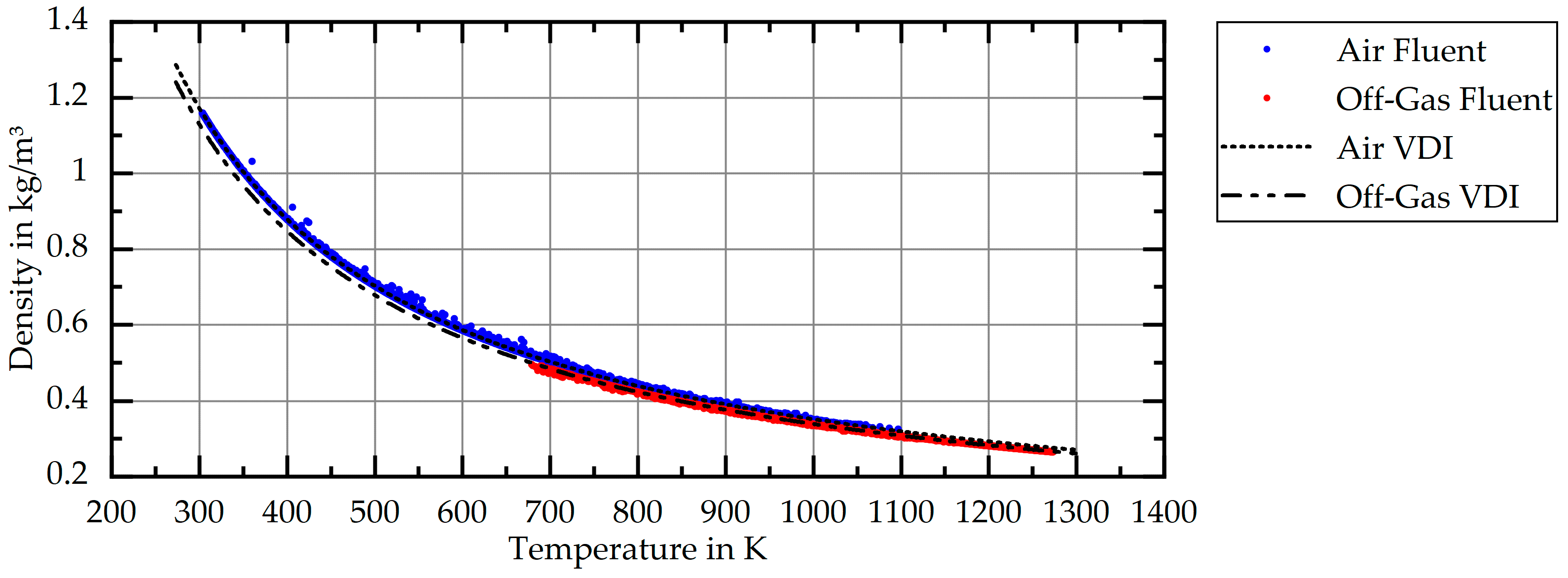
Figure A1.
Sampled data points of the fluid density of air and off-gas at λ = 1.15 calculated in ANSYS
® Fluent in comparison with values calculated with methods described in [
20].
Figure A1.
Sampled data points of the fluid density of air and off-gas at λ = 1.15 calculated in ANSYS
® Fluent in comparison with values calculated with methods described in [
20].
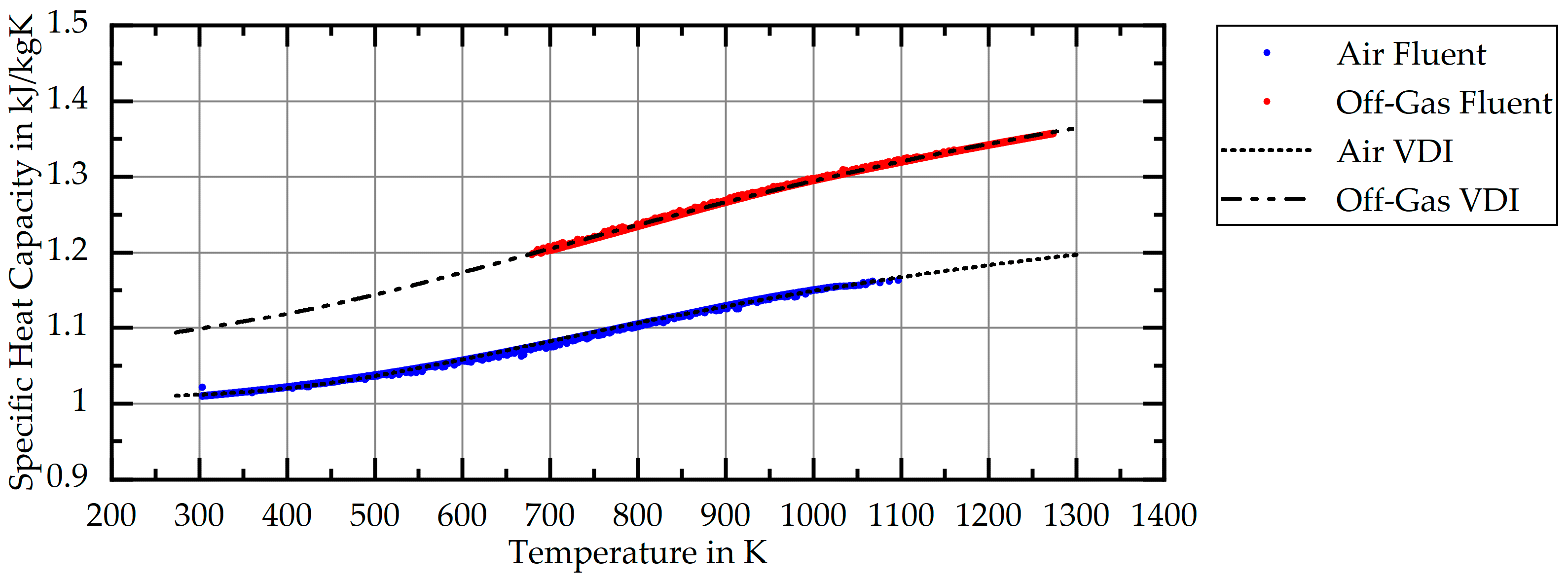
Figure A2.
Sampled data points of the specific heat capacity of air and off-gas at λ = 1.15 calculated in ANSYS
® Fluent in comparison with values calculated with methods described in [
20].
Figure A2.
Sampled data points of the specific heat capacity of air and off-gas at λ = 1.15 calculated in ANSYS
® Fluent in comparison with values calculated with methods described in [
20].
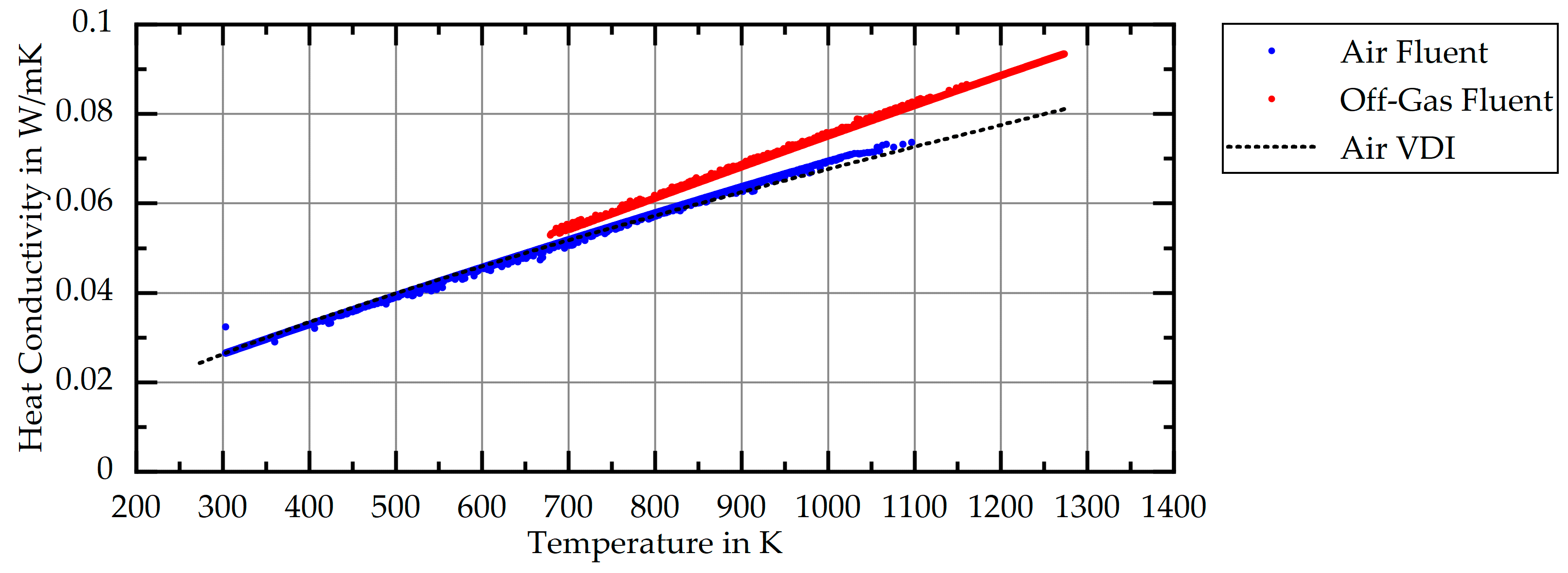
Figure A3.
Sampled data points of the heat conductivity of air and off-gas at λ = 1.15 calculated in ANSYS
® Fluent in comparison with values from [
21].
Figure A3.
Sampled data points of the heat conductivity of air and off-gas at λ = 1.15 calculated in ANSYS
® Fluent in comparison with values from [
21].
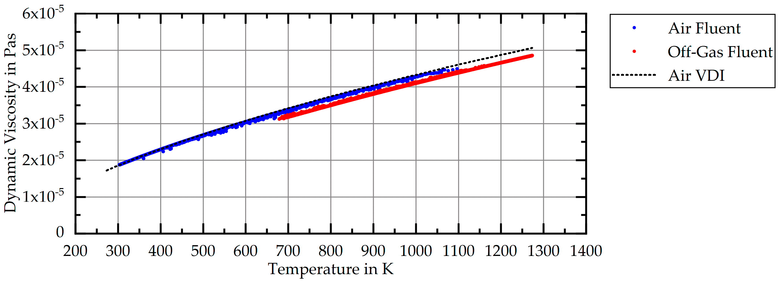
Figure A4.
Sampled data points of the dynamic viscosity of air and off-gas at λ = 1.15 calculated in ANSYS
® Fluent in comparison with values from [
21].
Figure A4.
Sampled data points of the dynamic viscosity of air and off-gas at λ = 1.15 calculated in ANSYS
® Fluent in comparison with values from [
21].
References
- Beneke, F.; Nacke, B.; Pfeifer, H. (Eds.) Handbook of Thermoprocessing Technologies: Volume 2: Plants, Components, Safety; Vulkan-Verlag GmbH: Essen, Germany, 2015; ISBN 3802729765. [Google Scholar]
- Büschgens, D.; Karthik, N.K.; Schubert, C.; Schmitz, N.; Pfeifer, H. Investigation of the Influence of Proximal Radiation on the Thermal Stresses and Lifetime of Metallic Radiant Tubes in Radiation-Dominated Industrial Furnaces*. HTM J. Heat Treat. Mater. 2019, 74, 392–405. [Google Scholar] [CrossRef]
- Caillat, S.; Pasquinet, C. Radiant tubes lifetime prediction in steel processing lines using fluid—Structure interaction modelling. Energy Procedia 2017, 120, 596–603. [Google Scholar] [CrossRef]
- Karthik, N.K. Investigations on the Effects of Alternating Temperatures on the Lifetime of P-Type Radiant Tubes; SCL Verlag: Aachen, Germany, 2020. [Google Scholar]
- Schmitz, N.; Karthik, N.; Pfeifer, H.; Wuenning, J.G. Durability of metallic radiant tubes in galvanizing lines. In Proceedings of the 111th Annual Meeting of the Galvanizers Association, Charleston, SC, USA, 15 October 2019. [Google Scholar]
- Wünning, J.G. Factors, Influencing Radiant Tube Life. In Proceedings of the 106th Meeting of the Galvanizers Association, Jackson, MS, USA, 5–8 October 2014. [Google Scholar]
- Irfan, M.; Chapman, W. Thermal stresses in radiant tubes: A comparison between recuperative and regenerative systems. Appl. Therm. Eng. 2010, 30, 196–200. [Google Scholar] [CrossRef]
- Hellenkamp, M.; Pfeifer, H. Thermally induced stresses on radiant heating tubes including the effect of fluid–structure interaction. Appl. Therm. Eng. 2016, 94, 364–374. [Google Scholar] [CrossRef]
- Schmitz, N.; Schwotzer, C.; Pfeifer, H. Increasing lifetime of metallic recirculating radiant tubes. Heat Process. 2018, 16, 49–55. [Google Scholar]
- Neumann, A.; Brykarczyk, D.; Lenz, W.; Bambach, M.; Pfeifer, H. Using Vault Structure Steels to Improve the Lifetime of Radiant Tubes. Procedia Manuf. 2020, 47, 1288–1292. [Google Scholar] [CrossRef]
- WS Wärmeprozesstechnik GmbH. Data Sheet M250. Available online: https://flox.com/documents/en_M250%20Eta.pdf (accessed on 18 September 2021).
- Shih, T.-H.; Liou, W.W.; Shabbir, A.; Yang, Z.; Zhu, J. A new k-ϵ eddy viscosity model for high reynolds number turbulent flows. Comput. Fluids 1995, 24, 227–238. [Google Scholar] [CrossRef]
- Xu, Q.; Feng, J.; Zhou, J.; Liu, L.; Zang, Y.; Fan, H. Study of a new type of radiant tube based on the traditional M-type structure. Appl. Therm. Eng. 2019, 150, 849–857. [Google Scholar] [CrossRef]
- García, A.M.; Rendon, M.A.; Amell, A.A. Combustion model evaluation in a CFD simulation of a radiant-tube burner. Fuel 2020, 276, 118013. [Google Scholar] [CrossRef]
- Smith, G.P.; Golden, D.M.; Frenklach, M.; Moriarty, N.W.; Eiteneer, B.; Goldenberg, M.; Bowmann, T.C.; Hanson, R.K.; Song, S.; Gardiner, W.C., Jr.; et al. GRI-Mech 3.0. Available online: http://combustion.berkeley.edu/gri-mech/ (accessed on 12 October 2021).
- Beneke, F.; Nacke, B.; Pfeifer, H. (Eds.) Handbook of Thermoprocessing Technologies: Volume 1: Fundamentals, Processes, Calculations; Vulkan-Verlag GmbH: Essen, Germany, 2012; ISBN 3802729668. [Google Scholar]
- DIN Deutsches Institut für Normung e.V. Heat Resistant Steel Castings; Beuth Verlag: Berlin, Germany, 2003; 77.140.80 (DIN EN 10295). [Google Scholar]
- Wünning, J.G.; Milani, A. (Eds.) Handbook of Burner Technology for Industrial Furnaces: Fundamentals Burner Technologies Applications; Vulkan-Verlag GmbH: Essen, Germany, 2016; ISBN 9783802729836. [Google Scholar]
- ANSYS, Inc. ANSYS Fluent Guide, 2021R2. Available online: ansyshelp.ansys.com/ (accessed on 6 September 2021).
- Verein Deutscher Ingenieure e.V. Thermodynamic Properties of Humid Air and Combustion Gases, 3rd ed.; Beuth Verlag GmbH: Berlin, Germany, 2016; 17.200.01 (VDI 4670). [Google Scholar]
- Verein Deutscher Ingenieure e.V. VDI Heat Atlas; Springer: Berlin/Heidelberg, Germany, 2010; ISBN 9783540778776. [Google Scholar]
Figure 1.
Damaged double-P-type radiant tubes with a ruptured tube (a), deformed support (b), and deformations with an alternative support design (c).
Figure 1.
Damaged double-P-type radiant tubes with a ruptured tube (a), deformed support (b), and deformations with an alternative support design (c).
Figure 2.
FSI workflow to calculate P-type radiant tube deformation [
2].
Figure 2.
FSI workflow to calculate P-type radiant tube deformation [
2].
Figure 3.
Flow paths through a radiant tube integrated self-recuperative burner.
Figure 3.
Flow paths through a radiant tube integrated self-recuperative burner.
Figure 4.
Rekumat® M250 self-recuperative burner.
Figure 4.
Rekumat® M250 self-recuperative burner.
Figure 5.
Geometry used for the detailed simulations of the recuperator from a Rekumat® M250 burner.
Figure 5.
Geometry used for the detailed simulations of the recuperator from a Rekumat® M250 burner.
Figure 6.
Relative deviation of the heat transfer through the recuperator for different mesh variations.
Figure 6.
Relative deviation of the heat transfer through the recuperator for different mesh variations.
Figure 7.
Mesh resolution in an axial cross-section (a) and radial cross-section (b).
Figure 7.
Mesh resolution in an axial cross-section (a) and radial cross-section (b).
Figure 8.
Schematic cross-section of the detailed simulation model.
Figure 8.
Schematic cross-section of the detailed simulation model.
Figure 9.
Temperature (a), velocity magnitude (b), and volumetric emitted radiation (c) shown on the axial cross-section of the geometry for P = 160 kW, λ = 1.15, and = 1000 °C.
Figure 9.
Temperature (a), velocity magnitude (b), and volumetric emitted radiation (c) shown on the axial cross-section of the geometry for P = 160 kW, λ = 1.15, and = 1000 °C.
Figure 10.
Mass Flow Rate (a) and convective heat transfer (b) on a radial cross-section at z = 340 mm for P = 160 kW, λ = 1.15 and = 1000 °C.
Figure 10.
Mass Flow Rate (a) and convective heat transfer (b) on a radial cross-section at z = 340 mm for P = 160 kW, λ = 1.15 and = 1000 °C.
Figure 11.
Air preheat (
a) and off-gas temperature (
b) in comparison with datasheet values [
11].
Figure 11.
Air preheat (
a) and off-gas temperature (
b) in comparison with datasheet values [
11].
Figure 12.
Geometry (a) and mesh (b) used for the simplified model.
Figure 12.
Geometry (a) and mesh (b) used for the simplified model.
Figure 13.
Schematic cross-section of the simplified simulation model.
Figure 13.
Schematic cross-section of the simplified simulation model.
Figure 14.
Numerically calculated values for the pressure loss caused by the fins and the resulting regression fit function.
Figure 14.
Numerically calculated values for the pressure loss caused by the fins and the resulting regression fit function.
Figure 15.
Temperature definitions and the resulting heat fluxes in the simplified simulation model.
Figure 15.
Temperature definitions and the resulting heat fluxes in the simplified simulation model.
Figure 16.
Temperature (a) and velocity magnitude (b) shown on the axial cross-section of the detailed (top) and simplified (bottom) geometry for P = 160 kW, λ = 1.15, and = 1000 °C.
Figure 16.
Temperature (a) and velocity magnitude (b) shown on the axial cross-section of the detailed (top) and simplified (bottom) geometry for P = 160 kW, λ = 1.15, and = 1000 °C.
Figure 17.
Mass Flow Rate (a) and Fluid Temperature (b) on the radial cross-section of the detailed (top) and simplified (bottom) geometry for P = 160 kW, λ = 1.15, and = 1000 °C.
Figure 17.
Mass Flow Rate (a) and Fluid Temperature (b) on the radial cross-section of the detailed (top) and simplified (bottom) geometry for P = 160 kW, λ = 1.15, and = 1000 °C.
Figure 18.
Relative deviation of heat transfer in the simplified model from the heat transfer in the detailed model.
Figure 18.
Relative deviation of heat transfer in the simplified model from the heat transfer in the detailed model.
Figure 19.
Average wall temperature of the offgas guiding tube in the detailed and the simplified model and absolute difference between the temperature in the models over the length of the tube for P = 160 kW and λ = 1.15.
Figure 19.
Average wall temperature of the offgas guiding tube in the detailed and the simplified model and absolute difference between the temperature in the models over the length of the tube for P = 160 kW and λ = 1.15.
Table 1.
Meshing parameters for the surface mesh used for the detailed simulation.
Table 1.
Meshing parameters for the surface mesh used for the detailed simulation.
| Meshing Parameter | Offgas Zone | Air Zone | Recuperator Zone |
|---|
| Local Minimum Cell Size | 0.1 | 0.1 | 1 |
| Maximum Cell Size | 5 | 5 | 5 |
| CPG | 5 | 5 | 1 |
| Growth Rate | 1.1 | 1.1 | 1.5 |
| Inflation Layers | 10 | 10 | - |
| Transition Ratio | 0.272 | 0.272 | - |
| Inflation Layer Growth Rate | 1.2 | 1.2 | - |
Table 2.
Boundary conditions for several burner power and air–fuel ratio values.
Table 2.
Boundary conditions for several burner power and air–fuel ratio values.
Burner Power
[kW] | AFR
[-] |
[kg/s] |
[kg/s] |
[vol%] |
[vol%] |
[vol%] |
[vol%] |
|---|
| 120 | 1.1 | 0.002511 | 0.002644 | 1.7 | 17.2 | 8.8 | 72.3 |
| 1.15 | 0.002625 | 0.002759 | 2.5 | 16.5 | 8.5 | 72.5 |
| 1.2 | 0.002739 | 0.002873 | 3.2 | 15.9 | 8.2 | 72.7 |
| 160 | 1.1 | 0.003347 | 0.003526 | 1.7 | 17.2 | 8.8 | 72.3 |
| 1.15 | 0.003500 | 0.003678 | 2.5 | 16.5 | 8.5 | 72.5 |
| 1.2 | 0.003652 | 0.003830 | 3.2 | 15.9 | 8.2 | 72.7 |
| 190 | 1.1 | 0.003975 | 0.004187 | 1.7 | 17.2 | 8.8 | 72.3 |
| 1.15 | 0.004156 | 0.004368 | 2.5 | 16.5 | 8.5 | 72.5 |
| 1.2 | 0.004337 | 0.004548 | 3.2 | 15.9 | 8.2 | 72.7 |
Table 3.
Material properties for 1.4857 [
17].
Table 3.
Material properties for 1.4857 [
17].
| Property | Constant | 20 °C | 100 °C | 800 °C | 1000 °C |
|---|
| [kg/m³] | 8000 | | | | |
| [J/kgK] | 500 | | | | |
| [W/mK] | | 12.8 | 13.0 | 23.8 | 27.7 |
Table 4.
Parameters for the calculation of pressure loss parameters.
Table 4.
Parameters for the calculation of pressure loss parameters.
| Quantity | Off-Gas Side | Air Side |
|---|
| [m] | 0.51 | 0.51 |
| [kg/m³] | 14.0267 | 30.3364 |
| [kg/m²s] | 1.9674 | 7.24879 |
| [Pa s] | 4.1727 × 10⁻⁵ | 2.7771 × 10⁻⁵ |
| [kg/m³] | 0.33140 | 0.47206 |
| [1/m²] | 6.5911 × 10⁵ | 2.1419 × 10⁶ |
| [1/m] | 23.2815 | 42.2980 |
Table 5.
Parameters for the heat transfer inside the recuperator.
Table 5.
Parameters for the heat transfer inside the recuperator.
| Quantity | Off-Gas Side | Air Side |
|---|
| [m²/m³] | 249.44 | 273.72 |
| [W/m²K] | 54.55 | 63.99 |
| Publisher’s Note: MDPI stays neutral with regard to jurisdictional claims in published maps and institutional affiliations. |
© 2021 by the authors. Licensee MDPI, Basel, Switzerland. This article is an open access article distributed under the terms and conditions of the Creative Commons Attribution (CC BY) license (https://creativecommons.org/licenses/by/4.0/).


