
An Experimental Kinetics Study of Isopropanol Pyrolysis and Oxidation behind Reflected Shock Waves

 , ,
, , 
Abstract
:1. Introduction
2. Experimental Methods
2.1. Shock Tubes
2.2. Optical Diagnostics
2.3. Modeling
3. Results
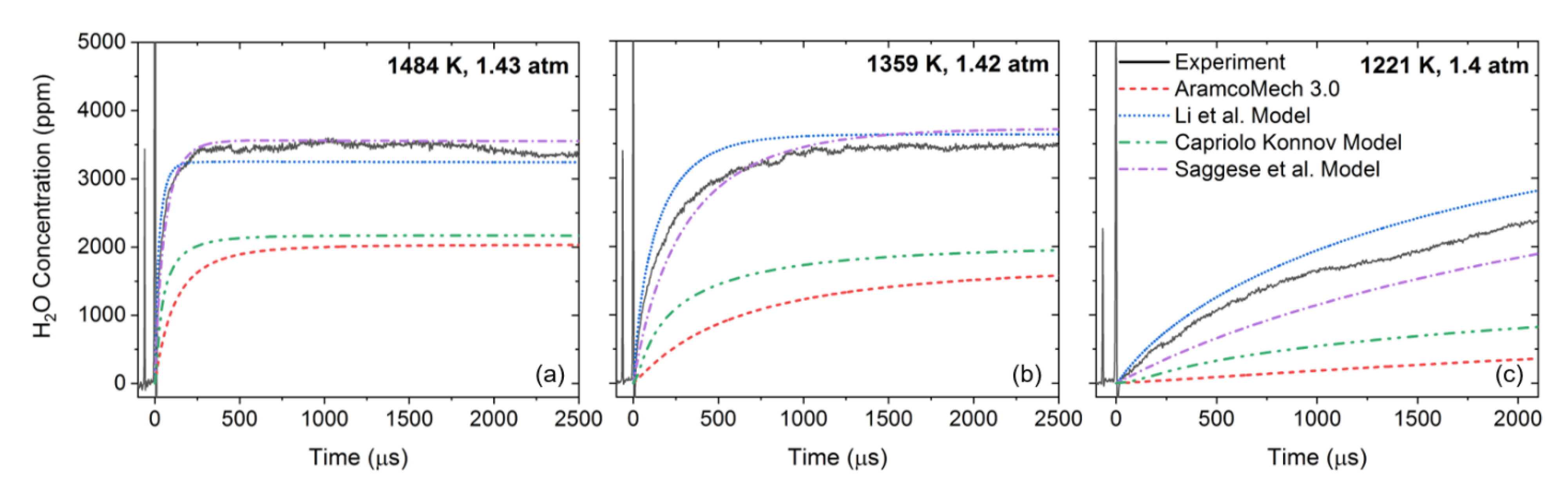
3.1. Pyrolysis
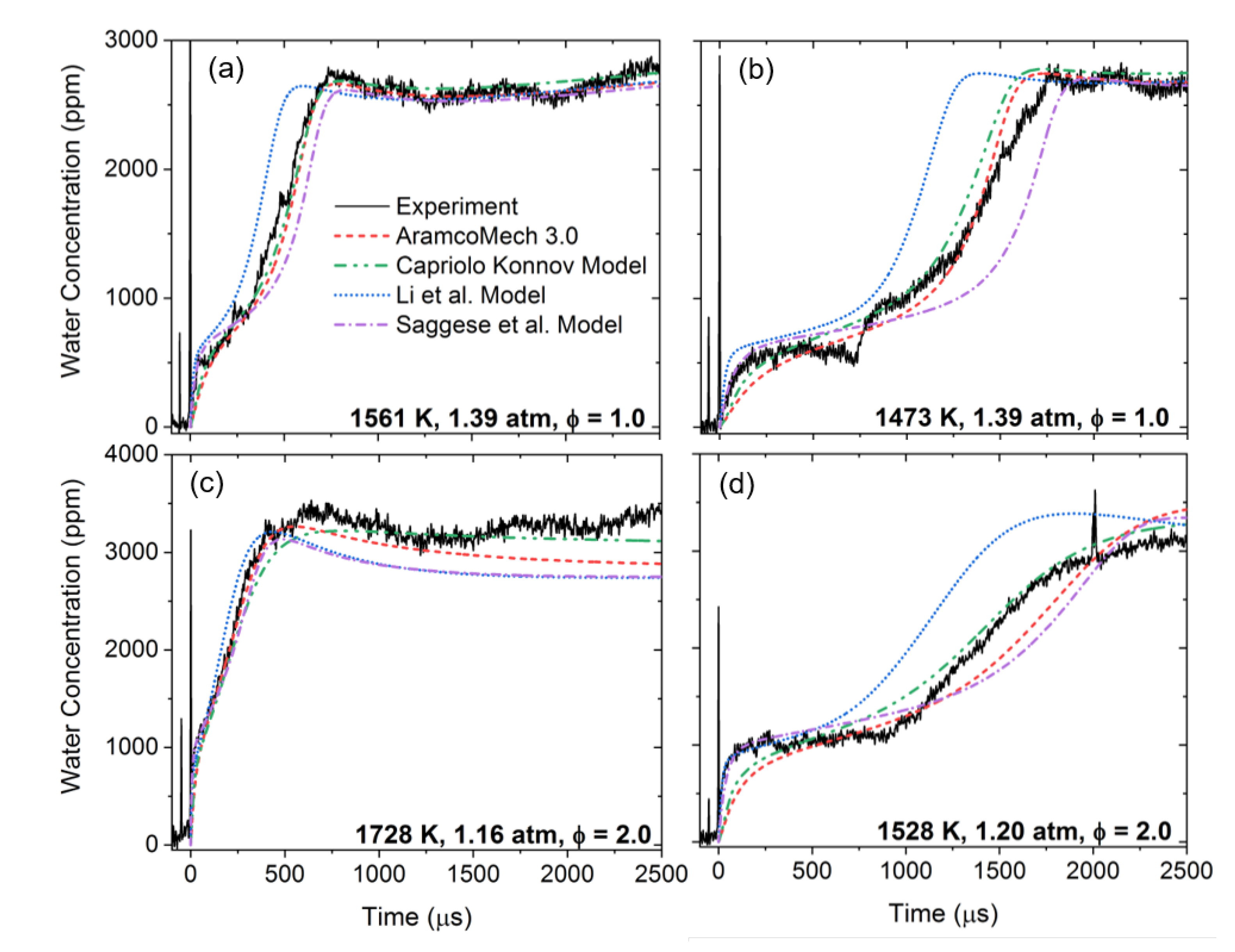
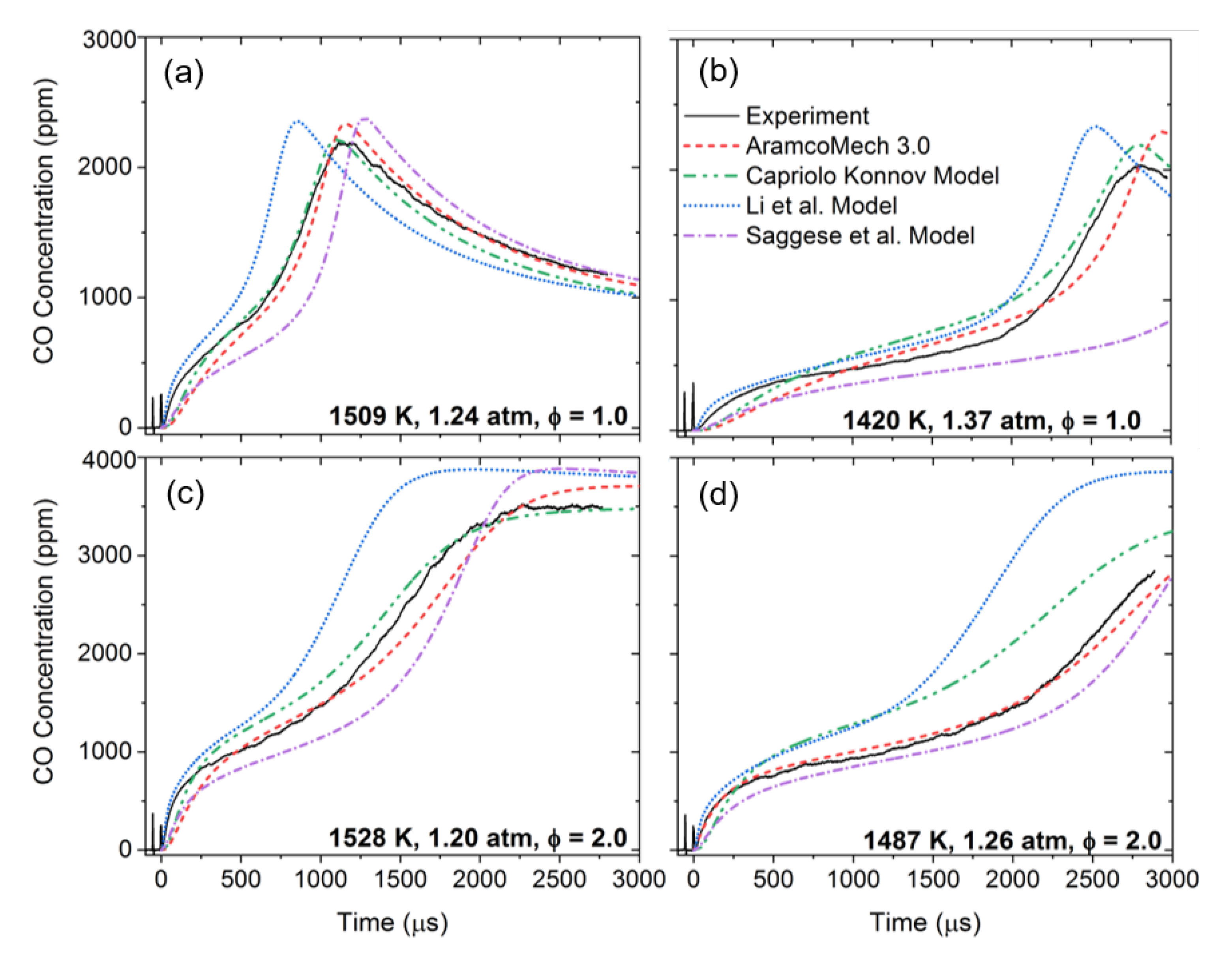
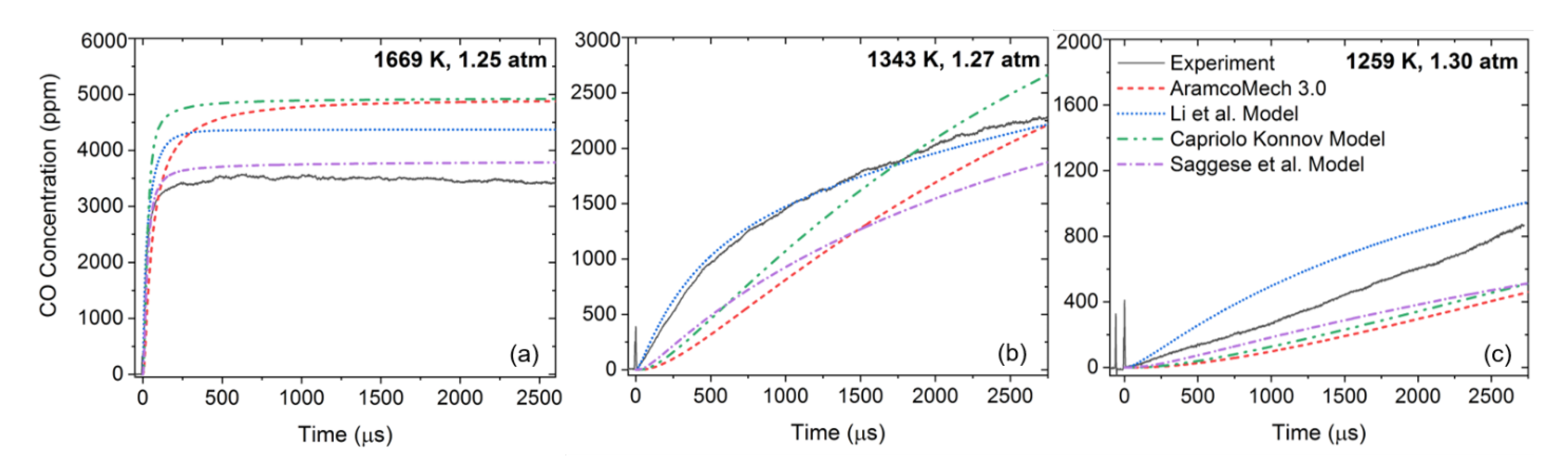
3.2. Oxidation
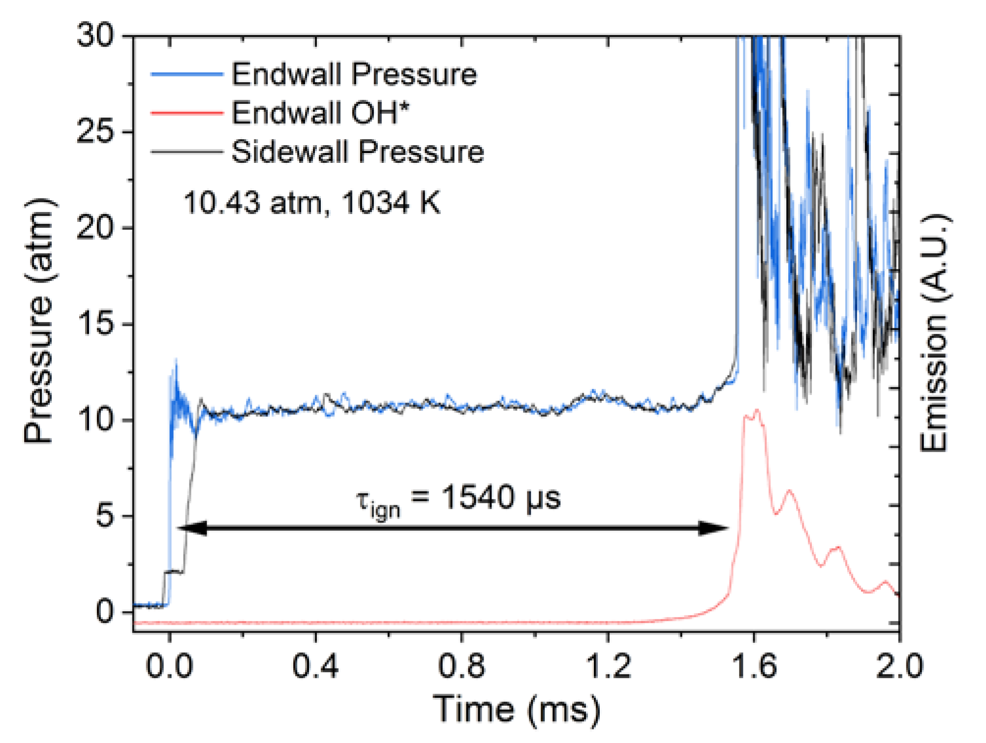
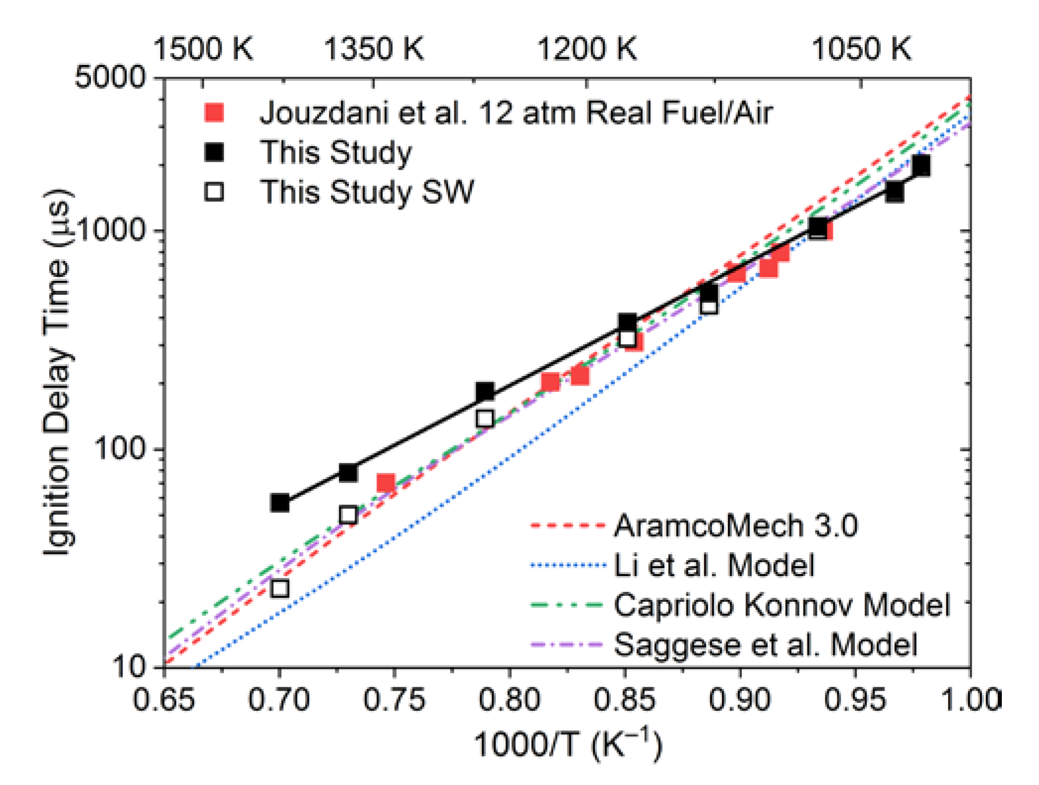
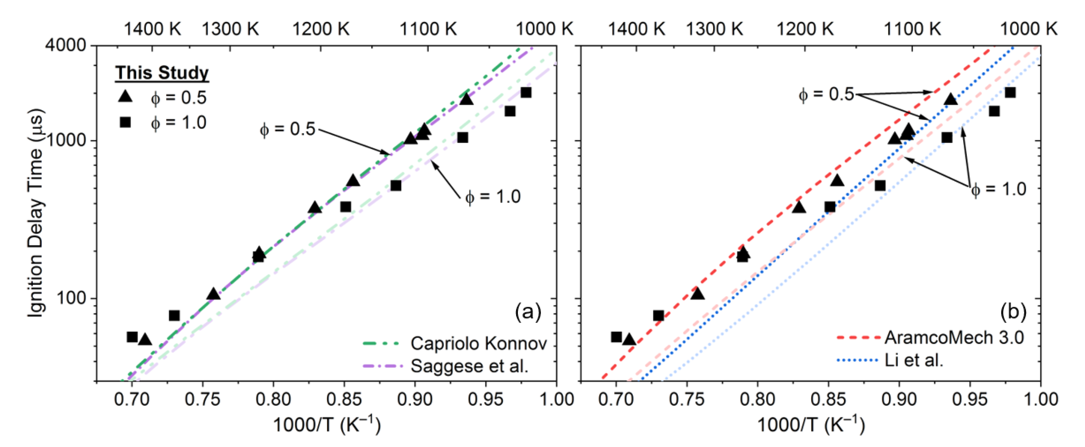
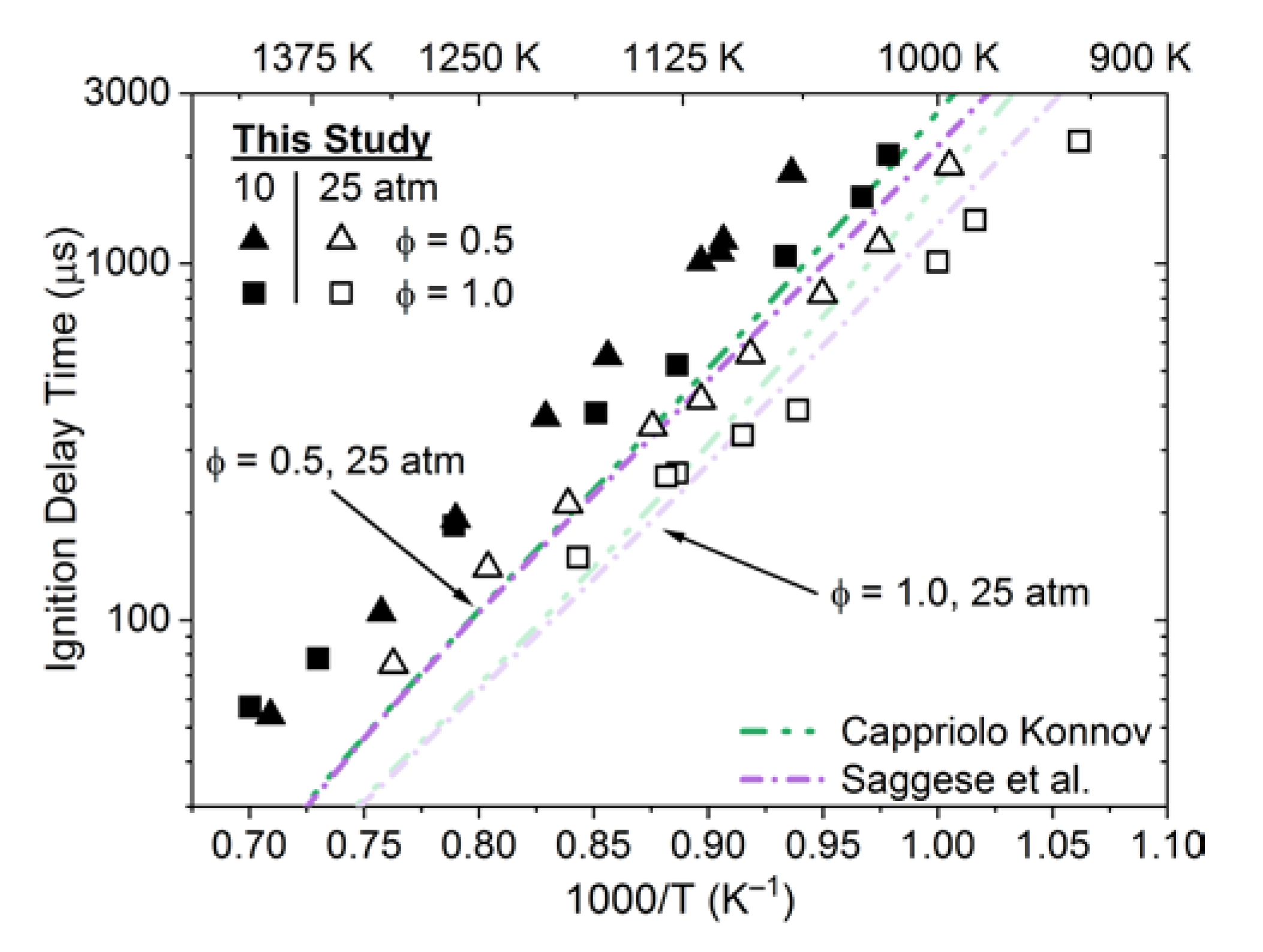
3.3. Ignition Delay Time
4. Discussion
5. Conclusions
Supplementary Materials
Author Contributions
Funding
Data Availability Statement
Acknowledgments
Conflicts of Interest
References
- Agarwal, A.K.; Kim, J. Biofuels (alcohols and biodiesel) applications as fuels for internal combustion engines. Prog. Energy Combust. Sci. 2007, 33, 233–271. [Google Scholar] [CrossRef]
- Co-Optima. Available online: https://energy.gov/eere/bioenergy/co-optimization-fuels-engines (accessed on 21 January 2019).
- McCormick, R.; Fioroni, G.; Fouts, L.; Christensen, E.; Yanowitz, J.; Polikarpov, E.; Albrecht, K.; Gaspar, D.; Gladden, J.; George, A. Selection Criteria and Screening of Potential Biomass-Derived Streams as Fuel Blendstocks for Advanced Spark-Ignition Engines. SAE Int. J. Fuels Lubr. 2017, 10, 442–460. [Google Scholar] [CrossRef]
- Gaspar, D.J.; West, B.H.; Ruddy, D.; Wilke, T.J.; Polikarpov, E.; Alleman, T.L.; George, A.; Monroe, E.; Davis, R.W.; Vardon, D.; et al. Top Ten Blendstocks Derived from Biomass for Turbocharged Spark Ignition Engines: Bio-Blendstocks with Potential for Highest Engine Efficiency; Pacific Northwest National Lab (PNNL): Richland, WA, USA, 2019. [Google Scholar]
- Mathieu, O.; Sikes, T.; Kulatilaka, W.D.; Petersen, E.L. Ignition delay time and laminar flame speed measurements of mixtures containing diisopropyl-methylphosphonate (DIMP). Combust. Flame 2020, 215, 66–77. [Google Scholar] [CrossRef]
- Fuller, M.E.; Goldsmith, C.F. Shock Tube Laser Schlieren Study of the Pyrolysis of Isopropyl Nitrate. J. Phys. Chem. A 2019, 123, 5866–5876. [Google Scholar] [CrossRef] [PubMed]
- Smith, S.R.; Gordon, A.S. Studies of Diffusion Flames. II. Diffusion Flames of Some Simple Alcohols. J. Phys. Chem. 1956, 60, 1059–1062. [Google Scholar] [CrossRef]
- Norton, T.S.; Dryer, F.L. The flow reactor oxidation of C1−C4 alcohols and MTBE. Proc. Combust. Inst. 1991, 23, 179–185. [Google Scholar] [CrossRef]
- Sinha, A.; Thomson, M. The chemical structures of opposed flow diffusion flames of C3 oxygenated hydrocarbons (isopropanol, dimethoxy methane, and dimethyl carbonate) and their mixtures. Combust. Flame 2004, 136, 548–556. [Google Scholar] [CrossRef]
- Frassoldati, A.; Cuoci, A.; Faravelli, T.; Niemann, U.; Ranzi, E.; Seiser, R.; Seshadri, K. An experimental and kinetic modeling study of n-propanol and iso-propanol combustion. Combust. Flame 2010, 157, 2–16. [Google Scholar] [CrossRef]
- Esarte, C.; Abián, M.; Millera, Á.; Bilbao, R.; Alzueta, M.U. Gas and soot products formed in the pyrolysis of acetylene mixed with methanol, ethanol, isopropanol or n-butanol. Energy 2012, 43, 37–46. [Google Scholar] [CrossRef]
- Li, W.; Zhang, Y.; Mei, B.; Li, Y.; Cao, C.; Zou, J.; Yang, J.; Cheng, Z. Experimental and kinetic modeling study of n-propanol and i-propanol combustion: Flow reactor pyrolysis and laminar flame propagation. Combust. Flame 2019, 207, 171–185. [Google Scholar] [CrossRef]
- Li, Y.; Wei, L.; Tian, Z.; Yang, B.; Wang, J.; Zhang, T.; Qi, F. A comprehensive experimental study of low-pressure premixed C3-oxygenated hydrocarbon flames with tunable synchrotron photoionization. Combust. Flame 2008, 152, 336–359. [Google Scholar] [CrossRef]
- Kasper, T.; Oßwald, P.; Struckmeier, U.; Kohse-Höinghaus, K.; Taatjes, C.; Wang, J.; Cool, T.; Law, M.; Morel, A.; Westmoreland, P. Combustion chemistry of the propanol isomers—Investigated by electron ionization and VUV-photoionization molecular-beam mass spectrometry. Combust. Flame 2009, 156, 1181–1201. [Google Scholar] [CrossRef]
- Togbé, C.; Dagaut, P.; Halter, F.; Foucher, F. 2-Propanol Oxidation in a Pressurized Jet-Stirred Reactor (JSR) and Combustion Bomb: Experimental and Detailed Kinetic Modeling Study. Energy Fuels 2011, 25, 676–683. [Google Scholar] [CrossRef]
- Johnson, M.V.; Goldsborough, S.S.; Serinyel, Z.; O’Toole, P.; Larkin, E.; O’Malley, G.; Curran, H.J. A shock tube study of n-and iso-propanol ignition. Energy Fuels 2009, 23, 5886–5898. [Google Scholar] [CrossRef]
- Akih-Kumgeh, B.; Bergthorson, J.M. Ignition of C3 oxygenated hydrocarbons and chemical kinetic modeling of propanal oxidation. Combust. Flame 2011, 158, 1877–1889. [Google Scholar] [CrossRef]
- Man, X.; Tang, C.; Zhang, J.; Zhang, Y.; Pan, L.; Huang, Z.; Law, C.K. An experimental and kinetic modeling study of n-propanol and i-propanol ignition at high temperatures. Combust. Flame 2014, 161, 644–656. [Google Scholar] [CrossRef]
- Jouzdani, S.; Zhou, A.; Akih-Kumgeh, B. Propanol isomers: Investigation of ignition and pyrolysis time scales. Combust. Flame 2017, 176, 229–244. [Google Scholar] [CrossRef]
- Cheng, S.; Kang, D.; Goldsborough, S.S.; Saggese, C.; Wagnon, S.W.; Pitz, W.J. Experimental and modeling study of C2–C4 alcohol autoignition at intermediate temperature conditions. Proc. Combust. Inst. 2021, 38, 709–717. [Google Scholar] [CrossRef]
- Cooper, S.P.; Mulvihill, C.R.; Mathieu, O.; Petersen, E.L. Isopropanol dehydration reaction rate kinetics measurement using H2O time histories. Int. J. Chem. Kinet. 2021, 53, 536–547. [Google Scholar] [CrossRef]
- Mathieu, O.; Pinzón, L.T.; Atherley, T.M.; Mulvihill, C.R.; Schoel, I.; Petersen, E.L. Experimental study of ethanol oxidation behind reflected shock waves: Ignition delay time and H2O laser-absorption measurements. Combust. Flame 2019, 208, 313–326. [Google Scholar] [CrossRef]
- Pinzón, L.T.; Mathieu, O.; Mulvihill, C.R.; Schoegl, I.; Petersen, E.L. Ethanol pyrolysis kinetics using H2O time history measurements behind reflected shock waves. Proc. Combust. Inst. 2019, 37, 239–247. [Google Scholar] [CrossRef]
- Mertens, L.A.; Manion, J.A. Kinetics of isopropanol decomposition and reaction with H atoms from shock tube experiments and rate constant optimization using the method of uncertainty minimization using polynomial chaos expansions (MUM-PCE). Int. J. Chem. Kinet. 2021, 53, 95–126. [Google Scholar] [CrossRef]
- Veloo, P.S.; Egolfopoulos, F. Studies of n-propanol, iso-propanol, and propane flames. Combust. Flame 2011, 158, 501–510. [Google Scholar] [CrossRef]
- Sarathy, S.M.; Osswald, P.; Hansen, N.; Kohse-Höinghaus, K. Alcohol combustion chemistry. Prog. Energy Combust. Sci. 2014, 44, 40–102. [Google Scholar] [CrossRef]
- Zhou, C.-W.; Li, Y.; Burke, U.; Banyon, C.; Somers, K.P.; Ding, S.; Khan, S.; Hargis, J.W.; Sikes, T.; Mathieu, O.; et al. An experimental and chemical kinetic modeling study of 1,3-butadiene combustion: Ignition delay time and laminar flame speed measurements. Combust. Flame 2018, 197, 423–438. [Google Scholar] [CrossRef]
- Liu, X.; Wang, H.; Zheng, Z.; Liu, J.; Reitz, R.D.; Yao, M. Development of a combined reduced primary reference fuel-alcohols (methanol/ethanol/propanols/butanols/n-pentanol) mechanism for engine applications. Energy 2016, 114, 542–558. [Google Scholar] [CrossRef]
- Capriolo, G.; Konnov, A. Combustion of propanol isomers: Experimental and kinetic modeling study. Combust. Flame 2020, 218, 189–204. [Google Scholar] [CrossRef]
- Saggese, C.; Thomas, C.M.; Wagnon, S.W.; Kukkadapu, G.; Cheng, S.; Kang, D.; Goldsborough, S.S.; Pitz, W.J. An improved detailed chemical kinetic model for C3-C4 linear and iso-alcohols and their blends with gasoline at engine-relevant conditions. Proc. Combust. Inst. 2021, 38, 415–423. [Google Scholar] [CrossRef]
- Petersen, E.; Rickard, M.J.A.; Crofton, M.W.; Abbey, E.D.; Traum, M.J.; Kalitan, D.M. A facility for gas- and condensed-phase measurements behind shock waves. Meas. Sci. Technol. 2005, 16, 1716–1729. [Google Scholar] [CrossRef]
- Lipkowicz, J.T.; Nativel, D.; Cooper, S.; Wlokas, I.; Fikri, M.; Petersen, E.; Schulz, C.; Kempf, A.M. Numerical Investigation of Remote Ignition in Shock Tubes. Flow, Turbul. Combust. 2021, 106, 471–498. [Google Scholar] [CrossRef]
- Mulvihill, C.R.; Alturaifi, S.A.; Petersen, E.L. A shock-tube study of the N2O + M ⇄ N2 + O + M (M = Ar) rate constant using N2O laser absorption near 4.6 µm. Combust. Flame 2021, 224, 6–13. [Google Scholar] [CrossRef]
- Vivanco, J.E. A New Shock-Tube Facility for the Study of High-Temperature Chemical Kinetics. Master’s Thesis, Texas A&M University, College Station, TX, USA, 2014. [Google Scholar]
- Zander, L.; Vinkeloe, J.; Djordjevic, N. Ignition delay and chemical–kinetic modeling of undiluted mixtures in a high-pressure shock tube: Nonideal effects and comparative uncertainty analysis. Int. J. Chem. Kinet. 2021, 53, 611–637. [Google Scholar] [CrossRef]
- Hargis, J.W.; Petersen, E.L. Shock-Tube Boundary-Layer Effects on Reflected-Shock Conditions with and without CO2. AIAA J. 2017, 55, 902–912. [Google Scholar] [CrossRef]
- Nativel, D.; Cooper, S.P.; Lipkowicz, T.; Fikri, M.; Petersen, E.L.; Schulz, C. Impact of shock-tube facility-dependent effects on incident- and reflected-shock conditions over a wide range of pressures and Mach numbers. Combust. Flame 2020, 217, 200–211. [Google Scholar] [CrossRef]
- Alturaifi, S.A.; Rebagay, R.L.; Mathieu, O.; Guo, B.; Petersen, E.L. A Shock-Tube Autoignition Study of Jet, Rocket, and Diesel Fuels. Energy Fuels 2019, 33, 2516–2525. [Google Scholar] [CrossRef]
- Cooper, S.P.; Mathieu, O.; Schoegl, I.; Petersen, E.L. High-pressure ignition delay time measurements of a four-component gasoline surrogate and its high-level blends with ethanol and methyl acetate. Fuel 2020, 275, 118016. [Google Scholar] [CrossRef]
- Mathieu, O.; Mulvihill, C.; Petersen, E.L. Shock-tube water time-histories and ignition delay time measurements for H2S near atmospheric pressure. Proc. Combust. Inst. 2017, 36, 4019–4027. [Google Scholar] [CrossRef] [Green Version]
- Mulvihill, C.R.; Petersen, E.L. Concerning shock-tube ignition delay times: An experimental investigation of impurities in the H2/O2 system and beyond. Proc. Combust. Inst. 2019, 37, 259–266. [Google Scholar] [CrossRef]
- Mathieu, O.; Mulvihill, C.; Petersen, E.L. Assessment of modern detailed kinetics mechanisms to predict CO formation from methane combustion using shock-tube laser-absorption measurements. Fuel 2019, 236, 1164–1180. [Google Scholar] [CrossRef]
- Mathieu, O.; Cooper, S.; Alturaifi, S.A.; Mulvihill, C.R.; Atherley, T.; Petersen, E.L. Shock-Tube Laser Absorption Measurements of CO and H2O during Iso-Octane Combustion. Energy Fuels 2020, 34, 7533–7544. [Google Scholar] [CrossRef]
- Mulvihill, C.R.; Keesee, C.L.; Sikes, T.; Teixeira, R.S.; Mathieu, O.; Petersen, E.L. Ignition delay times, laminar flame speeds, and species time-histories in the H2S/CH4 system at atmospheric pressure. Proc. Combust. Inst. 2019, 37, 735–742. [Google Scholar] [CrossRef]
- Petersen, E.L. Interpreting Endwall and Sidewall Measurements in Shock-Tube Ignition Studies. Combust. Sci. Technol. 2009, 181, 1123–1144. [Google Scholar] [CrossRef]
- Ansys. ChemKin 19.1; Ansys: San Diego, CA, USA, 2018. [Google Scholar]
- Pelucchi, M.; Cavallotti, C.; Faravelli, T.; Klippenstein, S.J. H-Abstraction reactions by OH, HO2, O, O2 and benzyl radical addition to O2 and their implications for kinetic modelling of toluene oxidation. Phys. Chem. Chem. Phys. 2018, 20, 10607–10627. [Google Scholar] [CrossRef] [PubMed]
- Cai, J.; Zhang, L.; Zhang, F.; Wang, Z.; Cheng, Z.; Yuan, W.; Qi, F. Experimental and Kinetic Modeling Study of n-Butanol Pyrolysis and Combustion. Energy Fuels 2012, 26, 5550–5568. [Google Scholar] [CrossRef]
- Jin, H.; Cai, J.; Wang, G.; Wang, Y.; Li, Y.; Yang, J.; Cheng, Z.; Yuan, W.; Qi, F. A comprehensive experimental and kinetic modeling study of tert-butanol combustion. Combust. Flame 2016, 169, 154–170. [Google Scholar] [CrossRef]
- Sarathy, S.M.; Vranckx, S.; Yasunaga, K.; Mehl, M.; Osswald, P.; Metcalfe, W.K.; Westbrook, C.K.; Pitz, W.J.; Kohse-Höinghaus, K.; Fernandes, R.X.; et al. A comprehensive chemical kinetic combustion model for the four butanol isomers. Combust. Flame 2012, 159, 2028–2055. [Google Scholar] [CrossRef]
- Tsang, W.; Walker, J.A.; Manion, J.A. The decomposition of normal hexyl radicals. Proc. Combust. Inst. 2007, 31, 141–148. [Google Scholar] [CrossRef]
- Heyne, J.S.; Dooley, S.; Serinyel, Z.; Dryer, F.L.; Curran, H. Decomposition Studies of Isopropanol in a Variable Pressure Flow Reactor. Zeitschrift für Physikalische Chemie 2015, 229, 881–907. [Google Scholar] [CrossRef] [Green Version]
- Sen, F.; Shu, B.; Kasper, T.; Herzler, J.; Welz, O.; Fikri, M.; Atakan, B.; Schulz, C. Shock-tube and plug-flow reactor study of the oxidation of fuel-rich CH4/O2 mixtures enhanced with additives. Combust. Flame 2016, 169, 307–320. [Google Scholar] [CrossRef]


| Mixture Composition (% mol) | Conditions | ||||||
|---|---|---|---|---|---|---|---|
| Mix | iC3H7OH | O2 | Diluent | ϕ | P5 (atm) | T5 (K) | Measurement |
| 1 | 0.75% | N/A | 99.25% Ar | Inf. | 1.42 ± 0.10 | 1127–2162 | Water Abs. |
| 2 | 0.75% | N/A | 20.07% He + 79.18% Ar | Inf | 1.29 ± 0.09 | 1173–1669 | Water and CO Abs. |
| 3 | 0.05% | 0.45% | 20.11% He + 79.39% Ar | 0.5 | 1.28 ± 0.07 | 1341–1519 | |
| 4 | 0.09% | 0.41% | 20.08% He + 79.42% Ar | 1.0 | 1.25 ± 0.12 | 1416–1646 | |
| 5 | 0.09088% | 0.4112% | 99.7492% Ar | 1.0 | 1.36 ± 0.15 | 1419–2073 | |
| 6 | 0.1540% | 0.3444% | 20.0456% He + 79.456% Ar | 2.0 | 1.22 ± 0.06 | 1470–1728 | |
| 7 | 2.281% | 20.529% | 77.19% N2 | 0.5 | 10.2 ± 0.8 | 1068–1410 | OH* τign |
| 24.5 ± 3.4 | 995–1311 | ||||||
| 8 | 4.46% | 20.07% | 75.47% N2 | 1.0 | 10.2 ± 1.2 | 1022–1428 | |
| 26.5 ± 3.2 | 942–1186 | ||||||
| Model | # Species | # Reactions | Year |
|---|---|---|---|
| AramcoMech 3.0 | 581 | 3037 | 2018 |
| Li et al. | 156 | 1394 | 2019 |
| Capriolo and Konnov | 161 | 1787 | 2020 |
| Saggese et al. | 371 | 2318 | 2020 |
| Model | A (s−1) | n | Ea (cal/mol) |
|---|---|---|---|
| Li et al. | 1.87 × 1038 | −6.8 | 81,200 |
| AramcoMech 3.0 | 5.00 × 10¹³ | 0 | 68,000 |
| Capriolo and Konnov | 5.00 × 10¹³ | 0 | 68,000 |
| Saggese et al. | 8.52 × 10⁶ | 2.12 | 60,935 |
Publisher’s Note: MDPI stays neutral with regard to jurisdictional claims in published maps and institutional affiliations. |
© 2021 by the authors. Licensee MDPI, Basel, Switzerland. This article is an open access article distributed under the terms and conditions of the Creative Commons Attribution (CC BY) license (https://creativecommons.org/licenses/by/4.0/).
Share and Cite
Cooper, S.P.; Grégoire, C.M.; Mohr, D.J.; Mathieu, O.; Alturaifi, S.A.; Petersen, E.L. An Experimental Kinetics Study of Isopropanol Pyrolysis and Oxidation behind Reflected Shock Waves. Energies 2021, 14, 6808. https://doi.org/10.3390/en14206808
Cooper SP, Grégoire CM, Mohr DJ, Mathieu O, Alturaifi SA, Petersen EL. An Experimental Kinetics Study of Isopropanol Pyrolysis and Oxidation behind Reflected Shock Waves. Energies. 2021; 14(20):6808. https://doi.org/10.3390/en14206808
Chicago/Turabian StyleCooper, Sean P., Claire M. Grégoire, Darryl J. Mohr, Olivier Mathieu, Sulaiman A. Alturaifi, and Eric L. Petersen. 2021. "An Experimental Kinetics Study of Isopropanol Pyrolysis and Oxidation behind Reflected Shock Waves" Energies 14, no. 20: 6808. https://doi.org/10.3390/en14206808
APA StyleCooper, S. P., Grégoire, C. M., Mohr, D. J., Mathieu, O., Alturaifi, S. A., & Petersen, E. L. (2021). An Experimental Kinetics Study of Isopropanol Pyrolysis and Oxidation behind Reflected Shock Waves. Energies, 14(20), 6808. https://doi.org/10.3390/en14206808