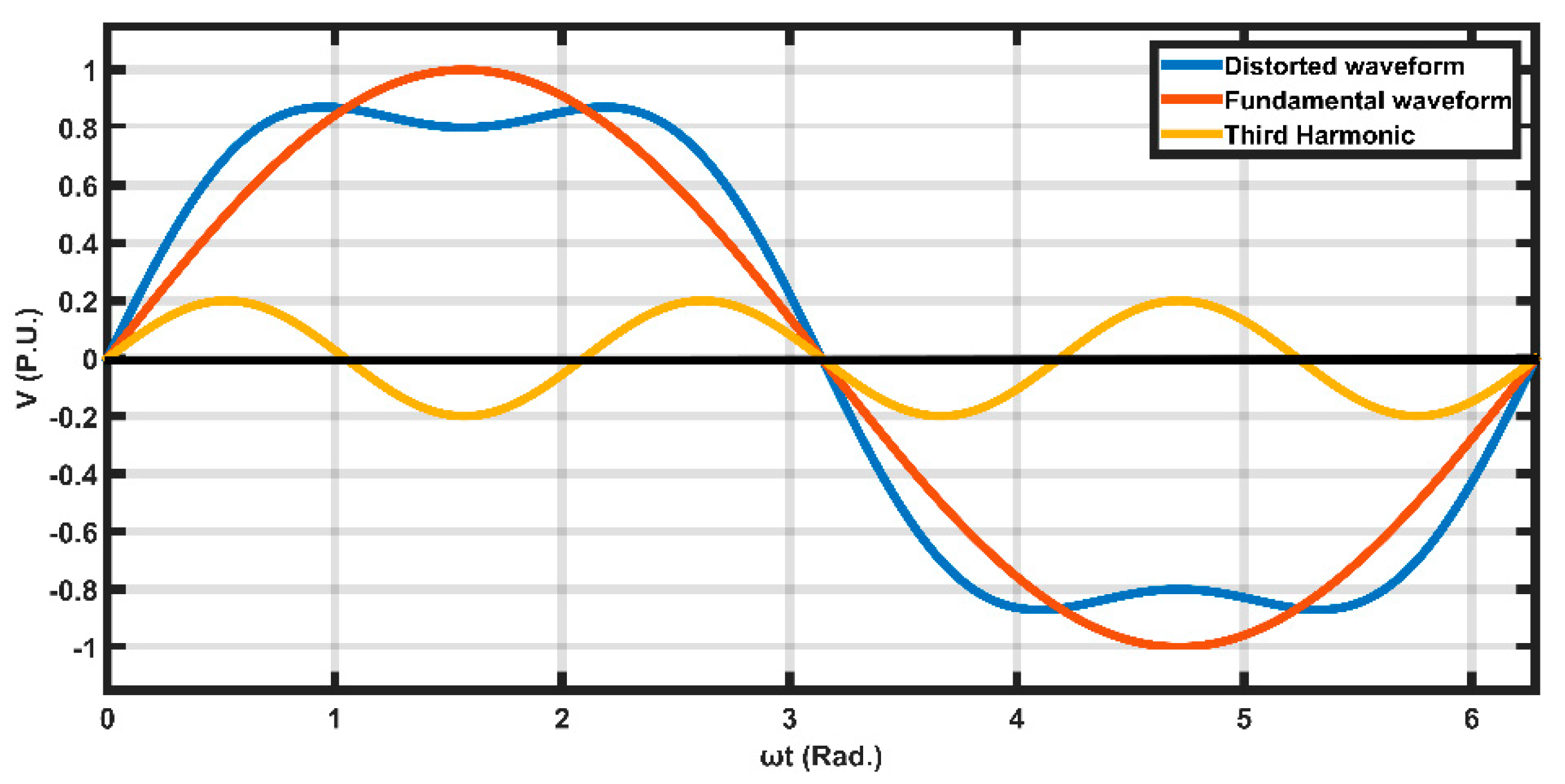
Article

Reduction of Total Harmonic Distortion of Wind Turbine Active Power Using Blade Angle Adaptive PI Controller

by
Ahmed M. Shawqran
1,
Abdallah El-Marhomy
1,
Mariam A. Sameh
2,* and
Mahmoud A. Attia
3
1
Physics and Engineering Mathematics Department, Faculty of Engineering, Ain Shams University, Cairo 11835, Egypt
2
Electrical Engineering Department, Faculty of Engineering, Future University in Egypt, Cairo 11835, Egypt
3
Electrical Power and Machines Department, Faculty of Engineering, Ain Shams University, Cairo 11835, Egypt
*
Author to whom correspondence should be addressed.
Energies 2021, 14(20), 6798; https://doi.org/10.3390/en14206798
Submission received: 23 July 2021 / Revised: 16 September 2021 / Accepted: 18 September 2021 / Published: 18 October 2021

Abstract

:
Power quality can have a large detrimental effect on industrial processes and the commercial sector. Thus, this paper proposes a new technique to improve the power quality of electric power systems. This technique relies on auto-adjusting of the blade angle to mitigate the harmonics in wind generator active power. A new adaptive PI blade-angle controller is applied in this technique to reduce the total harmonic distortion (THD) of the output power. The parameters of the adaptive PI controller are initialized by using the Harmony Search algorithm (HSA), hybrid Harmony Search optimization and Equilibrium optimization (EO), and hybrid Harmony Search optimization and Teaching learning-based optimization (TLBO). The execution of the optimization algorithms relies mainly on the optimization objective function. Two optimization objective functions are mathematically modeled and compared to enhance the power quality. The first one is to minimize the sum square of error, while the second objective is to minimize the THD. Many case studies are applied with various wind-speed profiles under normal and faulty conditions. Results show the superiority of HSA hybrid EO algorithm with the second objective functions through reducing the harmonics and enhancing the power quality. Moreover, laboratory studies are applied to investigate the effect of the blade-angle variations on the extracted active power.

1. Introduction

Due to the rising demand for wind energy, power quality has become a significant issue. Wind power plants should ensure the stability and reliability of the power system by achieving the required power-quality standards. The main problems of the wind-system power quality are voltage deviation, voltage flicker, voltage fluctuation, and harmonic distribution [1,2].
In the presented research work, only the power quality harmonics issue is considered. Harmonics in electric power systems can cause several complications; as in doubly fed induction generators (DFIG), the unwanted harmonic current can cause torque pulsations, more copper-winding losses, and thermal effects on transformers and rotating machines. Harmonics may also excite mechanical resonance modes of the wind-turbine components [3].
The harmonics are mainly composed due to nonlinear loads. Moreover, in DFIG wind turbines, power converters that control the real and reactive power can generate harmonics due to their nonlinear devices. Furthermore, harmonics can be generated by the rotor non-sinusoidal conditions and the unbalance stator voltages. Unbalanced stator voltages can be resolved into three sequences: positive, negative, and zero-sequence voltages. These negative sequence components can cause the generation of high-frequency components in rotor currents and torque pulsations which may cause overheat [4,5].
Many approaches have been applied to decrease the total harmonic distortion such as: passive filters, active filters (shunt active power filter and series active power filter), band pass filters (single tuned and double tuned), hybrid filters, and flexible AC transmission systems (FACTS) devices, such as the Static Synchronous Compensator (STATCOM) and Static Synchronous Series Compensator (SSSC) [6,7].
Conventionally, many researches implement passive filters to reduce the current harmonics due to nonlinear loads. However, the passive filters fail to solve random variations in the load current waveforms [8]. Active power filters have been developed to overcome the disadvantages of passive filters and to provide a more flexible and reliable compensation [9].
Active harmonic filters are controlled current sources that can eliminate the existing harmonics by injecting the same harmonic with phase angle opposite to the existing ones to cancel them out. They are connected in parallel to the load. They are also used for reactive power compensation (PF Correction), harmonic filtering, and flicker reduction (active power provision).
In References [10,11], the authors claimed that the STATCOM can compensate for both current harmonics and power factor in a three-phase power system with neutral line. Furthermore, it allows load balancing, eliminating the current in the neutral line.
The Static Synchronous Series Compensator (SSSC) acts as a variable reactance compensator; it can vary the injected voltage magnitude V q in quadrature with current, so the SSSC can be either capacitive or inductive. It also reduces the THD. The gains of the SSSC are tuned by using different optimization algorithms, such as the Harmony Search algorithm (HSA). A comparison proves the superiority of a SSSC device to FACT devices [12].
Several controllers are used in blade-angle controller systems, such as fuzzy logic, slide mode controller, PID controller, H controller, and neural network control. In Refs. [13,14], a PID controller was used in all wind-turbine power regions, but the controller reliability was affected by the nonlinear behavior of the wind-turbine parameters. Fuzzy logic control is more suitable to the nonlinear systems [13]. Fuzzy controller is used to extract more power at low wind-speed conditions, while protecting the system at high wind-speed condition [15]. Ref. [16] found that the sliding mode control is the most suitable controller to deal with time varying parameters in the nonlinear systems. The authors of Ref. [17] proved that the neural network controller is suitable for dealing with high wind-speed conditions where the neural network does not depend on the system mathematical model. The main advantage of the H controller is not depending on the system parameters [18].
The main disadvantages of the previous controllers are that some of them depend on the wind mathematical model, such as H , and sliding mode controllers. Others have difficulties in adjusting and training the weighting coefficients, as in fuzzy logic and neural network controllers. Moreover, the PID controller is not suitable for nonlinear systems, and its gains are not auto-adjusted [18].
In this article, a new approach is applied to suppress the total harmonic distortion of active power. This approach readjusts the blade angles of the horizontal axis wind turbine model DFIG, using an adaptive PI (API) controller. The gains of the controller are initialized by using different heuristics optimization algorithms. Section 2 defines the total harmonic distortion. Section 3 discusses the effects of variation of blade angle through laboratory case studies, using the Lucus-NÜLLE GmbH Model wind power plant. Section 4 provides the wind turbine system model and adaptive PI controller model. In Section 5, three optimization algorithms are proposed. Section 6 gives the results of different simulation studies under normal and faulty conditions. Finally, the conclusion is determined.

2. Total Harmonic Distortion (THD)

The harmonics frequency can be defined as follows:
f n = n   f
where n is a positive integer that represents the harmonic order. When n < 1, it is called sub-harmonics [19]. Figure 1 shows a waveform that contains first and third harmonics. In the description of the harmonic order, there are three types of harmonics: even harmonics, odd harmonics, and define triplet harmonics. The harmonic sequence has three harmonic sequences: positive sequence, negative sequence, and zero sequence harmonics [20].
There are two main definitions for total harmonic distortion. Originally, it was defined as the harmonic components of a waveform compared to the fundamental component [21,22]. Moreover, it can be defined as the harmonic components compared to the waveform’s root mean square (RMS) components [23]. At low values of THD, the two definitions nearly give the same values. Thus, THD is defined as follows [24]:
T H D = n = 2 I n 2 I 1
where I n is the current of the nth harmonic; n is the harmonic value, and all possible harmonics are included; and I1 is the nominal system current at the fundamental frequency. The first definition is used in this paper. Moreover, T H D 1 and T H D 2 are the total harmonic distortion of voltage, V, and power, P, respectively, as shown in following equations:
T H D 1 = n = 2 V h 2 V 1 = V 2 2 + + V h 2   V 1
T H D 2 = n = 2 P h 2 P 1 = P 2 2 + + P h 2   P 1
The standard limits of the total harmonic distortion (THD) in any power system are listed in (ANSI/IEEE 519-1992) standard lists [25,26]. Thus, the analysis of the harmonics of the system and the system installation should meet standard (IEEE 519-1992) to limit the THD [27].
The distortion power or the distortion volt-amperes is given by the quantity D. It represents all cross products of voltage and current at different frequencies. The quantity D cannot be defined as power, because it does not flow through the system. The quantity Q represents the sum of the traditional reactive power values at each frequency. P, Q, D, and S are correlated as follows:
S = P 2 + Q 2 + D 2
P F = P S  
This power factor is called the distorted power factor, and it is caused by the harmonics [28].

3. Laboratory Studies

The operation of the blade-angle controller is divided into four main regions, as shown in Figure 2. Before the cut in speed (nearly 4.9 m/s), no electric power is generated. Between the cut in speed and the rated speed (nearly 12 m/s), the controller aims to maximize the generated power (maximum power point tracking MPPT). Above the rated speed, the controller function is to regulate the generated power at rated value. Regions two and three are known as the utilized power range. At high gust-wind speeds (above 25 m/s), the turbine should be locked to protect the turbine (shutdown power range) [29].
The impact of changing the blade angle on the turbine output power can be illustrated inside the Laboratory. The LUCAS-NÜLLE GmbH model wind power plant connection diagram is shown in Figure 3a. All the scenarios of practical relevance are emulated under different wind-speed profiles, with the aid of the wind turbine controller. The LUCAS-NÜLLE GmbH Model wind lab is composed of the following [30,31]:
  • Wind-turbine control unit that comprises two three-phase inverters;
  • A 400/230 V rated voltage three-phase DFIG generator of 0.8 kW rated power;
  • A 1 KVA rated power three-phase transformer;
  • A variable output voltage (0–240 V) power supply with (3–10 A) adjustable limit output current;
  • Three-phase meters.
Figure 3b shows the wind power plant laboratory setup. Initially, the DFIG is set at the synchronization speed (4.9 m/s) with zero pitch angle. At this speed, the generator stator side is connected to the grid.
The wind turbine control unit allows three modes of operation: fixed speed fixed pitch (FSFP), variable speed fixed pitch (VSFP), and variable speed variable pitch (VSVP).
The first mode of operation is applied at different wind speeds: 5, 6, and 7 m/s. The blade angle is varied from zero degree to 15 degrees with step size 5 degrees. The active power is directly proportional to the cubic of the velocity. The maximum active power is achieved at zero blade angle and is inversely proportional with the blade angle, as shown in Figure 4a–c.
In Ref. [31], the second mode is applied, and the results show that the maximum power is achieved at zero blade angle, and that there is an inverse relation between the blade angle and the output active power. In this paper, the third mode is applied to discuss the blade-angle variations through the four regions of blade-angle control.
The third mode of operation (VSVP) is applied through four different case studies at four different wind-speed profiles, as shown in Figure 5, Figure 6, Figure 7 and Figure 8. Below the cut in speed (4.9 m/s) the WT is not able to generate power at all. Between 4.9 and 9 m/s (rated speed), the blade angle is automatically tuned to reach the maximum allowable power by keeping the blade angle at zero degree (MPPT). Above the 9 m/s, the rated power (150 watt) is reached, and the blade angle’s function is to regulate this rated power. Power regulation occurs by increasing the blade angle to keep up with the increase of wind speed.

4. System Modeling

4.1. Wind Turbine Model

The wind-power system is simulated on SIMULINK/MATLAB, as shown in Figure 9. It is connected to an infinity source (120 KV) through 25 km transmission line. The wind power plant consists of six wind turbines, each of 1.5 MW rated power. Each wind turbine consists of a doubly fed induction generator (DFIG) and a protection system, which is used to continuously monitor the voltage, current, and the machine speed. The API controller is inside the wind-turbine doubly fed block.

4.2. Adaptive PI Blade-Angle-Controller Model

The adaptive PI is expressed as follows [32,33,34]:
Output ( t ) = K c ( K p ( t ) e ( t ) + 0 t K i ( t ) e ( t ) d t )
where e(t) is the error signal, K c is a constant value, K p is the proportional gain, and K i is the integral gain. The integral and proportional gains are expressed as follows [32,33,34]:
K p ( t ) = e 2 ( t ) + K 1 0 t e 2 ( t ) d t
K i ( t ) = K 2 0 t e 2 ( t ) d t
The parameters of the controller are K 1 , K 2 , and K c [32,33]. The previous equations show that the controller gains ( K p , K i ) are time-varying quantities, and this is an advantage over the conventional PID controller. The K p and K i are adjusted by the square of error signal and controller parameters to withstand any variation in the wind-speed profile or the system parameters. The adaptive PI controller block diagram is shown in Figure 10.

4.3. Blade-Angle Mechanical Delay

There are limitations to the rate of change of the blade angle ( β ), due to the mechanical delay of the servo motors that are responsible for blades rotation. These limitations are expressed as follows:
2   deg / s   d β d t   2   deg / s
Moreover, the operating range of the blade angle is limited between zero to 45°.

5. Optimization Algorithms

5.1. Optimization Algorithm

Recently, different classical and heuristics optimization algorithms are applied to enhance the performance of the system and increase its reliability. Three heuristic optimization algorithms are proposed to initialize the adaptive PI controller parameters.

5.1.1. Harmony Search Algorithm (HSA)

The Harmony Search algorithm is a meta-heuristic algorithm which relies on the improvisation process of musicians [35].
The implementation of the HS algorithm follows these steps:
Step1: Initialization of harmony memory (HM).
Step2: Improvisation of new harmony.
Step3: The new harmony is included in the HM or excluded.
Step4: repeating Steps 2 and 3 until stopping criteria are met.
Step5: optimum solution is obtained.

5.1.2. Teaching Learning-Based Optimization (TLBO)

Similar to other nature-based algorithms, TLBO is considered as a population method that uses population of solutions. It relies mainly on group of learners and two phases: learning phase and teaching phase [36].

5.1.3. Equilibrium Optimization (EO)

The EO algorithm relies on the volume balance models. These models are used to estimate both equilibrium and dynamic states. The algorithm consists mainly of particles; each particle has its own concentration. This group of particles acts as search agents [37].

5.1.4. Hybrid Optimization Algorithm (HSATLBO, HSAEO)

Hybrid optimization combines two optimization algorithms and applies it to reach the optimal solution. In this algorithm, initially, HSA is applied, and its optimum solution is obtained. The obtained optimum solution is tolerated by ±10% and used as an input range for both TLBO and EO optimization algorithms.

5.2. Objective Function

Two different objective functions are identified for the proposed problem. One is the voltage and power error objective function, and the second one is the total harmonic distortion objective function.

5.2.1. Error Objective Function

The error objective function is defined by the summation of the square of error in both signals: voltage signal and power signal. The two signals (voltage and power) are compared with reference signal and the square of error of both signals are finally summed. The main purpose of the optimization algorithm is to minimize this sum square of errors. The error in the voltage signal ( E v ) is given in Equation (11):
E v = voltage   reference measured   voltage   signal
The error in the power signal ( E p ) is given in Equation (12):
E p = power   reference measured   power   signal
The equation of objective is given in Equation (13):
Objective   one = E v 2 d t + E p 2 d t

5.2.2. Total Harmonic Distortion (THD) Objective Function

The total harmonic distortion is determined from the power signal. The mathematical model of the THD calculates the first five harmonics, using only Fast Fourier transform analysis (FFT) [38]. Reducing the THD is the objective of the algorithms. The objective two equation is given as Equation (14):
O b j e c t i v e   T w o = n = 2 P h 2 P 1

6. Normal and Faulty Case Studies

The simulated case studies include a comparison between the proposed adaptive PI controller with the conventional PID controller to prove that the adaptive PI is as good as or better than the PID controller. Moreover, the case studies include a comparison between the two objective functions: error objective (Section 5.2.1) and THD objective (Section 5.2.2). The comparison is carried out at normal and LG (line-ground) faulty conditions.
In Ref. [33], we proved the superiority of the adaptive PI over the PID controller. Moreover, it was shown that the hybrid (HSA-TLBO) shows better response than HSA and other optimization algorithms.

6.1. Normal Cases

The blade angles of the turbine are tuned by the PID controller with the error objective function, while they are tuned by the adaptive PI controller with both the error objective and THD objective functions. The algorithms are applied to initialize the controller’s parameters, which are listed in Table 1. These parameters are used in all normal cases.

6.1.1. Normal First Case

The first case is the validation case study of the proposed controller with the new objective function (THD objective). Figure 11 shows the wind-speed profile applied to wind turbine.
The active power responses for the adaptive PI controller show better performance with lower oscillations than the conventional PID, as shown in Figure 12a. The active powers of the three API controllers are superimposed under the green curve. The power responses for the adaptive PI (HSA-EO) controller with the two objective functions are nearly the same. The API HAS-EO with objective two has the lowest steady state error, as shown in Figure 12b.
The blade angles of the controllers are shown in Figure 12b. The blade angle of the PID starts from zero value to acquire less rising time, but it failed to keep up with the wind-speed fluctuations. Meanwhile, the adaptive PI blade angles overcame the wind-speed fluctuations and regulated the power.
The numerical comparisons of the controllers are listed in Table 2. The adaptive PI controllers outperform the classical PID. The differences between the three adaptive PI controllers are very small. The active power statistical analysis of each controller is given in Table 3.
The K p and K i parameters of the adaptive PI are shown in Figure 13a,b, respectively. The results show the advantage of the adaptive PI with time-varying parameters that continuously vary with wind-speed fluctuations to the PID with constant parameters.
The total harmonic distortion of the active power with different control strategies are shown in Figure 14. The adaptive PI shows lower THD compared to the PID controller. Moreover, for the adaptive PI, the THD objective function (Obj. 2) shows lower THD than the error objective function (Obj. 1). The power THD of API with objective two is 7.1189% at bus voltage equal to 575 volts, as shown in Figure 14. The IEEE standard 519-2014 did not define the power THD limits, while it defined the accepted limit of voltage THD at bus voltage (≤1 kv) to be less than or equal to 8% [41].

6.1.2. Normal Second Case

Another wind-speed profile is applied to the wind turbine, as shown in Figure 15. Figure 16a,b shows the active power and blade-angle responses of the adaptive PI with different objective functions. The performance of the new objective function is better with no oscillations and less settling time. Figure 17a,b shows the adaptive PI K p and K i gains, respectively.
The numerical comparisons of the controllers are listed in Table 4. The three adaptive PI controllers have nearly the same rising time. The API HSA-TLBO and API HSA-EO with objective two have no oscillations unlike the API HAS-EO with objective one. Table 5 shows the active power statistical analysis of each controller.

6.1.3. Normal Third Case

The robustness of the new objective function is more clearly proved by this third case. Another different wind-speed profile is applied to the wind turbine, as shown in Figure 18. Figure 19a,b shows the active power and the focusing active power of different control strategies respectively. The adaptive PI with the new objective function superb the other controllers due to its lowest oscillations. The blade angles and the controller’s gains are shown in Figure 20a–c, respectively.
The numerical comparisons of the controllers are listed in Table 6. The three adaptive PI controllers have nearly the same rising time. The API HSA-EO with objective two outperforms the other two controllers due to its lowest peak-to-peak oscillations. Table 7 shows the active power statistical analysis of each controller.

6.1.4. Normal Fourth Case

Another gust-wind-speed profile is applied to the wind turbine, as shown in Figure 21. Figure 22a,b shows the active power and focusing active power responses of the adaptive PI with different objective functions. Figure 23 shows the blade angles of the two controllers. The performance of the new objective function is more robust with no oscillations than the old objective function. Figure 24a,b shows the adaptive PI K p and K i gains, respectively.
The numerical comparisons of the controllers are listed in Table 8. The three adaptive PI controllers have nearly the same rising time. The API HSA-EO with objective two outperforms the other two controllers, due to its lowest peak-to-peak oscillations. Table 9 shows the active power statistical analysis of each controller.
From Table 3, Table 5, Table 7 and Table 9, the best standard deviation (SD) and root mean square error (RMSE) are for API HSA-EO Obj. 2.

6.2. Faulty Cases

In power systems, when faults occur, voltage unbalance is observed and, consequently, harmonics are produced [42]. Thus, the adaptive PI with the THD objective function is tested under different wind-speed profiles with faulty conditions. A line-to-ground (LG) short-circuit fault is applied in the middle of the transmission line with grounding resistance 0.1 ohm and 0.5 s fault duration. The case studies are applied to the adaptive PI controller with the two different objective functions. The parameters of the controller are initialized by HSA-EO algorithm (which is the most successful algorithm in normal cases) and listed in Table 10.

6.2.1. Faulty First Case

The wind speed of Figure 11 is again applied to the wind turbine. The active power of adaptive PI with THD objective has lower steady state error, as shown in Figure 25a. The blade angle and the controller gains are shown in Figure 25b and Figure 26a,b, respectively.
The numerical comparisons of the controllers are listed in Table 11. The two adaptive PI controllers have nearly same rising time, settling time, positive peak, and negative peak. Table 12 shows the active power statistical analysis of each controller.
The adaptive PI with THD objective succeeded to reduce the total harmonic distortion to a very low acceptable value (9.93%), while the adaptive PI with error objective failed to reduce the THD (72.8%). The percentage of the active power THD for both controllers are shown in Figure 27. The authors of References [43,44,45] claimed that, at faulty conditions, the voltage and current THD can exceed the 8% limit of IEEE standard 519-2014 and reach 20%.

6.2.2. Faulty Second CASE

The second case includes another applied wind-speed profile, as shown in Figure 28. Figure 29a shows the active power of the controllers. The adaptive PI HSA-EO has no oscillations and better response. Figure 29b and Figure 30a,b show the blade-angle responses and the controller parameters, respectively.
The numerical comparisons of the controllers are listed in Table 13. The settling time of the API with objective two is lower than the API with objective one. Table 14 shows the active power statistical analysis of each controller.

6.2.3. Faulty Third Case

The third case includes another applied wind-speed profile, as shown in Figure 31. Figure 32a,b proved again the superiority of the adaptive PI HSA-EO, with THD objective over the error objective function. Figure 33a,b show the gains of the adaptive PI controllers.
The numerical comparisons of the controllers are listed in Table 15. The settling time and the negative peak of the API with objective two are lower than that of the API with objective one. Table 16 shows the active power statistical analysis of each controller.

6.2.4. Faulty Fourth Case

Another gust-wind-speed profile is applied to the wind turbine, as shown in Figure 34. Figure 35a,b shows the active power and focusing active power responses of the adaptive PI with different objective functions. Figure 35b shows the blade angles of the two controllers. The performance of the new objective function is more robust with no oscillations than the old objective function. Figure 36a,b shows the adaptive PI K p and K i gains, respectively.
The numerical comparisons of the controllers are listed in Table 17. The settling time, positive peak, and negative peak of the API with objective two are lower than those of the API with objective one. Table 18 shows the active power statistical analysis of each controller.
From Table 12, Table 14, Table 16, and Table 18, again, the best standard deviation (SD) and root mean square error (RMSE) is for API HSA-EO Obj. 2, except for case two, where the API HSA-EO Obj. 1 has a slightly better SD and RMSE but with higher oscillations in active power waveform.

7. Results

This paper proposes a new approach to enhance the system power quality obtained from wind turbines with DFIG by reducing the total harmonics distortion of the active power. The new approach relies mainly on adjusting the blade angle of the wind turbine. The blade angles are auto-adjusted by the proposed adaptive PI controller. The initialization of the proposed controller is carried out through using optimization algorithms. Two optimization objective functions are compared: error objective and THD objective.
The adaptive PI HSA-EO with THD objective performs better than the adaptive PI HSA-EO with error objective and the conventional PID in reducing THD. For normal cases, the THD decreases to 7.11% with the THD objective function, while in the error objective function, it decreases to 8.84%, and in the conventional PID, it decreases to 31.15%. In the faulty case, the THD decreases to 9.93% with the THD objective function, while in the error objective function, it decreases to 72.8%. Laboratory studies are also carried out to study the changes of the extracted active power with the blade-angle variations.

Author Contributions

Conceptualization, M.A.A.; methodology: M.A.A.; software, A.M.S.; validation, A.E.-M., M.A.A. and M.A.S.; formal analysis, A.M.S.; investigation, A.M.S.; resources, M.A.A.; data curation, A.M.S.; writing—original draft preparation, A.E.-M.; writing—review and editing, M.A.S.; visualization, M.A.S.; supervision, M.A.A. and A.E.-M.; project administration, M.A.A. and A.E.-M.; funding acquisition, M.A.S. All authors have read and agreed to the published version of the manuscript.

Funding

This research was funded by Future University in Egypt (FUE), grant number 2000$.

Conflicts of Interest

The authors declare no conflict of interest.

References

  1. Xia, Q.; Wang, Z.; Liu, F.; Li, Y.; Peng, Y.; Xu, Z. Study on power quality issues of wind farm. In Proceedings of the 2017 36th Chinese Control Conference (CCC), Dalian, China, 26–28 July 2017; pp. 10490–10494. [Google Scholar]
  2. Muljadi, E.; Butterfield, C.P.; Chacon, J.; Romanowitz, H. Power quality aspects in a wind power plant. In Proceedings of the 2006 IEEE Power Engineering Society General Meeting, Montreal, QC, Canada, 18–22 June 2006; pp. 8–18. [Google Scholar]
  3. Preciado, V.; Madrigal, M.; Muljadi, E.; Gevorgian, V. Harmonics in a wind power plant. In Proceedings of the 2015 IEEE Power & Energy Society General Meeting, Denver, CO, USA, 26–30 July 2015; pp. 1–5. [Google Scholar]
  4. Brekken, T.; Mohan, N.; Undeland, T. Control of a doubly-fed induction wind generator under unbalanced grid voltage conditions. In Proceedings of the 2005 European Conference on Power Electronics and Applications, Dresden, Germany, 11–14 September 2005; pp. 10–20. [Google Scholar]
  5. Santos-Martin, D.; Rodriguez-Amenedo, J.L.; Arnalte, S. Direct power control applied to doubly fed induction generator under unbalanced grid voltage conditions. IEEE Trans. Power Electron. 2008, 23, 2328–2336. [Google Scholar] [CrossRef]
  6. Abdelaziz, A.Y.; El-Sharkawy, M.A.; Attia, M.A.; El-Saadany, E.F. Optimal location of series FACTS to improve the performance of power system with wind penetration. In Proceedings of the 2014 IEEE PES General Meeting|Conference & Exposition, National Harbor, MD, USA, 27–31 July 2014; pp. 1–5. [Google Scholar]
  7. Attia, M.A.; Hasanien, H.M.; Almoataz, A.Y. Performance enhancement of power systems with wave energy using gravitational search algorithm based TCSC devices. Eng. Sci. Technol. Int. J. 2016, 19, 1661–1667. [Google Scholar] [CrossRef] [Green Version]
  8. Jou, H.-L.; Wu, J.-C.; Chang, Y.-J.; Feng, Y.-T. A novel active power filter for harmonic suppression. IEEE Trans. Power Deliv. 2005, 20, 1507–1513. [Google Scholar] [CrossRef]
  9. Hoseinpour, A.; Barakati, S.M.; Ghazi, R. Harmonic reduction in wind turbine generators using a Shunt Active Filter based on the proposed modulation technique. Int. J. Electr. Power Energy Syst. 2012, 43, 1401–1412. [Google Scholar] [CrossRef]
  10. Yadav, A.; Singhal, A. Harmonic Reduction in Nonlinear Load Using STATCOM; Iconic Research and Engineering Journals (IRE Journals): Ahmedabad, IN, USA, 2018. [Google Scholar]
  11. Ilango, K.; Bhargav, A.; Trivikram, A.; Kavya, P.S.; Mounika, G.; Nair, M.G. Power quality improvement using STATCOM with renewable energy sources. In Proceedings of the 2012 IEEE 5th India International Conference on Power Electronics (IICPE), Delhi, India, 6–8 December 2012; pp. 1–6. [Google Scholar]
  12. Hamdy, M.; Abdelaziz, A.Y.; Ray, P.; Attia, M.A. Comparison between flexible AC transmission systems (FACTs) and filters regarding renewable energy systems harmonics mitigation. Int. J. Emerg. Electr. Power Syst. 2021. [Google Scholar] [CrossRef]
  13. Mughal, M.H.; Guojie, L. Review of pitch control for variable speed wind turbine. In Proceedings of the 2015 IEEE 12th Intl Conf on Ubiquitous Intelligence and Computing and 2015 IEEE 12th Intl Conf on Autonomic and Trusted Computing and 2015 IEEE 15th Intl Conf on Scalable Computing and Communications and Its Associated Workshops (UIC-ATC-ScalCom), Beijing, China, 10–14 August 2015; pp. 738–744. [Google Scholar]
  14. Hand, M.M.; Balas, M.J. Systematic Controller Design Methodology for Variable Speed Wind Turbines; National Renewable Energy Laboratory: Golden, CO, USA, 2002.
  15. Chavero-Navarrete, E.; Trejo-Perea, M.; Jáuregui-Correa, J.C.; Carrillo-Serrano, R.V.; Ronquillo-Lomeli, G.; Ríos-Moreno, J.G. Pitch Angle Optimization for Small Wind Turbines Based on a Hierarchical Fuzzy-PID Controller and Anticipated Wind Speed Measurement. Appl. Sci. 2021, 11, 1683. [Google Scholar] [CrossRef]
  16. Young, K.D.; Utkin, V.I.; Ozguner, U. A control engineer’s guide to sliding mode control. IEEE Trans. Control. Syst. Technol. 1999, 7, 328–342. [Google Scholar] [CrossRef] [Green Version]
  17. Yilmaz, A.S.; Özer, Z. Pitch angle control in wind turbines above the rated wind speed by multi-layer perceptron and radial basis function neural networks. Expert Syst. Appl. 2009, 36, 9767–9775. [Google Scholar] [CrossRef]
  18. Hosseini, E.; Shahgholian, G. Different types of pitch angle control strategies used in wind turbine system applications. J. Renew. Energy Environ. 2017, 4, 20–35. [Google Scholar]
  19. Glasdam, J.B. Harmonics in Offshore Wind Power Plants: Application of Power Electronic Devices in Transmission Systems; Springer: Berlin/Heidelberg, Germany, 2015. [Google Scholar]
  20. Arrillaga, J.; Watson, N.P. Power System Harmonics; John Wiley & Sons: Hoboken, NJ, USA, 2004. [Google Scholar]
  21. Compatibility, E. General Guide on Harmonics and Interharmonics Measurements and Instrumentation, 2nd ed.; IEC Standard: Geneva, Switzerland, 2002; 61000-4, part 4-7. [Google Scholar]
  22. Emanuel, A.E. Powers in nonsinusoidal situations-a review of definitions and physical meaning. IEEE Trans. Power Deliv. 1990, 5, 1377–1389. [Google Scholar] [CrossRef]
  23. International Electrotechnical Vocabulary—Chapter 131: Electric and Magnetic Circuits; IEC Standard: Geneva, Switzerland, 1978; 60050-131, part 131.
  24. Shmilovitz, D. On the definition of total harmonic distortion and its effect on measurement interpretation. IEEE Trans. Power Deliv. 2005, 20, 526–528. [Google Scholar]
  25. Kocewiak, L.G.; Hjerrild, J.; Bak, C.L. Harmonic analysis of offshore wind farms with full converter wind turbines. In Proceedings of the 8th International Conference on Large-Scale Integration of Wind Power into Power Systems, Montreal, QC, Canada, 24 October 2009; Energynautics GmbH: Bremen, Germany, 2009. [Google Scholar]
  26. Blooming, T.M.; Carnovale, D.J. Application of IEEE Std 519-1992 harmonic limits. In Proceedings of the Conference Record of 2006 Annual Pulp and Paper Industry Technical Conference, Appleton, WI, USA, 18–23 June 2006; pp. 1–9. [Google Scholar]
  27. Halpin, M. Overview of revisions to IEEE standard 519-1992. In Proceedings of the CIGRE/IEEE PES International Symposium Quality and Security of Electric Power Delivery Systems, 2003; CIGRE/PES 2003, Montreal, QC, Canada, 8–10 October 2003; pp. 65–68. [Google Scholar]
  28. Wakileh, G.J. Power Systems Harmonics: Fundamentals, Analysis and Filter Design; Springer Science & Business Media: Berlin/Heidelberg, Germany; New York, NY, USA, 2001. [Google Scholar]
  29. Burton, T.; Jenkins, N.; Sharpe, D.; Bossanyi, E. Wind Energy Handbook; John Wiley & Sons: New Delhi, India, 2011. [Google Scholar]
  30. El-Sharkawy, M.M.; Attia, M.A.; Abdelaziz, A.Y. Chapter 14: DFIG controller application. In Sustainable Energy Technologies and Systems; Lap Lambert Academic Publishing: Chisinau, Moldova, 2019. [Google Scholar]
  31. Ahmed, A.; Almoataz, M.; Akanksha, A.; Saxena, R.K.; Saket, R.K. Experimental and Analytical Studies of Blade Angle Influences Under Normal and Faulty Conditions. In Proceedings of the International Conference on Recent Trends in Machine Learning, IoT, Smart Cities and Applications, Hyderabad, India, 28–29 March 2021. [Google Scholar]
  32. Fan, J.-C.; Kobayashi, T. A simple adaptive pi controller for linear systems with constant disturbances. IEEE Trans. Autom. Control. 1998, 43, 733–736. [Google Scholar] [CrossRef]
  33. Mokhtar, M.; Marei, M.I.; El-Sattar, A.A. An adaptive droop control scheme for DC microgrids integrating sliding mode voltage and current controlled boost converters. IEEE Trans. Smart Grid 2017, 10, 1685–1693. [Google Scholar] [CrossRef]
  34. Mokhtar, M.; Marei, M.I.; Attia, M.A. Hybrid SCA and adaptive controller to enhance the performance of grid-connected PV system. Ain Shams Eng. J. 2021. [Google Scholar] [CrossRef]
  35. Mahdavi, M.; Fesanghary, M.; Damangir, E. An improved harmony search algorithm for solving optimization problems. Appl. Math. Comput. 2007, 188, 1567–1579. [Google Scholar] [CrossRef]
  36. Rao, R.V.; Savsani, V.J.; Vakharia, D.P. Teaching–learning-based optimization: A novel method for constrained mechanical design optimization problems. Comput.-Aided Des. 2011, 43, 303–315. [Google Scholar] [CrossRef]
  37. Faramarzi, A.; Heidarinejad, M.; Stephens, B.; Mirjalili, S. Equilibrium optimizer: A novel optimization algorithm. Knowl.-Based Syst. 2020, 191, 105190. [Google Scholar] [CrossRef]
  38. Sevgi, L. Numerical Fourier transforms: DFT and FFT. IEEE Antennas Propag. Mag. 2007, 49, 238–243. [Google Scholar] [CrossRef]
  39. El-Sharkawy, M.M.; Attia, M.A.; Almoataz, Y. Abdelaziz Enhancement of Power System Performance with Wind Farm Disturbances International. Int. J. Appl. Power Eng. (IJAPE) 2019, 8, 159. [Google Scholar] [CrossRef] [Green Version]
  40. Shawqran, A.M.; El-Marhomy, A.; Attia, M.A. Pitch Angle Adaptive PI Controller Based on Heuristics Optimization Algorithms. In Proceedings of the Advanced Machine Learning Technologies and Applications: Proceedings of AMLTA 2021; Springer International Publishing: Cham, Switzerland, 2021; pp. 674–687. [Google Scholar]
  41. IEEE Standards Association. 519-2014-IEEE Recommended Practices and Requirements for Harmonic Control in Electric Power Systems; IEEE: New York, NY, USA, 2014. [Google Scholar]
  42. Ahmad, A.M.; Ijaz, N.; Hassan, M.E.; Mehdy, M. Reduction of Harmonic Distortion in Power System during Fault Occurrence. J. Energy Technol. Policy 2018, 8, 1–7. [Google Scholar]
  43. Raichura, M.; Chothani, N.; Patel, D.; Mistry, K. [2_TD $ DIFF] Total Harmonic Distortion (THD) based discrimination of normal, inrush and fault conditions in power transformer. Renew. Energy Focus 2021, 36, 43–55. [Google Scholar] [CrossRef]
  44. Raichura, M.B.; Chothani, N.G.; Patel, D.D.; Mistry, K.D. Identification of inrush and fault conditions in power transformer using harmonic distortion computation. In Proceedings of the 2019 IEEE 1st International Conference on Energy, Systems and Information Processing (ICESIP), Chennai, India, 4–6 July 2019; pp. 1–6. [Google Scholar]
  45. Mani, K.; Kalappan, K.B. A Performance Analysis of the Doubly-fed Induction Generator under Unbalanced Grid Voltage Conditions. J. Adv. Res. Dyn. Control. Syst. 2019, 11, 1073–1083. [Google Scholar]
Figure 1. First and third harmonics.
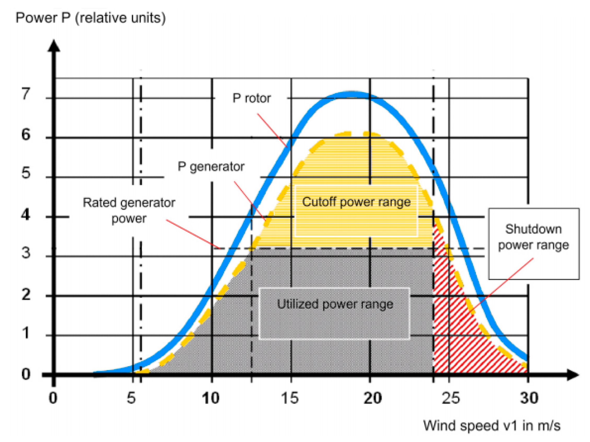
Energies 14 06798 g001
Figure 2. Control regions of blade-angle controller.
Energies 14 06798 g002
Figure 3. (a) Connection diagram of wind power plant. (b) Laboratory setup of wind power plant.
Energies 14 06798 g003
Figure 4. (a) Active power responses for different blade angles at 5 m/s wind speed. (b) Active power responses for different blade angles at 6 m/s wind speed. (c) Active power responses for different blade angles at 7 m/s wind speed.
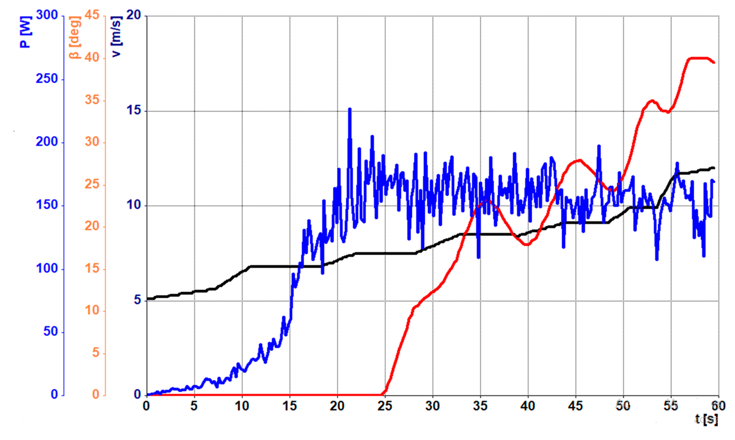
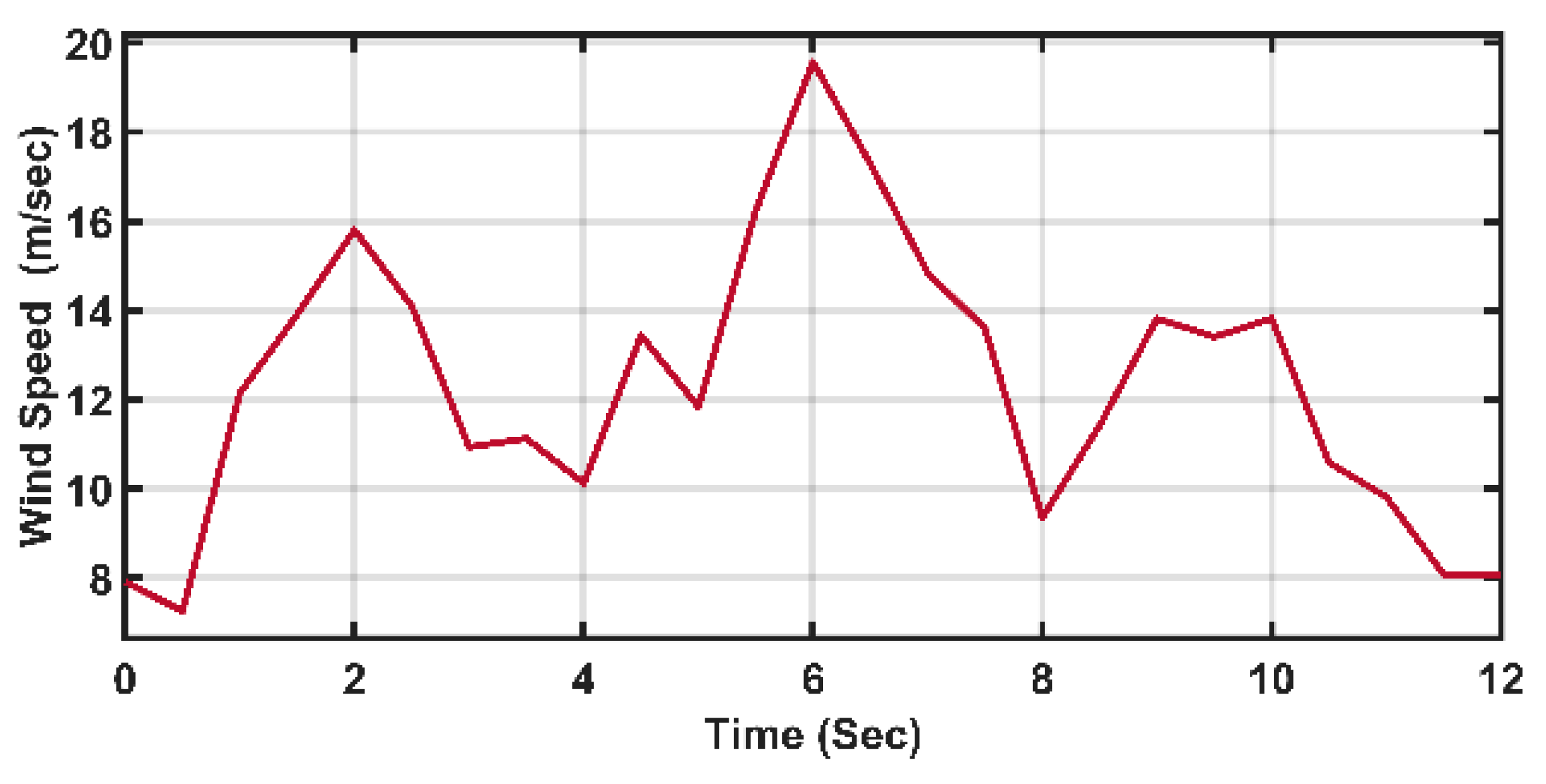
Energies 14 06798 g004
Figure 5. Wind speed, active power, and blade angle of first experimental case study.
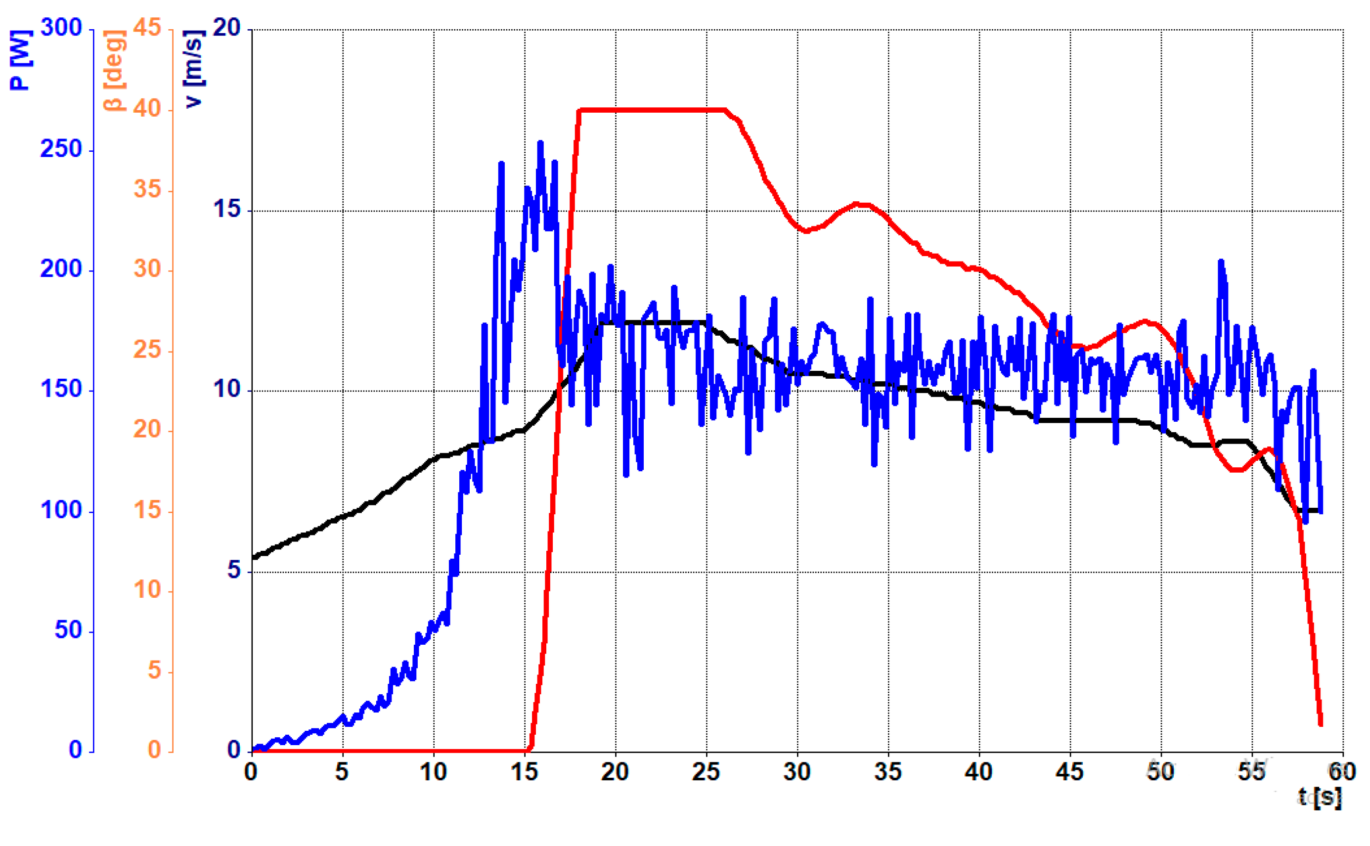
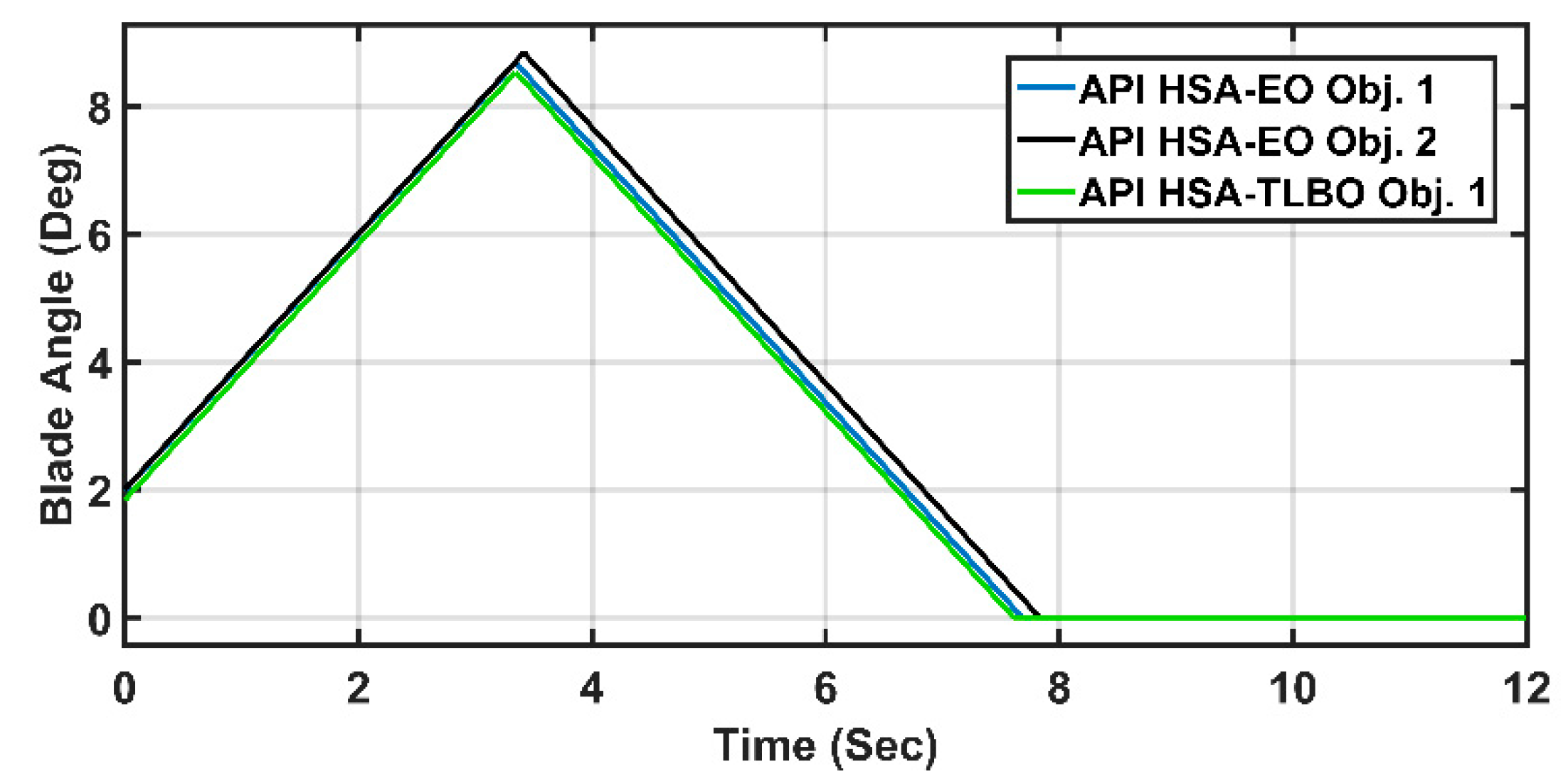
Energies 14 06798 g005
Figure 6. Wind speed, active power, and blade angle of second experimental case study.
Energies 14 06798 g006
Figure 7. Wind speed, active power, and blade angle of third experimental case study.
Energies 14 06798 g007
Figure 8. Wind speed, active power, and blade angle of fourth experimental case study.
Energies 14 06798 g008
Figure 9. MATLAB model of wind-turbine DFIG.
Energies 14 06798 g009
Figure 10. Block diagram representation of the adaptive PI controller.
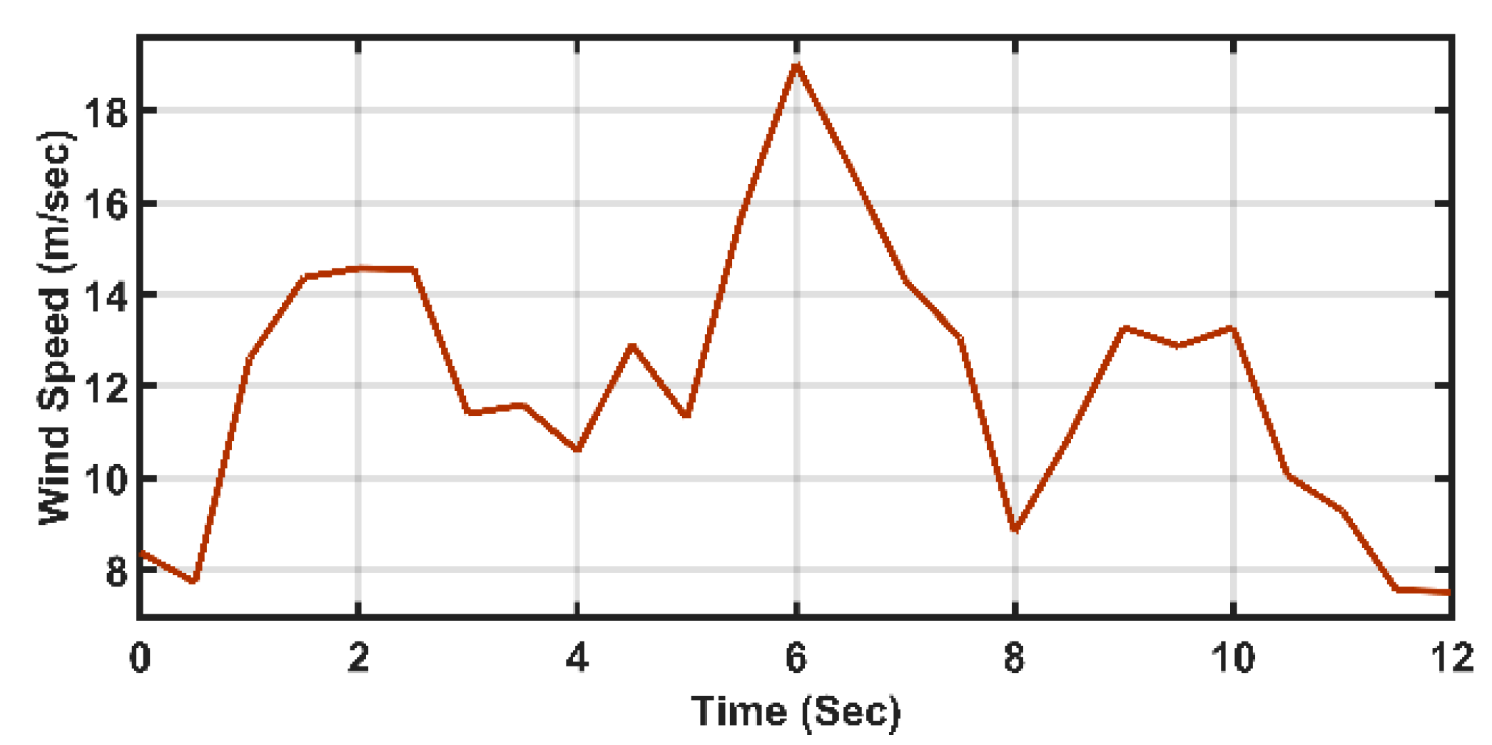
Energies 14 06798 g010
Figure 11. Wind-speed profile of normal first case.
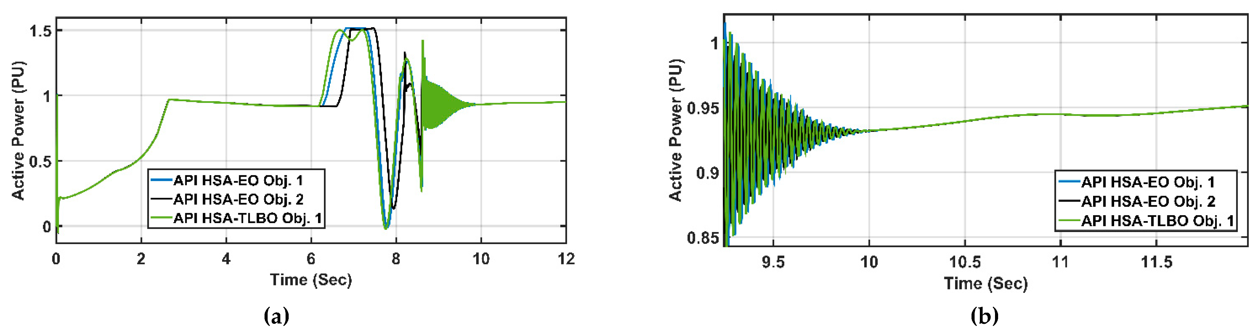
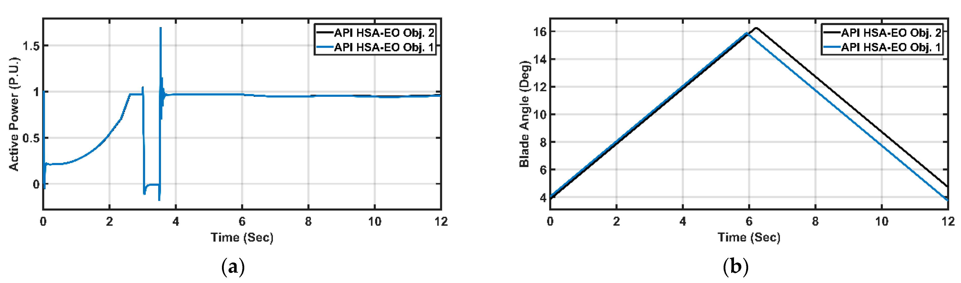
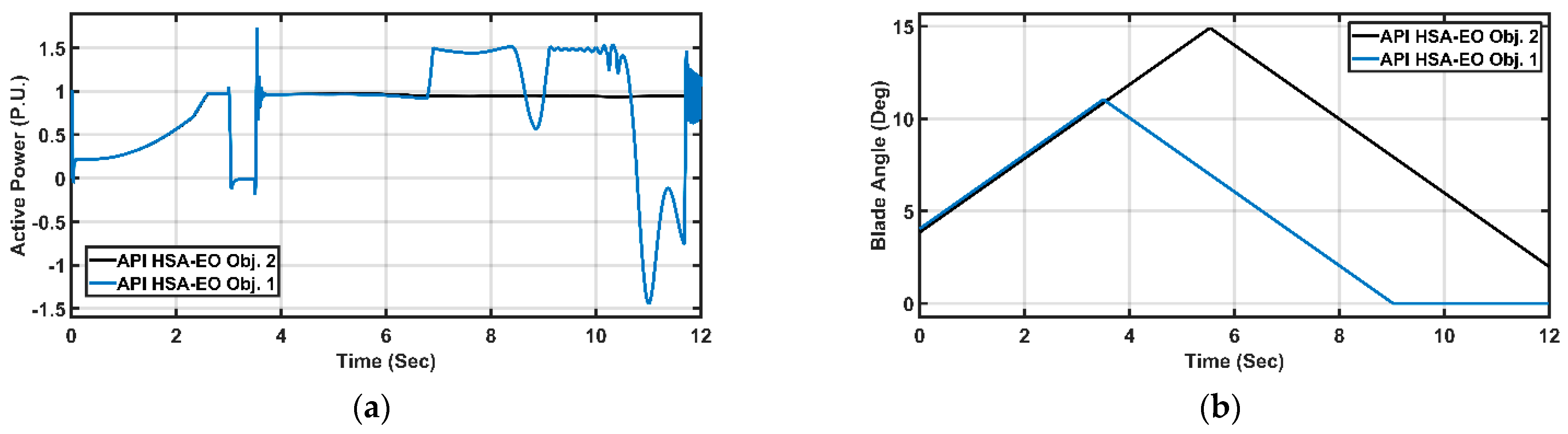
Energies 14 06798 g011
Figure 12. (a) Active power responses of normal first case. (b) Focusing of the active power response. (c) Blade−angle responses of normal first case.
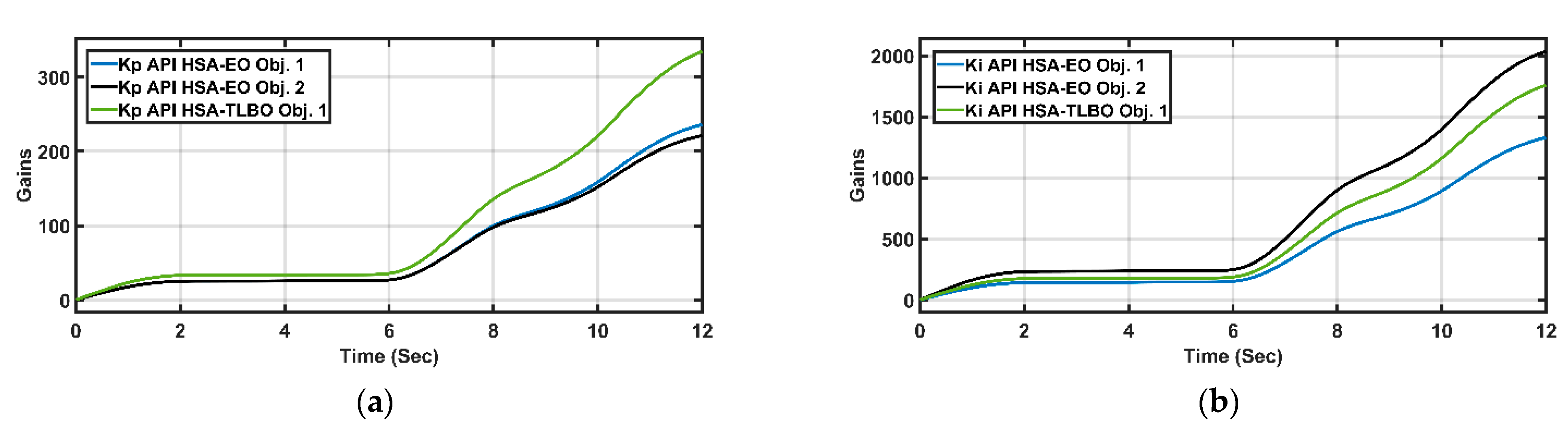
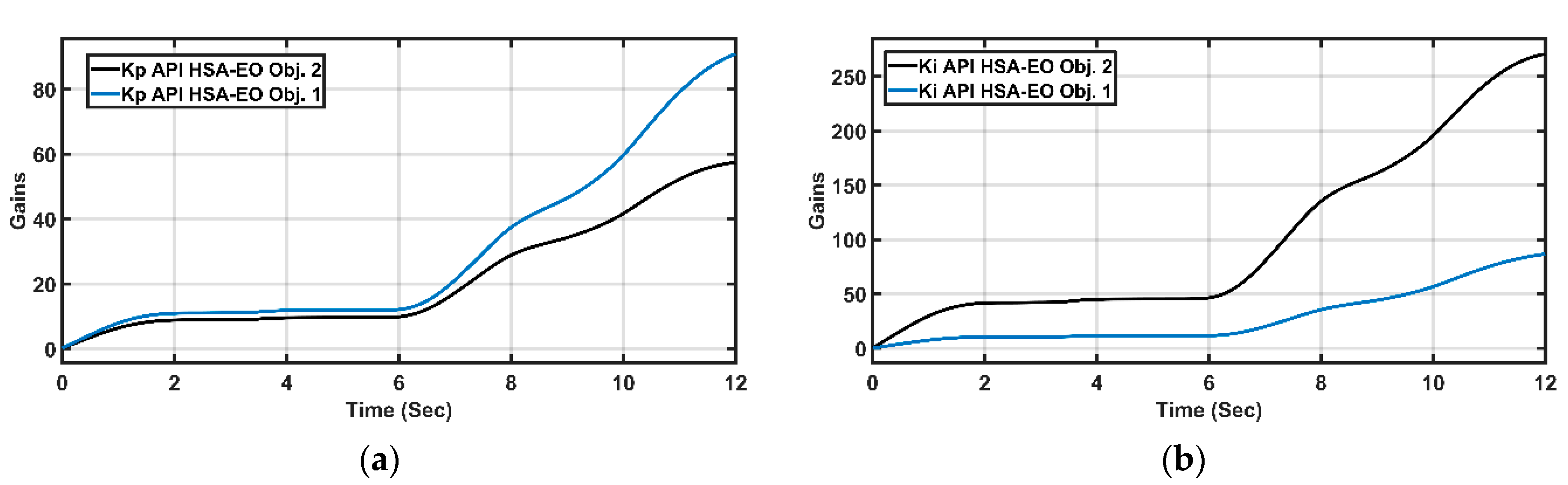
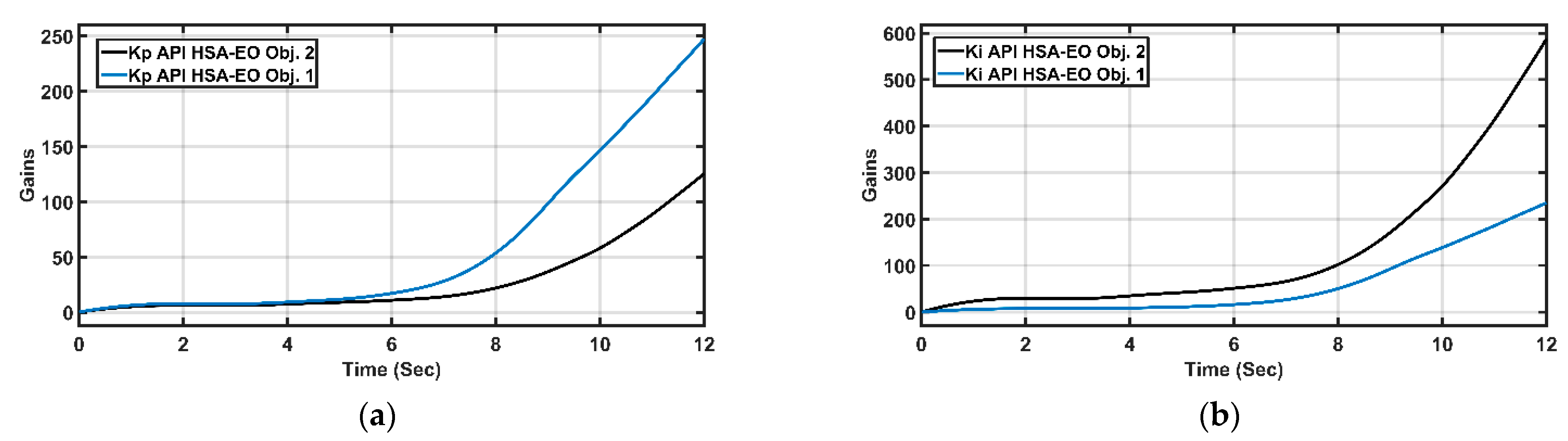
Energies 14 06798 g012
Figure 13. (a) K p adaptive PI gain of normal first case. (b) K i adaptive PI gain of normal first case.
Energies 14 06798 g013
Figure 14. Total harmonic distortion (THD) percentage of the four controllers under normal operation.
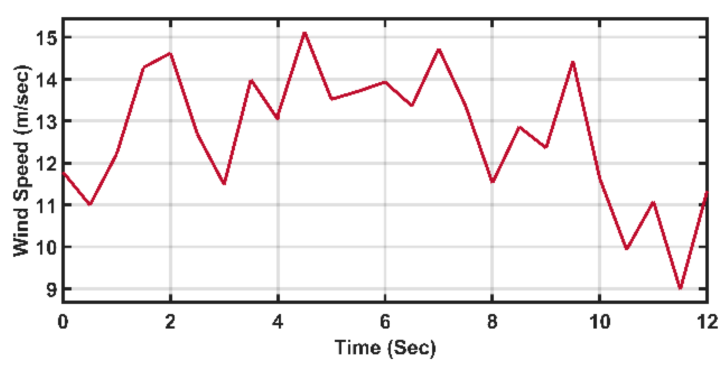
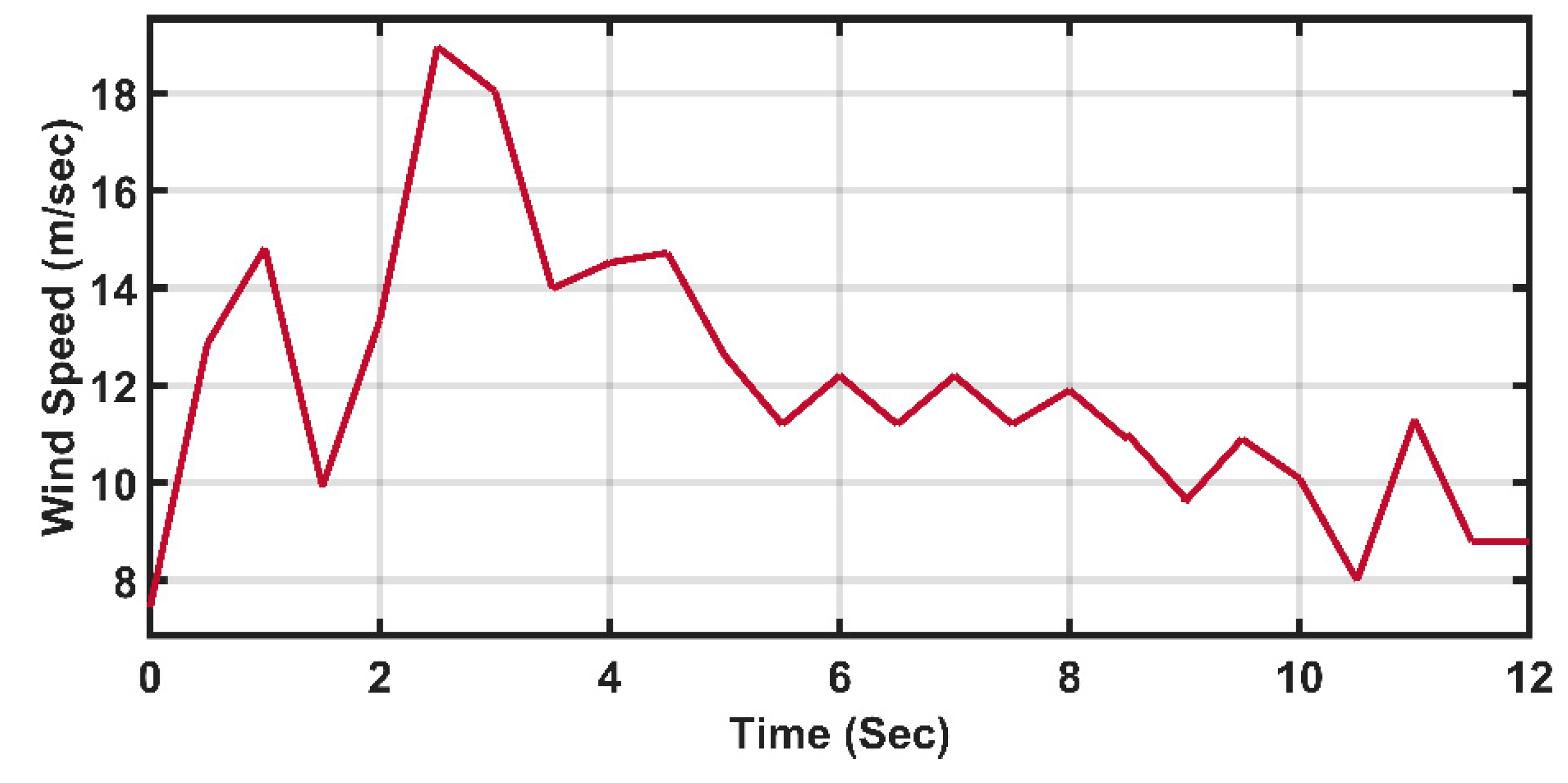
Energies 14 06798 g014
Figure 15. Wind-speed profile of normal second case.
Energies 14 06798 g015
Figure 16. (a) Active power responses of normal second case. (b) Blade-angle responses of normal second case.
Energies 14 06798 g016
Figure 17. (a) K p adaptive PI gain of normal second case. (b) K i adaptive PI gain of normal second case.
Energies 14 06798 g017
Figure 18. The wind-speed profile of normal third case.
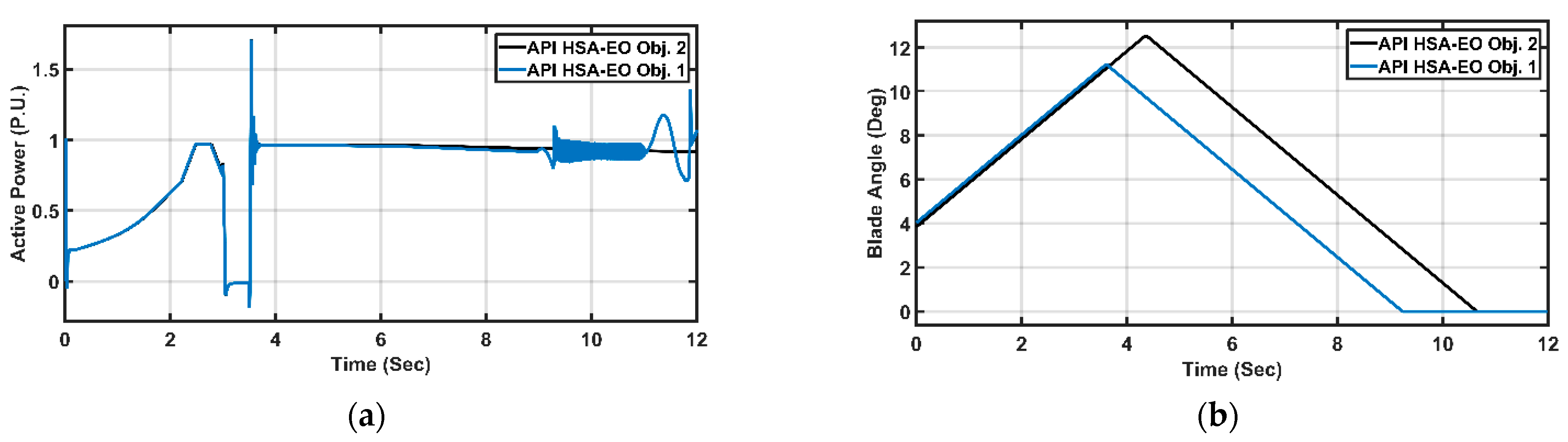
Energies 14 06798 g018
Figure 19. (a) Active power responses of normal third case. (b) Focusing active power responses of normal third case.
Energies 14 06798 g019
Figure 20. (a) Blade-angle responses of normal third case. (b) K p adaptive PI gain of normal third case. (c) K i adaptive PI gain of normal third case.
Energies 14 06798 g020
Figure 21. Wind-speed profile of normal fourth case.
Energies 14 06798 g021
Figure 22. (a) Active power responses of normal fourth case. (b) Focusing active power responses of normal fourth case.
Energies 14 06798 g022
Figure 23. Blade angle of the controllers at normal fourth case.
Energies 14 06798 g023
Figure 24. (a) K p adaptive PI gain of normal second case. (b) K i adaptive PI gain of normal second case.
Energies 14 06798 g024
Figure 25. (a) Active power responses of faulty first case. (b) Blade-angle responses of faulty first case.
Energies 14 06798 g025
Figure 26. (a) K p adaptive PI gain of faulty first case. (b) K i adaptive PI gain of faulty first case.
Energies 14 06798 g026
Figure 27. THD percentage of the two controllers under faulty operation.
Energies 14 06798 g027
Figure 28. Wind-speed profile of faulty second case.
Energies 14 06798 g028
Figure 29. (a) Active power responses of faulty second case. (b) Blade-angle responses of faulty second case.
Energies 14 06798 g029
Figure 30. (a) K p adaptive PI gain of faulty second case. (b) K i adaptive PI gain of faulty second case.
Energies 14 06798 g030
Figure 31. Wind-speed profile of faulty third case.
Energies 14 06798 g031
Figure 32. (a) Active power responses of faulty third case. (b) Blade-angle responses of faulty third case.
Energies 14 06798 g032
Figure 33. (a) K p adaptive PI gain of faulty third case. (b) K i adaptive PI gain of faulty third case.
Energies 14 06798 g033
Figure 34. Wind-speed profile of faulty fourth case.
Energies 14 06798 g034
Figure 35. (a) Active power responses of faulty fourth case. (b) Blade-angle responses of faulty fourth case.
Energies 14 06798 g035
Figure 36. (a) K p adaptive PI gain of faulty third case. (b) K i adaptive PI gain of faulty third case.
Energies 14 06798 g036
Table 1. Controller parameters in normal operation.
CONTROLLERSParameters
PID HSA Obj. 1 [39] K P K i K d
6813.772
API HSA Hybrid TLBO Obj. 1 [40] K 1 K 2 K c
155.25817.5426.63
API HSA-EO Obj. 111766028.83
API HSA-EO Obj. 21171078.229
Table 2. Numerical comparison between the controllers at normal first case.
ControllersRising TimeSettling TimePositive PeakNegative Peak
PID2.05 s9 s1.51 pu−0.85 pu
API HSA-TLBO2.72 s5.35 s0.975 pu−0.625 pu
API HSA-EO Obj. 12.715 s5.34 s0.975 pu−0.619 pu
API HSA-EO Obj. 22.714 s5.34 s0.975 pu−0.619 pu
Table 3. Statistical analysis of the active power—normal first case.
ControllersStandard Deviation (SD)Root Mean Square Error (RMSE)
PID0.4039 0.4447
API HSA-TLBO0.3245 0.4293
API HSA-EO Obj. 10.32430.4205
API HSA-EO Obj. 20.3268 0.4205
Table 4. Numerical comparison between the controllers at normal second case.
ControllersRising TimeSettling TimePositive PeakNegative Peak
API HSA-TLBO2.45 s2.45 s0.975 pu0.975 pu
API HSA-EO Obj. 12.45 s10.9 s0.975 pu0.667 pu
API HSA-EO Obj. 22.45 s2.45 s0.975 pu0.975 pu
Table 5. Statistical analysis of the active power—normal second case.
ControllersSDRMSE
API HSA-TLBO0.32970.4044
API HSA-EO Obj. 10.32070.3965
API HSA-EO Obj. 20.32510.3961
Table 6. Numerical comparison between the controllers at normal third case.
ControllersRising TimeSettling TimePositive PeakNegative Peak
API HSA-TLBO2.445 s12 s1.515 pu−0.355 pu
API HSA-EO Obj. 12.435 s11.4 s1.515 pu0.081 pu
API HSA-EO Obj. 22.435 s11.1 s1.515 pu0.188 pu
Table 7. Statistical analysis of the active power—normal third case.
ControllersSDRMSE
API HSA-TLBO0.37180.4143
API HSA-EO Obj. 10.3610.4013
API HSA-EO Obj. 20.34490.3868
Table 8. Numerical comparison between the controllers at normal fourth case.
ControllersRising TimeSettling TimePositive PeakNegative Peak
API HSA-TLBO2.66 s10.035 s1.501 pu−0.02 pu
API HSA-EO Obj. 12.65 s10.005 s1.515 pu−0.01 pu
API HSA-EO Obj. 22.65 s10.005 s1.515 pu0.133 pu
Table 9. Statistical analysis of the active power—normal fourth case.
ControllersSDRMSE
API HSA-TLBO0.33030.3658
API HSA-EO Obj. 10.33180.3642
API HSA-EO Obj. 20.3170.3487
Table 10. Controller parameters used in faulty operation cases.
ControllersParameters
K1K2Kc
API HSAEO Obj. 150.83048.53858.551
API HSAEO Obj. 241193.56855.838
Table 11. Numerical comparison between the controllers at faulty first case.
ControllersRising TimeSettling TimePositive PeakNegative Peak
API HSA-EO Obj. 12.65 s3.81 s1.69 pu−0.185 pu
API HSA-EO Obj. 22.65 s3.81 s1.69 pu−0.185 pu
Table 12. Statistical analysis of the active power—faulty first case.
ControllersSDRMSE
API HSA-EO Obj. 10.39660.4962
API HSA-EO Obj. 20.39430.4922
Table 13. Numerical comparison between the controllers at faulty second case.
ControllersRising TimeSettling TimePositive PeakNegative Peak
API HSA-EO Obj. 12.49 s12 S1.71 pu−0.188 pu
API HSA-EO Obj. 22.49 s3.81 S1.71 pu−0.188 pu
Table 14. Statistical analysis of the active power—faulty second case.
ControllersSDRMSE
API HSA-EO Obj. 10.32140.3785
API HSA-EO Obj. 20.37810.4759
Table 15. Numerical comparison between the controllers at faulty third case.
ControllersRising TimeSettling TimePositive PeakNegative Peak
API HSA-EO Obj. 12.605 s12 s1.725 pu−1.439 pu
API HSA-EO Obj. 22.605 s3.81 s1.725 pu−0.191 pu
Table 16. Statistical analysis of the active power—faulty third case.
ControllersSDRMSE
API HSA-EO Obj. 10.596 0.6236
API HSA-EO Obj. 20.4001 0.5040
Table 17. Numerical comparison between the controllers at faulty fourth case.
ControllersRising TimeSettling TimePositive PeakNegative Peak
API HSA-EO Obj. 12.615 s10.3 s1.910 pu−0.234 pu
API HSA-EO Obj. 22.615 s10.1 s1.915 pu−0.232 pu
Table 18. Statistical analysis of the active power—faulty fourth case.
ControllersSDRMSE
API HSA-EO Obj. 10.4226 0.4568
API HSA-EO Obj. 20.3859 0.4291
Publisher’s Note: MDPI stays neutral with regard to jurisdictional claims in published maps and institutional affiliations.

