1. Introduction
Gold is not only a consumption good, but also a good for investment, especially during severe financial distress when the values of many assets drop sharply but the gold price increases. This is because gold is a well-established safe haven [
1]. In other words, investors often turn to gold because it potentially offers portfolio diversifications and hedging benefits during periods of turmoil in conventional financial markets. Silver and platinum, in contrast, are precious metals with similar consumption-based uses as gold. Therefore, the gold-to-silver and gold-to-platinum price ratios should be largely unaffected by consumption (jewelry demand) shocks, and hence variations should reveal variations in risk, implying that the two ratios could serve as alternative proxies for a key economic state variable [
2,
3,
4].
Given this hypothesis, the objective of our research is to analyze the forecastability of the volatility of oil-price movements, as measured by monthly realized variance (
RV), based on the information content of gold-to-silver and gold-to-platinum price ratios, by undertaking a historical analysis of the monthly West Texas Intermediate (WTI) oil price over the periods 1915:01–2021:03 and 1968:01–2021:03, respectively. It should be noted that [
2,
3,
4] dealt with the forecasting of excess aggregate and industry-level stock returns, and bond premia in the United States (US), using the gold-to-platinum price ratio. Here, we not only look at the gold-to-platinum price ratio but also add the gold-to-silver price ratio for forecasting oil
RV, given that silver shares similar properties with platinum from the perspective of consumption.
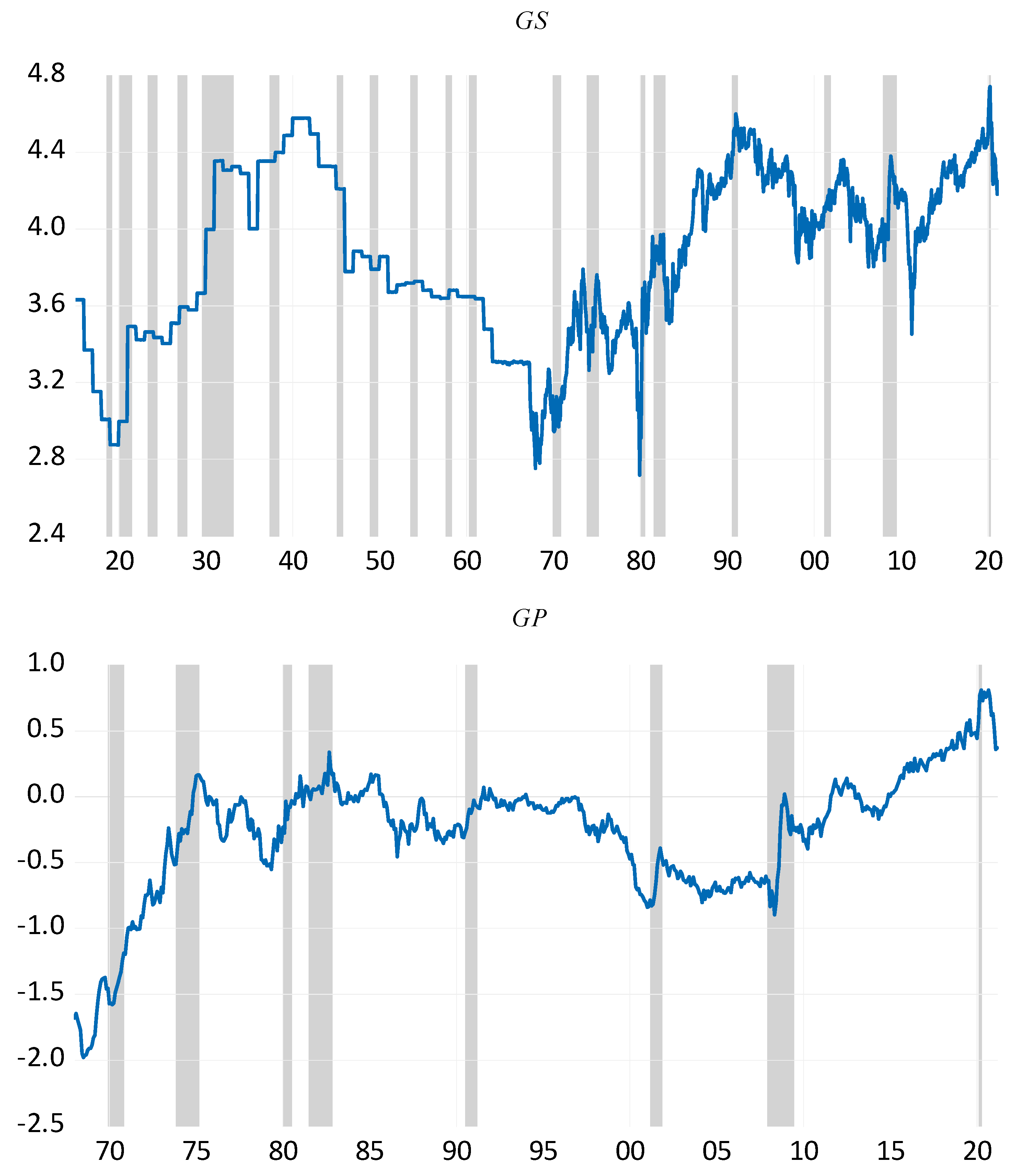
Intuitively, higher gold-to-silver and gold-to-platinum price ratios signal increased risks in financial markets, which, in turn, would suggest deteriorating economic conditions [
5], as seen in
Figure A1 in the
Appendix A. One can observe from the figure that the two ratios increased before every major National Bureau of Economic Research (NBER)-based economic recession in the US, as shown by the shaded months. The ratios also had an upward trend during the recent US-China trade war that started in 2016 (and also the Brexit negotiations), which resulted in a slowdown of the global economy. This finding is not surprising, since a common view is that the US-China trade war has made the world a riskier place (risk is commonly viewed as that type of uncertainty which rational agents face when making their decisions: even though the agents can contemplate all possible states of nature and their likelihood, the exact realization is not known [
6]; that is, risk is characterized by situations where one knows the odds of the unknown or the probability distribution of stochastic events). Economic theory suggests that more uncertain prospects for international trade have the potential to affect the economic decisions of households and firms. For example, [
7] argues that an agent’s decision-making is influenced by uncertainty because uncertainty raises the option value of waiting. Real options theory generally explains the negative impact of uncertainty on economic activity. In other words, uncertainty makes economic agents more cautious, due to the high cost of making the wrong investment decision (due to irreversibility), and as a result they postpone investment, hiring, and consumption (of durable goods) decisions. This then results in cyclical fluctuations of macroeconomic aggregates. At the same time, oil-price volatility is known to be countercyclical, due to the fact that oil-price increases (decreases) associated with higher (lower) demand due to expansions (recessions) are considered to be good (bad) news for the oil market, and hence reduce (increase) oil-market volatility [
8,
9,
10]. This reasoning is based on the intuition that higher global risks tend to make the path of the future aggregate demand of oil (and commodities in general) and, as a result, aggregate production, less predictable [
11]. The ‘theory of storage’ [
12,
13] outlines the increased volatility of commodity prices resulting from a rise in convenience yield, as risk-averse oil (commodity) producers prefer to hold physical stock. Naturally, higher global risk, reflected by the higher gold-to-silver and gold-to-platinum ratios, resulting in US recessions or downturns, will produce large oil-price fluctuations. In summary, we can hypothesize that the
RV of oil-price movements is positively linked to these two ratios.
To the best of our knowledge, this is the first paper to use gold-to-silver and gold-to-platinum price ratios for forecasting the
RV of oil-price movements (that is, returns) using a century and a half of historical data. We must emphasize that using
RV (calculated by taking the sum of squared daily returns over a month) following [
14] to measure volatility, an otherwise latent process, provides us with an observable and unconditional metric of volatility, as opposed to using generalized autoregressive conditional heteroscedasticity (GARCH), including the numerous variants of GARCH models discussed in the existing literature such as, for example, EGARCH models and multivariate GARCH models (see, for example, [
15,
16]) or stochastic volatility (SV) models. By considering the role of gold-to-silver and gold-to-platinum ratios as proxies for global risk, our paper adds to the vast existing literature on the forecastability of oil-returns volatility based on a wide array of models and predictors, including macroeconomic, financial, behavioral, and climate-patterns-related predictors (for detailed reviews, see [
17,
18,
19,
20]). We also note that by considering the longest possible monthly data spans for relating these two ratios to the oil
RV, we avoid the issue of sample selection bias in our analysis. We must also emphasize that the objective of our paper is not to make a methodological contribution, but to introduce two metrics of global risk when forecasting the longest possible datasets for oil-market volatility, using standard models available in the literature.
Accurate forecasting of oil-returns volatility has important implications for both investors and policymakers. The authors of [
21] note that volatility, interpreted as uncertainty, becomes a key input to investment decisions and portfolio allocation; hence, the ability to precisely forecast oil-returns volatility is of paramount importance for oil traders, especially in the wake of the recent financialization of the oil market [
22]. Moreover, oil-returns volatility has been associated with a negative impact on global economic activity [
23], and thus forecasts of the future path of oil-returns volatility also provide key information for policymakers who are responsible for developing monetary and fiscal policies.
The remainder of the paper is organized as follows:
Section 2 describes the data and methodology,
Section 3 discusses the forecasting results, and
Section 4 concludes the paper.
2. Data and Methodologies
The data we used for our analysis were daily and monthly WTI crude oil spot prices, obtained from Global Financial Data (
https://globalfinancialdata.com/ (accessed on 1 July 2021)), with the start and end dates determined by the availability of the data for the predictors at the time of writing this paper. For both the daily and monthly frequencies of the oil-price data, we calculated the first difference of the price and then multiplied it by 100 to obtain log returns in percentages. Then, the
RV was computed as the sum of daily squared returns over a month, as per the availability of daily data. It should be noted that oil-price data were available at a monthly frequency only over the period 1920–1976, and hence, we measured
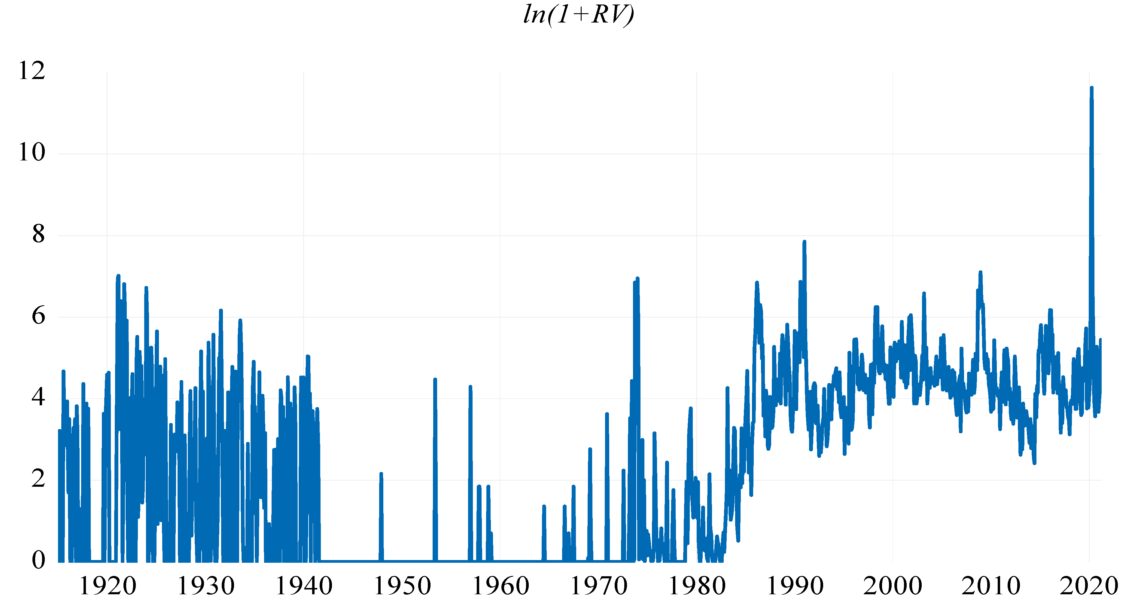
RV as the monthly squared log-returns over these parts of the overall sample. We conducted the forecasting analysis using
= ln(1 +
RV) for all t, rather than modelling
RV directly, because the latter method exhibits a very large peak at the end of the sample period, associated with the outbreak of the COVID-19 pandemic.
Following [
24], we initially specified a heterogenous autoregressive (HAR)-RV model, which included one lag each of the averages of
over a quarter and a year, but the corresponding coefficients were insignificant, and hence we used the specification in Equation (1).
The forecasting model of
used is given by:
where
is the realized volatility at time
t and
is the average value of
over
t + 1 to
t + h, where
h represents the five forecasting horizons considered in our paper, i.e., 1, 3, 6, 9, and 12 months ahead.
Ratiost is the ratio of either gold-to-silver prices or gold-to-platinum prices in their natural-logarithmic form, and acts as a proxy for risk at time
t, and
is the disturbance term. Our benchmark model is nested in Equation (1) and obtained by setting
γ = 0.
The nominal gold and silver prices in US dollars were derived from Macrotrends (
https://www.macrotrends.net/ (accessed on 1 July 2021)) while the nominal platinum price was obtained from Kitco (
https://www.kitco.com/ (accessed on 1 July 2021)). The nominal gold- and silver-price data started from 1915:01, and that month defines the starting point of the analysis involving the logarithmic value of the gold-to-silver price ratio (
GSt). Because platinum data were only available from 1968:01 onward, the analysis associated with the logarithm of the gold-to-platinum price ratio (
GPt) was conducted over a shorter sample period beginning at that month. Our analyses ended in 2021:03, which was the last available data point for all our variables at the time of writing this paper.
Figure A1 (
Appendix A) plots the variables of concern, i.e.,
,
GS, and
GP, with the latter two superimposed on the recession dates of the US. All these three variables were found to be stationary, based on standard unit root tests (i.e., without incorporating breaks), with complete details of these results available upon request from the authors.
3. Empirical Results
We focused our predictive analysis on the out-of-sample performance of our models, as [
25] notes that this is the ultimate test of any predictive model (in terms of the econometric methodologies and predictors employed). However, for the sake of completeness, the full-sample estimation results of Equation (1) for both
Ratios and for
h = 1, 3, 6, 9, and 12, with [
26] heteroscedasticity and autocorrelation-adjusted (HAC) standard errors, are provided in
Table 1. We find that both these precious-metals ratios consistently increase
RV in a statistically significant manner (at the 1% significance level when we use
GS and at the 5% significance level when we use
GP) for all five forecasting horizons considered. This finding is in line with the intuition outlined in the Introduction, which pointed out that increases in
GS or
GP are indicative of higher risk and lower economic activity, which, in turn, increases the oil-price volatility due to its countercyclical nature.
Based on the suggestion of an anonymous referee, we also conducted linear Granger tests of causality and found statistically significant evidence of in-sample predictability at the 1% and 5% levels, respectively, under
GS and
GP, with no feedback from
. In addition, impulse response analysis, with the structural shocks identified using Cholesky decomposition, i.e., with
GS or
GP ordered first in the VAR, showed that shocks to these two predictors affect
in a positive and significant manner over the entire one-year-ahead forecast horizon, in line with the data reported in
Table 1. A variance decomposition analysis showed that the ability of
GS and
GP to explain the variability in
increased over the one- to twelve-month-ahead forecast horizon, and
GS explains 2.3613% of the variation in
on average, while the corresponding figure is 2.2251% for
GP. Complete details of these results are available upon request from the authors.
In order to conduct the forecasting exercise, we first determined the in- and out-of-sample split, based on the [
27] tests of multiple structural breaks applied to Equation (1) under
GS and
GP for
h = 1, 3, 6, 9, and 12 months ahead. The tests detected 5 breaks in each of the 10 cases, with the earliest structural change detected in 1935:08 and 1976:01 for
GS and
GP, respectively (complete details of the structural break dates are available upon request from the authors). Therefore, our in-sample periods covered 1915:01–1936:07 and 1968:01–1975:12, and the out-of-sample periods were 1936:08–2021:03 and 1976:01–2021:03 for
GS and
GP, respectively. Our forecasting models with and without the two ratios were estimated recursively over their respective out-of-sample periods, which ensured that the changes in the parameter estimates of the model due to all other breaks that existed over the forecasting sample were accounted for.
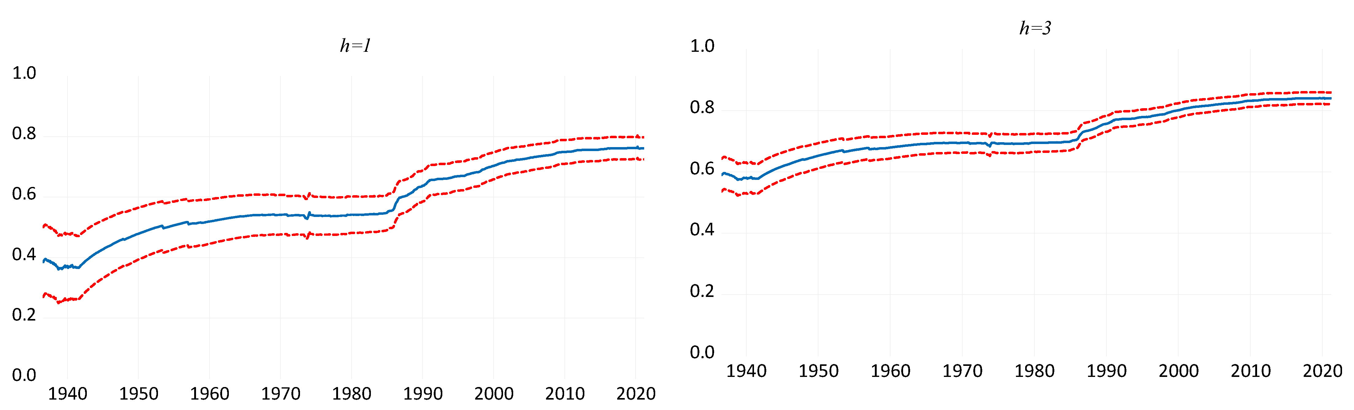
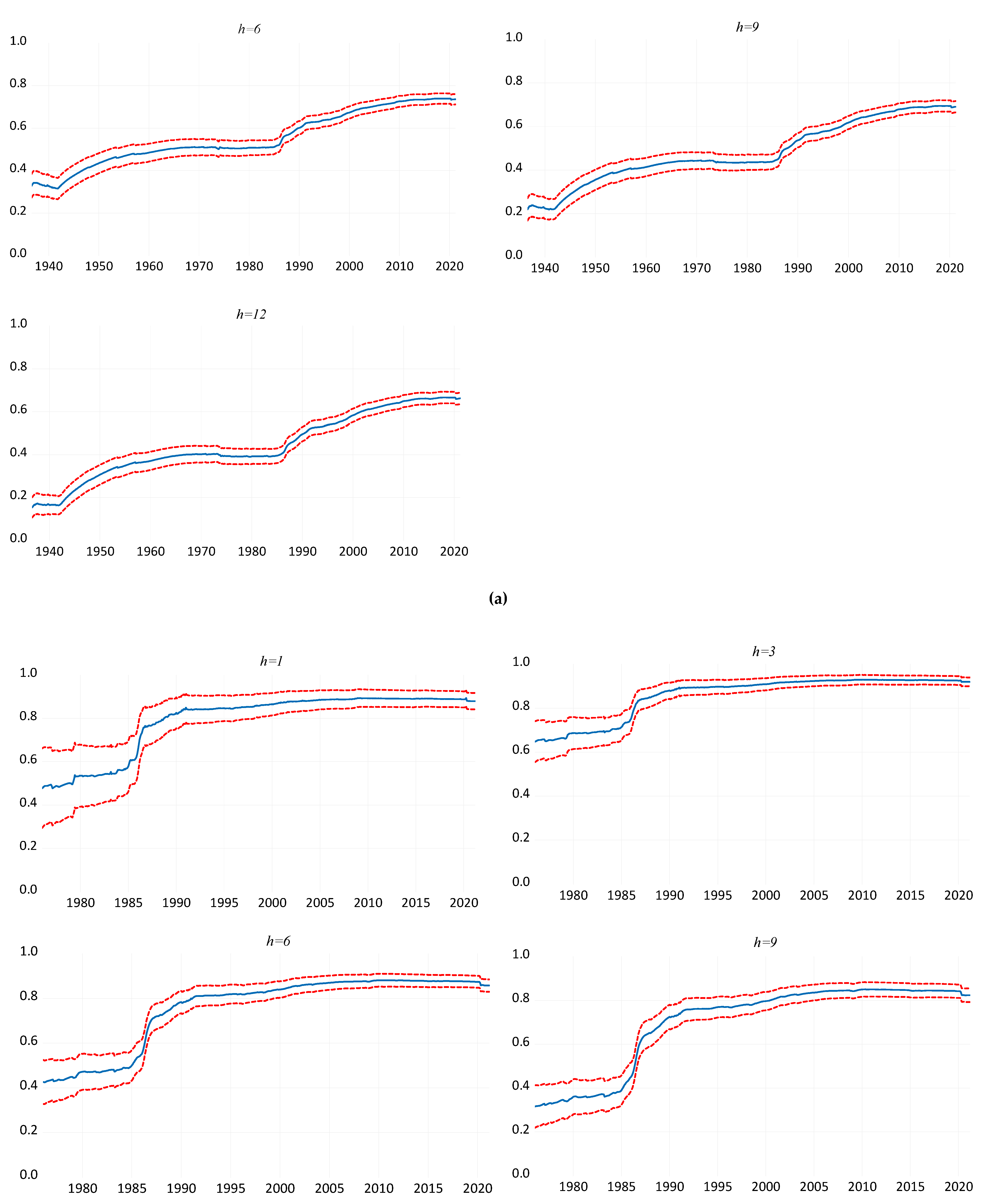
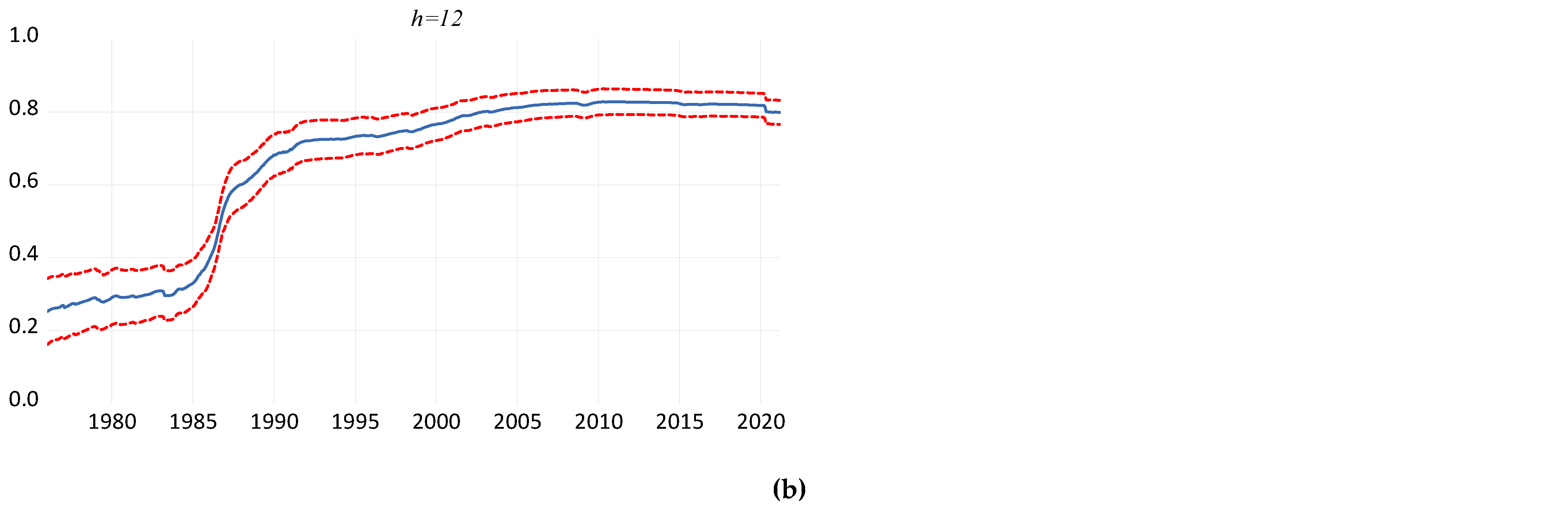
As suggested by an anonymous referee, in order to track the evolution of the effects of
GS and
GP on
, we plotted the recursive estimates of
γ corresponding to
GS and
GP, respectively, over the corresponding out-of-sample periods for
h = 1, 3, 6, 9, and 12, as shown in
Figure A2a,b in the
Appendix A. As shown in the plots, the effects of
GS and
GP on
over the relevant out-of-sample periods were not only consistently positive and statistically significant but also increased in strength over time.
Table 2 presents the ratio of mean-squared forecast errors (MSFEs) for the unrestricted model with
GS or
GP and the restricted model without the two ratios, for
h = 1, 3, 6, 9, and 12. It should be noted that
MSE-F = (
T − R − h + 1) (
MSFER − MSFEUR)/
MSFEUR, where
T is the sample size,
R is the length of the in-sample,
h is the forecast horizon, and
MSFER and
MSFEUR are
MSFEs from the restricted (benchmark) and unrestricted (with the
Ratio as predictor) models, respectively. A positive and significant
MSE-F statistic indicates that the unrestricted model forecasts are statistically superior to those of the restricted model. As can be seen, the relative MSFEs were less than one under both
GS and
GP for all five forecast horizons. This suggests that including information on the two proxies for global risks in the model produces lower forecast errors associated with
RV compared to the case when the ratios are excluded. More specifically, the forecasting gains from
GS were equal to 7.1713%, 8.2584%, 9.7727%, 10.2746%, and 10.2948% for
h = 1, 3, 6, 9, and 12, respectively. The corresponding values for
GP were: 6.9194%, 8.3239%, 9.3775%, 9.8184%, and 10.3285% for the same set of forecasting horizons. Note that the forecasting gains increased over the out-of-sample period as the horizon became longer, suggesting that as the information on global risks is incorporated into investment decisions over the horizon of one year, the accuracy of the predictions of oil-market volatility improve. This is probably because heightened risks affect the oil-market volatility via a reduction in investment and consumption, which takes time to feed into the business cycles, and hence is reflected more strongly at longer horizons involving
RV.
More importantly, using the
MSE-F test discussed in [
28], the forecasting gains derived from
GS or
GP at
h = 1, 3, 6, 9, and 12 months ahead were statistically significant at the 1% level, relative to the nested benchmark (which excludes the
Ratios). In summary, higher values of the ratios of the gold price to the silver and platinum prices can forecast accurately the volatility (increases) in the oil-price returns for short, medium, and long forecasting horizons in a statistically significant fashion.
Based on the recommendation of an anonymous referee, we aimed to obtain more detailed information about our results by re-conducting our forecasting exercise using quantiles-based estimation of Equation (1). The general quantile regression model in [
29] is as follows:
, where
and
are assumed to be independent, and derived from an error distribution
, such that:
, with the
-th quantile equal to 0
The coefficients of the
-th conditional quantile distribution are estimated as:
where
determines the relationship between the independent variable(s) and the
-th conditional quantile of the dependent variable, with
being the indicator function. The decision to use this approach emanated from the recent popularity of quantile-
RV models, given that such estimation goes beyond the conditional mean-type (ordinary least squares (OLS)) approach used above, and is more informative, since it provides an analysis of the entire conditional distribution of the dependent variable [
30]. In the process, we were able to gauge whether the forecasting gains reported in
Table 1 were specific to the conditional state of
RV, with the lower, median, and upper quantiles capturing low, normal, and high volatilities in the oil market, respectively. This could provide additional information to investors and policymakers when taking their respective decisions, enabling them to understand clearly whether the role of these two global risk proxies is important for specific parts of the conditional distribution of
RV or for its entirety. In the former case, clearly these agents would need to look for other predictors for predicting the specific states of
RV where the gold-to-silver and gold-to-platinum ratios do not produce forecasting gains.
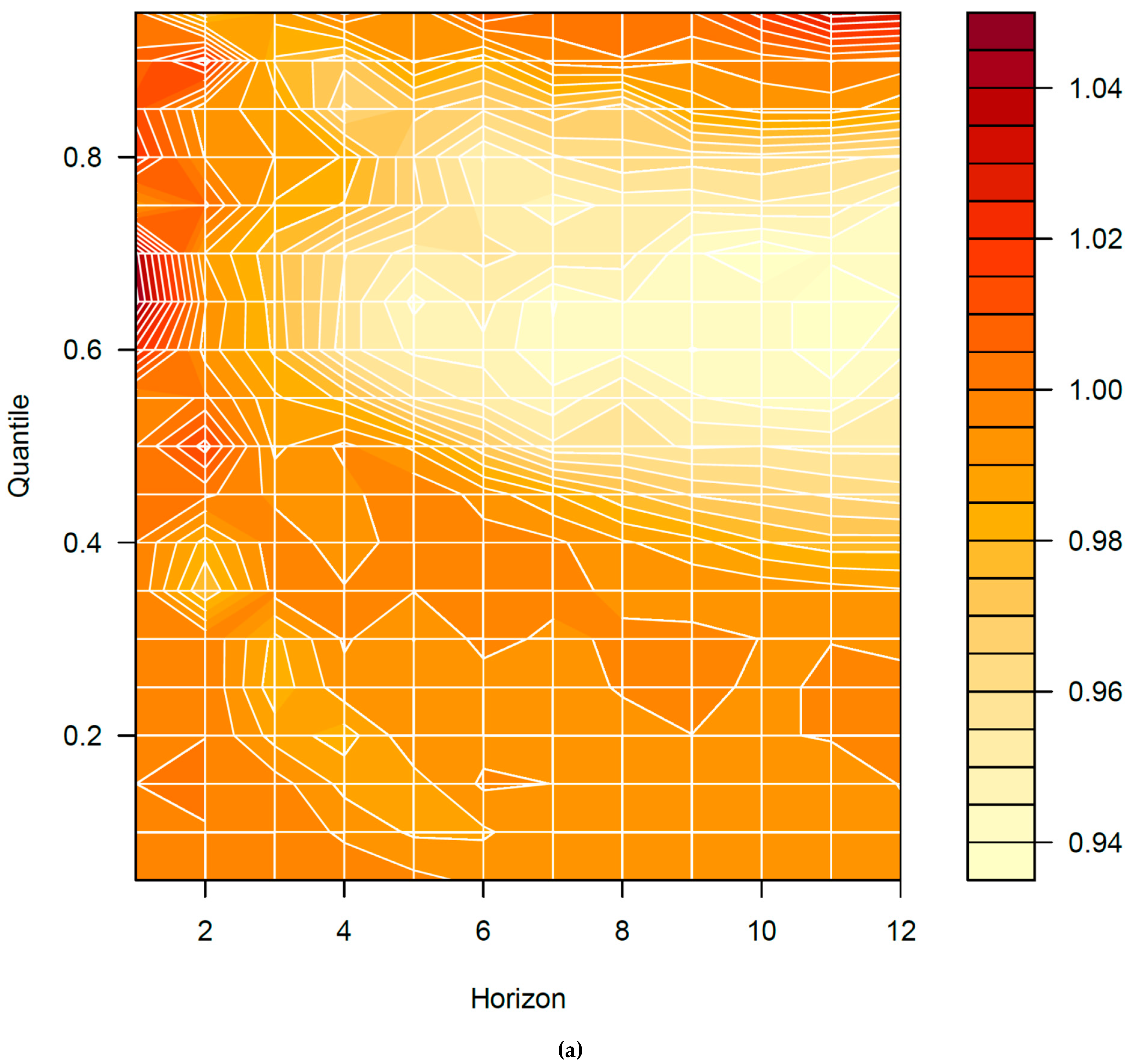
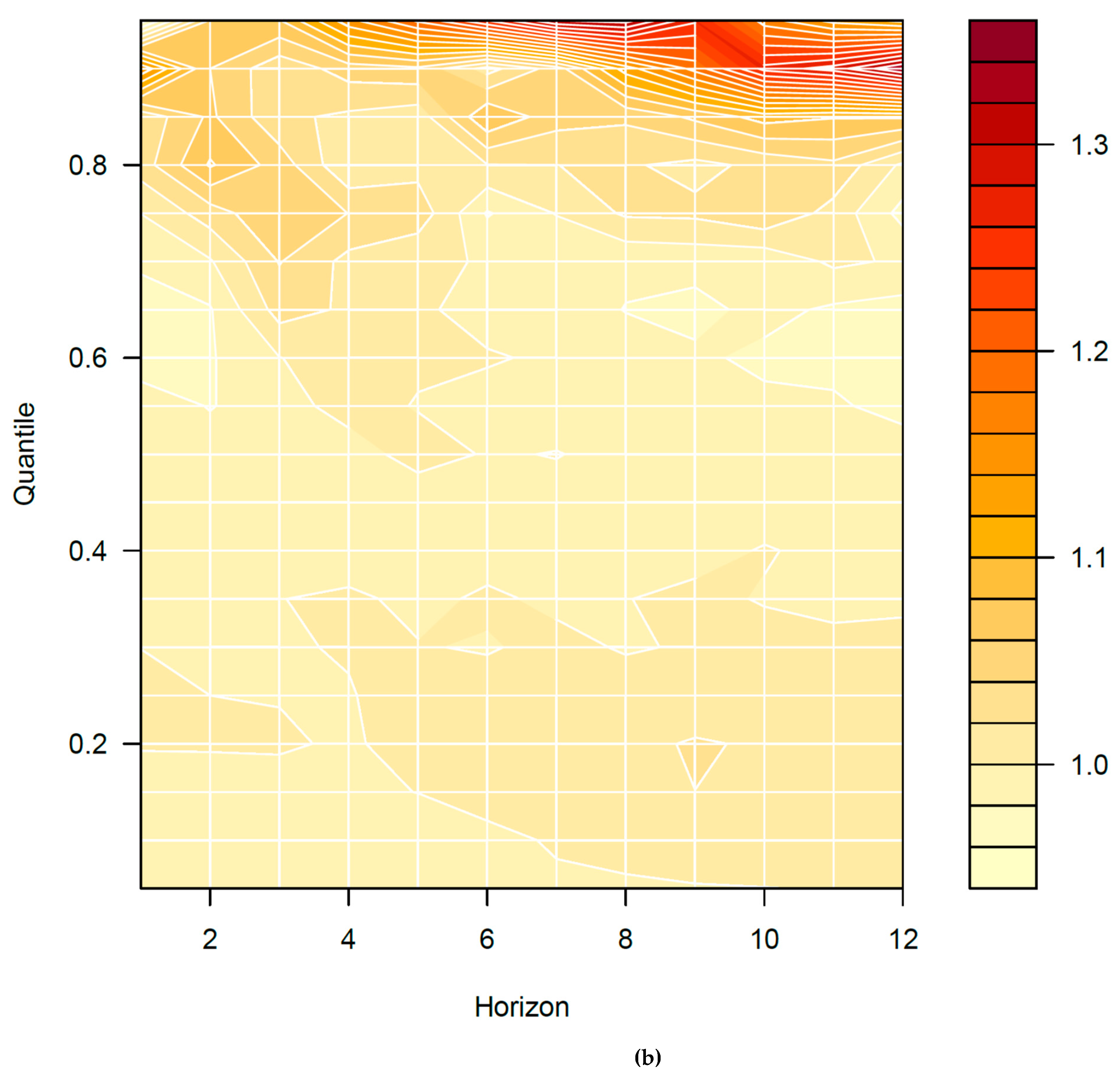
For this reason, we plotted the ratio of the MSFEs over the entire conditional distribution of the
RV due to GS and GP, respectively, derived under the same forecasting (i.e., in- and out-of-sample) setup as the conditional mean-based analysis, as shown in
Figure A3a,b in the
Appendix A. As shown the figures, in the case of GS, the ratio was virtually less than one for the entire conditional distribution of
RV, for forecast horizons larger than two months, with the strongest gains obtained around the median and moderately low and high quantiles. For GP, the range of combinations of forecast horizons and quantiles for which the ratios of MSFEs were less than one was smaller than for GS, but it was again centered around the median, becoming larger in terms of the quantile values for the short and long forecast horizons. That is, the best predictive performances of both GS and GP tended to be concentrated around the normal state of the
RV. Relatively weaker results at the two ends of the conditional distribution of
RV seem to suggest that, during extreme conditions of oil-market volatility, oil traders are likely to herd [
31], and hence do not require too much additional information from predictors over and above the past volatility. In other words, under very low- and high-volatility states of the oil market, investors and policymakers can just rely on the lagged volatility to predict the future path (or they may have to look for alternative predictors).
As an alternative metric of forecast performance, we used the check function underlying the quantile regression estimator as a loss function forecaster. To this end, we used the check function to compute the ratio of cumulated losses. Results showed that, in the case of GS, this ratio was less than one mainly for quantiles above the median, with the range of quantiles for which we observed ratios to be less than one increasing with the length of the forecast horizon. As for GP, the combinations of quantiles and forecast horizons yielding a ratio less than one were fragmented, with a center at quantiles above the median. Complete details of these results are available upon request from the authors.
4. Conclusions
We examined the predictive value of the (log) gold-to-silver and gold-to-platinum price ratios, which serve as proxies for risks, for the realized variance (RV) of oil-price movements (that is, returns) using monthly data for the sample periods 1915:01–2021:03 and 1968:01–2021:03. The results of an in-sample predictability analysis showed that these two ratios tend to increase RV in a statistically significant manner at all five forecasting horizons (h) of 1, 3, 6, 9, and 12 months ahead. We then turned to a forecasting analysis that is well established as a more powerful test of predictability, over the out-of-sample periods 1941:08–2021:03 and 1976:01–2021:03 for the gold-to-silver and gold-to-platinum price ratios (given the in-sample periods of 1915:01–1941:07 and 1968:01–1975:12), with the split being determined by structural break tests. From this setup, we found that statistically significant forecasting gains could be obtained from both these two ratios at short-, medium-, and long-term forecasting horizons, i.e., for h = 1, 3, 6, 9, and 12 months. In other words, in-sample evidence of predictability translates into predictability in the context of a forecasting experiment.
Our results have valuable implications for investors and policymakers as economic agents, given the importance of real-time forecasts of oil-price volatility for both investors and policy authorities. Policymakers in particular, could use our findings to obtain information on the future path of oil-price volatility due to global proxies of risks, as captured by the easy-to-calculate gold-to-silver and gold-to-platinum price ratios, in the short to long term. This knowledge, and the known negative impact of oil-price volatility on real economic activity, may be useful in anticipating economic recessions and designing appropriate monetary and fiscal policies for the stabilization or recovery of the macroeconomy. Moreover, as volatility is a key input in portfolio decisions, the forecastability of oil-price volatility due to the two precious-metals price ratios may be of vital importance to oil investors.
As an extension of this study, it would be interesting to investigate the role of these two ratios in predicting the volatility of other energy prices. To account for the effects of these two ratios on different frequency and time components of the volatility, one could use wavelet-based decomposition of the underlying returns data before computing RV, to obtain more detailed results.


