Article

Prediction of Extreme Conditional Quantiles of Electricity Demand: An Application Using South African Data

by
Norman Maswanganyi
1,†,
Caston Sigauke
2,*,† and
Edmore Ranganai
3,†
1
Department of Statistics and Operations Research, University of Limpopo, Private Bag X1106, Sovenga 0727, South Africa
2
Department of Statistics, University of Venda, Private Bag X5050, Thohoyandou 0950, South Africa
3
Department of Statistics, University of South Africa, Private Bag X6, Florida 1710, South Africa
*
Author to whom correspondence should be addressed.
These authors contributed equally to this work.
Energies 2021, 14(20), 6704; https://doi.org/10.3390/en14206704
Submission received: 12 May 2021 / Revised: 10 July 2021 / Accepted: 4 August 2021 / Published: 15 October 2021

Abstract

:
It is important to predict extreme electricity demand in power utilities as the uncertainties in the future of electricity demand distribution have to be taken into consideration to achieve the desired goals. The study focused on the prediction of extremely high conditional quantiles (between 0.95 and 0.9999) and extremely low quantiles (between 0.001 and 0.05) of electricity demand using South African data. The paper discusses a comparative analysis of the additive quantile regression model with an extremal mixture model and a nonlinear quantile regression model. The estimated quantiles at each level were then combined using the median approach. The comparisons were carried out using daily peak electricity demand data ranging from January 1997 to May 2014. Proper scoring rules were used to compare the three models, and the model with the smallest score was preferred. The results could be useful to system operators including decision-makers in power utility companies by giving insights and guidance for future electricity demand patterns. The prediction of extremely high quantiles of daily peak electricity demand could help system operators know the possible largest demand that will enable them to supply adequate electricity to consumers and shift demand to off-peak periods. The prediction of extreme conditional quantiles of daily peak electricity demand in the context of South Africa using additive quantile regression, nonlinear quantile regression, and extremal mixture models has not been performed previously to the best of our knowledge.

1. Introduction

In an attempt to diversify the energy mix, the South African government has developed a Renewable Energy Independent Power Producer Procurement Program (REIPPPP). The REIPPPP has proven to be a very successful program especially in bringing renewable energy projects to commercial operations over the past five years [1]. The country also came up with a new plan, namely the National Development Plan (NDP). The NDP is a plan for infrastructure development from 2013 to 2030. Moreover, the NDP is also an excellent guiding economic plan that set the GDP growth target per annum for the country to be able to meet its economic, social and political objectives [2].
In identifying the national goals relevant to establishing renewable energy policy objectives, South Africa needs to identify the key goals for the nation and how the electricity sector fits in among its priorities. The country also needs to take urgent actions to ensure the sustainability of renewable energy and energy efficiency by 2030. According to [3], renewable and energy efficiency have a positive impact on electricity demand during peak hours.
It is important to accurately predict extremely high quantiles of electricity demand. Uncertainties related to electricity demand have to be taken into account when predicting electricity demand. The superiority of extreme conditional quantile models over the least squares (conditional mean) model in the extremes of the conditional distribution is well established in the literature. Hence, accurate prediction of electricity demand at extreme levels could produce more useful information to decision-makers on the sustainability of renewable energy, energy generation and energy purchases. Furthermore, the accurate prediction of extreme electricity demand distributions would have a significant impact on mitigating load shedding and overloading and allow energy-efficient storage.
The main contribution of this paper is the use of additive quantile regression (AQR), extremal mixture (EM) and nonlinear quantile regression (NLQR) models in estimating the extremely high and extremely low quantiles of electricity demand using South African data. Such a study has not been carried out elsewhere to the best of our knowledge.
The highlights of the study are summarised as follows:
  • The study carried out a comparative analysis of EM, AQR and NLQR models in predicting extremely high and low daily peak electricity demand;
  • The identification of how electricity demand will change in the distribution networks in five to fifteen years going forward;
  • The prediction of extremely high quantiles of DPED could help system operators know the possible largest demand that will enable them to supply adequate electricity to consumers;
  • Knowing the possible largest demand of electricity at a given point in time can help system operators shift demand to off-peak periods.
The rest of the paper is structured as follows: Section 2 reviews several approaches proposed in the literature with some previous studies. Section 3 focuses on the semiparametric extremal mixture models, additive quantile regression model, nonlinear quantile regression model, and a brief explanation of the scoring rules. Section 4 presents the data used in the study including the exploratory data analysis. Section 5 gives a discussion of the results. Finally, the study is then concluded in Section 6.

2. Literature Review

Many statistical applications focus on either the lower or upper quantiles of the distributions. Consequently, the theory of extreme value techniques has been extensively used in many disciplines for the past several decades. The extremal quantile regression (EQR) model can also be utilised to model extreme values as an alternative to classical extreme value theory (EVT) techniques. EVT is widely used as a tool for risk management. Several estimators have been proposed for the estimation of extreme conditional quantiles, which include [4,5,6,7,8], among others. The literature has extensively dealt with EQR, which consists of one-stage and two-stage approaches. A study by [4] used a two-step procedure based on two case studies in estimating extreme conditional quantiles. The procedure was evaluated using small sample simulation for both heavy-tailed and right-bounded distributions. The limitation of quantile regression (QR) in estimating extreme conditional quantiles is that a one-step extreme conditional quantile procedure based on QR underestimates these conditional quantiles. The introduction of a two-step extreme conditional quantile procedure suggested a way of overcoming this limitation [4]. However, the results showed that the two-step procedure did not prove to be useful for practical purposes [4], and hence, it was not considered in this paper.
Although many approaches have been discussed in the literature on the estimation of extreme quantiles, which includes those of [9,10,11,12], among others, the comparison of the performances of additive quantile regression (AQR), extremal mixture (EM) and nonlinear quantile regression (NLQR) models at extremely high and low quantiles using South African electricity demand data has not been performed to the best of our knowledge. The present study took an alternative approach from that of [9,10,11,12,13] in that it compared extreme conditional quantiles between 0.95 and 0.9999.
A study by [14] built on EVT to develop EQR models. It studied the asymptotic theory of extremal quantile regression. In this context, the study obtained the large sample properties of extremal (extreme order and intermediate order) quantile regression for the class of linear quantile regression models with conditional tails of the response variable. This was restricted to the domain of minimum attraction and closed under the tail equivalence across conditioning values. Based on the results from [14], the present paper built on this procedure to estimate extremal conditional quantiles. This was done using the scoring rules for evaluating the predictive accuracy of the developed models. Scoring rules were considered in this study, as they are significantly important in: (1) parameter estimation, (2) evaluating the predictive performance of extreme conditional quantiles and AQR models; and (3) obtaining the probabilities of rare events.
The use of scoring rules in forecasting evaluation with an emphasis on extreme events has been proposed in the recent literature. The paper by [15] compared the predictive performance of the forecasting models using the continuous ranked probability score (CRPS) and logarithmic score (LogS). The LogS was computed under the assumption of a normal predictive distribution with mean and variance considered in the experiment, while CRPS was computed using numerical methods. For evaluating probability forecasts with scoring rules, [16] emphasised the scoring rules as a comparative forecast evaluation of probability models that cover a wide range of situations in statistical applied works. The authors used several examples including economics examples, where the predictive distribution was given as a simulated sample to compute the CRPS and LogS by applying Bayesian forecasts of the United States (U.S.) gross domestic product (GDP) growth rates. However, the authors did not include the Dawid–Sebastiani score (DSS) in their comparative analysis.
To treat the asymptotic theory of extreme conditional quantile estimators, models such as parametric, semiparametric and nonparametric quantile regression can be used. For instance, [17] proposed kernel smoothing for extremal quantile regression. The paper used nonparametric regression quantiles obtained by inverting a kernel estimator of the conditional distribution. The main idea of the paper was to extend the asymptotics of the extreme conditional quantile estimator in a nonparametric regression model. Nonparametric models have also received more considerable attention in papers such as [4] and [18]. The extreme conditional quantiles estimator’s approach is one way of modelling extremes by fitting the generalised extreme value distribution (GEVD) or generalised Pareto distribution (GPD) where the location ( μ ), shape ( ξ ) and scale ( σ ) parameters depend on either parametric or nonparametric covariates. According to [7], this approach captures the covariate effects at different tails of the response distribution. However, the limitation of extreme conditional quantile estimators is instability with heavy-tailed distributions due to scarce data in the tails of the distributions [7]. Researchers, [19,20] have developed semiparametric and parametric models by establishing the asymptotic normality of a simple estimation procedure, which combines QRs in the tails or EQRs with the minimum distance, as well as reviewing the technique and proposing some extensions based on the point process of high-level exceedances, respectively. The approach suggested by [21] uses a stagewise pack of a fit testing procedure to propose the excess distribution function. They introduced the procedure for selecting the sufficiently high threshold, which is the τ quantile. Their simulation results showed that the proposed adaptive procedure nearly captures the best choice for testing Pareto degrees of freedom. It was also shown that the choice based on the detection of the lack of fit point introduces a significant bias.
The study undertaken by [22] considered modelling the extremal behaviour of stock market data to compare the tail distribution of the generalised logistic distribution (GLD), GEVD and GPD. The empirical results from the study showed that the three distributions were asymptotically equivalent in their tails. Hence, the GLD plays the central role as it possesses important characteristics in classical extreme value theory for distribution properties, stability and convergence. The study by [18] proposed a standard Pareto model using a simulation study. It used the mean-squared relative error (MSRE) of adaptive quantile estimators in 0.99, 0.999 and 0.9999 quantiles. The findings suggested that the developed model provides excellent approximation in the Fréchet domain of attraction. This current paper differs from the previous one by [18], as it used three scoring rules in evaluating the extremely low and high quantiles of daily peak electricity demand (DPED). The GPD is the distribution that can be used to model the under demand and over demand prediction of peak electricity demand providing a basis for risk assessment and quantification with forecasting uncertainty [23]. However, for the GPD, only the observations above the threshold are considered, and therefore, a large amount of information is not wasted.
This present study was motivated by [24], who used partially linear additive quantile regression with an application to the unit commitment problem to forecast short-term electricity demand during peak hours. The South African data from January 2009 to June 2012 were considered for their analysis. Their results showed that the hourly peak load demand occurred between 18:00 and 20:00. The study revealed that electricity demand forecasting during this period is important to system operators as they have to use power plants to balance the high demand with what can be supplied. Even though the study is useful to system operators in power utility companies in South Africa, the study did not consider extreme peak load forecasting. The extreme peaks could be useful in assessing the power reliability in South Africa, as indicated by [25]. The study by [26] used the peak-over-threshold (POT) model for modelling extreme peak electricity demand during a heatwave. The authors used South African data from 2000 to 2013 for their analysis. Their results showed that electricity demand increases as a result of heat during days of extremely high temperature, especially during October, November and February. The proposed model in their study could help the South African government know how much electricity is needed during a heatwave period. However, the study failed to extend the analysis of extreme peak electricity demand to seasons, for example spring and autumn. In South Africa, the impact of the COVID-19 pandemic is still emerging. However, it seems that the energy sector will also continue to be significantly impacted. The following methods were used to analyse the impacts of the COVID-19 pandemic on electricity demand forecasting: regressive and neural network models [27], hybrid multi-objective optimizer-based models [28], bidirectional long short-term memory (Bi-LSTM) models [29], autoregressive integrated moving average with exogenous (ARIMAX) and artificial neural network (ANN) models [30], among others.
The different methods applied have limitations as they failed to prove that they are useful for practical purposes especially when modelling extreme peaks in electricity demand. This study was based on three techniques, namely AQR, EM and NLQR, which were compared using the historical electricity demand data. These models are very important in predicting the extremely high and low peaks of electricity demand as they yield accurate predictions. The accurate prediction of the extreme electricity demand distribution is important to decision-makers in the electricity sector and should be monitored regularly.
A summary of some previous studies on the modelling and forecasting of extremely high quantiles is given in Table 1.

3. Methodology

An overview of the semiparametric extremal mixture, AQR and NLQR models with their implementations based on extreme quantiles is discussed in this section. The additive quantile regression models discussed here are becoming increasingly popular in many applications as they are known to be robust and flexible.

3.1. Semi-Parametric Extremal Mixture Models

Let X t 1 , , X t n denote the DPED, where t i , i = 1 , , n is a sequence of times ( 0 t 1 t n T max ). Suppose the random variable X t i has a distribution function F t i . We seek to estimate extreme quantiles, i.e., F t 1 ( τ ) for 0.950 τ 0.9999 . Now, if F t is in the domain of attraction of the Fréchet distribution, then the excess distribution function given in Equation (1) can be estimated by a Pareto distribution in Equation (2) [37]:
F t , τ ( x ) = 1 1 F t ( x ) 1 F t ( τ ) , x [ τ , )
G τ , θ ( x ) = 1 x τ 1 θ , x [ τ , ) ,
where θ > 0 and τ x 0 ( τ is the unknown threshold). Consider a semiparametric mixture model (bulk model and tail model) given by [18]:
F t , τ , θ ( x ) = F t ( x ) if x [ x 0 , τ ] 1 ( 1 F t ( τ ) ) ( 1 G τ , θ ( x ) ) if x > τ ,
where τ x 0 represents the threshold. For any p ( 0 , 1 ) , the extreme quantile of X t is given by:
q p ( t , h ) = F t , h 1 ( p ) if p < p τ τ 1 p τ 1 p θ t , h , τ otherwise ,
where:
F t , h ( x ) = 1 i = 1 n K t i t h × i = 1 n K t i t h I X t i x ,
where K ( . ) is a kernel function, h is the bandwidth and I is an indicator function.

Threshold Selection

In peaks-over-threshold models, the threshold is normally estimated first before fitting the desired model to the exceedances [38]. A sufficiently high threshold is vital to guarantee the stability of the parameters. If the threshold is incorrectly chosen at some value larger than τ , the number of observations on which the distribution is fit becomes smaller, which leads to unstable parameter estimates. However, if the threshold is too high, it produces fewer excesses to estimate the scale and shape parameters, resulting in a higher variance [39]. Classically, a quantile-based approach to find an appropriate threshold is used. The study provides a threshold selection method given in Equation (3) that effectively detects whether a sample follows a certain distribution F. However, it is noted that other threshold selection methods might be equally valid, depending on the circumstances.

3.2. Additive Quantile Regression Model

The study used the quantile generalised additive model (quantGAM) based on the work of [40] and extended by [41], defined as:
y t , τ = j = 1 p s j , τ ( x t j ) + ε t , τ ; τ ( 0 , 1 ) .
The smoothing function, s, is written as:
s j τ ( x ) = k = 1 q β k j b k j ( x t j ) ,
where β k j denotes the jth parameter and b k j ( x ) represents the jth basis function with the dimension of the basis being denoted by q. The parameter estimates of Equation (6) are obtained by minimising the function given in Equation (8) as:
q Y | X ( τ ) = t = 1 n ρ τ y t , τ j = 1 p s j , τ ( x t j ) ,
where q Y | X ( τ ) is the extreme conditional quantile function of τ and ρ τ ( u ) = u [ τ I ( u < 0 ) ] is a check function. In this study, we are interested in estimating extreme conditional quantiles, i.e., for τ ( 0 , 1 ) .

3.3. Nonlinear Quantile Regression

NLQR is an extension of linear quantile regression in which the models are nonlinear in their parameters, whereas the linear-in-parameters quantile regression model is given by:
q Y | X ( τ ) = X T β ( τ ) ,
The NLQR model (nonlinear in parameters) is given in Equation (10) and was discussed in detail in [42]:
q Y | X ( τ ) = g ( X , β 0 ( τ ) )
and the corresponding estimator is given by:
β ^ ( τ ) = argmin b B i = 1 n ρ τ y i g ( x i , b ) ,
where g ( x i , b ) is a function with unknown parameters, B R p and β ^ ( τ ) is the unknown regression coefficient for the τ th quantile. The NLQR model is formed by replacing the linear quantile regression model in Equation (8) with the quantile curve in Equation (10). The study by [43] proposed the interior point algorithm approach for computing NLQR estimates. The proposed estimation is used to solve Equation (11).

3.4. Combination of Estimated Extreme Quantiles

The median (Md) method is fairly easy to use and is not sensitive to outliers [44]. The Md uses the position rather than the specific value of each data entry. If the extreme values of a dataset change, the Md usually does not change and is not sensitive to outliers. Moreover, the Md does not change because it is only dependent on the middle observation’s value. It is given as:
L M d = m e d i a n ( L 1 , . . . , L K ) U M d = m e d i a n ( U 1 , . . . , U K ) ,
where L M d and U M d are the lower and upper median values; L 1 , , L K and U 1 , , U K are the sequences of the lower and upper values, respectively.
Table 2 presents a summary of the strengths and weaknesses of the proposed, additive quantile regression, extremal mixture and nonlinear quantile regression models.

3.5. Scoring Rules for Quantiles

The scoring rules were used to evaluate the probability forecasts by assigning a real number to the predictive distribution and observations. The score values were used to compare the models. The scoring rule S ( y , p ) is defined as a special case of a loss function L ( y t , q τ ) , measuring the negative worth of behaviour when the variable Y turns out to be y t , where q τ and y t denote the quantile forecast and actual value of the DPED [45]. Moreover, the proper scoring rules are preferable if the calibration and sharpness are measured simultaneously. This study used the scoring rules designed for the comparative forecasting evaluation, namely: continuous ranked probability score (CRPS), logarithmic score (LogS), Dawid–Sebastiani score (DSS), pinball loss (PL) and interval width (IW).

3.5.1. Continuous Ranked Probability Score

The CRPS has recently attracted much attention in forecasting performance as it quantifies and takes into consideration both sharpness and calibration [46]. The CRPS is defined by:
CRPS ( F , y ) = { F ( x ) I ( y x ) } 2 d x ,
where y is the actual observation, I ( . ) is an indicator function equal to one for y x and F ( x ) is the cumulative distribution function (CDF).

3.5.2. Logarithmic Score

The LogS is the only proper local score that assumes the regularity conditions of f ( y , θ ) for almost all the actual observations, where θ is a parameter [15]. The LogS is given by:
LogS ( F , y ) = Log ( f ( y ) ) ,
where f ( y ) is the probability density function (PDF) and F is a strictly proper scoring rule relative to the probability distribution.

3.5.3. Dawid–Sebastiani Score

The DSS depends on the first and second moments of the forecast. The DSS is given by [46]:
DSS ( F , y ) = ( y μ F ) 2 σ 2 F + 2 Log σ F ,
where F is the predictive distribution of y with first and second moments μ F and σ 2 F , respectively, y μ F 2 is a squared error score and μ F and σ 2 F denote the mean and variance of the predictive distribution F, respectively.

3.5.4. Pinball Loss Function

The pinball loss (PL) function is relatively easy to use and is given as:
P L ( q τ , t ) = 2 ( 1 τ ) | y t q τ , t | , if y t < q τ , t , 2 τ | y t q τ , t | , if y t q τ , t ,
where q τ , t is the quantile forecast at time t and y t is the observed value of the DPED at time t. The interpretation of P L ( q τ , t ) is made easier by the inclusion of the multiplier number 2 [47]. When τ = 0.5 ,   P L 0.5 , t = | y t q τ , t | , which is the same as the absolute error. Hence, P L ( τ , t ) is generally interpreted as an absolute error.

3.5.5. Estimated Intervals’ Widths

The interval width (IW) is the difference between the estimated upper and lower quantile values. It is given in Equation (17) as:
IW t = q τ , t q ( 1 τ , t ) ,
where q τ , t and q ( 1 τ , t ) are the upper and lower quantiles, respectively. The coverage probability (CP) is the probability procedure for constructing random regions to produce an interval covering the true value. The CP is used to evaluate the performance of estimated intervals. It is considered as a property of the interval-producing procedure, which is independent of the particular sample to which such a procedure is applied. It also evaluates the reliability of the estimated interval widths and is given in Equation (18) by:
CP = 1 h t = 1 h I t , I t = 1 i f y t ϵ ( L t , U t ) 0 otherwise ,
where L t and U t are the lower and upper specification limits, respectively.

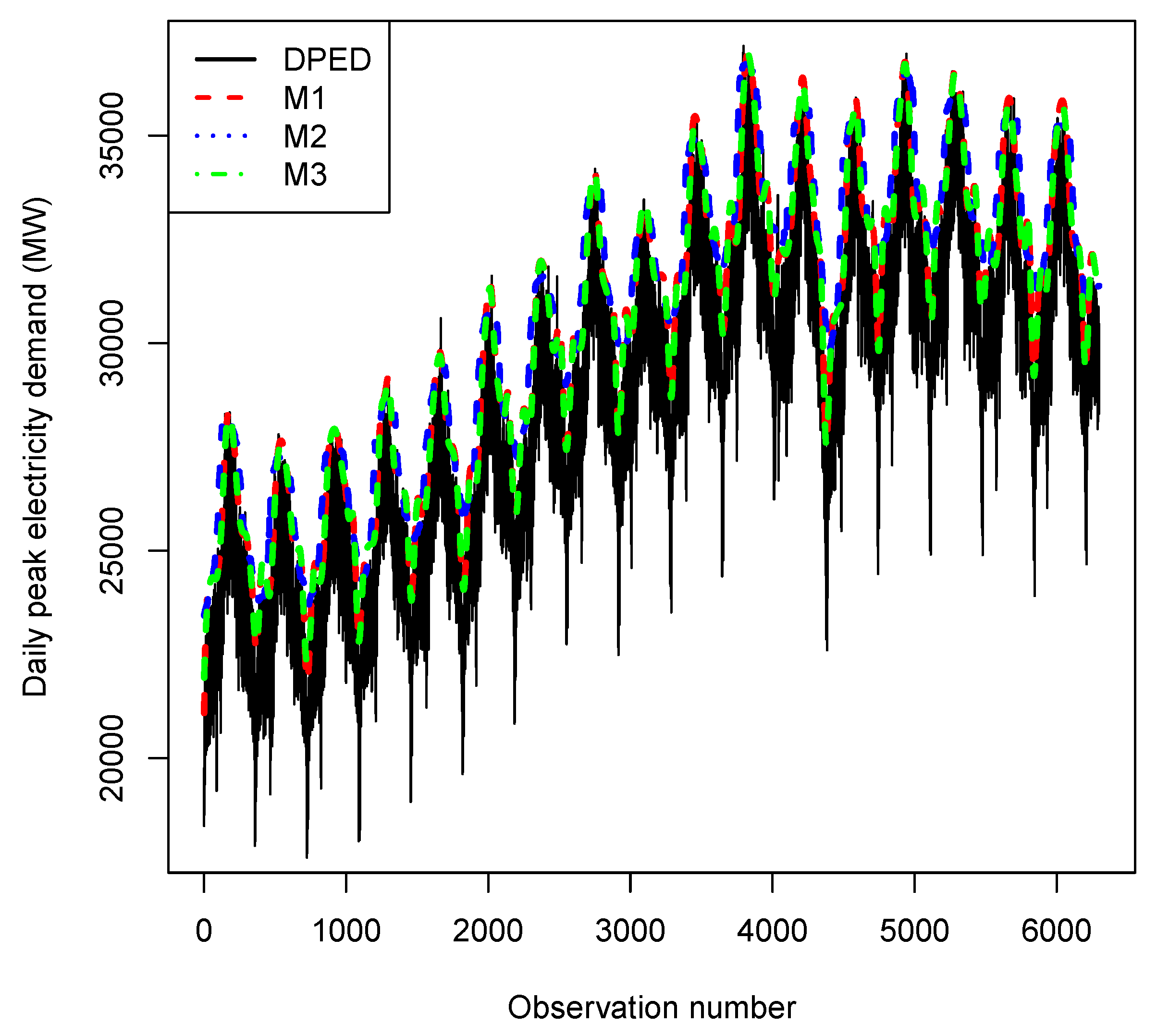
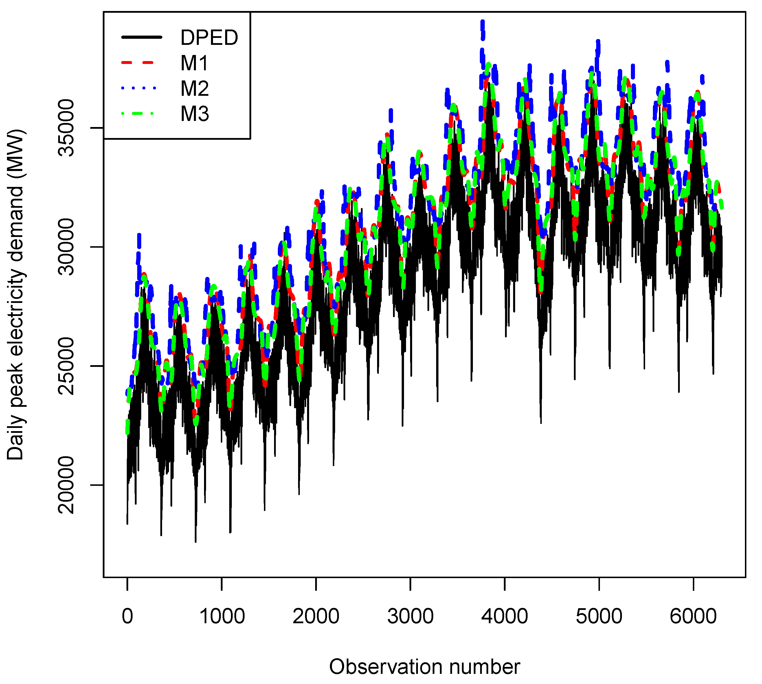
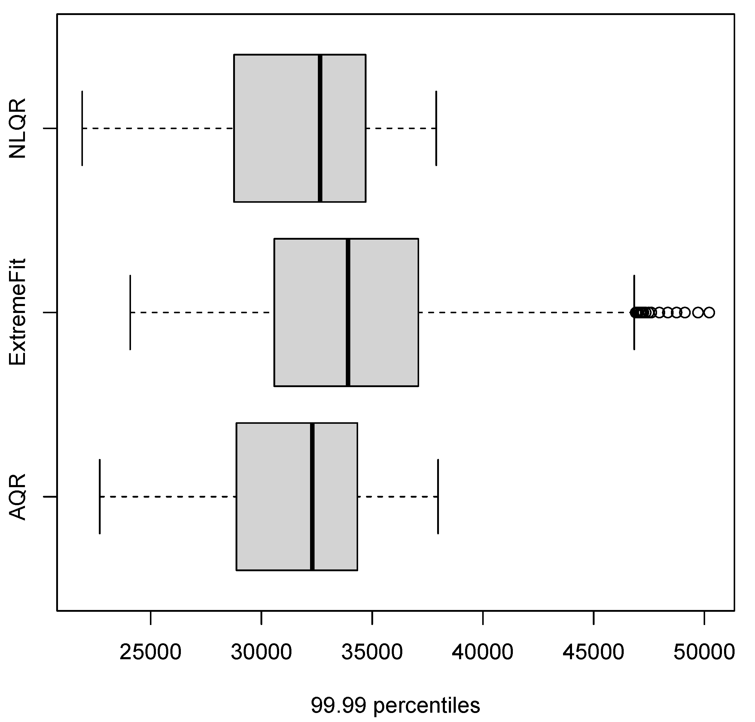
4. Empirical Results

4.1. Data and Software

The data used in this paper were from Eskom, South Africa’s power utility company. The data considered were Net Energy Sent Out (NESO). The NESO, measured in megawatts, is the rate at which electrical energy is delivered to customers. The NESO considered in this paper is the daily peak electricity demand (DPED), which is the maximum hourly demand in a 24 h period. Aggregated DPED data are used for the agricultural, commercial, domestic and industrial sectors of South Africa and were for the period January 1997 to May 2014, giving us a total of 6299 observations. The R statistical package Version 4.04 [48] was used in this study.

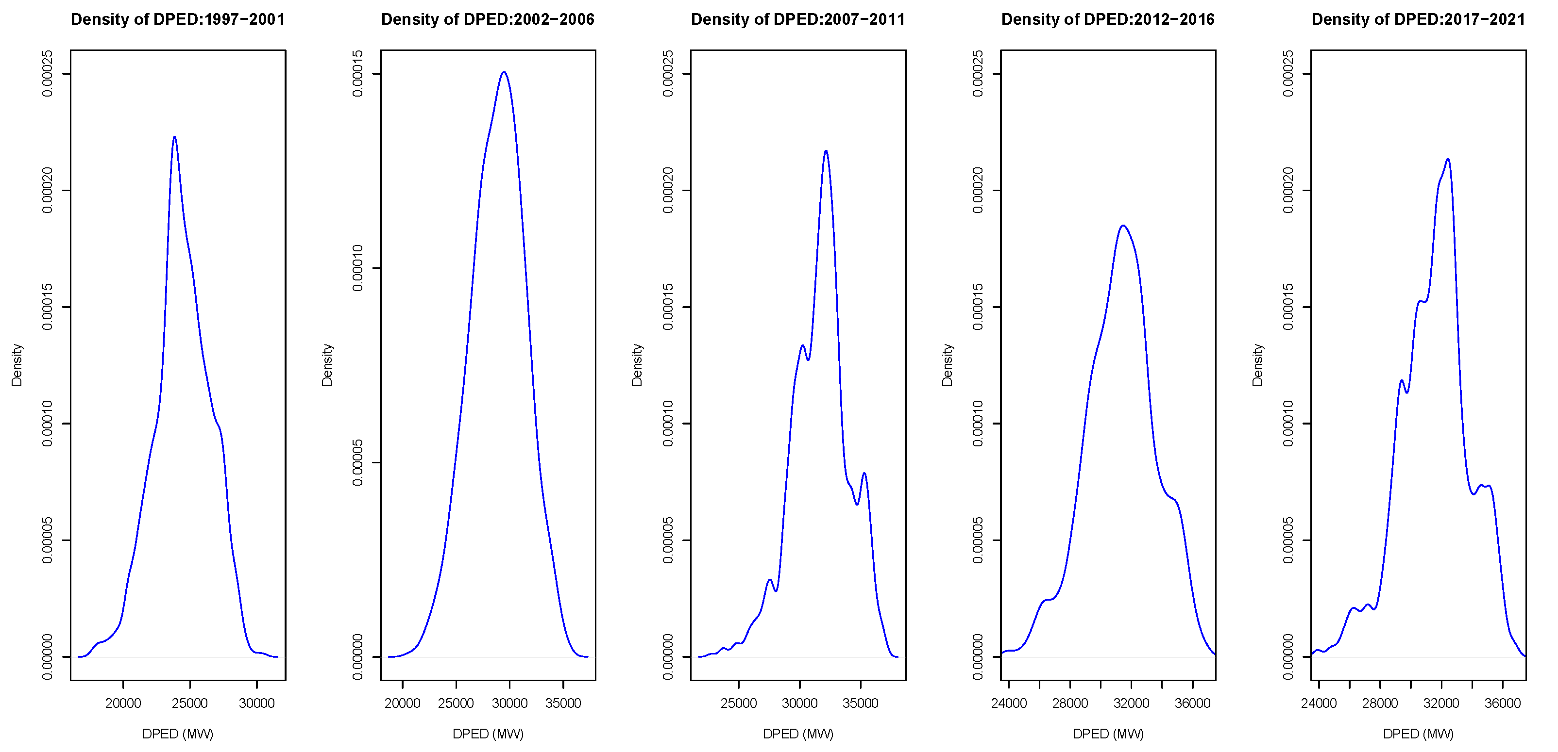
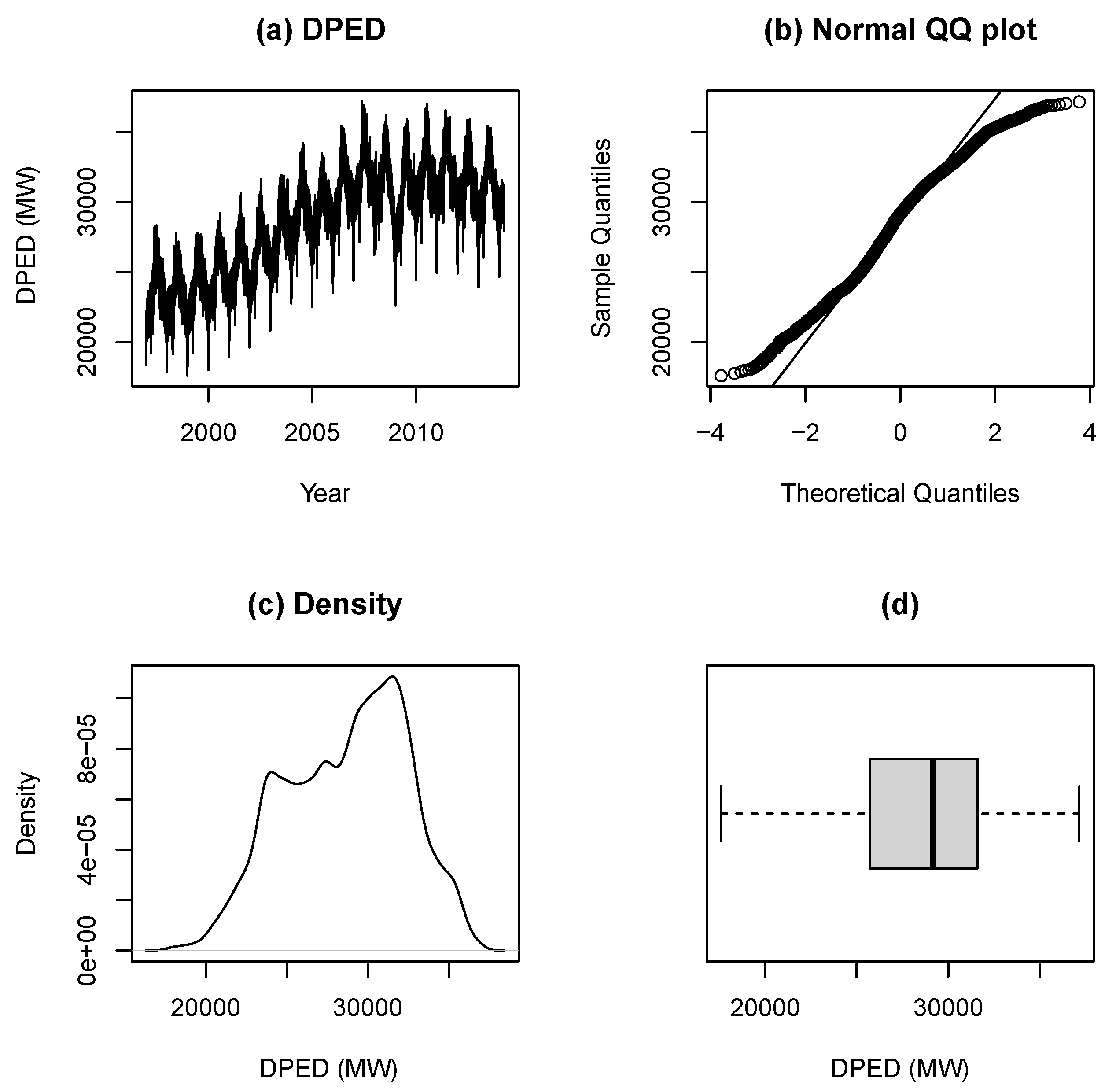
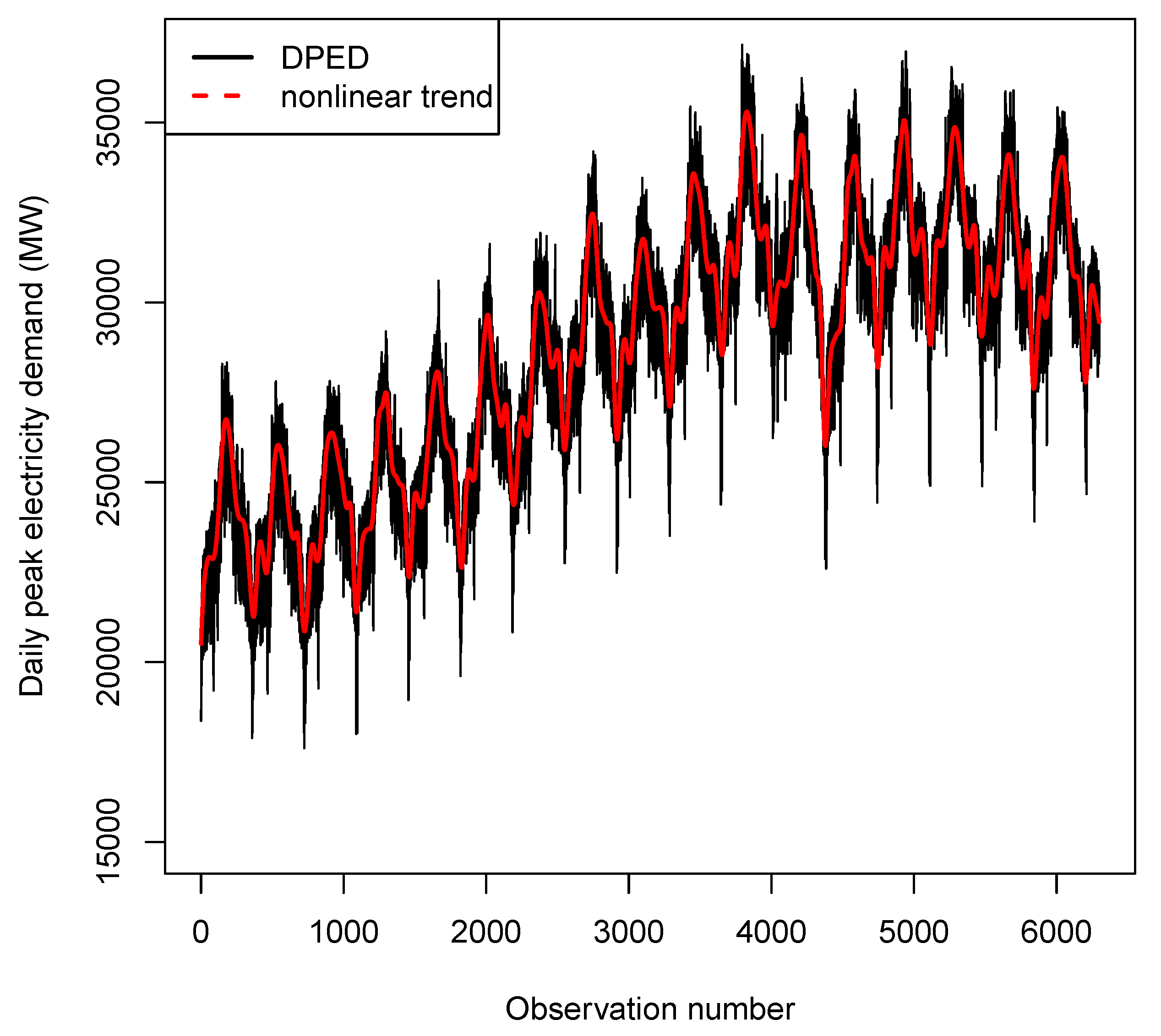
4.2. Exploratory Data Analysis
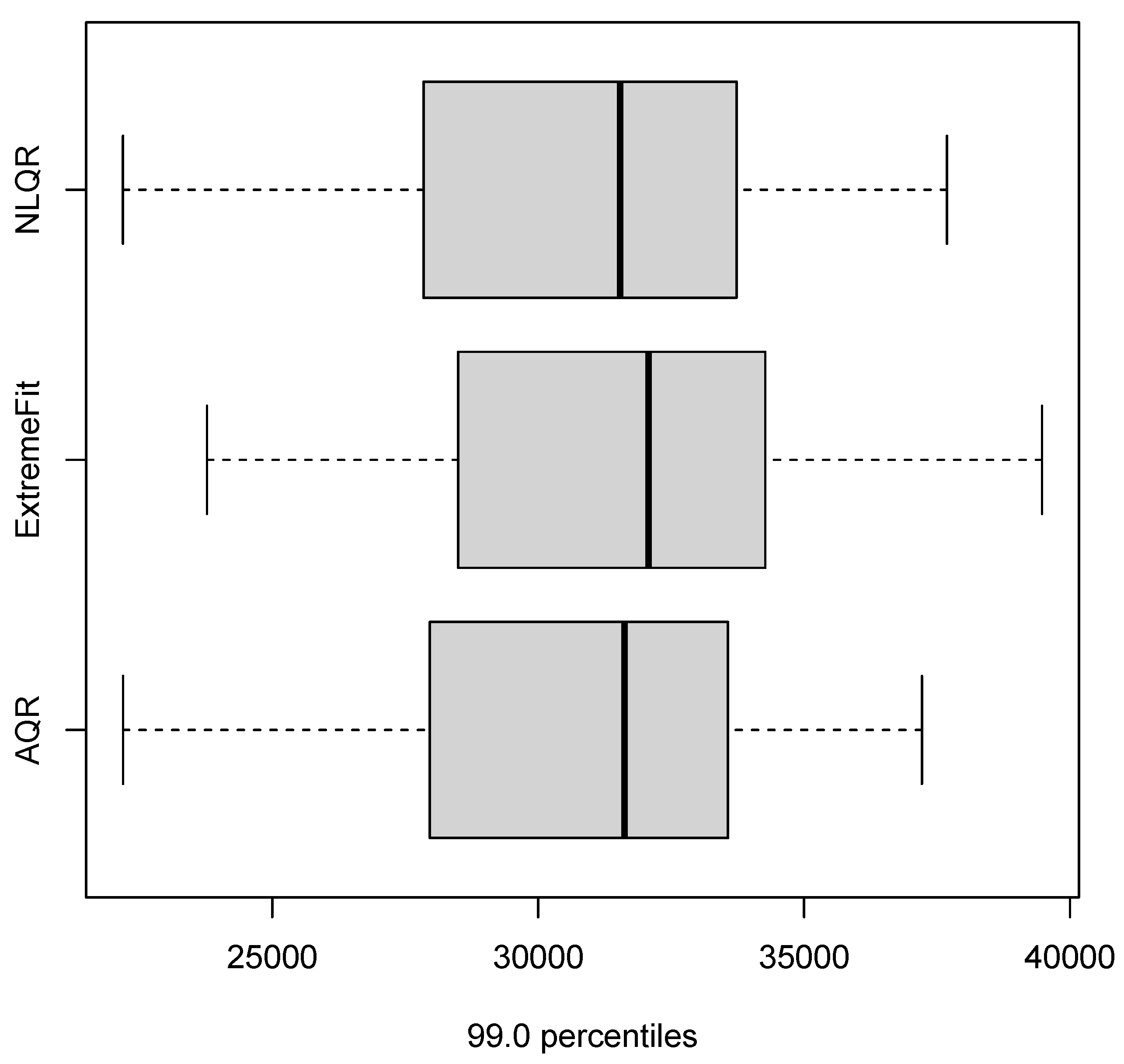
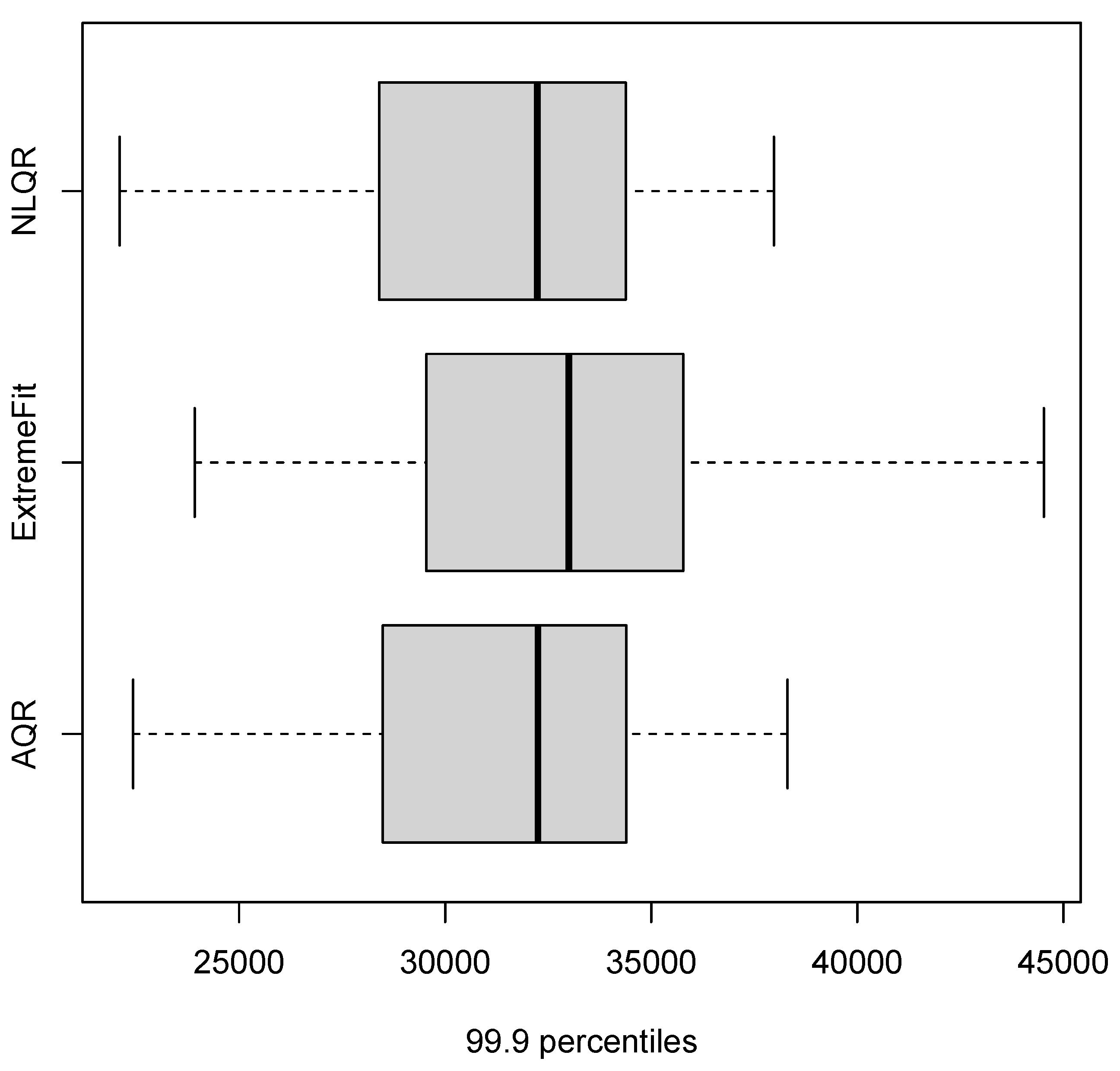
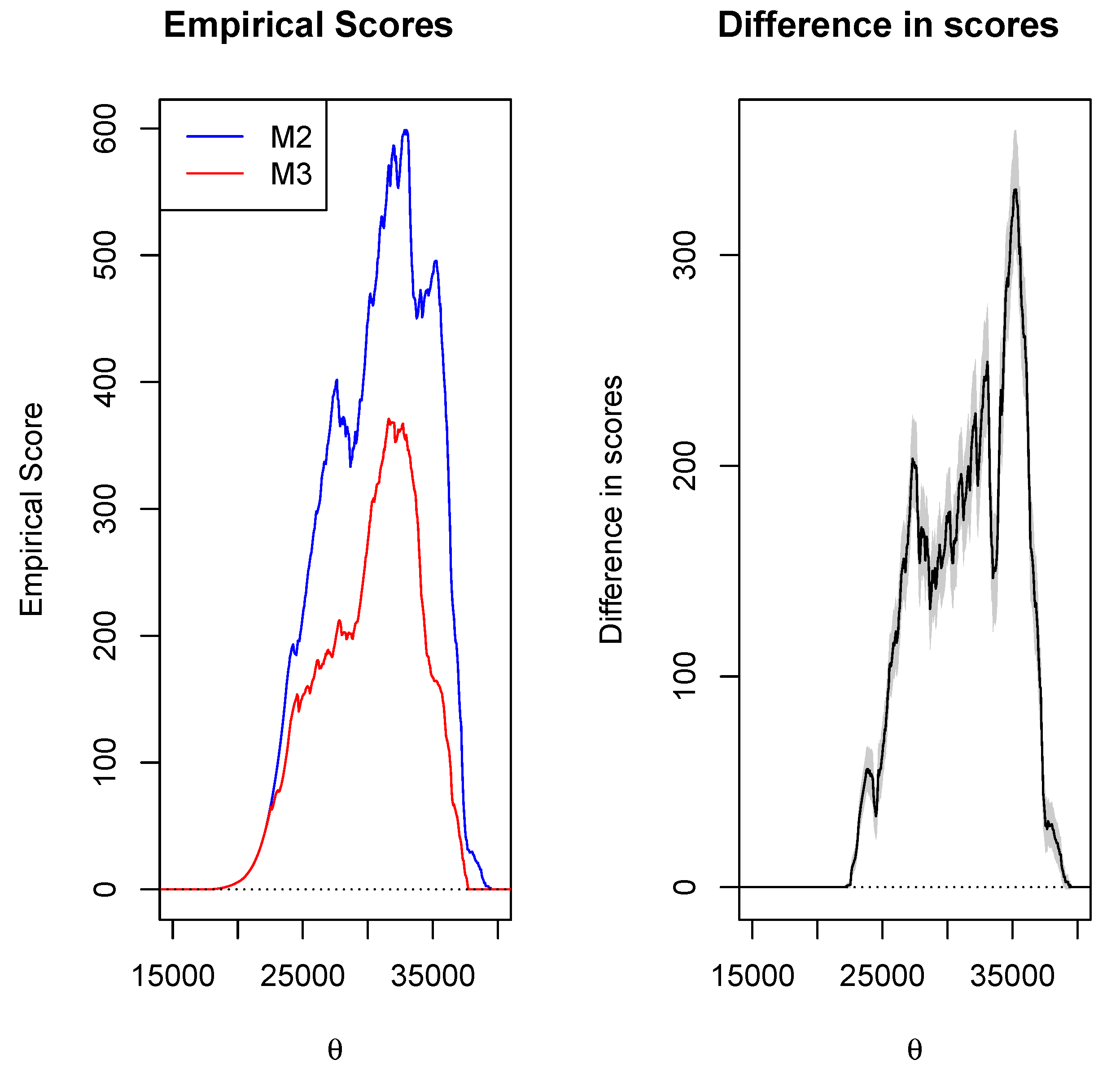
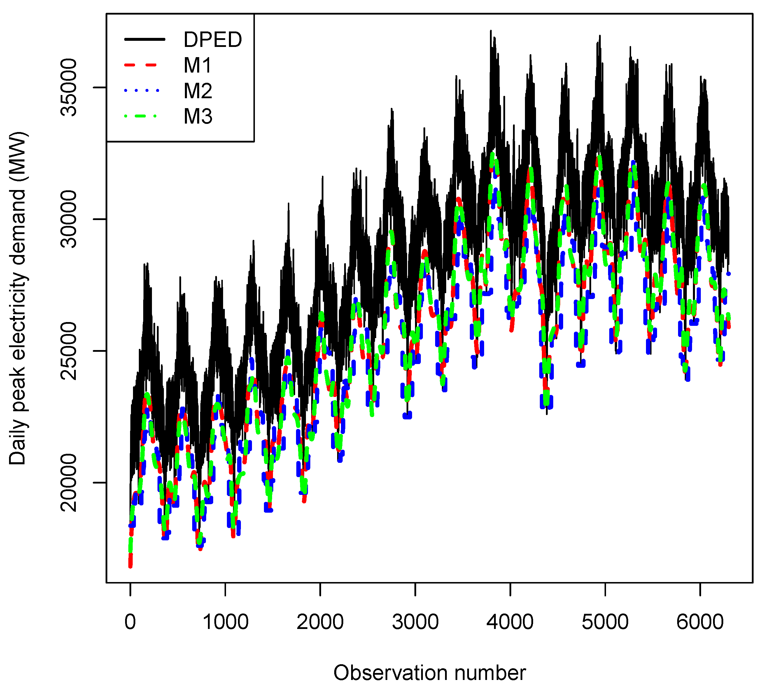
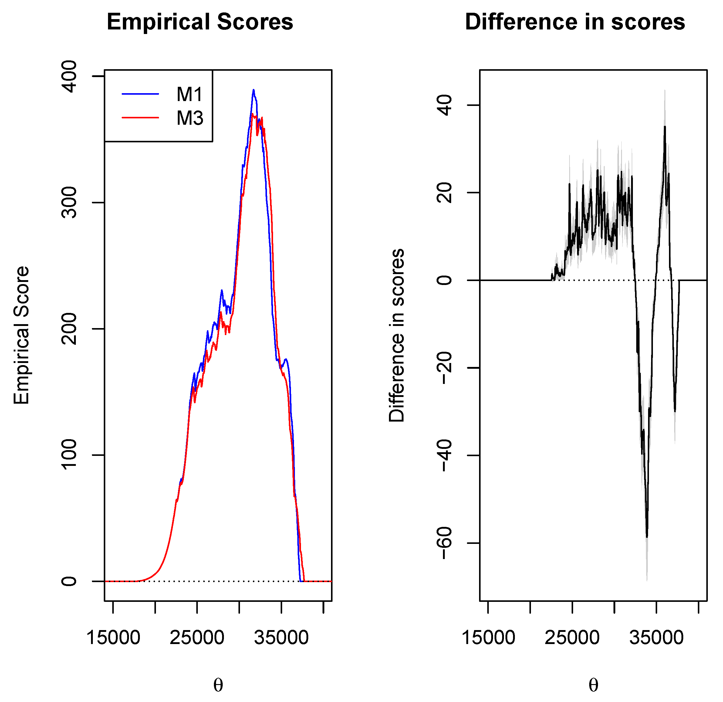
Table 3 presents the summary statistics of the DPED. The minimum and maximum DPED values during the sampling period were 17 605MW and 37 158MW, respectively. The skewness value was −0.232, showing that the distribution of the DPED was skewed to the left. The density (Panel (c)) and box (Panel (d)) plots given in Figure 1 confirm that the distribution of the DPED was negatively skewed.
Figure 1 (a) shows a plot of the DPED. The DPED data were not normally distributed as shown by Panel (b) of Figure 1.
A plot of the DPED superimposed with a nonlinear trend variable is given in Figure 2. A penalised cubic regression spline was used to obtain the nonlinear trend, which was used as a covariate for all the models, except for the extremal mixture model, where a linear trend was used as a covariate.
The penalised cubic regression smoothing spline model is given in Equation (19) as:
π ( t ) = i = 1 n y i f ( t i ) 2 + λ f ( t ) 2 d t ,
where y i denotes the DPED and λ is a smoothing parameter. The optimal estimate of the smoothing parameter λ was found based on the generalised cross-validation (GCV). Considering the AQR model, we have:
q Y | X ( τ ) = t = 1 n ρ τ y t , τ s τ ( noltrend ) , τ ( 0 , 1 ) .
In this study, we considered four quantile values, which were 0.95, 0.99, 0.999 and 0.9999, respectively.

4.3. Results

The probabilistic accuracy measures (scoring rules) were calculated as follows: we fit a parametric distribution to the forecasts and then estimated its parameters. The study considered a comparative analysis of three models, i.e., the AQR (M1), EM (M2) and NLQR (M3) models at 0.95, 0.99 and 0.9999 quantile forecasts. To evaluate the forecast accuracy measures of the AQR, EM and NLQR models, we used the CRPS, LogS, DSS, interval width and the pinball losses, as described in Section 3.5. We used the empirical scores of the CRPS, Logs, DSS, PL and interval width to evaluate the forecast performances. The lower the values of the scoring rules, the better the prediction performance was. The scoring rules were then computed based on the fitted parametric distribution.
A comparison of the models at both extremely high and extremely low quantiles is given in Table 4 and Table 5, respectively. At the 0.95 quantile, the EM model had the lowest CRPS, LogS and DSS, making it the best fitting model at this quantile level. The AQR model was the best fitting model at the 0.99, 0.999 and 0.9999 quantiles based on the CRPS and DSS evaluation metrics. Based on the prediction interval width coverage probability of 0.98 (see Table 4), all the models had valid coverage probabilities since they were all greater than 0.98. However, the EM model provided the largest coverage probability, which was 0.9886, and had the least number of observations below the 0.01 and 0.99 quantiles, respectively. As for the extremely low quantiles, the NLQR model had the smallest CRPS, LogS and DSS at the 0.05 quantile. At the 0.01 quantile, the AQR model had the smallest LogS and DSS values. The NLQR model was the best fitting model at the 0.001 quantile based on the CRPS, LogS and DSS evaluation metrics.
Figure 3, Figure 4 and Figure 5, respectively, show the DPED superimposed with the 0.95, 0.99 and 0.01 quantiles from the M1, M2 and M3 models, respectively. All figures reflect the peak identification in the electricity demand based on the 0.95, 0.99 and 0.999 quantiles of the DPED data. Furthermore, Figure 3, Figure 4 and Figure 5 show the black solid line depicting the DPED from January 1997 to May 2014, the red dotted line the M1 model distribution, the blue dotted line the M2 model and the green dotted line the M3 model distribution, respectively. Model M2 gave the best results at the 0.95 quantile.
Figure 6, Figure 7 and Figure 8, respectively, show three box plots of the 0.99, 0.999 and 0.9999 quantiles with the AQR, EM and NLQR models. The box plots for the EM model have shorter left tails and longer right tails compared to the other two models, AQR and NLQR, respectively. The medians of the AQR and NLQR models are all at the same level; however, their box plots show very different distributions for the DPED data.
Figure 9 shows the forecast distributions for the DPED data from 1997 to 2021. It also summarises the forecast distributions drawn at each specific date interval. For every five years, the histogram represents a sample from the model’s forecast distribution.
The Murphy diagrams in Figure 10, Figure 11 and Figure 12 show empirical scores and differences in scores for the M1 and M2, M1 and M3 and M2 and M3 models, respectively. A negative difference means that the regime-switching forecast is preferable. It must be noted that Murphy diagrams (Figure 10, Figure 11 and Figure 12) might lead to inconclusive situations in which neither of the three forecast methods dominates the other, and as a result, it would be unhelpful in decision-making. The p-values of the three models for three different forecasting horizons were analysed. Based on the information given in Section 3.4, the forecast accuracies of the 0.95, 0.99, 0.999 and 0.9999 quantiles are summarised. Since all p-values were less than 0.05, we, therefore, rejected the null hypothesis that there was no significant difference in the predictive abilities amongst the models. The forecasting performance of all the models was significant. Hence, the forecasting accuracy of M1 was better than that of the M2 and M3 models in extremely high quantiles, and the M3 model was better than the M1 and M2 models in extremely low quantiles.

5. Discussion

The current study was motivated by the need to accurately predict the largest possible demand for electricity at any given point in time. This can help system operators in shifting demand to off-peak periods including the scheduling of generating units during peak periods.
The study carried out a comparative analysis of the AQR, EM and NLQR models in predicting extremely high and extremely low quantiles of daily peak electricity demand. Other approaches, for example [4,13,32] among others, underestimated conditional quantiles or failed to estimate extreme conditional quantiles from their proposed models.
The additive quantile regression models are becoming increasingly popular in many applications as they are known to be flexible and robust. The AQR model does not require a predetermined function fit; however, it determines the best fit from the DPED data under extremely high quantiles. Table 4 shows the AQR model as a powerful method as suggested by the low evaluation metrics. Table 5 shows NLQR to be the best fitting model for extremely low quantiles.
The predictive performance of the models was evaluated based on three evaluation metrics, the CRPS, LogS and DS, respectively. The models were compared based on these scoring rules. The comparative forecast evaluation is generally applauded for giving critical features with out-of-sample forecasts in modelling comparison. The AQR model showed the smallest values of the scoring rules in all three extremely high quantiles, except for one quantile. All sets of scores’ (CRPS, LogS and DSS) values in Table 4 suggest that the M1 model was the best model, while Table 5 suggests that M3 was the best fitting model. Hence, the model M1 provided the highest predictive accuracy at the 0.95 and 0.99 quantiles, respectively, as given in both Figure 3 and Figure 4.
The accurate predictions in extreme conditional quantiles of electricity demand in this study are necessary for planning power systems and assessing investment projects in South Africa. Based on the Murphy diagrams, M1 (AQR model) had the highest predictive ability compared to the extremal mixture and nonlinear quantile regression models. The question of model comparisons in both extremely high and low quantiles in this study arises from the need to:
  • Address the uncertainties that seem to be ignored in practice (for example, the uncertainty in the process that is generating the occurrence of the extreme events);
  • Quantify the uncertainties in the estimated parameters of the distribution;
  • Predict extremely high quantiles of daily peak electricity demand. This helps system operators know the possible largest demand, which will enable them to supply adequate electricity to consumers and shift load to off-peak periods.
A limitation of this study is that the sample data were for the period 1997–2014. It would have been good to cover the period of the COVID-19 pandemic. However, at the time of the study, the data covering the pandemic period were not available to the researchers. This would have helped in seeing the impact of the pandemic on electricity demand. Future research, when data are made available, should include this period. Other future research directions would include the inclusion of more covariates such as meteorological and economic including calendar variables so that we may capture their effect on the prediction of extremely high and extremely low electricity demand.

6. Conclusions

The paper presented a comparative analysis of the prediction of extremely high and extremely low daily peak electricity demand. An extremal mixture model in which a kernel density was fit to the bulk model and a Pareto distribution fit to the tail model was compared with an additive quantile regression and a nonlinear quantile regression models. The results indicated that the additive quantile regression model produces the most accurate predictions at both extremely high and low quantile levels. Furthermore, the additive quantile regression and nonlinear quantile regression models fit well based on the Murphy diagrams for the comparison of the 0.99 quantile compared to the other models. The results from this study could be useful to decision-makers in power utility companies in the prediction of extremely high and low electricity demand, thereby assisting them in the management of the risk of overprediction and underprediction.

Author Contributions

Conceptualization, N.M. and C.S.; methodology, N.M., C.S. and E.R.; software, N.M. and C.S.; validation, N.M., C.S. and E.R.; formal analysis, N.M.; investigation, N.M.; data curation, N.M.; writing—original draft preparation, N.M.; writing—review and editing, N.M., C.S. and E.R.; visualization, N.M. and C.S.; supervision, C.S. and E.R.; project administration, C.S. and N.M. All authors read and agreed to the published version of the manuscript.

Funding

This research received no external funding.

Institutional Review Board Statement

Not applicable.

Informed Consent Statement

Not applicable.

Data Availability Statement

The data used in this study were provided by Eskom, South Africa’s power utility company.

Acknowledgments

The authors are grateful to Eskom, South Africa’s power utility company, for providing the data, the University of Limpopo, the University of Venda and the University of South Africa for their resources and numerous people for helpful comments on this paper.

Conflicts of Interest

The authors declare no conflict of interest.

Abbreviations

The following abbreviations are used in this manuscript:
AQRAdditive quantile regression
ARAutoregressive
CDFCumulative distribution function
CPCoverage probability
CRPSContinuous rank probability score
DPDDaily peak demand
DPEDDaily peak electricity demand
DSSDawid–Sebastiani score
EQRExtreme quantile regression
EVTExtreme value theory
GARCHGeneralized autoregressive conditional heteroskedasticity
GCVGeneralised cross-validation
GDPGross domestic product
GEVDGeneralised extreme value distribution
GJRGlosten–Jagannathan–Runkle
GLDGeneralised logistic distribution
GPDGeneralised Pareto distribution
GSPGeneralised single Pareto distribution
IWInterval width
L M d Lower median
LogSLogarithmic score
M d Median
MSREMean-squared relative error
NDPNational Development Plan
NPOTNonparametric peaks-over-threshold
PDFProbability density function
PLPinball loss
POTPeaks-over-threshold
QRQuantile regression
quantGAMQuantile generalised additive model
REIPPPPRenewable Energy Independent Power Producer Program
U M d Upper median
USBUnited States Bancorp

References

  1. Larmuth, J.; Cuellar, A. An updated review of South African CSP projects under the renewable energy independent power producer procurement programme (REIPPPP). In AIP Conference Proceedings; AIP Publishing LLC: Melville, NY, USA, 2019; Volume 2126, p. 040001. [Google Scholar]
  2. Stands, S.R. Utility-Scale Renewable Energy Job Creation: An Investigation of the South African Renewable Energy Independent Power Producer Procurement Programme (REIPPPP). Bachelor’s Thesis, Stellenbosch University, Stellenbosch, South Africa, 2015. [Google Scholar]
  3. Do, L.P.C. Using Quantile Regression for Modeling of Electricity Price and Demand. Master’s Thesis, NTNU, Trondheim, Norway, 2015. [Google Scholar]
  4. Beirlant, J.; Wet, T.D.; Goegebeur, Y. Nonparametric estimation of extreme conditional quantiles. J. Stat. Comput. Simul. 2004, 74, 567–580. [Google Scholar] [CrossRef]
  5. Gardes, L.; Girard, S.; Lekina, A. Functional nonparametric estimation of conditional extreme quantiles. J. Multivar. Anal. 2010, 101, 419–433. [Google Scholar] [CrossRef] [Green Version]
  6. Kukush, A.; Beirlant, J.; Goegebeur, Y. Nonparametric estimation of extreme conditional quantiles. In KU Leuven DTEW Research Report; Departement Toegepaste Economische Wetenschappen: Leuven, Belgium, 2005; p. 557. [Google Scholar]
  7. Wang, H.J.; Li, D. Estimation of extreme conditional quantiles through power transformation. J. Am. Stat. Assoc. 2013, 108, 1062–1074. [Google Scholar] [CrossRef]
  8. Ndao, P.; Diop, A.; Dupuy, J.F. Nonparametric estimation of the conditional extreme-value index with random covariates and censoring. J. Stat. Plan. Inference 2016, 168, 20–37. [Google Scholar] [CrossRef] [Green Version]
  9. Sigauke, C.; Verster, A.; Chikobvu, D. Extreme daily increases in peak electricity demand: Tail quantile estimation. Energy Policy 2013, 53, 90–96. [Google Scholar] [CrossRef]
  10. Diriba, T.A.; Debusho, L.K.; Botai, J. Modeling extreme daily temperature using generalized Pareto distribution at Port Elizabeth, South Africa. Annu. Proc. S. Afr. Stat. Assoc. Conf. 2015, 2015, 41–48. [Google Scholar]
  11. Sigauke, C.; Nemukula, M.M.; Maposa, D. Probabilistic hourly load forecasting using additive quantile regression models. Energies 2018, 11, 2208. [Google Scholar] [CrossRef] [Green Version]
  12. Mallor, F.; Omey, E. An introduction to statistical modelling of extreme values. Hub Res. Pap. 2009, 36, 5–31. [Google Scholar]
  13. Gajowniczek, K.; Zabkowski, T. Two-stage electricity demand modeling using machine learning algorithms. Energies 2017, 10, 1547. [Google Scholar] [CrossRef] [Green Version]
  14. Chernozhukov, V. Extremal quantile regression. Ann. Stat. 2005, 33, 806–839. [Google Scholar] [CrossRef] [Green Version]
  15. Lerch, S.; Thorarinsdottir, T.L.; Ravazzolo, F.; Gneiting, T. Forecaster’s dilemma: Extreme events and forecast evaluation. Stat. Sci. 2017, 32, 106–127. [Google Scholar] [CrossRef]
  16. Jordan, A.; Krüger, F.; Lerch, S. Evaluating probabilistic forecasts with scoringRules. arXiv 2017, arXiv:1709.04743. [Google Scholar] [CrossRef] [Green Version]
  17. Daouia, A.; Gardes, L.; Girard, S. On kernel smoothing for extremal quantile regression. Bernoulli 2013, 19, 2557–2589. [Google Scholar] [CrossRef]
  18. Durrieu, G.; Grama, I.; Pham, Q.K.; Tricot, J.M. Nonparametric adaptive estimation of conditional probabilities of rare events and extreme quantiles. Extremes 2018, 18, 437–478. [Google Scholar] [CrossRef]
  19. D’Haultfœuille, X.; Maurel, A.; Zhang, Y. Extremal quantile regressions for selection models and the black–white wage gap. J. Econom. 2018, 203, 129–142. [Google Scholar] [CrossRef] [Green Version]
  20. Smith, R.L. Extreme value analysis of environmental time series: An application to trend detection in ground-level ozone. Stat. Sci. 1989, 4, 367–377. [Google Scholar]
  21. Grama, I.; Spokoiny, V. Statistics of extremes by oracle estimation. Ann. Stat. 2008, 36, 1619–1648. [Google Scholar] [CrossRef]
  22. Nindhin, K.; Chandran, C. Importance of generalized logistic distribution in extreme value modeling. Appl. Math. 2013, 4, 560–573. [Google Scholar] [CrossRef] [Green Version]
  23. Sigauke, C. Modelling Electricity Demand in South Africa. Ph.D. Thesis, University of the Free State, Bloemfontein, South Africa, 2014. [Google Scholar]
  24. Lebotsa, M.E.; Sigauke, C.; Bere, A.; Fildes, R.; Boylan, J.E. Short term electricity demand forecasting using partially linear additive quantile regression with an application to the unit commitment problem. Appl. Energy 2018, 222, 104–118. [Google Scholar] [CrossRef] [Green Version]
  25. Čepin, M.; Demin, M.; Danilov, M.; Romanenko, I.; Afanasyev, V. Power System Reliability Importance Measures. In Proceedings of the 29th European Safety and Reliability Conference, Hannover, Germany, 22–26 September 2019; pp. 1633–1637. [Google Scholar]
  26. Sigauke, C.; Nemukula, M.M. Modelling extreme peak electricity demand during a heatwave period: A case study. Energy Systems 2020, 11, 139–161. [Google Scholar] [CrossRef]
  27. Norouzi, N.; de Rubens, G.Z.; Choubanpishehzafar, S.; Enevoldsen, P. When pandemics impact economies and climate change: Exploring the impacts of COVID-19 on oil and electricity demand in China. Energy Res. Soc. Sci. 2020, 68, 10165. [Google Scholar] [CrossRef] [PubMed]
  28. Lu, H.; Ma, X.; Ma, M. A hybrid multi-objective optimizer-based model for daily electricity demand prediction considering COVID-19. Energy 2021, 2019, 119568. [Google Scholar] [CrossRef] [PubMed]
  29. Liu, X.; Lin, Z. Impact of COVID-19 pandemic on electricity demand in the UK based on multivariate time series forecasting with bidirectional long short term memory. Energy 2021, 227, 120455. [Google Scholar] [CrossRef]
  30. Alasali, F.; Nusair, K.; Alhmoud, L.; Zarour, E. Impact of the COVID-19 Pandemic on Electricity Demand and Load Forecasting. Sustainability 2021, 13, 1435. [Google Scholar] [CrossRef]
  31. Muller, A.; Arnaud, P.; Lang, M.; Lavabre, J. Uncertainties of extreme rainfall quantiles estimated by a stochastic rainfall model and by a generalized Pareto distribution/Incertitudes des quantiles extrêmes de pluie estimés par un modèle stochastique d’averses et par une loi de Pareto généralisée. Hydrol. Sci. J. 2009, 54, 417–429. [Google Scholar] [CrossRef]
  32. Gardes, L.; Girard, S. Conditional extremes from heavy-tailed distributions: An application to the estimation of extreme rainfall return levels. Extremes 2010, 13, 177–204. [Google Scholar] [CrossRef] [Green Version]
  33. Cai, Y.; Reeve, D.E. Extreme value prediction via a quantile function model. Coast. Eng. 2013, 77, 91–98. [Google Scholar] [CrossRef] [Green Version]
  34. Chavez-Demoulin, V.; Embrechts, P.; Sardy, S. Extreme quantile tracking for financial time series. J. Econom. 2014, 181, 44–52. [Google Scholar] [CrossRef]
  35. Gijbels, I.; Karim, R.; Verhasselt, A. Semiparametric quantile regression using quantile-based asymmetric. Comput. Stat. Data Anal. 2020, 157. [Google Scholar] [CrossRef]
  36. Taylor, J.W. Evaluating quantile-bounded and expectile-bounded interval forecasts. Int. J. Forecast. 2021, 37, 800–811. [Google Scholar] [CrossRef]
  37. Durrieu, G.; Grama, I.; Jaunatre, K.; Pham, Q.K.; Tricot, J.M. Extremefit: A Package for Extreme Quantiles. J. Stat. Softw. 2018, 87, 1–20. [Google Scholar] [CrossRef] [Green Version]
  38. Wu, G.; Qiu, W. Threshold Selection for POT Framework in the Extreme Vehicle Loads Analysis Based on Multiple Criteria. Shock Vib. 2018. [Google Scholar] [CrossRef]
  39. Verster, A.; De Waal, D.; van der Merwe, S. Selecting an optimum threshold with the Kullback-Leibler deviance measure. JOSA A 2013, 30, 1687–1697. [Google Scholar]
  40. Gaillard, P.; Goude, Y.; Nedellec, R. Additive models and robust aggregation for GEFCom 2014 probabilistic electric load and electricity price forecasting. Int. J. Forecast. 2016, 32, 1038–1050. [Google Scholar] [CrossRef]
  41. Fasiolo, M.; Goude, Y.; Nedellec, R.; Wood, S.N. Fast calibrated additive quantile regression. J. Am. Stat. Assoc. 2020, 1–11. [Google Scholar] [CrossRef] [Green Version]
  42. Koenker, R. Quantile Regression; Cambridge University Press: New York, NY, USA, 2005. [Google Scholar]
  43. Koenker, R.; Park, B.J. An interior point algorithm for nonlinear quantile regression. J. Econom. 1996, 71, 265–283. [Google Scholar] [CrossRef] [Green Version]
  44. Manikandan, S. Measures of central tendency: Median and mode. J. Pharmacol. Pharmacother. 2011, 3, 214. [Google Scholar] [CrossRef] [PubMed] [Green Version]
  45. Wei, W. Calibration Tests to Evaluate Probabilistic Forecasts and Temporal Modelling to Monitor Infectious Diseases. Ph.D. Thesis, University of Zürich, Zürich, Switzerland, 2016. [Google Scholar]
  46. Gneiting, T.; Katzfuss, M. Probabilistic forecasting. Annu. Rev. Stat. Appl. 2014, 1, 125–151. [Google Scholar] [CrossRef]
  47. Hyndman, R.J. Quantile Forecasting with Ensembles and Combinations. 2020. Available online: https://robjhyndman.com/publications/quantile-ensembles/ (accessed on 11 January 2021).
  48. R Core Team. R: A Language and Environment for Statistical Computing. 2021. Available online: https://www.R-project.org/ (accessed on 22 January 2021).
Figure 1. DPED plot (a), Q-Q plot (b), density plot (c) and box plot (d).
Energies 14 06704 g001
Figure 2. Daily peak electricity demand superimposed with a nonlinear trend.
Energies 14 06704 g002
Figure 3. DPED superimposed with the 0.95 quantiles from the M1, M2 and M3 models.
Energies 14 06704 g003
Figure 4. DPED superimposed with the 0.99 quantiles from the M1, M2 and M3 models.
Energies 14 06704 g004
Figure 5. DPED superimposed with the 0.01 quantiles from the M1, M2 and M3 models.
Energies 14 06704 g005
Figure 6. Box plots of the 0.99 quantile.
Energies 14 06704 g006
Figure 7. Box plots of the 0.999 quantile.
Energies 14 06704 g007
Figure 8. Box plots of the 0.9999 quantile.
Energies 14 06704 g008
Figure 9. Distributions for the DPED for every five years.
Energies 14 06704 g009
Figure 10. Murphy diagrams for the comparison of the 0.99 quantiles of AQR99 and Extremal99 (M1 and M2).
Energies 14 06704 g010
Figure 11. Murphy diagrams for the comparison of the 0.99 quantiles of AQR99 and NLQR99 (M1 and M3).
Energies 14 06704 g011
Figure 12. Murphy diagrams for the comparison of the 0.99 quantiles of Extremal99 and NLQR99 (M2 and M3).
Energies 14 06704 g012
Table 1. Summary of previous studies on the modelling and estimation of extremely high quantiles.
AuthorsDataModelsMain Findings
Muller et al. [31]Marseilles hourly rainfall data from 1882–2003GPD and SHYPRE hourly rainfall stochastic models.Results show that both methods give similar results and have similar uncertainties. Moreover, the sensitivity of the GPD to the shape parameter is quite high.
Gardes and Girard [32]French hourly rainfall data from 1993–2000Nearest neighbour model.The results show that the nearest neighbour Hill estimator gives the same weight to all the largest observations.
Sigauke et al. [9]Eskom aggregated DPD data from 2000–2011GSP distribution and GPD models.The Q-Q plot of the GSP distribution incorporates most extreme observations in the tail slightly better than the GPD.
Cai and Reeve [33]Venice sea-level data from 1931–1981Semiparametric, QR, and parametric quantile function models.The performances of the parametric and the semiparametric approaches are very similar at the lower quantile levels. However, the performance of a quantile function modelling approach may vary from dataset to dataset at high quantile levels.
Chavez-Demoulin et al. [34]USB data from 27 June 2002 to 18 May 2010NPOT and classical POT models.The results of NPOT confirmed a rather precise and adapted estimation of high quantile-based risk measures for financial time series.
Diriba et al. [10]Port Elizabeth weather station data from 1949–2013GPD model.The GPD model for the minimum daily winter temperature shows no improvement in the parameter estimates’ precision.
Gijbels et al. [35]Hurricane data from 1971–2017Semiparametric and nonparametric models.The results show that the semiparametric model provides the smallest estimated prediction error compared to the nonparametric model.
Taylor [36]Hourly Nord Pool market prices data from 2013–2018AR-GJR-GARCH and AR models.The results show that the AR-GJR-GARCH model performs better than the AR model for both wider and narrower quantile intervals.
Table 2. Comparison of the models.
ModelsStrengthsWeaknesses
M1 (AQR)1. A hybrid model that combines GAMS with QR.
2. Estimation is distribution free.
3. Robust to outliers in the response variable.
1. Requires a smoothing function of the covariates.
2. Parameters are harder to estimate.
3. Does not give any details about the size of the high level of possible exceedances.
M2 (EM)1. Semiparametric extremal mixture model.
2. Based on one covariate, which is t = 1 , , n .
1. Has limitations on accuracy and stability.
2. Very sensitive to numbers and the location of the measured points.
M3 (NLQR)1. Inference is performed based on large sample approximation.
2. Robust to outliers in the response variable.
1. Requires a smoothing parameter.
2. Outliers only have an influence on quantile curves close to them, i.e., they affect extreme quantiles
Table 3. Descriptive statistics of DPED.
VarMinQ1MeanMedianQ3MaxSkewKurt
DPED17,60525,70628,68829,14931,59637,158−0.2322.287
Table 4. Model comparisons (extremely high quantiles).
95.0 th percentiles (0.95 quantile)
ModelsCRPSLogSDSSPL
M1 (AQR)2144.5469.608817.4418165.9795
M2 (EM)2069.7899.556017.3701209.2725
M3 (NLQR)2155.8759.611617.4495161.9122
M4 (Median)2155.8759.611617.4495165.5629
99.0 th percentiles (0.99 quantile)
ModelsCRPSLogSDSSPL
M1 (AQR)2125.4579.594717.425643.2765
M2 (EM)2131.232inf17.431556.8979
M3 (NLQR)2163.629inf17.459842.6107
M4 (Median)2163.629inf17459843.2509
99.9 th percentiles (0.999 quantile)
ModelsCRPSLogSDSSPL
M1 (AQR)2172.784inf17.47595.529
M2 (EM)2426.084inf17.75097.9267
M3 (NLQR)2190.201inf17.49585.3599
M4 (Median)2190.201inf17.49585.4869
99.99 th percentiles (0.9999 quantile)
ModelsCRPSLogSDSSPL
M1 (AQR)2168.997inf17.47470.6116
M2 (EM)2945.86inf18.38821.0272
M3 (NLQR)2202.221inf17.51490.6053
M4 (Median)2202.221inf17.51490.6274
Interval widths for the 0.01 and 0.99 quantiles (CP = 0.98)
ModelsAve IWCov ProbBelow 0.01 quantileAbove the 0.99 quantile
M1 (AQR)53640.98335946
M2 (EM)68070.98865220
M3 (NLQR)53120.98066557
M4 (Median)53850.98435643
Table 5. Model comparisons (extremely low quantiles).
5.0 th percentiles (0.05 quantile)
ModelsCRPSLogSDSSPL
M1 (AQR)3826.12510.396219.1919226.0744
M2 (EM)4225.65110.563519.6090287.7971
M3 (NLQR)3789.17410.380419.1481220.9624
M4 (Median)3789.17410.380419.1481224.6259
1.0 th percentiles (0.01 quantile)
ModelsCRPSLogSDSSPL
M1 (AQR)4529.20610.689920.009864.0034
M2 (EM)5089.07310.930220.690379.2499
M3 (NLQR)4523.98410.690520.026463.6298
M4 (Median)4523.98410.690520.026464.45815
0.1 th percentiles (0.001 quantile)
ModelsCRPSLogSDSSPL
M1 (AQR)5050.38610.908620.62127.793396
M2 (EM)5257.61411.002220.90558.342102
M3 (NLQR)5033.64410.903720.61127.756549
M4 (Median)5033.64410.903720.61127.781235
Publisher’s Note: MDPI stays neutral with regard to jurisdictional claims in published maps and institutional affiliations.

