Fault Diagnosis of DCV and Heating Systems Based on Causal Relation in Fuzzy Bayesian Belief Networks Using Relation Direction Probabilities

Abstract

The state-of-the-art provides data-driven and knowledge-driven diagnostic methods. Each category has its strengths and shortcomings. The knowledge-driven methods rely mainly on expert knowledge and resemble the diagnostic thinking of domain experts with a high capacity in the reasoning of uncertainties, diagnostics of different fault severities, and understandability. However, these methods involve higher and more time-consuming effort; they require a deep understanding of the causal relationships between faults and symptoms; and there is still a lack of automatic approaches to improving the efficiency. The data-driven methods rely on similarities and patterns, and they are very sensitive to changes of patterns and have more accuracy than the knowledge-driven methods, but they require massive data for training, cannot inform about the reason behind the result, and represent black boxes with low understandability. The research problem is thus the combination of knowledge-driven and data-driven diagnosis in DCV and heating systems, to benefit from both categories. The diagnostic method presented in this paper involves less effort for experts without requiring deep understanding of the causal relationships between faults and symptoms compared to existing knowledge-driven methods, while offering high understandability and high accuracy. The fault diagnosis uses a data-driven classifier in combination with knowledge-driven inference with both fuzzy logic and a Bayesian Belief Network (BBN). In offline mode, for each fault class, a Relation-Direction Probability (RDP) table is computed and stored in a fault library. In online mode, we determine the similarities between the actual RDP and the offline precomputed RDPs. The combination of BBN and fuzzy logic in our introduced method analyzes the dependencies of the signals using Mutual Information (MI) theory. The results show the performance of the combined classifier is comparable to the data-driven method while maintaining the strengths of the knowledge-driven methods.

1. Introduction

Recent advances in Information and Communications Technology (ICT), especially in embedded systems, enable the development of embedded control systems that profoundly couple our physical world to the computation world. Demand Controlled Ventilation (DCV) and heating systems, as a type of Heating, Ventilation, and Air Conditioning (HVAC) system, include many variables, signals, look-up tables, and components, with continuous and discrete dynamics. The complexity of a DCV and heating system increases when it becomes more extensive with more components and equipment that cooperate simultaneously. The complexity of HVAC systems makes them error-prone and susceptible to faults that may lead to a waste of energy, for example, continuous heating in the case of a stuck-at damper, poor thermal comfort, and unacceptable indoor air quality. Therefore, the occurrence of faults is unavoidable, and faults, for example, stuck-at or constant faults, inevitably occur. Despite the inherent complexity of DCV and heating systems, their applications require them to be fault and failure-tolerant. A fault- and failure-tolerant design of DCV and heating systems requires developments in failure detection and fault diagnosis techniques, which is a challenge. Detection and diagnostic techniques’ testing and evaluation activities are thus of critical importance for the early detection of faults in the models in the design phase before they propagate to the actual system. The failure detection and fault diagnosis in early stages of occurrence avoid threatening situations, the degradation of system performance, energy loss, or discomfort conditions [1]. For instance, the faults can be the reason for energy waste in HVAC systems up to 20% of total energy consumed, excess pollutant emissions, and decremented comfort for occupants [2,3]. Basarkar et al. describe how faults based on type and severity can be the reason for up to 22% of the total energy consumption of HVAC systems [4]. In HVAC systems, probable faults in building systems are various. For example, ASHRAE Project 1043-RP shows that a typical water-cooled centrifugal chiller can face more than twenty types of common faults [5]. ASHRAE Project 1312-RP indicated 68 types of common faults for a typical air handling unit [6]. Therefore, it is costly to capture sufficient training data for every fault, and most of the research projects consider only a part of these faults in most data-driven-based chiller FDD methods.

Many fault diagnosis methods have been reviewed and classified widely in many studies, for example, Steinder et al. [7] have focused explicitly on fault localization techniques in complex communication systems to find the exact source of a failure from a set of failure indications. They have classified the fault localization techniques into three categories of Artificial Intelligence (AI) techniques, that is, rule-based, model-based, and case-based systems, model traversing techniques, and fault propagation models, that is, code-based techniques, dependency graphs, Bayesian Networks (BNs), causality graphs, and phrase structured grammars.

Techniques for Fault Detection and Diagnosis (FDD) in the building energy system field can be categorized into knowledge-driven and data-driven methods [8]. Knowledge-driven methods resemble the diagnostic thinking of domain experts with a high capacity in reasoning of uncertainties; they can work with different fault severities. In contrast, methods in the data-driven category mainly rely on similarities and patterns [8]. Each category has its strengths and shortcomings. Zhao et al. studied 135 AI-based FDD papers from 1998 to 2018 and concluded that new AI-based methods are in demand that can combine the advantages of knowledge-driven and data-driven methods in the future [8]. The knowledge-driven methods rely mainly on expert knowledge and resemble the diagnostic thinking of domain experts with a high capacity in reasoning of uncertainties, they diagnose different fault severities, and are more understandable. On the other hand, these methods involve higher and more time-consuming effort, they require a deep understanding of the causal relationships between faults and symptoms, and there is still a lack of automatic approaches to improve the efficiency. The data-driven methods rely on similarities and patterns and they are very sensitive to changes of patterns and have more accuracy than the other knowledge-driven based methods, but they require massive data for training, cannot inform about the reason behind the result, and they represent black boxes with low understandability.

The research problem is thus the combination of knowledge-driven and data-driven diagnosis in DCV and heating systems to benefit from both categories. The diagnostic method presented in this paper involves less effort for experts and quicker approaches without requiring a deep understanding of the causal relationships between faults and symptoms compared to existing knowledge-driven methods while offering higher understandability than other data-driven approaches and higher accuracy than other knowledge-driven approaches resolved by data-driven-based category. The fault diagnosis uses a data-driven classifier in combination with knowledge-driven inference with both fuzzy logic and a Bayesian Belief Network (BBN). The combination of BBN and fuzzy logic in our introduced method analyzes the dependencies of the signals using Mutual Information (MI) theory.

In the offline mode, a library of trends and statuses based on training fault cases is established. The conditional probabilities are calculated based on fuzzy weights of signal values and statuses that are used to obtain mutual information. The positive MI values show the dependencies of the subdomains in a pair of measurement signals or statuses for each fault case (pairwise dependency) and negative MI values show that there is no dependency. Then, the conditional probabilities of the subdomains in a pair with positive MI values are calculated and the conditional probability with the higher value indicates the direction of the dependency in each pair of nodes. Then, these dependencies are stored in the offline library as the RDPs. In the online diagnosis mode, our strategy compares the trends and statuses of the real scenario, which can be a fault scenario, with the trends and statuses that are stored in the offline library to find the most similar trends and statuses of signals of the fault case to the trends and statuses of signals for example scenarios in the library. For this comparison, the RDP of the real or faulty scenario is compared to the RDPs in the offline library and the percentages of similarities are calculated. Then, the evaluation step determines and sorts the likely faults based on the comparison results from the highest degree of similarity to the lowest as the diagnostic classifier result. These percentages of similarities are beliefs sorted from the highest value to the lowest value where larger values imply a higher probability of the corresponding fault. The overall benefits are more understandability, less effort for experts, and higher diagnostic accuracy. Our strategy only needs expert knowledge to define fuzzy sets and the whole process can intelligently classify the faults compared to the other knowledge-based strategies. The evaluation results show that our strategy can accurately map a fault case to the predefined fault in the library.

The method is tested on a demand-controlled ventilation and heating system. Stuck-at or constant faults at temperature sensors, CO₂ sensors, heater actuators, and damper actuators were investigated. The evaluation results show that 97.22% of faults were truly diagnosed with better precision, F-score and accuracy compared to a deep neural network. The diagnosis method sorts the results based on the probability values, for example, the top ranks are the most likely diagnosis result. However, the method indicates that the average values of the performance metrics increase when considering more cumulative ranks, for example, top five ranks, instead of only the first rank.

Literature Review

Luo et al. have proposed a similar method for Sensory Fault Detection and Diagnosis (SFDD) [9]. In this paper, they have used a k-means data clustering algorithm and classified each new dataset into different clusters in which the dataset in the same cluster has high similarity. The featuring Centroid Score (CS) is used to detect this similarity, and the k-means algorithm detects the closest centroid by calculating the Euclidean distance between each dataset and its corresponding cluster CS. Through this clustering-based method, the fault-free sensor readings were close to the cluster’s centroids while those faulty ones would be far away. The proposed SFDD strategy consisted of database building for sensor fault detection, database building for sensor fault diagnosis, and online SFDD for measurement data. However, our approach uses MI and RDP tables to detect the closest fault to the new datasets. Besides, our approach is implemented not only for the sensor faults but also for actuators.

The BBN is one of the important approaches in fault diagnosis methods based on probabilistic theory for modeling uncertain knowledge and reasoning based on conditions of uncertainty, probabilities, and graph theory [10]. BBNs were introduced by J. Pearl in the 1980s [11]. BBNs can be combined with other approaches such as machine learning techniques, signed directed graphs, probabilistic ensemble learning, fuzzy theory, fault trees, and genetic algorithms. Qiu et al. explain that BBNs have effectively modeled probabilistic relationships in diagnostic situations by providing a framework for identifying critical probabilistic mappings [12]. Their Probabilistic method can link symptoms to failures by calculation of prior probabilities of faults. They defined the symptoms based on pure expert knowledge, for example, repair data log and consulting with experts in printers [12]. However, they have not implemented any data-driven method and used a single BBN for the FDD process, but our approach creates unique BBN for each RDP dataset. Their method also needs historical data and a system log for constructing the BBN.

Embedded control systems interact with the environment, and the sensory data and signals are measured continuously. Therefore, defining an appropriate conditional likelihood density function in BBNs for continuous attributes is critical. Tang et al. [10] have presented a Fuzzy Bayesian Network (FBN) for machinery fault diagnosis demanding intensive experience and expert knowledge described by the natural language, such as large, high, or fast. They used fuzzy logic to define the fuzzy events, mapped the system to those uncertain ones, and then produced the BBN. However, they have used a single BBN for the fault detection process, but our approach creates unique BBNs for each output RDP dataset. Their approach is also limited to expert knowledge.

In machine learning techniques from the data-driven-based methods, Hu et al. [13] have proposed an intelligent fault diagnosis network for refrigerant charge faults of a variable-refrigerant-flow air-conditioning system. This network is developed under the BBN theory. However, this method as a data-driven-based fault diagnosis is very costly to obtain sufficient training data for every fault [8].

In signed directed graphs, Peng et al. [14] have proposed a Multi-logic Probabilistic Signed Directed Graph (MPSDG) fault diagnosis approach in chemical processes based on the Bayesian inference. They show that the signed-directed graphs cannot be applied for complicated logic relations, but the authors have shown that the BNs can solve this complexity. They have two offline modeling and online diagnosis phases. In the offline mode, they have analyzed the historical data and deviation values and evaluated the priori probabilities of reason nodes and directed edges. However, constructing the SDG or MPSDG in systems with no historical data is not possible.

On the other hand, the Fuzzy Bayesian Belief Network (FBBN) combines the BBNs with the fuzzy theory. Chiu et al. proposed a fuzzy Bayesian classifier with case-based reasoning to improve diagnosis problems [15]. In this study, they have used fuzzy theory to define conditional density functions in BBNs to cope with the problem caused by continuous attributes. The accuracy and efficiency of this approach for decision-making applications have been proved by many studies [16]. The FBBN is often used as an effective method of uncertain knowledge representation and reasoning. Fuzzy sets are mathematical sets, the elements of which have degrees of membership derived from the concept of fuzzy logic, which was introduced by Lotfi A. Zadeh and Dieter Klaua in 1965 [17,18]. Several examples show the effectiveness of FBBNs in solving uncertain problems, applying Fuzzy sets, and calculating the probabilities of BBNs [19]. Yao et al. [19] have modeled a Fuzzy Dynamic Bayesian Network (FDBN) for fault diagnosis and reliability prediction in complex systems using various test information. The quantitative analysis of an FDBN can proceed along with forwarding (or predictive) analysis and backward (or diagnostic) analysis. They have presented a model in a fault diagnosis model with uncertain and dynamic information. Their work introduces a dynamic process to the BN to model a dynamic system. It includes modeling the BN, the fuzzy theory applied to BN, and Static BN (SBN) that can be converted to Dynamic Bayesian Network (DBN) models by introducing time dependency. They have used fuzzy theory to evaluate the system’s reliability with different language variables very high, high, medium-high, medium, intermediate low, low, and very low. However, they generated the BN based on the fault statistics and the fuzzy failure probabilities of root nodes, but in our approach, the starting point is the observations of the system attributes.

Intan et al. [20] have applied an FBBN for analyzing medial tracks. This paper has extended the MI concept using fuzzy theory to construct an FBBN based on learning BN structures using an information-theoretic approach introduced by Cheng et al. [21]. They used fuzzy labels to determine the relation between two fuzzy nodes. For example, they have found the relationship of the different disease labels with other factors in a record of data for different patients, for example, age, degree, and other types of diseases. However, they have used this method for analyzing a medical dataset for different patients and diseases; therefore, the application is different. Further, their approach only measured the causal relations in FBBN using the relation direction probabilities between different pairs of parents and children. However, in our approach, we used the causal relationships in FBBNs based on relation direction probabilities for fault diagnosis, and our approach includes two modes, an offline training mode, and an online diagnosis phase, to classify the fault cases.

A suitable Failure Detection and Fault Diagnosis (FDFD) system ensures the HVAC systems’ proper operation as these systems are subject to various errors, which can lead to malfunctions. HVAC systems fail typically when the actuators “stick” and no longer change their set point, despite the commands. This actuator failure can arise in several parts. For instance, a valve may stick at fully-open, fully-closed, or any intermediate setpoints. If an actuator sticks in an open or closed position for a specific period, some concerns are expected, for example, the energy waste or uncomfortable environment [22]. The pure knowledge-based diagnosis models are also developed, for example, a real-time black-box tool for a VAV AHU was developed by Shiazoki and Miyasaka using a signed directed graph. The signed directed graph model is a minimized rules-based model to lower the effort that can detect the symptoms of the faults to find the root cause [23]. However, the performance of the method depended on the thresholds set. The wrong thresholds setting can cause incorrect diagnosis. Threshold settings are also laborious and time-consuming. Shi et al. introduced a model using probabilistic representations for dependencies of faults and symptoms in a VAV AHU. The fault diagnostic model is developed based on a DBN to diagnose persistent and transient faults while maintaining the FDD system’s good performance [24]. However, calculation of the conditional probability values between the faults and symptoms is yet manual and depends on expert knowledge. In addition, for large systems, the amount of data might be unbearable. Therefore, many complicated faults may not be evaluated unless advanced modeling or sensing methods are used.

Zhao et al. [25] have proposed a three-layer Diagnostic BN (DBN) for chiller faults diagnosis based on the BBNs using a graphical and qualitative illustration of the intrinsic causal relationships among three layers of causal factors, faults, and fault symptoms, and this DBN can be constructed based on the probability analysis and graph theory. The prior probabilities of root nodes and prior probabilities of faults are the normalized frequencies of faults, and conditional probabilities show the relations of the nodes in three layers. With observed pieces of evidence, posterior probabilities for fault diagnosis can be calculated. This framework uses all beneficial information of the chiller concerned and chiller experts’ knowledge, the quantitative and qualitative knowledge from diverse sources is merged and has a strong ability to deal with incomplete or even conflicting information. However, there are major differences to our proposed method. They calculated the conditional probabilities using statistical or machine learning algorithms, while we have calculated them based on fuzzy weights. Further, our approach is constructed based on mutual information theory and the dependencies of the system attributes (i.e., signals) for each fault case using BBN theory, which only needs expert knowledge to define fuzzy sets. Zhao et al.’s mentioned approach is also highly dependent on expert knowledge, especially in calculating prior probabilities. In addition, they have defined rules to conclude the posterior probabilities, but we used the sorting technique showing that the top ranks show reasonable results with high accuracy.

Xiao et al. [26] presented a Diagnostic Bayesian Network (DBN) for Fault Detection and Diagnosis (FDD) of Variable Air Volume (VAV) terminals. In this method, the parameters of the DBN describe the probabilistic dependencies between faults and evidence. The inputs of the DBN are the evidence that can be obtained from the measurements in Building Management Systems (BMSs) and manual tests. The outputs are the probabilities of faults concerned. The structure of the DBN is a graphical illustration of experts’ diagnostic thinking, which can illustrate the relationships among faults and symptoms qualitatively. They have defined a table including the fault nodes, states of the system, rules for defining the states, and prior probabilities for each state. In this method, after determining the nodes, the state of each node should be defined. A fault node may have several states that help in estimating the conditional probabilities of the fault evidence given the fault. The rules in the defined table can determine the corresponding states. There are also specific tables and rules to define evidence nodes. The whole structure of this DBN depends on expert knowledge and the rules to define the system states. In another paper from these authors, Zhao et al. [27] have also developed a second study on diagnostic Bayesian networks (DBNs) for diagnosing faults in air handling units (AHUs) in buildings. This paper developed four DBNs to diagnose heating/cooling coils faults, sensors, and faults in a secondary chilled water/heating water supply. However, establishing the FDD strategy and BBN nodes is highly dependent on expert rules.

Cai et al. [28] have used two BNs for multiple-simultaneous faults with a multi-source information fusion-based fault diagnosis methodology. These BNs are established based on sensor data and observed information. The Bayesian network structure is established according to the cause-and-effect sequence of faults and symptoms. One BN is made based on sensor data, and the other is based on sensor data and observed information; however, the relationship between faults and symptoms is based on expert reasoning and purely knowledge-based.

The features are essential for fault diagnosis. Wang et al. [29] introduced a feature selection (FS) method that is proposed in their study for chiller Fault Diagnosis (FD) and merged the Bayesian network with distance rejection (DR-BN) to remove extra features. First, the candidate existing features that can be retained are nominated through the following criteria: high existent frequency of sensors installed on the field chillers, high sensitivity to faults, and small calculation. Supplemental features are added to achieve a better performance. However, in our introduced method, we have used a different technique for feature development: RDP generations in the fault library of offline mode and online diagnostic mode as features for each fault case.

Table 1 indicates an overview of the related works. In summary, the novelties and main contributions of this paper are based on the following points:

Table 1. Overview of the related works.

Related Works	Application Domain	FDD Method	Approach (e.g., Fuzzy Logic, BBN, Clustering, NN, Classification, …)	Data Collection, e.g., (Simulation/Historical Data)	Diagnostic Method		Assessment (e.g., Accuracy, Understandability, and Effort)
					Knowledge-Driven Method (Yes/No)	Data-Driven Method (Yes/No)
Luo et al. [9]	SFDD for chilled water system	Yes	Clustering-based SFDD & Data-Base Gathering Based on Centroid Score (CS)	Real sample information data	No	Yes	Low Expert Effort Low Understandability High Accuracy
Qiu et al. [12]	FDD for Printers and print defects	Yes	BBN and fuzzy logic	Expert knowledge, e.g., repair data log	Yes	No	High Expert Effort High Understandability Low Accuracy
Tang et al. [10]	FBN in Machinery Fault Diagnosis	Yes	BN and fuzzy logic	Expert Data	Yes	No	High Expert Effort High Understandability Low Accuracy
Hu et al. [13]	Refrigerant charge faults of variable refrigerant flow air conditioning system	Yes	Machine learning and Bayesian network	Training data	Yes	Yes	Low Expert Effort High Understandability High Accuracy
Peng et al. [14]	1. A continuous stirred tank heater (CSTH) process 2. A Tennessee Eastman (TE) process	Yes	Multi-logic probabilistic Signed Directed Graph (MSDG) & BN	Historical Data	Yes	No	High Expert Effort High Understandability Low Accuracy
Chiu et al. [15]	Car-diagnosing Problems	Yes	Fuzzy logic, Bayesian classifier (with Case-Based Reasoning (CBR))	Collecting Cases by Experts	Yes	Yes	Low Expert Effort High Understandability High Accuracy
Yao et al. [19]	Fault Diagnosis and Reliability Prediction in complex systems (large aircraft equipment)	Yes	Fuzzy logic, Dynamic Bayesian Network (DBN)	Based on observed system, fault statistics and the fuzzy failure probabilities of root nodes	Yes	No	High Expert Effort High Understandability Low Accuracy
Zhao et al. [25]	Chiller fault detection	Yes	Bayesian Belief Network (BBN)	Historical Data, Maintenance, Repair log and Expert Knowledge.	Yes	No	High Expert Effort High Understandability Low Accuracy
Xiao et al. [26]	Variable Air Volume (VAV) terminals	Yes	Bayesian Network (BN)	Obtained from measurements in building management systems (BMSs) and manual tests	Yes	No	High Expert Effort High Understandability Low Accuracy
Cai et al. [28]	Fault diagnosis of ground-source heat pump	Yes	Combination of two Bayesian networks (BN)	Data Based on sensor data and observed information of human being	Yes	No	High Expert Effort High Understandability Low Accuracy
Zhao et al. [27]	Air Handling Units (AHUs) in buildings	Yes	Bayesian Belief Network (BBN)	Fault patterns resulted from literature and three AHU fault detection and diagnosis (FDD) projects.	Yes	No	High Expert Effort High Understandability Low Accuracy
Intan et al. [20]	Analyzing Medical Track Records	No	Fuzzy logic, BBN based on (MI)	Historical Data	Yes	No	High Expert Effort High Understandability Low Accuracy.
Behravan et al. (This Paper)	FDFD in HAVC (DCV and heating) systems	Yes	Fuzzy Logic, BBN Based on Mutual Information (MI), Data-driven Classification	Simulation and Observed Data	Yes	Yes	Low Expert Effort, Low effort for data gathering High Understandability High Accuracy.

• Integration of data-driven classifier, fuzzy logic, and Bayesian belief network for the combination of data-driven and knowledge-driven diagnosis: The composed diagnostic classifier in this paper includes the knowledge-driven diagnosis theories, that is, fuzzy and Bayesian theories, and data-driven diagnosis strategy based on the intelligent diagnostic classification algorithm. In offline mode, for each fault class, a Relation-Direction Probability (RDP) table is computed and stored in a fault library. In online mode, we determine the similarities between the actual RDP and the offline precomputed RDPs. The combination of BBN and fuzzy logic in our introduced method analyzes the dependencies of the signals using Mutual Information (MI) theory. The method creates a unique RDP table for each class of faults and datasets. This method can also be extended to additional faults by adding RDPs of new fault classes to the offline library. This method provides more understandability, less effort for experts, and higher diagnostic accuracy. Our strategy is less dependent on the expert knowledge and only requires the expert to define fuzzy sets and the whole process can intelligently and automatically classify the faults compared to the other knowledge-based strategies. The evaluation results show that our strategy can accurately map a fault case to the predefined fault in the library.
• Reveal of hidden and intrinsic dependencies of trends or statuses in signals over time in case of faults: In our diagnostic method, a novel strategy is introduced based on the dependency of trends (for sensors) or statuses (for actuators) in different subdomains over time. Therefore, our automatic diagnostic method can find the intrinsic and hidden dependencies of measurement signals and statuses that change concurrently over time in case of a specific fault based on mutual information and fuzzy theory. For example, if a damper stick at open status, the room temperature decreases and makes the heater stick at ON status indirectly because the heater wants to compensate for the heating load due to the damper, which is a hidden dependency between damper and heater status signal.
• Extendibility of the strategy in this paper to complex systems: Finding fault-symptoms dependencies and fault diagnosis in other knowledge-based strategies in the literature are purely based on the expert knowledge, which can be very hard or impossible if the target system is complex with many measurement signals and statuses to the limit that even the experts cannot find the exact and hidden dependencies. However, our approach can automatically find these dependencies and faults in complex systems.
• Mapping and evaluation of the novel diagnostic method for DCV and heating systems: The presented diagnostic fault model covers sensor and actuator faults to map and evaluate the integrated diagnostic method to DCV and heating systems, as an example use case.
• Experimental evaluation of the introduced diagnostic method based on FBBNs compared to deep neural network method using simulation framework: Manufacturers typically are reluctant to provide the full-set fault data. Therefore, the diagnostic method in this paper is implemented in a simulation framework that can inject any desired faults into the system [30]. The evaluation results show a convincing performance of the introduced composed method (knowledge-driven and data-driven) in fault diagnosis in this paper compared to a deep neural network (data-driven method) [31]. A review paper on the state-of-the-art [8] shows the lack of accuracy of the knowledge-driven methods.
• Accurate fault diagnosis independent of prior knowledge and historical data: The other strategies use the BBN theory, but they use historical data, repair logs, or experimental data to calculate the prior conditional probabilities. In the strategy introduced in this paper, the signals only need to be defined as continuous or discrete variables and use the fuzzy theory to categorize the signal values to create the Bayesian network.

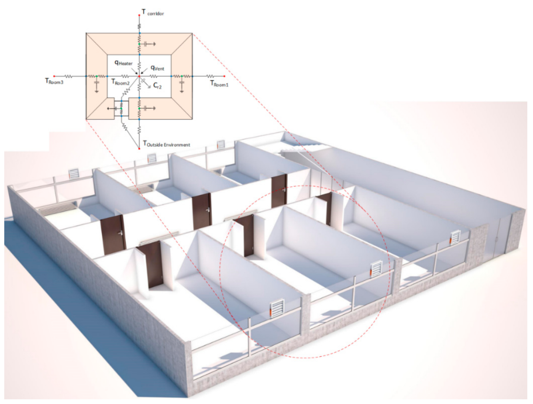
The rest of the paper is organized as follows. Section 2 presents the system model, while Section 3 describes the diagnostic algorithm based on a fuzzy Bayesian belief network. The implementation of the method based on the use case of DCV and heating systems is shown in Section 4. Section 5 presents the evaluation results and discussion, and the conclusion is described in the last section of this paper.

2. System Model

This section explains the system model of a DCV and heating system that tests the diagnostic methodology. An understanding of the overall behavior of the system is required before applying any diagnosis technique through system model analysis. Analysis of the system model leads to knowledge about the system’s functionality. The function of a system is what the system is intended to do [32], whereas the model specifies what a system does [33]. The methodology in this paper is introduced based on the DCV and heating system model as an example scenario of the modern HVAC systems with their numerous components. In this model, embedded processing units orchestrate the nodes of Wireless Sensors and Actuators Networks (WSANs) with the physical environment to adaptively control the air quality and temperature of an office building. The system model of the HVAC systems includes a typical building with several rooms on different floors, for example, an example office building with six rooms and a corridor equipped with a DCV and heating system. Each room is generally occupied by several components, for example, sensors or actuators. The thermal dynamics of the system model must be established. For example, the lumped-capacitance method has been used in this paper to model the thermal dynamics of the use-case office building (thermal network model) where the heat transfer is illustrated by thermal resistance and heat storage (thermal capacitance). In this model, each zone and each wall are represented by a thermal node. The nodes are connected via thermal capacitors to the ground reference and thermal resistors to the adjacent nodes. In the designed model of this study, for every zone, there is a central node that is later connected to central nodes of other zones via thermal paths across the walls and windows. A schematic of this node and its connections can be seen in the Figure 1 and Figure 2.

Figure 1. Schematic of the equivalent lumped capacitance model for a standard room.

Figure 2. Schematic of the equivalent lumped-capacitance model for an office building with six rooms and one corridor.

The DCV is a control strategy based on ventilation to modify the amount of fresh air to improve the indoor air quality while increasing the potential energy saving by automatic adjustment of the volume of air exchange using damper actuators based on sensor values received from air quality sensors, for example, CO₂ concentration sensors, temperature sensors, occupancy sensors, heater status, and control theory. Figure 3 shows the role of the DCV and heating system in optimizing the system considering different parameters.

Figure 3. Role of DCV and heating system in optimizing the system.

The model considers the heating and ventilation (not the cooling) because the model studies the winter season when the range of outdoor temperature is below the range of acceptable indoor temperature. Figure 4 shows an office building sketch for the system model. The model is developed based on thermal dependencies among different zones and the environment during a typical winter day in February. Behravan et al. described the model dynamics in [34]. The differential balance equations for each node have been solved with an explicit numerical method.

Figure 4. Office building sketch [34].

This paper shows the cluster-tree-mesh topology based on the building architecture that supports wireless and battery-powered nodes (devices) with minimum routing efforts in Figure 5 [35]. The sensor nodes in each zone send the measured values, for example, temperature, occupancy, or CO₂ concentration, to the cluster head of the router zone. The router receives the values and forwards them to the controller via the coordinator. After calculations, the controller processes the received values, determines the commands, and exerts them on the actuators, for example, heater and damper actuator, which is finally applied to the plant.

Figure 5. Network topology based on building architecture [30].

Faults are inevitable events that affect the components, the system’s functionality, and performance. Faults may lead to a system-level or component-level failure or malfunction if they are not detected and mitigated. Failures can involve performance degradation, safety risks, and excess cost, and energy waste. From the time perspective, faults may occur during the whole operation of the system as a permanent fault or may be limited to a specific period as an intermittent fault. Faults with time dependency can be categorized into abrupt faults (stepwise/short), incipient faults, constant faults, noisy faults, and intermittent faults [36]. Constant faults arise when a sensor reports a constant value over time instead of the real and normal sensor values or when an actuator is stuck at a constant position. Faults can affect components such as sensors, actuators, and computational nodes, and communication networks. Faults in actuators may lead to loss of controllability. In sensors, they can affect reliable measurement information, and in the computational nodes, faults will change the behavior of the entire plant.

In this paper, the following component faults are used for the diagnostic algorithm introduced. The faults are modeled based on the measured values from the sensors such as temperature sensors, CO₂ concentration sensors, and command or status values in actuators, for example, heater actuators (thermostats) and damper actuators. These faults are constant-valued or stuck-at faults, as listed below.

• CO₂ Sensor Fault: The CO₂ sensor fault represents a wrong sensor reading as a constant or noisy value. For example, a constant value of 700 ppm or noisy values within the range of a subdomain from all the subdomains of a domain or attribute. However, this paper assumed the constant fault;
• Temperature Sensor Fault: This type represents a wrong sensor reading with a constant value, for example, 15 °C;
• Damper Actuator Fault: This type of fault represents a stuck-at fault where a damper is stuck at a specific position. For example, if the damper is stuck at its open position, it gets the binary value 1, which means excess low-temperature fresh air comes inside. Therefore, the inside temperature will decrease, and the heater must constantly work to compensate for the heat loss. If the damper is stuck at its closed position, then it gets the value 0, which means that the inside air temperature will increase, and the indoor CO₂ concentration will pass the maximum permitted limit;
• Heater Actuator (Thermostat) Fault: This type of fault represents a stuck-at fault where the heater sticks at a specific position. For example, if the heater is stuck at its ON position, it gets the value 1, which means inside air temperature increases. If the heater is stuck at its OFF position, it gets the binary value 0, which means the inside, air temperature tends to decrease.

The equation that describes the generated data from a sensor and actuator node can be modeled as a function concerning time f(t) [37], as can be seen:

$$f(t)=x,$$

(1)

where f(t) represents the value sensed by the node at the time $t$, $x$ is the non-faulty sensor value at the time t, knowing that in the real world, there is no ideal signal. Therefore, the noise $n$ will be added to Equation (1). As a result, this equation can be written as the following:

$$f(t)=x+n.$$

(2)

Some factors are added to normalize Equation (2); for instance, $A,B,n$ are factors that can be used to determine the fault type, where A is the multiplicative constant and called gain, whereas B is the additive constant and called offset, and n is the external noise. According to the above, the general form of this equation can be seen here:

$$f(t)=Ax+B+n.$$

(3)

Four different types of faults are modeled as examples, gain fault, offset fault, noise fault, and stuck-at fault. Stuck-at-fault can be defined as faulty data that has a constant value. The variance of the measured values from the fault occurrence is zero in the stuck-at fault, and the sensed data shows a constant value $A=0,B\ne 0,n=0$.

$$f(t)=B.$$

(4)

A further detailed expression of the established DCV and heating system model, faults models, and fault hypotheses are described by Behravan et al. in [30,34,38,39].

3. Diagnostic Classifier Based on FBBN

This section cuts through the generic steps of the combined diagnostic classifier to diagnose any stuck-at or constant faults based on the causal relation in a fuzzy Bayesian belief network using the relation direction probabilities. The result of FBBNs that are causal relationships is then visualized using the graphs and table of listing based on RDPs. The graphs are constructed from nodes (indices) and edges (arcs). Figure 6 shows the direction of the arcs with the direction of the dependency between each pair of nodes based on the conditional probability values extracted from the Conditional Probability Table (CPT). Fuzzy association rules are calculated from the network and weights of the relationship between two nodes are assumed as confidence factor of these rules.

Figure 6. Causal relationships indicated by the graphs.

This section shows the steps of the generic automatic diagnostic algorithm as a classifier that is introduced in this paper. Different steps are data preparation, system attributes and subdomains definitions, fuzzy theory and generating weighted fuzzy data over relational data table, probability of subdomains using fuzzy theory, intersection probability MI theory, finding direction and probability of transitions using conditional probabilities, and fault diagnosis. Figure 7 shows the scheme of a diagnostic classifier based on causal relations in FBBNs using RDPs.

Figure 7. Scheme of a diagnostic classifier based on causal relations in FBBNs using RDPs.

3.1. Data Preparation

In the first step, a Relational Data Table (RDT) of all random variables of the system is created as a basis of the recorded data that must be used for the fault diagnosis. The data samples include information about all variables or attributes as tuples [20]. A fault injection framework is a helpful tool for studying the behavior in the presence of faults and evaluating diagnostic techniques. Diagnostic techniques can serve for triggered appropriate recovery actions to achieve an acceptable level of service despite occurring faults. Considering the vast range of diagnostic methods, establishing an accurate diagnostic model that maps system failures to the correct faults is a time-consuming task that may involve extensive try-and-error efforts [34]. In this paper, fault injection is used as a technique to determine the coverage of the fault diagnosis by producing faults in the system in order to trace the behavior of the system in existence or absence of different kinds of faults and evaluate their effect by monitoring several parameters, for example, energy consumption and occupancy comfort. Table 2 shows the samples with their attributes’ values over time.

Table 2. Relational Data Table (RDT).

Samples	Attribute1	Attribute2	Attribute3	Attributem
S1	Value11	Value12	Value13	Value1m
S2	Value 21	Value 22	Value23	Value2m
Sn	Valuen1	Valuen2	Valuen3	Valuenm

In this table, RDT = {S₁, S₂, S₃, …, S_n}, where S_i is the data sample as a tuple of values for the i-th time instance. S_i = {Value_i1, Value_i2, …, Value_im}, where the values are captured the information for each sample time. Attribute or domain is variable with its measured values over time.

3.2. System Attributes and Subdomain Definitions

A domain is a set of ranged values for a variable, where this vast range can be divided into small ranges as a set of subdomains. Figure 8 shows a sample domain with its subdomains with the values along the Y-axis over time along the X-axis.

Figure 8. An example domain and its subdomains.

Attribute-ith = {Subdomain₁, Subdomain₂, …, Subdomain_p}, where subdomains can be a subset of continuous or discrete values.

In this step, the attributes will be classified into several subdomains. This classification can be done using the fuzzy theory [15]. The values with continuous changes will be classified using the fuzzy functions, while those with discrete changes will be classified based on their discrete values. Once all the attributes were classified into subdomains, the Subdomain Label Table (SLT) is generated that includes all attributes and their subdomains. Table 3 indicates the SLT. All the subdomains of each attribute will then be saved in the Subdomain Label Vector (SLV). SLV is a vector of all the subdomains extracted from the SLT table.

Table 3. Subdomain Label Table (SLT).

No.	Attributes	Subdomains	Subdomains	Subdomains
1	Attribute1	Subdomain11	Subdomain12	Subdomain1n
2	Attribute2	Subdomain21	Subdomain22	Subdomain2e
n	Attributen	Subdomainn1	Subdomainn2	Subdomainnf

3.3. Generating Weighted Fuzzy Data Based on Fuzzy Theory

Once the subdomains are defined, the probability of each subdomain as weight (W) is calculated based on the Membership Degree (MD) using the Membership Function (MF). The MF obtains the value and produces MD values with a range of [0, 1]. There are various types of fuzzy membership functions: triangular, trapezoidal, Gaussian, and bell-shaped membership functions. The Trapezoidal has been used in this paper as follows.

$$Degree\hspace{0.33em}of\hspace{0.33em}Membership(x:a,b,c,d)=\left\{\begin{array}{c}0\hspace{1em}\hspace{1em}\hspace{1em}x<a\\ \frac{(x-a)}{(b-a)}\hspace{1em}a\le x\le b\\ 1\hspace{1em}\hspace{1em}\hspace{1em}b\le x\le c\\ \frac{(d-x)}{(d-c)}\hspace{1em}c\le x\le d\\ 0\hspace{1em}\hspace{1em}\hspace{1em}x\ge d\end{array}\right.$$

(5)

Table 4 shows the MD values or W values (weights) extracted from Equation (5) for different subdomains in a table called Weighted Fuzzy Relational Data Table (WFRDT) based on the values in Table 1. All weights of all samples for each subdomain are summed up to calculate the total weight for each subdomain. The total weight is placed in the last row of the WFRDT table.

Table 4. Weighted Fuzzy Relational Data Table (WFRDT).

	Attribute1				Attribute2
No. of Records	Subdomain11	Subdomain12	…	Subdomain1m	Subdomain21	Subdomain22	…	Subdomain2e
1	W11	W12	…	W1m	W11	W12	…	W1e
2	W21	W22	…	W2m	W21	W22	…	W2e
…	…	…	…	…	…	…	…	…
n	Wn1	Wn2	…	Wnm	Wn1	Wn2	…	Wne
Total Weight	$W_1={\displaystyle \sum _{11}^{n1}W}$	$W_2={\displaystyle \sum _{12}^{n2}W}$	…	$W_m={\displaystyle \sum _{1m}^{nm}W}$	$W_1={\displaystyle \sum _{11}^{n1}W}$	$W_2={\displaystyle \sum _{12}^{n2}W}$	…	$W_e={\displaystyle \sum _{1e}^{ne}W}$

3.4. MI and Probability of Subdomains

MI is a concept rooted in information and probability theory. MI of two random variables is a statistical measurement of the mutual dependence of two random variables [20]. MI measures information about one random variable by observing the other random variables [40]. There are many definitions of random variables. For example, G. Zeng [41] has classified MI definitions into two categories: (1) definitions with random variables and (2) ensembles. The fuzzy theory can be used as an appropriate likelihood density function [42]. Intan et al. [20] defined the MI between two fuzzy sets of A and B as follows

$$MI(A,B)=MI(B,A)=P(A,B){\log }_2\left(\frac{P(A,B)}{P(A)\times P(B)}\right),$$

(6)

where $P(A)\ne 0$ and $P(B)\ne 0$. P(A) and P(B) are the probability values of fuzzy sets A and B, and P(A,B) is the joint probability value of fuzzy sets A and B or the intersection between A and B. The equation above determines a correlation measure, that is, MI(A,B) > 0 refers to a positive correlation that describes the fuzzy sets A and B have a relationship in constructing a network.

$$P(A)=\frac{{\displaystyle \sum _{k=1}^{\left|R\right|}A(d_{kj})}}{\left|n\right|}\hspace{1em}and\hspace{1em}P(B)=\frac{{\displaystyle \sum _{k=1}^{\left|R\right|}B(d_{ki})}}{\left|n\right|},$$

(7)

where R is the number of records and $A(d_{kj}),B(d_{ki})\in [0,1]$ are membership degrees of d_kj and d_ki for fuzzy sets A and B, respectively [20]. The probability of the subdomains, that is, P(A), P(B), therefore can be measured by the total weights and using the Equation (8), where n is the number of samples (No. of Records). Table 5 shows the Subdomain Probability Vector (SPV).

$$P(Subdomai{n}_i)=\frac{{\displaystyle \sum _1^{n}Weights}}{\left|n\right|}.$$

(8)

Table 5. Subdomain Probability Vector (SPV).

	Attribute1			Attribute2
Subdomains	Subdomain11	Subdomain12	Subdomain1m	Subdomain21	Subdomain22	Subdomain2e
Probability of Subdomain	$P_1=\frac{W_1}{n}$	$P_2=\frac{W_2}{n}$	$P_m=\frac{W_m}{n}$	$P_1=\frac{W_1}{n}$	$P_2=\frac{W_2}{n}$	$P_e=\frac{W_e}{n}$

3.5. Joint (Intersection) Probability

A joint probability is a statistical measurement for two events occurring at the same time instance. If event A changes the probability of event B, then they are dependent; otherwise, they are independent. The probability value for the independent events is equal to zero. Therefore, the dependent events are determined. In this paper, to calculate the dependent subdomains, the algorithm compares the fuzzy weights of each time sample in pairs of different subdomains and different attributes to find the minimum weight value of that pair. Finally, the algorithm calculates the intersection (joint) probability of that pair (of subdomains), respectively. The algorithm generates a triangular top matrix of intersection (joint) probabilities of subdomains called Intersection Triangular Top Matrix (ITTM). Therefore, if P(A,B) is the probability of two subsets A and B, the Intersection probability is calculated using the following equation [20]:

$$P(A,B)=P(A\cap B)=\frac{{\displaystyle \sum _{k=1}^{\left|R\right|}\min \left(A(d_{kj}),B(d_{ki})\right)}}{\left|R\right|}=\frac{{\displaystyle \sum _1^n\min \left(A(WSubdomai{n}_i),B(WSubdomai{n}_j)\right)}}{n}$$

(9)

Here, A(WSubdomain_i) and B(WSubdomain_j) are the fuzzy weights of subdomains A and B. Note that P(A,B) is equal to P(B,A); therefore, this is not essential to measure both the top and down triangular. In this paper, we only consider the values of the top triangular matrix. Table 6 describes the Intersection Triangular Top Matrix (ITTM).

Table 6. Intersection Triangular Top Matrix (ITTM) (To show that the algorithm only deals with upper side of the matrix which is highlighted in grey color).

	Subdomains	1	2	3	4	5	6	7	8	9	10	11	12	13	14	15	…	i-1	i
Subdomains
1
2										P(2,9)
3
4
5
6
7													P(7,12)
8
9
10
11
12
13																P(13,15)
14
15
…
i-1
i

3.6. Subdomains’ Relation Using MI

After calculation of P(A), P(B), and P(A,B) for all subdomain pairs, Equation (6) will get the value for the MI. The positive MI value shows a dependency between two subdomains of a pair, and the negative MI value indicates independent subdomains of a pair. The diagnosis algorithm in this paper assumes the binary value of 1 for the positive MI values and the binary value of 0 for the negative MI values. The binary results will then be placed in a top triangular matrix named Subdomains Relation Table (SRT) as shown in the Table 7.

Table 7. Subdomains Relation Table (SRT) (To show that the algorithm only deals with upper side of the matrix which is highlighted in grey color).

	Subdomains	1	2	3	4	5	6	7	8	9	10	11	12	13	14	15	16	…	i
Subdomains
1
2
3									1				1					1
4											1
5
6															1
7
8												1
9																1		1
10
11
12
13																	1
14
15
16
…
i

3.7. Conditional Probability

In this step, the conditional probabilities are measured. The conditional probabilities of fuzzy event A given B are denoted by P(A|B) [20].

$$P(A\mid B)=\frac{P(A,B)}{P(B)}=\frac{{\displaystyle \sum _{k=1}^{\left|R\right|}\min \left(A(d_{kj}),B(d_{ki})\right)}}{{\displaystyle \sum _{k=1}^{\left|R\right|}B(d_{ki})}}.$$

(10)

This P(A|B) corresponds to P(subdomain_i | subdomain_j) in the method described in this paper.

$$P(subdomai{n}_i\mid subdomai{n}_j)=\frac{{\displaystyle \sum _1^n\min \left(A(WSubdomai{n}_i),B(WSubdomai{n}_j)\right)}}{{\displaystyle \sum _1^{n}B(WSubdomai{n}_j)}}.$$

(11)

The conditional probabilities of fuzzy event B given A are also denoted by P(B|A) [20].

$$P(B\mid A)=\frac{P(B,A)}{P(A)}=\frac{{\displaystyle \sum _{k=1}^{\left|R\right|}\min \left(A(d_{kj}),B(d_{ki})\right)}}{{\displaystyle \sum _{k=1}^{\left|R\right|}A(d_{kj})}}.$$

(12)

The above equation corresponds to P(subdomain_j | subdomain_i) in the method described in this paper.

$$P(subdomai{n}_j\mid subdomai{n}_i)=\frac{{\displaystyle \sum _1^n\min \left(A(WSubdomai{n}_i),B(WSubdomai{n}_j)\right)}}{{\displaystyle \sum _1^{n}A(WSubdomai{n}_i)}}.$$

(13)

The results from the above equations will be stored in a matrix called the Conditional Probabilities Table (CPT) shown in Table 8 with the following rules:

Table 8. Conditional Probabilities Table (CPT) (The background color to show the diameter of the matrix which is highlighted in white color).

	Subdomains	1	2	3	4	5	6	7	8	9	10	11	12	13	14	15	16	17	18
Subdomains
1
2										P(Subdomain2|Subdomain9)
3
4
5
6
7
8
9			P(Subdomain9|Subdomain2)
10
11
12
13
14
15
16
17
18

• P(A|B) > P(B|A) indicates the direction of dependency between A and B is from B to A. Then, P(B|A) will be eliminated, and P(A|B) will be stored in Table 8.
• P(B|A) > P(A|B) indicates the direction of dependency between A and B is from A to B. Then, P(A|B) will be eliminated, and P(B|A) will be stored in Table 8.

In Table 8, the highlighted elements of the matrix with the yellow color show the conditional probability of each pair of subdomains, for example, P(Subdomain₉|Subdomain₂) and P(Subdomain₂|Subdomain₉). Then, the conditional probability with the higher value will be kept and saved in the CPT table as the green elements of the matrix, and the conditional probability with the lower value will be deleted from the CPT table.

3.8. Relation-Direction Probabilities

Relation Direction Probabilities (RDPs) in Table 9 indicate all the relations and their features, that is, the direction between dependent subdomains and the conditional probability of the transmission. The RDP table includes the parents’ and children’s columns generated based on the subdomains and the conditional probabilities of these pairs listed in the CPT table.

Table 9. Relation Direction Probability (RDP).

Number of Relations	Parents	Children	Conditional Probabilities
1	Subdomaini	Subdomainj	P(Subdomainj | Subdomaini)
2	Subdomaink	Subdomainw	P(Subdomainw | Subdomaink)
n	Subdomainn	Subdomainm	P(Subdomainm | Subdomainn)

All existing elements in the CPT table are ordered in this table in which the conditional probability of P (Subdomain_j | Subdomain_i) presents that there is a relation between Subdomain_j and Subdomain_i and the direction is from Subdomain_i (Parent Node) to Subdomain_j (Child Node) with the probability of P(Subdomain_j | Subdomain_i).

3.9. Causal Relation in FBBN Using the Relation Direction Probabilities

As mentioned, the FBBN shows the causal relationships between each pair of subdomains that are extracted from the RDP table. The conditional probabilities indicate the direction of the dependency in each pair of nodes. Figure 9 is an example that shows Subdomain_j (Child Node) is related to Subdomain_i (Parent Node).

Figure 9. Causal relation in FBBN using the relation direction probabilities.

3.10. Fault Diagnosis Classification Based on Causal Relations in FBBNs

The research in this paper shows that the FBBN causal relation based on the RDPs can determine all the cause-effect relationships among every subdomain in case of faults. Therefore, the authors used this capacity to diagnose stuck-at fault types for several components with various stuck-at values at different time instances. This research considers the constant faults because the constant values will be in a subdomain from a whole range of values for a parameter. Therefore, the diagnosis method can correlate the faulty value with the fault. In this section, an overview of the overall methodology is described.

This diagnosis method has two modes: the online mode and the offline mode. The offline mode includes the generation phase of the reference libraries, including various faulty conditions (fault objects) for diagnosing different real fault cases with random/real faulty values. Figure 10 indicates an overview of the fault diagnosis method introduced in this paper based on the causal relations in FBBNs using the relation direction probabilities.

Figure 10. Overview of fault diagnosis based on the causal relations in FBBNs using the relation direction probabilities.

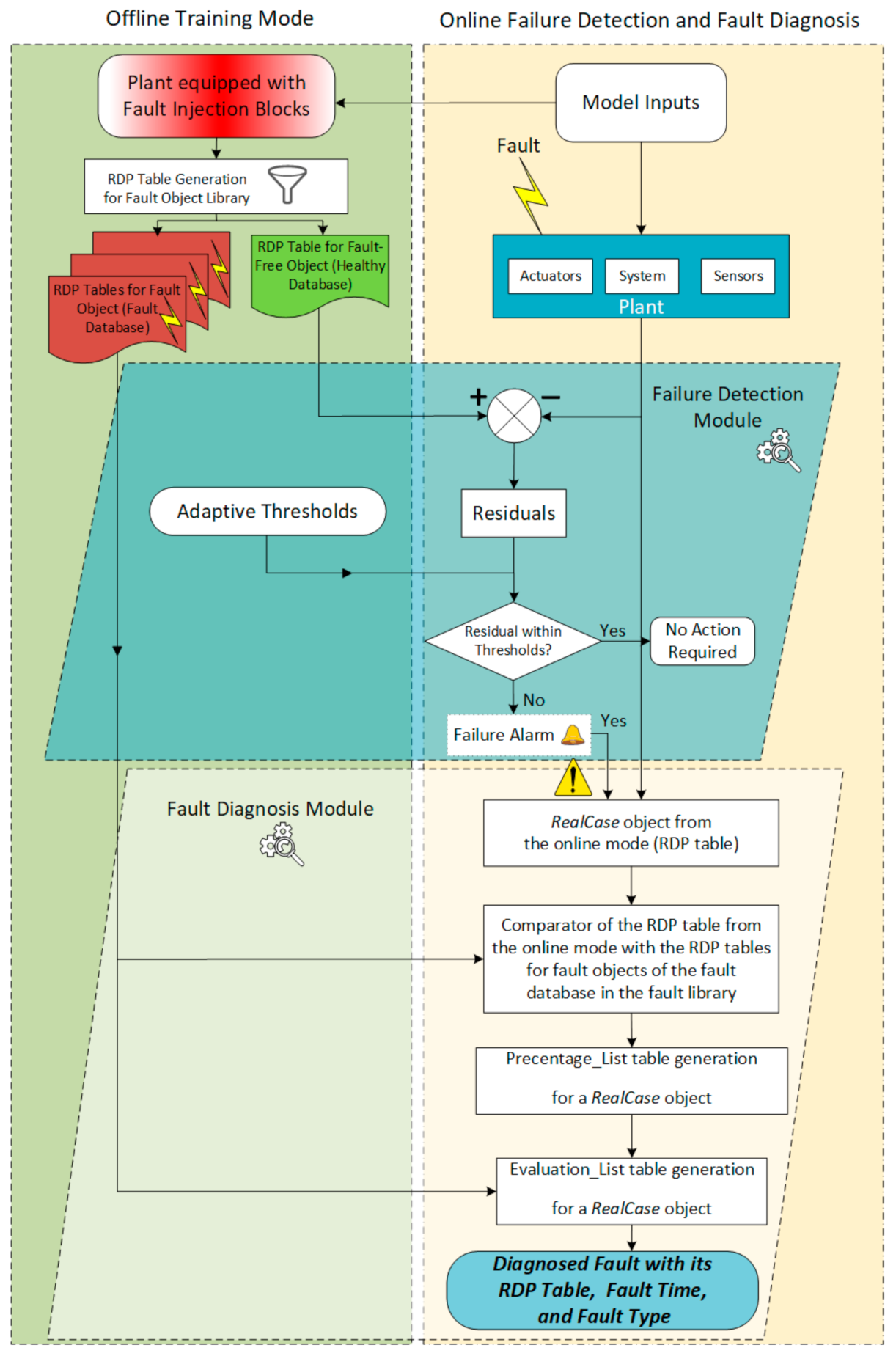
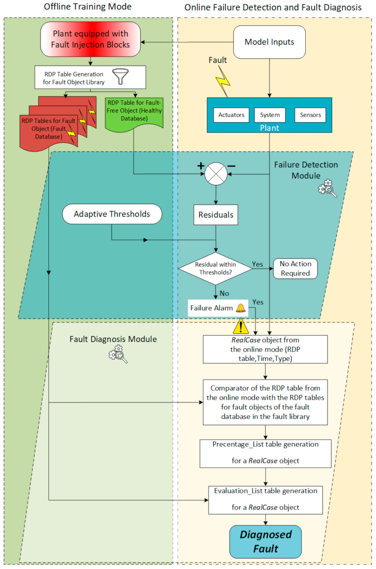
3.10.1. Offline Training Mode

The offline training mode includes a library of different fault modes. In this library, a fault object for each type of fault is created that is named: Fault_Object_i, i = {1, n}. The n value depends on the total number of subdomains (p) and the time vector (t). Table 10 shows an overview of the offline library of the fault cases. The fault object is defined as a class in MATLAB as function (1) that contains four properties: type of fault (Type), time of fault injection (Time), the system parameters’ values for each fault case (Data), and the RDP table. This library is generated for every fault type that includes all subdomains of a domain and for different fault injection times. To include all the subdomains, a representative for each subdomain and for each time interval is defined. The time interval is a vector of time values for the total time domain.

Table 10. Offline library of fault cases.

No. of Faults	1	2	3	n-1	n
Objects for Different Fault cases	Fault_Object1	Fault_Object2	Fault_Object3	Fault_Objectn-1	Fault_Objectn

Function 1. Fault Class Definition

classdef Fault

properties

Type;

Time;

Data;

RDP;

end

end

3.10.2. Online Diagnostic Mode

The online mode represents the real case scenario simulated in this research using the fault injection framework. Time, type, and value in this fault injection are the properties of the real scenario with random values within a range. The RDP table in the online mode contains all the relations of subdomains of the real case (RealCase). For the diagnosis of the real case, the RealCase Diagnosis Class is defined in Function 2 with three properties, including Type, Time, and Value of random case. This class also includes two more properties: Percentage_List and Evaluation_List.

Function 2. RealCase Diagnosis Class Definition

classdef RealCase Diagnosis

properties

Type;

Time;

Value;

Percentage_List; // the size of this list is equal to n or the number of fault cases in the offline library

Evaluation_List; // The size of this list is equal to x

end

end

The result from the function above for fault case_i will be stored in the element_i of a list called Percentage_List. This list includes n number of percentages of similarity for a RealCase compared to the n fault objects in the offline library. Table 11 shows the Percentage_List for a RealCase object. After that, the x number of top-ranked similar fault cases based on the highest percentages in the Percentage_List will be distinguished by the diagnosis algorithm as the most relevant results, stored in the Evaluation_List.

Table 11. Percentage_List for a RealCase object.

No. of Fault Object in the Offline Library	1	2	…	i
Calculated Percentage of Similarity between the RealCase fault object and each Fault Object in the Offline Fault Library	Percentage of Similarity1	Percentage of Similarity2	…	Percentage of Similarityi

The evaluation list in Table 12 consists of x elements, and every element j (1 < j < x) has three properties: type, time, and percentage. The type and the time are allocated from the fault case_i in the offline library. The percentage is the percentage of similarity that is actually the belief and the larger the fault belief means the higher the possibility of the corresponding fault. The diagnosis algorithm sorts the evaluation list by the rank order of values in the percentage column. “ranking” in statistics is the data transformation that the number or order of values are justified by their rank when they are sorted. Therefore, the elements with the higher percentages of similarity will be placed at the top ranks, and the lower percentages of similarity will be placed at the lower ranks.

Table 12. Evaluation_List for a RealCase object.

No.	Type	Time	Percentage
1	Offline_FaultType1	Offline_FaultTime1	Highest_Percentage1
2	Offline_FaultType2	Offline_FaultTime2	Highest_Percentage2
3	Offline_FaultType3	Offline_FaultTime3	Highest_Percentage3
j	Offline_FaultTypej	Offline_FaultTimej	Highest_Percentagej

The type and time of element j of this list are the type and time of the fault case_i object in the offline library. Finally, the comparison results of the type and the time values of the Evaluation_List with the type and the time of the RealCase object which can determine the belief of the fault diagnosis method in this paper based on the causal relation in fuzzy Bayesian belief network using the relation direction probabilities.

4. Implementation of the Diagnostic Classifier Based on the Example System Model

As mentioned in Section 3.10.2, the RDP tables are the primary data required for the online diagnosis phase. This section describes an example scenario for the introduced diagnostic method in Section 3 for a DCV and heating system use-case in MATLAB/Simulink. Here, an example fault type is selected in the DCV and heating system model’s fault injection framework to show the diagnosis methodology’s detailed description. The selected fault type is the CO₂ sensor fault with a stuck-at value of 700 ppm with the fault injection time of 18,000 s. The simulation is run for 86,400 s or one typical winter day.

4.1. Data Preparation in System Model

The Data Preparation step includes extracting the data from signal values of Simulink-Model and initializing the RDT table. An output from the system model in MATLAB/Simulink prepares RDT required for the introduced diagnosis methodology in this paper. An example RDT based on the DCV and heating system model is shown in Table 13. The attributes can be domains with continuous or discrete values. In this table, the samples for 86,400 s or one-day simulation time can be recorded. Therefore, RDT = {S₁, S₂, S₃, …, S₈₆₄₀₀}.

Table 13. Use-case RDT for CO₂ sensor fault in 18,000 s Fault (The Background color shows the fault injection time sample).

Seconds (Samples)	Daily Temperature	Occupancy Number	Room Temperature	Room CO2 Concentration	Heater Status	Damper Status
1	7.0004	0	19.9905	400	0	0
2	7.0007	0	19.9810	400	0	0
3	7.0011	0	19.9715	400	0	0
4	7.0015	0	19.9620	400	0	0
5	7.0018	0	19.9525	400	0	0
…	…	…	…	…	…	…
17,999	11.8293	6	19.5583	579.0654	1	1
18,000	11.8294	6	19.5570	700	1	1
18,001	11.8295	6	19.5556	700	1	1
18,002	11.8296	6	19.5543	700	1	1
18,003	11.8297	2	19.5530	700	1	1
…	…	…	…	…	…	…
86,399	6.9996	0	16.8578	700	1	1
86,400	7	0	16.8581	700	1	1

4.2. Attributes and Subdomains Preparation in System Model

Attributes and subdomains preparation step includes defining the labels of attributes and subdomains of the system for analysis and defining fuzzy sets over these attributes.

4.2.1. Attributes in System Model

For defining attributes, they are first divided into two types—continuous and discrete. The continuous attributes have continuous changes in their values, such as room temperature, daily temperature, room CO₂ concentration, and occupancy parameters. The discrete attributes are heater status and damper status. There is also a simulation clock as a discrete attribute required for the evaluation step.

4.2.2. Subdomains in System Model

Once the continuous and discrete attributes and subdomains were defined in the previous section, the SLT table is created, shown in Table 14. The subdomains are also named nodes. For example, subdomains for the continuous daily temperature attribute are three subdomains of low daily temperature, middle daily temperature, and high daily temperature. These subdomains are used to create the fuzzy sets for the fuzzy function. Eighteen subdomains based on seven attributes can facilitate the conditional probability measurement of the BBN. The subdomain index is considered as a reference to the subdomain title. Table 14 shows three example subdomains for the attribute of room temperature. Figure 11 illustrates the subdomains and fuzzy sets for room temperature signal.

Table 14. Use-case SLT.

No.	Attributes	Subdomains	Subdomains	Subdomains
1	Daily Temperature	Low_Daily_Temperature (No. 1)	Middle_Daily_Temperature (No. 2)	High_Daily_Temperature (No. 3)
2	Occupants Number	Low_Occupancy (No. 4)	Normal_Occupancy (No. 5)	High_Occupancy (No. 6)
3	Room Temperature	Lower_than_Threshold_ RoomTemperature (No. 7)	Within_Threshold_ RoomTemperature (No. 8)	Upper_than_Threshold_ RoomTemperature (No. 9)
4	Heater Status	Heater_Status_On (No. 10)	Heater_Status_Off (No. 11)	---------
5	Damper Status	Damper_Status_Open (No. 12)	Damper_Status_Close (No. 13)	---------
6	Simulation Clock	Healthy_Mode (No. 14)	Faulty_Mode (No. 15)	---------
7	Room CO2 Concentration	Lower_than_Threshold_CO2Value (No. 16)	Within_Threshold_CO2Value (No. 17)	Upper_than_Threshold_CO2Value (No. 18)

Figure 11. Illustration of subdomains and fuzzy sets definitions for room temperature.

4.3. Fuzzy Rules in System Model

In this section, fuzzy rules or membership functions are defined to generate the probability weights based on the MD values from the fuzzy function. The conditional probability of each subdomain will be measured by the MD of each sample of the subdomain through the following steps.

4.3.1. Fuzzy Membership Functions

In this section, the fuzzy membership functions that get the MD value for each x input value are explained.

Room Temperature Fuzzy Membership Function

The total range of the room temperature has been considered between [0–40]. This range can be divided into three subdomains of low room temperature with a [0–17.5] range, middle room temperature with a [17.5–22.5] range, and high room temperature with a [22.5–40] range. Twenty degrees centigrade is the nominal temperature value of the system. Equations (17)–(19) show the fuzzy membership functions respective to each subdomain. Figure 12 shows the overall room temperature fuzzy membership function with the related fuzzy function of each subdomain in three various colors of blue for low temperature values, green for middle-temperature values, and red for high-temperature values.

$$Low\_Room\_Temperature\_Fuzzy\_Membership\_Function(x)=\left\{\begin{array}{c}1\hspace{1em}\hspace{1em}\hspace{1em}x\le 17.5\\ \frac{(19.5-x)}{(19.5-17.5)}\hspace{1em}17.5\le x\le 19.5\\ 0\hspace{1em}\hspace{1em}\hspace{1em}x\ge 19.5\end{array}\right.$$

(14)

$$Middle\_Room\_Temperature\_Fuzzy\_Membership\_Function(x)=\left\{\begin{array}{c}0\hspace{1em}\hspace{1em}\hspace{1em}x<17.5\\ \frac{(x-17.5)}{(19.5-17.5)}\hspace{1em}17.5\le x\le 19.5\\ 1\hspace{1em}\hspace{1em}\hspace{1em}19.5\le x\le 20.5\\ \frac{(22.5-x)}{(22.5-20.5)}\hspace{1em}20.5\le x\le 22.5\\ 0\hspace{1em}\hspace{1em}\hspace{1em}x\ge 22.5\end{array}\right.$$

(15)

$$High\_Room\_Temperature\_Fuzzy\_Membership\_Function(x)=\left\{\begin{array}{c}0\hspace{1em}\hspace{1em}\hspace{1em}x<20.5\\ \frac{(x-20.5)}{(22.5-20.5)}\hspace{1em}20.5\le x\le 22.5\\ 1\hspace{1em}\hspace{1em}\hspace{1em}x\ge 22.5\end{array}\right.$$

(16)

Figure 12. Room temperature fuzzy membership functions.

Daily Temperature Fuzzy Membership Function

The total range of the daily temperature has been considered between [0–14]. This range is divided into three subdomains: the low daily temperature with [0–5] range, middle daily temperature with [5–9] range, and high daily temperature with [9–14] range. Below, the fuzzy membership functions are shown and their illustration is in Figure 13.

$$Low\_Daily\_Temperature\_Fuzzy\_Membership\_Function(x)=\left\{\begin{array}{c}1\hspace{1em}\hspace{1em}\hspace{1em}x\le 5\\ \frac{(6.825-x)}{(6.825-5)}\hspace{1em}5\le x\le 6.825\\ 0\hspace{1em}\hspace{1em}\hspace{1em}x\ge 6.825\end{array}\right.$$

(17)

$$Middle\_Daily\_Temperature\_Fuzzy\_Membership\_Function(x)=\left\{\begin{array}{c}0\hspace{1em}\hspace{1em}\hspace{1em}\hspace{1em}x<5\\ \frac{(x-5)}{(6.825-5)}\hspace{1em}5\le x\le 6.825\\ \hspace{1em}\hspace{1em}1\hspace{1em}\hspace{1em}6.825\le x\le 7.175\\ \frac{(9-x)}{(9-7.175)}\hspace{1em}7.175\le x\le 9\\ 0\hspace{1em}\hspace{1em}\hspace{1em}x\ge 9\end{array}\right.$$

(18)

$$High\_Daily\_Temperature\_Fuzzy\_Membership\_Function(x)=\left\{\begin{array}{c}0\hspace{1em}\hspace{1em}\hspace{1em}x<20.5\\ \frac{(x-7.175)}{(9-7.175)}\hspace{1em}7.175\le x\le 9\\ 1\hspace{1em}\hspace{1em}\hspace{1em}x\ge 9\end{array}\right.$$

(19)

Figure 13. Daily temperature fuzzy membership functions.

CO₂ Concentration Fuzzy Membership Function

The CO₂ concentration values are considered in a range of [0–1200]. The CO₂ concentration variable is divided into three subdomains of the low CO₂ concentration with [0–400] range, middle CO₂ concentration with [400–800] range, and CO2 concentration with [800–1200] range. Figure 14 illustrates the fuzzy membership function of the CO₂ concentration.

$$Low\_C{O}_2\_Concentration\_Fuzzy\_Membership\_Function(x)=\left\{\begin{array}{c}1\hspace{1em}\hspace{1em}\hspace{1em}x\le 400\\ \frac{(585-x)}{(585-400)}\hspace{1em}400\le x\le 585\\ 0\hspace{1em}\hspace{1em}\hspace{1em}x\ge 585\end{array}\right.$$

(20)

$$Middle\_C{O}_2\_Concentration\_Fuzzy\_Membership\_Function(x)=\left\{\begin{array}{c}0\hspace{1em}\hspace{1em}\hspace{1em}\hspace{1em}x<400\\ \frac{(x-400)}{(585-400)}\hspace{1em}400\le x\le 585\\ \hspace{1em}\hspace{1em}1\hspace{1em}\hspace{1em}585\le x\le 615\\ \frac{(800-x)}{(800-615)}\hspace{1em}615\le x\le 800\\ 0\hspace{1em}\hspace{1em}\hspace{1em}x\ge 800\end{array}\right.$$

(21)

$$High\_C{O}_2\_Concentration\_Fuzzy\_Membership\_Function(x)=\left\{\begin{array}{c}0\hspace{1em}\hspace{1em}\hspace{1em}x<615\\ \frac{(x-615)}{(800-615)}\hspace{1em}615\le x\le 800\\ 1\hspace{1em}\hspace{1em}\hspace{1em}x\ge 800\end{array}\right.$$

(22)

Figure 14. CO₂ concentration fuzzy membership functions.

Occupancy Fuzzy Membership Function

The number of occupants in this system model differs in a range of [0–6] people based on an example scenario. An occupancy with less than three people in a day is considered low occupancy, with three and four people as middle occupancy, and with five and six people as high occupancy. These variations are illustrated in the fuzzy membership degree functions in equations below and Figure 15.

$$Low\_Occupancy\_Fuzzy\_Membership\_Function(x)=\left\{\begin{array}{c}1\hspace{1em}\hspace{1em}\hspace{1em}x\le 2\\ \frac{(3-x)}{(3-2)}\hspace{1em}2\le x\le 3\\ 0\hspace{1em}\hspace{1em}\hspace{1em}x\ge 3\end{array}\right.$$

(23)

$$Middle\_Occupancy\_Fuzzy\_Membership\_Function(x)=\left\{\begin{array}{c}0\hspace{1em}\hspace{1em}\hspace{1em}\hspace{1em}x<2\\ \frac{(x-2)}{(3-2)}\hspace{1em}2\le x\le 3\\ \hspace{1em}\hspace{1em}1\hspace{1em}\hspace{1em}3\le x\le 4\\ \frac{(5-x)}{(5-4)}\hspace{1em}4\le x\le 5\\ 0\hspace{1em}\hspace{1em}\hspace{1em}x\ge 5\end{array}\right.$$

(24)

$$High\_Occupancy\_Fuzzy\_Membership\_Function(x)=\left\{\begin{array}{c}0\hspace{1em}\hspace{1em}\hspace{1em}x<4\\ \frac{(x-4)}{(5-4)}\hspace{1em}4\le x\le 5\\ 1\hspace{1em}\hspace{1em}\hspace{1em}x\ge 5\end{array}\right.$$

(25)

Figure 15. Occupancy fuzzy membership functions.

4.3.2. Weighted Fuzzy Relational Data Table Based on RDT

This step generates the WFRDT based on RDT for the use case CO₂ sensor fault shown in Table 15. For this, a matrix of 86,401 rows and 18 columns is created. An example fault type that is the CO₂ sensor fault with a stuck-at value of 700 ppm with an example fault injection time of 18.000 s is considered. Every column of the table is a subdomain and contains fuzzy weights for continuous attributes and normal weights of occurrence for discrete attributes. The fuzzy weights based on the output from MD functions for each sample are measured for each subdomain. Each sample is a measured data sample in every second of simulation time. In the last row of this table, the total weights over one column are calculated.

Table 15. Use-Case Weighted Fuzzy Relational Data Table for CO₂ Sensor Fault (The Background color shows the fault injection time sample).

	Attributes	Daily Temperature			Occupancy			Room Temperature			Heater Status		Damper Status		Simulation Clock		Room CO2 Concentration
	Subdomains	1	2	3	4	5	6	7	8	9	10	11	12	13	14	15	16	17	18
No. Samples
1		0	1	0	1	0	0	0	1	0	0	1	0	1	1	0	1	0	0
2		0	1	0	1	0	0	0	1	0	0	1	0	1	1	0	1	0	0
3		0	1	0	1	0	0	0	1	0	0	1	0	1	1	0	1	0	0
4		0	1	0	1	0	0	0	1	0	0	1	0	1	1	0	1	0	0
5		0	1	0	1	0	0	0	1	0	0	1	0	1	1	0	1	0	0
…		…	…	…	…	…	…	…	…	…	…	…	…	…	…	…	…	…	…
17,999		0	0	1	0	0	1	0	1	0	1	0	1	0	0	0	0.0321	0.9679	0
18,000		0	0	1	0	0	1	0	1	0	1	0	1	0	0	1	0	0.5405	0.4595
18,001		0	0	1	1	0	0	0	1	0	1	0	1	0	0	1	0	0.54054	0.4595
18,002		0	0	1	1	0	0	0	1	0	1	0	1	0	0	1	0	0.54054	0.4595
18,003		0	0	1	1	0	0	0	1	0	1	0	1	0	0	1	0	0.54054	0.4595
…		…	…	…	…	…	…	…	…	…	…	…	…	…	…	…	…	…	…
86,399		0	1	0	1	0	0	1	0	0	1	0	1	0	0	1	0	0.54054	0.4595
86,400		0	1	0	1	0	0	1	0	0	1	0	1	0	0	1	0	0.54054	0.4595
Total Weight		37,133.7942	12,132.4114	37,133.7942	61,199	18,001	7200	53,381.5449	24,902.6097	8115.8453	85,676	724	73,790	12,610	18,000	68,400	6038.3843	48,643.6590	31,717.9565

4.4. Probability of Subdomains in System Model

As mentioned in Section 4.4, the probability of the subdomains can be measured by the total weights for each subdomain divided by the number of samples using the Equation (12). Therefore, the Subdomain Probability Vector (SPV) is calculated, and the result is shown in the Table 16.

Table 16. Use-Case Subdomain Probability Vector (SPV) for CO₂ Sensor Fault.

Attribute	Daily Temperature			Occupancy			Room Temperature			Heater Status		Damper Status		Simulation Clock		Room CO2 Concentration
Subdomain	1	2	3	4	5	6	7	8	9	10	11	12	13	14	15	16	17	18
Probability	0.4298	0.1404	0.4298	0.7083	0.2083	0.0833	0.6178	0.2882	0.0939	0.9916	0.0084	0.8541	0.1459	0.2083	0.7917	0.0699	0.5630	0.3671

4.5. (Intersection) Probability of Subdomain Pairs in System Model

In this step, a triangular top matrix is generated to store the intersection probabilities of subdomain pairs. The intersection probability of P(A,B) is equal to P(B,A). Therefore, it makes sense to calculate the probabilities upper than the main diagonal of the matrix. Therefore, Table 17 shows the following matrix with 18 rows and 18 columns using Equation (13).

Table 17. Use-case Intersection Triangular Top Matrix (ITTM) for CO₂ sensor fault (The background color is the boundary of the upper triangular matrix).

	Subdomains	1	2	3	4	5	6	7	8	9	10	11	12	13	14	15	16	17	18
Subdomains
1		0	0.0299	0	0.4298	0	0	0.4298	0	0	0.4298	0	0.4298	0	0	0.4298	0	0.2472	0.2123
2		0	0	0.0299	0.1053	0.0351	0	0.1076	0.0204	0.0249	0.136	0.0035	0.1053	0.0351	0.0351	0.1053	0.0351	0.0818	0.0707
3		0	0	0	0.1732	0.1732	0.0833	0.0828	0.2803	0.0792	0.4249	0.0049	0.3190	0.1108	0.1732	0.2566	0.0374	0.2812	0.1287
4		0	0	0	0	0	0	0.5069	0.1420	0.0594	0.7048	0.0035	0.6250	0.0833	0.0833	0.6250	0.0646	0.3565	0.2872
5		0	0	0	0	0	0	0.0917	0.0884	0.0282	0.2035	0.0049	0.1583	0.0501	0.0833	0.1250	0.0030	0.1455	0.0599
6		0	0	0	0	0	0	0.0193	0.0578	0.0063	0.0833	0	0.0708	0.0125	0.0417	0.0417	0.0023	0.0610	0.0201
7		0	0	0	0	0	0	0	0.0476	0	0.6153	0.0026	0.6149	0.0029	0.0107	0.6071	0.0050	0.3566	0.2998
8		0	0	0	0	0	0	0	0	0.0305	0.2835	0.0048	0.2341	0.0541	0.1037	0.1845	0.0267	0.2058	0.1077
9		0	0	0	0	0	0	0	0	0	0.0929	0.0010	0.0050	0.0889	0.0939	0	0.0467	0.0526	0.0031
10		0	0	0	0	0	0	0	0	0	0	0	0.8512	0.1404	0.2000	0.7917	0.0664	0.5587	0.3666
11		0	0	0	0	0	0	0	0	0	0	0	0.0028	0.0056	0.0084	0	0.0035	0.0043	0.0005
12		0	0	0	0	0	0	0	0	0	0	0	0	0	0.0624	0.7917	0.0033	0.4857	0.3650
13		0	0	0	0	0	0	0	0	0	0	0	0	0	0.1459	0	0.0666	0.0773	0.0021
14		0	0	0	0	0	0	0	0	0	0	0	0	0	0	0	0.0699	0.1351	0.0034
15		0	0	0	0	0	0	0	0	0	0	0	0	0	0	0	0	0.4279	0.3637
16		0	0	0	0	0	0	0	0	0	0	0	0	0	0	0	0	0.0166	0
17		0	0	0	0	0	0	0	0	0	0	0	0	0	0	0	0	0	0.3671
18		0	0	0	0	0	0	0	0	0	0	0	0	0	0	0	0	0	0

4.6. Subdomains’ Relation Using MI

In this step, a top triangular matrix is generated based on the MI calculations using Equation (6) to find the dependency between the subdomains of a pair named Subdomains Relation Table (SRT) for the use case of CO₂ sensor fault in Table 18. For the pairs that have a positive amount of correlation measurement, the matrix element gets the value 1, and for the negative result of the MI equation, it gets the binary value of 0. As mentioned in Section 3.6, the positive values indicate the dependency between the subdomains of a pair (pairwise dependency) [40].

Table 18. Use-case Subdomains Relation Table (SRT) for CO₂ sensor fault.

	Subdomains	1	2	3	4	5	6	7	8	9	10	11	12	13	14	15	16	17	18
Subdomains
1		0	0	0	1	0	0	1	0	0	1	0	1	0	0	1	0	1	1
2		0	0	0	1	1	0	1	0	1	0	1	0	1	1	0	1	1	1
3		0	0	0	0	1	1	0	1	1	0	1	0	1	1	0	1	1	0
4		0	0	0	0	0	0	1	0	0	1	0	1	0	0	1	1	0	1
5		0	0	0	0	0	0	0	1	1	0	1	0	1	1	0	0	1	0
6		0	0	0	0	0	0	0	1	0	1	0	0	1	1	0	0	1	0
7		0	0	0	0	0	0	0	0	0	1	0	1	0	0	1	0	1	1
8		0	0	0	0	0	0	0	0	1	0	1	0	1	1	0	1	1	1
9		0	0	0	0	0	0	0	0	0	0	1	0	1	1	0	1	0	0
10		0	0	0	0	0	0	0	0	0	0	0	1	0	0	1	0	1	1
11		0	0	0	0	0	0	0	0	0	0	0	0	1	1	0	1	0	0
12		0	0	0	0	0	0	0	0	0	0	0	0	0	0	1	0	1	1
13		0	0	0	0	0	0	0	0	0	0	0	0	0	1	0	1	0	0
14		0	0	0	0	0	0	0	0	0	0	0	0	0	0	0	1	1	0
15		0	0	0	0	0	0	0	0	0	0	0	0	0	0	0	0	0	1
16		0	0	0	0	0	0	0	0	0	0	0	0	0	0	0	0	0	0
17		0	0	0	0	0	0	0	0	0	0	0	0	0	0	0	0	0	1
18		0	0	0	0	0	0	0	0	0	0	0	0	0	0	0	0	0	0

4.7. Conditional Probabilities

The direction of transition arcs and conditional probability between pairs after finding the correlation between subdomains of each pair is known. In This step, every conditional probability of each pair of A and B as P(A|B) and P(B|A) based on Equations (14) and (15) are calculated. For this, a Top-Down triangular matrix including all the conditional probabilities of all corresponding subdomains for each pair is generated, which is named CPT and is shown in Table 19. Then, the conditional probabilities for each pair of subdomains from both sides from A to B and from B to A are compared, and the direction with the corresponding probability with a higher probability value is kept and the direction with the corresponding probability with a lower probability value is eliminated. For example, the conditional probability value of 0.8315 that is the conditional probability of subdomain₃ given subdomain₅ (P(subdomain₃|subdomain₅) = 0.8315), was higher than the conditional probability of subdomain_5, given that subdomain₃ is already eliminated, and its value is replaced with 0.

Table 19. Use-case Conditional Probabilities Table (CPT) for CO₂ sensor fault.

	Subdomains	1	2	3	4	5	6	7	8	9	10	11	12	13	14	15	16	17	18
Subdomains
1		0	0	0	0	0	0	0	0	0	0	0	0	0	0	0	0	0	0.5783
2		0	0	0	0	0	0	0	0	0.2653	0	0.4171	0	0	0	0	0.5024	0	0
3		0	0	0	0	0.8315	1	0	0.9724	0.8430	0	0.5829	0	0.7594	0.8315	0	0.5349	0	0
4		1.0	0.75	0	0	0	0	0.8204	0	0	0	0	0	0	0	0	0.9247	0	0.7822
5		0	0.25	0	0	0	0	0	0	0.3006	0	0.5829	0	0.3431	0.4001	0	0	0	0
6		0	0	0	0	0	0	0	0	0	0	0	0	0	0	0	0	0	0
7		1.0	0.7659	0	0	0	0	0	0	0	0	0	0	0	0	0	0	0.6333	0.8165
8		0	0	0	0	0.4244	0.6931	0	0	0.3245	0	0.5687	0	0.3705	0.4978	0	0.3823	0	0
9		0	0	0	0	0	0	0	0	0	0	0.1249	0	0	0	0	0.6680	0	0
10		1.0	0	0	0.9951	0	1	0.9958	0	0	0	0	0.9967	0	0	1	0	0.9923	0.9985
11		0	0	0	0	0	0	0	0	0	0	0	0	0	0	0	0	0	0
12		1.0	0	0	0.8824	0	0	0.9952	0	0	0	0	0	0	0	1	0	0.8627	0.9943
13		0	0.25	0	0	0	0.1504	0	0	0.9467	0	0.6644	0	0	0	0	0.9526	0	0
14		0	0.25	0	0	0	0.4999	0	0	1	0	1	0	1	0	0	1	0	0
15		1.0	0	0	0.8824	0	0	0.9827	0	0	0	0	0	0	0	0	0	0	0.9908
16		0	0	0	0	0	0	0	0	0	0	0.4171	0	0	0	0	0	0	0
17		0.5751	0.5822	0.6542	0	0.6982	0.7319	0	0.7140	0	0	0	0	0	0.6484	0	0	0	1
18		0	0.5032	0	0	0	0	0	0.3735	0	0	0	0	0	0	0	0	0	0

4.8. Relation Direction Probability (RDP) in Example System Model

In this step, the RDP table is based on the filtered results in the CPT matrix. The RDP table shows the direction of the dependency between subdomains of each pair from the parent node to the child node and respective conditional probability values as a result for the example CO₂ Sensor Fault is shown in Table 20.

Table 20. Use-case Relation Direction Probability (RDP) for CO₂ sensor fault.

No. of Relations	Parents	Children	Conditional Probabilities
1	Upper_than_Threshold_CO2Value	Low_Daily_Temperature	0.57827
2	Upper_than_Threshold_RoomTemperature	Middle_Daily_Temperature	0.26533
3	Heater_Status_Off	Middle_Daily_Temperature	0.41713
4	Lower_than_Threshold_CO2Value	Middle_Daily_Temperature	0.50239
5	Normal_Occupancy	High_Daily_Temperature	0.83153
6	High_Occupancy	High_Daily_Temperature	1
7	Within_Threshold_RoomTemperature	High_Daily_Temperature	0.97244
8	Upper_than_Threshold_RoomTemperature	High_Daily_Temperature	0.84297
9	Heater_Status_Off	High_Daily_Temperature	0.58287
10	Damper_Status_Close	High_Daily_Temperature	0.75943
…	…	…	…
65	Lower_than_Threshold_RoomTemperature	Faulty_Mode	0.98268
…	…	…	…
70	Upper_than_Threshold_CO2Value	Within_Threshold_CO2Value	1
71	Middle_Daily_Temperature	Upper_than_Threshold_CO2Value	0.50319
72	Within_Threshold_RoomTemperature	Upper_than_Threshold_CO2Value	0.37354

4.9. FBBN Causal Relation Using the Relation Direction Probabilities

As mentioned in Section 3.9, the FBBN shows the causal relationships between each pair of subdomains extracted from the RDP table. Figure 16 is an example that shows that the subdomain of High_Daily_Temperature (Child Node) is related to the subdomain of Normal_Occupancy (Parent Node) with the conditional probability value of 0.8295.

Figure 16. An example causal relation in FBBN based on the RDPs.

4.10. Fault Diagnosis in System Model

This section shows the implementation result of the diagnosis method introduced in this paper for both fault diagnosis and the evaluation of the introduced method for the DCV and heating system model. As described generally in Section 3.10, the fault diagnosis phase is constructed from two offline and online modules. A sample RealCase fault object with a known RDP table, fault type, and fault type is considered in the evaluation phase. However, in the real and normal operation, only the RDP table is available and is generated, and the fault type and the fault time are the diagnosis result. Here in Figure 17, the overview of the evaluation of fault diagnosis method based on the causal relation in FBBN using the relation direction probabilities using a sample RealCase fault object using the fault injection with known RDP table, fault type, and fault type is shown compared to the Figure 10.

Figure 17. Overview of fault classifier in the evaluation.

4.10.1. Offline Mode of the Fault Diagnosis in System Model

In the offline mode of fault diagnosis, a library of fault cases is created. The offline library includes ten types of faults stored in a vector called Fault_Injection_Type_Vector, and 17 time instances for the fault injection stored in a vector called Fault_Injection_Time_Vector. Therefore, the offline library has 170 injected fault objects for all combinations of mentioned fault types and injection times that is shown in Table 21. For each injected fault_case_i, the Type, Time, Data, and RDP values will then be stored in the i-th element of the Offline Library, where 1 < i < 170. The implemented offline library of the example system model is depicted below.

Table 21. Implemented offline library of 170 fault cases in the DCV and heating system.

No. of Fault Object	Fault_Object1		Fault_Object2		Fault_Object3		…	Fault_Object169		Fault_Object170
Details	Type	“CO2SensorLow”	Type	“CO2SensorMiddle”	Type	“CO2SensorHigh”	…	Type	“HeaterActuatorOff”	Type	“HeaterActuatorOn”
	Time	5000	Time	5000	Time	5000		Time	85,000	Time	85000
	Data	86,400 × 10 double	Data	86,400 × 10 double	Data	86,400 × 10 double		Data	86,400 × 10 double	Data	86,400 × 10 double
	RDP	144 × 3 string	RDP	144 × 3 string	RDP	144 × 3 string		RDP	144 × 3 string	RDP	144 × 3 string

Function 3. Offline Mode Fault Injection Type and Time Vectors

Fault_Injection_Type_Vector = [“CO2SensorLow”, “CO2SensorMiddle”, “CO2SensorHigh”, “DamperActuatorOff”, “DamperActuatorOn”, “TemperatureSensorLow”,

“TemperatureSensorMiddle”, “TemperatureSensorHigh”, “HeaterActuatorOff”,

“HeaterActuatorOn”]; // This vector has 10 elements

Fault_Injection_Time_Vector = 5000:5000:86400; // This vector has 17 elements

4.10.2. Online Diagnostic Mode in System Model

In the online mode of the diagnosis method, a random RealCase fault object with its specifications, that is, Type, Time, Value, is injected into the system, and the Percentage_List and Evaluation_List are stored as an example scenario of the reality to test and monitor the response of the diagnosis method introduced in this paper. For this, a fault type from the Fault_Injection_Type_Vector with a random time of fault occurrence and its value is selected.

Function 4. Online Mode Fault Injection Type Vector

Fault_Injection_Type_Vector = [“CO2Sensor”, “DamperActuator”, “TemperatureSensor”,

“HeaterActuator”];

Function 5. Random Fault Injection using Randi Function

RealTime_Fault = randi(86400);

switch Fault_Mode

case “CO2Sensor”

CO2_FaultInjectionValue = randi([300,850],1);

case “DamperActuator”

Damper_ FaultInjectionValue = randi([1,2],1)−1;

case “TemperatureSensor”

TempSensor_ FaultInjectionValue = randi([10,30],1);

case “HeaterActuator”

Heater_ FaultInjectionValue = randi([1,2],1)−1;

otherwise

end

A RealCase example has shown in Table 22. In this RealCase object example, a stuck_at_off fault mode in the heater actuator at the fault injection time of 70,393 s is simulated.

Table 22. RealCase object Example for the DCV and heating system.

RealCase_Object1
Type	“Heater_Actuator”
Time	70,393
Value	0
Percentage_List	170 × 1 double
Evaluation_List	20 × 3 string

As mentioned in Section 3.10.2, the Percentage_List shows the percentage of similarity. Further, the generation of the Evaluation_List is the final step of fault diagnosis in this paper. The diagnosis method introduced in this paper can diagnose the fault with its type, value, and time of fault occurrence. For this, the Evaluation_List is created based on comparing the percentages of similarity in the Percentage_List of the RealCase Example with every fault case available in the offline library. The Percentage_List table is eliminated in this paper as it includes all the percentage of similarity values with every 170 fault objects available in the fault library. The diagnosis algorithm sorts the evaluation list by the values in the percentage column. Therefore, the elements with the higher percentages of similarity will be placed at the top ranks, and the lower percentages of similarity will be placed at the lower ranks. Finally, the comparison results of the type and the time values of the Evaluation_List with the type and the time of the RealCase object, which was initiated from the fault injection, can determine the belief of the fault diagnosis method in this paper based on the causal relation in FBBN using the relation direction probabilities. In the Evaluation_List table for the example test scenario that is shown in Table 23, the top 20 highest ranks of diagnosed fault cases have been considered for the fault diagnosis, and the first row of the table below is the diagnosis result with the highest rank, which has the same type and time of the injected fault as the RealCase example, which shows the highest belief or highest probability of the correct diagnosis result. It is also clear that the diagnosed time of fault occurrence is very close to the real value with an excellent estimation. A more exact result is possible with an enormous offline library with more example fault scenarios for more fault injection instances.

Table 23. Evaluation_List Table for the RealCase Example.

No.	Type in Offline Library	Time in Offline Library	Percentage in Percentage_List
1	HeaterActuatorOff	70,000	51.3889	The Diagnosed Case in the First Rank
2	HeaterActuatorOff	65,000	50	Second Rank
3	HeaterActuatorOff	60,000	49.3056	Third Rank
4	HeaterActuatorOff	75,000	49.3056
5	HeaterActuatorOff	55,000	47.9167	Fourth Rank
6	HeaterActuatorOff	50,000	45.8333	Fifth Rank
7	HeaterActuatorOff	45,000	45.1389
8	TemperatureSensorLow	70,000	45.1389
9	HeaterActuatorOff	80,000	45.1389
10	TemperatureSensorLow	65,000	43.75
11	TemperatureSensorHigh	70,000	43.75
12	TemperatureSensorLow	75,000	43.75
13	TemperatureSensorLow	60,000	43.0556
14	TemperatureSensorHigh	65,000	42.3611
15	TemperatureSensorHigh	75,000	42.3611
16	HeaterActuatorOff	40,000	41.6667
17	TemperatureSensorLow	55,000	41.6667
18	TemperatureSensorHigh	60,000	41.6667
19	TemperatureSensorHigh	55,000	40.9722
20	TemperatureSensorLow	80,000	40.9722

5. Evaluation and Results

This section discusses the evaluation and results of the diagnostic classifier introduced in this paper. This method is a classification which is a combination of data-driven-based and knowledge driven-based methods. Performance metrics evaluate the effectiveness of a method and compare various classification models [42]. Statistical classification distinguishes various classes of a set of elements in a classification problem, for example, True Positive (TP), False Positive (FP), True Negative (TN), and False Negative (FN). In these terms, the word “positive” is the output of the diagnosis algorithm that is predicted and diagnosed. TP shows the number of positive elements classified accurately. TP indicates that the injected faults are also correctly predicted. FP is a false alarm and describes the number of actual negative elements that are classified as positive. FP shows the incorrect diagnosis of the system as a healthy mode when it is faulty. TN indicates the number of negative examples classified accurately (correct rejection). TN describes the truly healthy mode that is not also diagnosed. FN is defined as the missed class of faults or the number of positive elements classified as negatives. FN shows the faults in the system known from the fault injection, but the diagnostic classifier did not successfully diagnose them. Figure 18 shows an overview of the performance metrics.

Figure 18. Performance metrics.

As mentioned earlier, this paper also studies the fault diagnosis as a classification problem, as it is introduced as a combined method. Therefore, the evaluation metrics for the classifiers are applied here, for example, precision, recall, F1, and accuracy, and a binary (or double-class-) confusion matrix is established as shown in Figure 19.

Figure 19. A binary or double-class confusion matrix [43].

Precision or Positive Predictive Value (PPV) indicates how many of the total diagnostic results are correct. The precision [44] is calculated as the fraction of the truly predicted elements to the total detected elements. The precision is measured by the equation below.

$$Precision=\frac{TP}{TP+FP}.$$

(26)

Recall or sensitivity or True Positive Rate (TPR) describes the fraction of correctly detected items among all the items that must be detected [44] and is the ability to find all relevant elements. The recall is measured by the equation below.

$$Recall=\frac{TP}{TP+FN}.$$

(27)

F-Measure or F-score combines precision and recall and is defined as the harmonic mean of precision and recall considering F1 as an F-Measure with evenly weighted recall and precision. The F-measure shows the accuracy of a system under test [44]. F1 is measured by the equation below:

$$F1=\frac{2}{\frac{1}{Precision}+\frac{1}{Recall}}.$$

(28)

Accuracy is the proportion of correct predictions [45], as described below:

$$ACC=\frac{TP+TN}{TP+TN+FP+FN}$$

(29)

During the evaluation phase, the total number of 110 fault cases has been considered calculated based on 22 fault injection values and five injection times. A specific fault was injected for every evaluation round, and in only one round was a healthy mode evaluated. These fault cases have been injected in five different instances of time {17,000, 34,000, 51,000, 68,000, 85,000}, And four fault types of {“CO2Sensor”, “DamperActuator”, “TemperatureSensor”, “HeaterActuator”} with 22 fault values for these four fault types shown in the function below. The range of values for each signal is divided into three subdomains. Therefore, the value vectors are defined to ensure that sufficient fault samples from each subdomain are considered.

Function 6. Value Vectors of Fault Injection

Fault_Injection_Co2Value_Vector = [350, 400, 450, 550, 600, 650, 750, 800, 850];

Fault_Injection_DamperValue_Vector = [0, 1];

Fault_Injection_TempValue_Vector = [16, 17, 18, 19, 20, 21, 22, 23, 24];

Fault_Injection_HeaterValue_Vector = [0, 1];

The numbers of truly diagnosed faults considering the type and the time of faults in different cumulative ranks are depicted in Table 24. This table shows the number of correct diagnoses (TPs) categorized in different cumulative ranks for different fault types.

Table 24. Number of diagnoses in different cumulative ranks for different fault types.

Fault Type	Total Number of Injected Fault Cases	Number of Diagnoses (TPs) in Rank1	Number of Diagnoses (TPs) in Rank 1, 2	Number of Diagnoses (TPs) in Rank1, 2, 3	Number of Diagnoses (TPs) in Rank 1, 2, 3, 4	Number of Diagnoses (TPs) in Rank 1, 2, 3, 4, 5
CO2 Sensor	45	38	41	43	43	43
Damper Actuator	10	10	10	10	10	10
Temperature Sensor	45	35	40	41	41	42
Heater Actuator	10	10	10	10	10	10
Total Number	110	93	101	104	104	105

The accuracy of the diagnostic classifier is shown in Table 25. This table and Figure 20 show that the cumulative accuracy increases from 90.76% to 97.28% when considering the top five ranks instead of only the first rank.

Table 25. Accuracy of diagnostic classifier in different cumulative ranks for different fault types.

Fault Type	Accuracy for Rank 1	Accuracy for Rank 1, 2	Accuracy for Rank 1, 2, 3	Accuracy for Rank 1, 2, 3, 4	Accuracy for Rank 1, 2, 3, 4, 5
CO2 Sensor	0.847826087	0.913043478	0.95652174	0.95652174	0.956521739
Damper Actuator	1	1	1	1	1
Temperature Sensor	0.782608696	0.891304348	0.91304348	0.91304348	0.934782609
Heater Actuator	1	1	1	1	1
Average Accuracy	0.907608696	0.951086957	0.9673913	0.9673913	0.972826087

Figure 20. Accuracy and average accuracy in different ranks for different fault types.

The recall is measured for the diagnostic classifier in this paper and the results are shown in Table 26 and Figure 21. The average recall of the diagnostic classifier shows the recall increases from 90.55% to 97.22% when considering the top five ranks instead of only the first rank.

Table 26. Recall of diagnostic classifier in different cumulative ranks for different fault types.

Fault Type	Recall for Rank 1	Recall for Rank 1, 2	Recall for Rank 1, 2, 3	Recall for Rank 1, 2, 3, 4	Recall for Rank 1, 2, 3, 4, 5
CO2 Sensor	0.844444444	0.911111111	0.95555556	0.95555556	0.955555556
Damper Actuator	1	1	1	1	1
Temperature Sensor	0.777777778	0.888888889	0.91111111	0.91111111	0.933333333
Heater Actuator	1	1	1	1	1
Average Recall	0.905555556	0.95	0.96666667	0.96666667	0.972222222

Figure 21. Recall and average recall in different ranks for different fault types.

In this paper, the TN is always one because each diagnosis procedure considers only a fault case and healthy mode, and the system can detect the healthy mode when there is no fault in the system. Further, FP is always zero as no healthy mode was predicted when a fault was injected into the system in the evaluation phase. Therefore, precision or PPV is always calculated with a value of one (100%). F1 is also measured for the diagnostic classifier in this paper, and the results are shown in Table 27 and Figure 22. The average F1 or F-score of the diagnostic classifier shows the F1 increases from 94.76% to 98.56% when considering the top five ranks instead of only the first rank.

Table 27. F1 of diagnostic classifier in different cumulative ranks for different fault types.

Fault Type	F1 for Rank 1	F1 for Rank 1, 2	F1 for Rank 1, 2, 3	F1 for Rank 1, 2, 3, 4	F1 for Rank 1, 2, 3, 4, 5
CO2 Sensor	0.915662651	0.953488372	0.97727273	0.97727273	0.977272727
Damper Actuator	1	1	1	1	1
Temperature Sensor	0.875	0.941176471	0.95348837	0.95348837	0.965517241
Heater Actuator	1	1	1	1	1
Average F1	0.947665663	0.973666211	0.98269027	0.98269027	0.985697492

Figure 22. F1 and average F1 in different ranks for different fault types.

The overview of the performance metrics shows the average indicators increase when considering the top five ranks instead of only the first rank. For example, the diagnosis result when considering the top five ranks is usually better than when considering only the top two. The summary of the captured data is shown in Table 28.

Table 28. Overview of performance metrics for the diagnostic method based on causal relations in FBBNs using RDPs.

Fault Labels	Relevant Elements	TP	FP	TN	FN	TotPop	Precision	Recall	F-Score or F1	Accuracy
CO2 Sensor Rank 1	45	38	0	1	7	46	1	0.844444444	0.915662651	0.847826087
CO2 Sensor Rank 1, 2	45	41	0	1	4	46	1	0.911111111	0.953488372	0.913043478
CO2 Sensor Rank 1, 2, 3	45	43	0	1	2	46	1	0.955555556	0.977272727	0.956521739
CO2 Sensor Rank 1, 2, 3, 4	45	43	0	1	2	46	1	0.955555556	0.977272727	0.956521739
CO2 Sensor Rank 1, 2, 3, 4, 5	45	43	0	1	2	46	1	0.955555556	0.977272727	0.956521739
Damper Actuator Rank 1	10	10	0	1	0	11	1	1	1	1
Damper Actuator Rank 1,2	10	10	0	1	0	11	1	1	1	1
Damper Actuator Rank 1, 2, 3	10	10	0	1	0	11	1	1	1	1
Damper Actuator Rank 1, 2, 3, 4	10	10	0	1	0	11	1	1	1	1
Damper Actuator Rank 1, 2, 3, 4, 5	10	10	0	1	0	11	1	1	1	1
Temperature Sensor Rank 1	45	35	0	1	10	46	1	0.777777778	0.875	0.782608696
Temperature Sensor Rank 1, 2	45	40	0	1	5	46	1	0.888888889	0.941176471	0.891304348
Temperature Sensor Rank 1, 2, 3	45	41	0	1	4	46	1	0.911111111	0.953488372	0.913043478
Temperature Sensor Rank 1, 2, 3, 4	45	41	0	1	4	46	1	0.911111111	0.953488372	0.913043478
Temperature Sensor Rank 1, 2, 3, 4, 5	45	42	0	1	3	46	1	0.933333333	0.965517241	0.934782609
Heater Actuator Rank 1	10	10	0	1	0	11	1	1	1	1
Heater Actuator Rank 1, 2	10	10	0	1	0	11	1	1	1	1
Heater Actuator Rank 1, 2, 3	10	10	0	1	0	11	1	1	1	1
Heater Actuator Rank 1, 2, 3, 4	10	10	0	1	0	11	1	1	1	1
Heater Actuator Rank 1, 2, 3, 4, 5	10	10	0	1	0	11	1	1	1	1

This section also compares the evaluation results captured for the classifier based on the causal relation FBBNs using RDPs to implicit classification based on deep learning in another study of the authors [31]. Table 29 shows that the performance of classification is as good as implicit classification based on deep learning, knowing that classifiers are designed, implemented step-by-step, and they are one of the white-box approaches; however, the implicit approaches are mainly categorized as black-box approaches and need more computation capacities. The performance metrics of the AI-based method are also calculated for the stuck-at faults to make the parameters comparable with the classifier.

Table 29. Comparison of the evaluation results of combined classifier from this paper with implicit classifier in [31].

Type of Classifier	Accuracy	Precision	Recall	F1 or F-Score
Combined Classifier (This Study)	97.28%	100%	97.22%	98.56%
Implicit Classifier—Overall	97.40%	96.70%	98.20%	97.46%
Implicit Classifier—For only stuck-at or constant faults	NA	98.60%	98.40%	98.55%

The precision and F-score values show the superiority of the presented diagnostic classifier over the implicit classifier with a value of 100% for the precision of the combined classifier and 96.70% for the overall precision of the implicit classifier and 98.60% for the precision of the implicit classifier for stuck-at or constant faults (more relevant prediction of combined classifier than the implicit classifier). The F-score of the combined classifier is 98.56% compared to 97.46% for the overall F-score of the implicit classifier and 98.55% for the F-score of the implicit classifier for stuck-at or constant faults. The accuracy of the combined classifier is measured at 97.28% compared to the overall accuracy of the implicit classifier (97.40%), which shows a reasonable accuracy. The recall values for the implicit classifier (98.20%) and 98.40%) are comparable to the recall value of the combined classifier (97.22%), describing that the implicit classifier diagnosed more items from the relevant items than the combined classifier.

6. Conclusions

The state-of-the-art provides data-driven and knowledge-driven diagnostic methods. Each category has its strengths and shortcomings. The knowledge-driven methods rely mainly on expert knowledge and resemble the diagnostic thinking of domain experts with a high capacity for the reasoning of uncertainties; they diagnose different fault severities and are more understandable. On the other hand, these methods involve higher and more time-consuming effort, they require a deep understanding of the causal relationships between faults and symptoms, and there is still a lack of automatic approaches to improve the efficiency. The data-driven methods rely on similarities and patterns and they are very sensitive to changes of patterns and have more accuracy than the other knowledge-driven based methods, but they require massive data for training, cannot inform about the reason behind the result, and they represent black boxes with low understandability. The research problem is thus the combination of knowledge-driven and data-driven diagnosis in DCV and heating systems in order to benefit from both categories. The diagnostic method presented in this paper involves less effort for experts and quicker approaches without requiring deep understanding of the causal relationships between faults and symptoms compared to existing knowledge-driven methods, while offering higher understandability than other data-driven approaches and higher accuracy than other knowledge-driven approaches resolved by a data-driven-based category. The fault diagnosis uses a data-driven classifier in combination with knowledge-driven inference with both fuzzy logic and a BBN.

In offline mode, for each fault class, an RDP table is computed and stored in a fault library. In online mode, we determine the similarities between the actual RDP and the offline precomputed RDPs. The combination of BBN and fuzzy logic in our introduced method analyzes the dependencies of the signals using MI theory. The method creates a unique RDP table for each class of faults and datasets. This method can also be extended to additional faults by adding RDPs of new fault classes to the offline library.

Several performance metrics are considered, such as accuracy, precision, recall, and F Score. The evaluation results show that this method can, overall, diagnose 97.22% of faults truly (TPs over the whole five cumulative ranks). This combined diagnostic classifier sorts the diagnosis results based on the probability values, for example, the top-most ranks are the most likely diagnosis result. The method indicates the average values of the performance metrics with a cumulative basis from only considering the diagnosis results from the first top rank increase to when the fault diagnosis classifier considers more top ranks, for example, when the accuracy increases from 90.76% for the first rank to 97.28% for five cumulative ranks, the recall increases from 90.55% to 97.22%, and the F-score increases from 94.76% to 98.57%.

Future work will extend the classifier to cover more types of faults, for example, offset, drift, or gain faults, or the evaluation of the classifier with the activation of multiple faults.

References

1. Gao, Z.; Cecati, C.; Ding, S.X. A Survey of Fault Diagnosis and Fault-Tolerant Techniques—Part I: Fault Diagnosis With Model-Based and Signal-Based Approaches. IEEE Trans. Ind. Electron. 2015, 62, 3757–3767. [Google Scholar] [CrossRef] [Green Version]
2. Wu, S. System-Level Monitoring and Diagnosis of Building HVAC System; University of California: Merced, CA, USA, 2013. [Google Scholar]
3. West, S.R.; Guo, Y.; Wang, X.R.; Wall, J. Automated fault detection and diagnosis of HVAC subsystems using statistical machine learning. In Proceedings of the 12th International Conference of the International Building Performance Simulation Association, Sydney, Australia, 14–16 November 2011. [Google Scholar]
4. Basarkar, M.; Pang, X.; Wang, L.; Haves, P.; Hong, T. Modeling and Simulation of HVAC Faults in EnergyPlus; Lawrence Berkeley National Lab. (LBNL): Berkeley, CA, USA, 2011. [Google Scholar]
5. Comstock, M.C.; Braun, J.E.; Bernhard, R. Development of Analysis Tools for the Evaluation of Fault Detection and Diagnostics in Chillers; Purdue University: West Lafayette, IN, USA, 1999. [Google Scholar]
6. Wen, J.; Li, S. Tools for Evaluating Fault Detection and Diagnostic Methods for Air-Handling Units; ASHRAE RP-1312 Final Report; American Society of Heating, Refrigerating and Air Conditioning Engineers Inc.: Atlanta, GA, USA, 2011. [Google Scholar]
7. Steinder, M.Ł.; Sethi, A.S. A survey of fault localization techniques in computer networks. Sci. Comput. Program. 2004, 53, 165–194. [Google Scholar] [CrossRef] [Green Version]
8. Zhao, Y.; Li, T.; Zhang, X.; Zhang, C. Artificial intelligence-based fault detection and diagnosis methods for building energy systems: Advantages, challenges and the future. Renew. Sustain. Energy Rev. 2019, 109, 85–101. [Google Scholar] [CrossRef]
9. Luo, X.J.; Fong, K.F.; Sun, Y.J.; Leung, M.K. Development of clustering-based sensor fault detection and diagnosis strategy for chilled water system. Energy Build. 2019, 186, 17–36. [Google Scholar] [CrossRef]
10. Tang, H.; Liu, S. Basic Theory of Fuzzy Bayesian Networks and Its Application in Machinery Fault Diagnosis. In Proceedings of the Fourth International Conference on Fuzzy Systems and Knowledge Discovery (FSKD 2007), Haikou, China, 24–27 August 2007. [Google Scholar]
11. Pearl, J. Probabilistic Reasoning in Intelligent Systems: Networks of Plausible Inference; Morgan Kaufmann: Burlington, MA, USA, 2014. [Google Scholar]
12. Qiu, S.; Agogino, A.M.; Song, S.; Wu, J.; Sitarama, S. A fusion of bayesian and fuzzy analysis for print faults diagnosis. In Proceedings of the ISCA 10th International Conference on Intelligent Systems, Arlington, VA, USA, 13–15 June 2001. [Google Scholar]
13. Hu, M.; Chen, H.; Shen, L.; Li, G.; Guo, Y.; Li, H.; Li, J.; Hu, W. A machine learning Bayesian network for refrigerant charge faults of variable refrigerant flow air conditioning system. Energy Build. 2018, 158, 668–676. [Google Scholar] [CrossRef]
14. Peng, D.; Geng, Z.; Zhu, Q. A multilogic probabilistic signed directed graph fault diagnosis approach based on Bayesian inference. Ind. Eng. Chem. Res. 2014, 53, 9792–9804. [Google Scholar] [CrossRef]
15. Chiu, C.-Y.; Lo, C.-C.; Hsu, Y.-X. Integrating bayesian theory and fuzzy logics with case-based reasoning for car-diagnosing problems. In Proceedings of the Fourth International Conference on Fuzzy Systems and Knowledge Discovery (FSKD 2007), Haikou, China, 24–27 August 2007; pp. 344–348. [Google Scholar]
16. Kuo, R.J.; Cha, C.L.; Chou, S.H.; Shih, C.W.; Chiu, C.Y. Integration of ant algorithm and case based reasoning for knowledge management. In Proceedings of the International Conference on IJIE, Busan, Korea, 1 December 2003; pp. 10–12. [Google Scholar]
17. Zadeh, L.A. Information and control. Fuzzy Sets 1965, 8, 338–353. [Google Scholar]
18. Gottwald, S. An early approach toward graded identity and graded membership in set theory. Fuzzy Sets Syst. 2010, 161, 2369–2379. [Google Scholar] [CrossRef]
19. Yao, J.Y.; Li, J.; Li, H.; Wang, X. Modeling system based on fuzzy dynamic Bayesian network for fault diagnosis and reliability prediction. In Proceedings of the 2015 Annual Reliability and Maintainability Symposium (RAMS), Palm Harbor, FL, USA, 26–29 January 2015; pp. 1–6. [Google Scholar]
20. Intan, R.; Yuliana, O.Y. Fuzzy bayesian belief network for analyzing medical track record. In Advances in Intelligent Information and Database Systems; Springer: Berlin/Heidelberg, Germany, 2010; pp. 279–290. [Google Scholar]
21. Cheng, J.; Bell, D.; Liu, W. Learning Bayesian Networks from Data: An Efficient Approach Based on Information Theory. In Handbook of Systemic Autoimmune Diseases; Elsevier: Amsterdam, The Netherlands, 1999. [Google Scholar]
22. Mele, F.M. A Model-Based Approach to Hvac Fault Detection and Diagnosis. Master’s Thesis, KTH Royal Institute of Technology, Stockholm, Sweden, September 2012. [Google Scholar]
23. Shiozaki, J.; Miyasaka, F. (Eds.) A Fault Diagnosis Tool for Hvac Systems Using Qualitative Reasoning Algorithms. In Proceedings of the Building Simulation, Kyoto, Japan, 13–15 September 1999; Volume 99. [Google Scholar]
24. Shi, Z.; O’Brien, W.; Gunay, H.B. Development of a distributed building fault detection, diagnostic, and evaluation system. ASHRAE Trans. 2018, 124, 23–38. [Google Scholar]
25. Zhao, Y.; Xiao, F.; Wang, S. An intelligent chiller fault detection and diagnosis methodology using Bayesian belief network. Energy Build. 2013, 57, 278–288. [Google Scholar] [CrossRef]
26. Xiao, F.; Zhao, Y.; Wen, J.; Wang, S. Bayesian network based FDD strategy for variable air volume terminals. Autom. Constr. 2014, 41, 106–118. [Google Scholar] [CrossRef]
27. Zhao, Y.; Wen, J.; Xiao, F.; Yang, X.; Wang, S. Diagnostic Bayesian networks for diagnosing air handling units faults—part I: Faults in dampers, fans, filters and sensors. Appl. Therm. Eng. 2017, 111, 1272–1286. [Google Scholar] [CrossRef]
28. Cai, B.; Liu, Y.; Fan, Q.; Zhang, Y.; Liu, Z.; Yu, S.; Ji, R. Multi-source information fusion based fault diagnosis of ground-source heat pump using Bayesian network. Appl. Energy 2014, 114, 1–9. [Google Scholar] [CrossRef]
29. Wang, Z.; Wang, Z.; Gu, X.; He, S.; Yan, Z. Feature selection based on Bayesian network for chiller fault diagnosis from the perspective of field applications. Appl. Therm. Eng. 2018, 129, 674–683. [Google Scholar] [CrossRef]
30. Behravan, A.; Obermaisser, R.; Abboush, M. Fault Injection Framework for Demand-Controlled Ventilation and Heating Systems Based on Wireless Sensor and Actuator Networks: BEST PAPER AWARD. In Proceedings of the 2018 IEEE 9th Annual Information Technology, Electronics and Mobile Communication Conference (IEMCON), Vancouver, BC, Canada, 1–3 November 2018; pp. 525–531. [Google Scholar]
31. Behravan, A.; Abboush, M.; Obermaisser, R. Deep Learning Application in Mechatronics Systems’ Fault Diagnosis, a Case Study of the Demand-Controlled Ventilation and Heating System. In Proceedings of the 2019 Advances in Science and Engineering Technology International Conferences (ASET), Dubai, United Arab Emirates, 26 March 2019–10 April 2019; pp. 1–6. [Google Scholar]
32. Avizienis, A.; Laprie, J.-C.; Randell, B.; Landwehr, C. Basic concepts and taxonomy of dependable and secure computing. IEEE Trans. Dependable Secur. Comput. 2004, 1, 11–33. [Google Scholar] [CrossRef] [Green Version]
33. Lee, E.A.; Seshia, S.A. Introduction to Embedded Systems: A Cyber-Physical Systems Approach; MIT Press: Cambridge, UK; Cambridge, MA, USA; London, UK, 2017. [Google Scholar]
34. Behravan, A.; Mallak, A.; Obermaisser, R.; Basavegowda, D.H.; Weber, C.; Fathi, M. Fault injection framework for fault diagnosis based on machine learning in heating and demand-controlled ventilation systems. In Proceedings of the 2017 IEEE 4th International Conference on Knowledge-Based Engineering and Innovation (KBEI): Iran University of Science and Technology, Tehran, Iran, 22 December 2017; pp. 273–279. [Google Scholar]
35. Craig, W.C. Zigbee: Wireless control that simply works. Zigbee Alliance ZigBee Alliance. 2004. Available online: https://www.semanticscholar.org/paper/Zigbee-%3A-%E2%80%9C-Wireless-Control-That-Simply-Works-%E2%80%9D-Craig/4d79defee6653ff9109c13446b87a2b92f4e009d (accessed on 5 August 2021).
36. Isermann, R. Fault-Diagnosis Systems: An Introduction from Fault Detection to Fault Tolerance; Springer: Berlin/Heidelberg, Germany, 2006. [Google Scholar]
37. Muhammed, T.; Shaikh, R.A. An analysis of fault detection strategies in wireless sensor networks. J. Netw. Comput. Appl. 2017, 78, 267–287. [Google Scholar] [CrossRef]
38. Behravan, A.; Obermaisser, R.; Nasari, A. Thermal dynamic modeling and simulation of a heating system for a multi-zone office building equipped with demand controlled ventilation using MATLAB/Simulink. In Proceedings of the 2017 International Conference on Circuits, System and Simulation (ICCSS), London, UK, 14–17 July 2017; pp. 103–108. [Google Scholar]
39. Behravan, A.; Obermaisser, R.; Basavegowda, D.H.; Meckel, S. Automatic model-based fault detection and diagnosis using diagnostic directed acyclic graph for a demand-controlled ventilation and heating system in Simulink. In Proceedings of the 2018 Annual IEEE International Systems Conference (SysCon), Vancouver, BC, Canada, 23–26 April 2018; pp. 1–7. [Google Scholar]
40. Mutual Information. Available online: https://en.wikipedia.org/wiki/Mutual_information (accessed on 5 August 2021).
41. Zeng, G. A unified definition of mutual information with applications in machine learning. Math. Probl. Eng. 2015, 2015, 201874. [Google Scholar] [CrossRef]
42. Grandini, M.; Bagli, E.; Visani, G. Metrics for multi-class classification: An overview. arXiv 2020, arXiv:2008.05756. [Google Scholar]
43. ThresholdTom. A Confusion Matrix with Predicted Positives in Red and Predicted Negatives in Blue. Available online: https://commons.wikimedia.org/wiki/File:ConfusionMatrixRedBlue.png (accessed on 7 September 2021).
44. Makhoul, J.; Kubala, F.; Schwartz, R.; Weischedel, R. Performance measures for information extraction. In Proceedings of DARPA Broadcast News Workshop; Morgan Kaufmann: Burlington, MA, USA, 1999; pp. 249–252. [Google Scholar]
45. Frank, S.M.; Lin, G.; Jin, X.; Singla, R.; Farthing, A.; Zhang, L.; Granderson, J. Metrics and Methods to Assess Building Fault Detection and Diagnosis Tools; National Renewable Energy Lab. (NREL): Golden, CO, USA, 2019. [Google Scholar]
Publisher’s Note: MDPI stays neutral with regard to jurisdictional claims in published maps and institutional affiliations.
Article Metrics
Citations
Article Access Statistics
Multiple requests from the same IP address are counted as one view.