Methodology for Discontinuity Factors Generation for Simplified P₃ Solver Based on Nodal Expansion Formulation

Abstract

The Simplified Spherical Harmonic (SP_N) approximation was first introduced as a three-dimensional (3D) extension of the plane-geometry Spherical Harmonic (P_N) equations. A third order SP_N (SP₃) solver, recently implemented in the Nodal Expansion Method (NEM), has shown promising performance in the reactor core neutronics simulations. This work is focused on the development and implementation of the transport-corrected interface and boundary conditions in an NEM SP₃ solver, following recent published work on the rigorous SP_N theory for piecewise homogeneous regions. A streamlined procedure has been developed to generate the flux zero and second order/moment discontinuity factors (DFs) of the generalized equivalence theory to minimize the error introduced by pin-wise homogenization. Moreover, several colorset models with varying sizes and configurations are later explored for their capability of generating DFs that can produce results equivalent to that using the whole-core homogenization model for more practical implementations. The new developments are tested and demonstrated on the C5G7 benchmark. The results show that the transport-corrected SP₃ solver shows general improvements to power distribution prediction compared to the basic SP₃ solver with no DFs or with only the zeroth moment DF. The complete equivalent calculations using the DFs can almost reproduce transport solutions with high accuracy. The use of equivalent parameters from larger size colorset models show a slightly reduced prediction error than that using smaller colorset models in the whole-core calculations.

1. Introduction

Obtaining solutions to the neutron transport equation with consistent angular discretization, such as discrete ordinates (S_N) or spherical harmonics (P_N), for the three-dimensional (3D) transport problem can be challenging, even with the rapid increase in computing power. Thus, low-order approximations to the transport equation that can be solved at a significantly reduced computational cost are of special interest. The coarse mesh diffusion equations are traditionally the first choice to the program developer; however, such methods may be inadequate for advanced reactor designs, which usually demonstrate a high level of heterogeneity, or in core regions near material boundaries and strong absorbers.

The Simplified P_N (SP_N) equations were first proposed to introduce additional transport effects into the standard P₁ equations without introducing the complexities and undesired increase in the computational cost that a full transport theory solution would entail. The P_N equations are obtained from inserting the truncated spherical harmonics expansion (to some order n) of the angular flux and differential scattering cross section into the transport equation.

By replacing the derivatives of the one-dimensional (1D) P_N equation in planar geometry with the 3D gradient and divergence operators, one arrives at a 3D generalization of the 1D P_N equations [1]. Such a substitution was performed in an ad hoc manner, leaving the method to lack a theoretical foundation. As asymptotic and variational derivations later assisted to establish the theoretical basis for the SP_N method [2,3,4], the application of the method became more popular. The numerical results show that the SP_N approximation can yield accurate solutions of the transport problems, which outperforms the diffusion method, but with considerably less computational expense than those for the S_N or the full P_N methods [5,6]. For example, the computational time for SP₃ is only about twice that of the diffusion method. At locations in the core with a high flux gradient, such as material boundaries, the SP₃ has a higher precision due to the use of the higher Legendre moments P_N scattering library and angular flux distribution. It is suggested that the SP₃ method should be utilized to a homogenized pin cell (other than a large assembly node) level calculation using a few groups (instead of two groups) to retain its superiority in accuracy over diffusion approximation [7].

Since spatial homogenization is applied in pin homogenized fine-mesh calculations, a mitigation method is required to eliminate or reduce the homogenization error. In this regard, discontinuity factors based on the generalized equivalence theory (GET) have been investigated, such as [8,9]. Kozlowski et al. proposed the pin cell discontinuity factors (CDFs) to recover the error introduced by pin cell homogenization [6,10]. The method showed the potential to improve the accuracy of the pin power prediction; however, its application for practical core problems was limited because of the considerable amount of data required for whole core calculations. Yamamoto developed a practical estimation method of the second angular moment ${\varphi }_2$ and the third angular moment $J_3$ from the results of method of characteristic (MOC), based on which two types of DFs are proposed [11]. The independent DF preserves angular moments of $J_1$ and $J_3$ using two DFs at each surface, while the common DF preserves $J_1$ using one DF at each surface to reduce the memory storage for DF. There were also attempts to apply DFs to interfaces between assemblies in addition to using super homogenization (SPH) corrected cross sections in practical reactor core calculations, such as in [12]. All studies have shown improved accuracy with varying degrees from the pin-by-pin SP₃ calculation without DFs.

The NEM (Nodal Expansion Method) code has been developed for 3D whole-core steady state and transient analysis with cartesian, hexagonal, and cylindrical geometries. A SP₃ solver was established in the NEM by taking advantage of the original diffusion-based solver to achieve a pin cell resolution of highly heterogeneous reactor cores [13]. Further development and enhancement have since been conducted to improve its performance, such as incorporating the higher order scattering cross sections and discontinuity factors (DFs) [14,15]. However, this implementation adopted the ad hoc interface and boundary conditions based on the assumption of 1D behavior near a surface, which prevents the angular flux from being represented by the SP_N flux components. Therefore, an SP_N solver cannot provide the exact scalar flux solution as the P_N solver.

This work is focused on the development and implementation of the interface and boundary conditions in an NEM SP₃ solver, following recent published work on the rigorous SP_N theory for piecewise homogeneous regions [16,17]. The new theory proves that the SP_N solutions can represent a particular set of the angular flux solution by the P_N theory. The resulting interface and boundary conditions now involve terms of higher order gradients of flux as well as tangential gradients, although the SP_N equations are identical to the conventional ones. The transported corrected interface and boundary conditions are formulated in the nodal expansion expression of the flux components and the solution method involving the response matrix utilized in the NEM. Then, a side-dependent DF generation approach is devised based on the GET for homogenization with the intention to eliminate the error introduced by pin-wise homogenization. Both zeroth- and second-moment DFs can be generated using an in-house developed code using the solution from the transport solutions using Method of Characteristics (MOC). Several colorset models with varying sizes and configurations are later explored for their capability of generating DFs that can produce results equivalent to that using the whole-core model for more practical implementations. The new developments are tested and demonstrated on the C5G7 benchmark.

This paper is organized in the following way. In Section 2, the SP₃ equations based on the nodal expansion formulation are derived and the solution method of SP₃ equations using the response matrix is introduced. Section 3 is focused on the derivation of the interface and boundary conditions in the new SP_N theory and their implementation in the NEM SP₃ solver. Section 4 introduces the equivalent calculation scheme developed for the SP₃ solver with the emphasis placed on the generation of equivalence parameters using different lattice models to facilitate practical applications. The transport-corrected SP3 solver is tested on a series of problems from the C5G7 benchmark, and the results are shown in Section 5. Finally, conclusions and future perspectives are given in Section 6.

2. SP₃ Method Based on Nodal Expansion Formulation

For the general case with odd n, the SP_N equations can reduce to a (n + 1)-th order differential equation for the lowest order scalar flux, which is equivalent to $\left(n+1\right)/2$ coupled second order differential equations. This indicates that being diffusion theory type equations, the SP_N solvers have commonly been cast in such a way as to leverage existing diffusion machinery by iterating over the SP_N moment equations. The steady-state SP₃ equations used in the NEM are the following [13]:

$$\begin{array}{c}-D_{0,g}{\nabla }^2{\mathsf{\Phi }}_{0,g}\left(r\right)+{\mathsf{\Sigma }}_{r,0,g}{\mathsf{\Phi }}_{0,g}\left(r\right)-2{\mathsf{\Sigma }}_{r,0,g}{\varphi }_{2,g}\left(r\right)=S_{0,g}\left(r\right)\\ -D_{2,g}{\nabla }^2{\varphi }_{2,g}\left(r\right)+\left[{\mathsf{\Sigma }}_{r,2,g}+\frac{4}{5}{\mathsf{\Sigma }}_{r,0,g}\right]{\varphi }_{2,g}\left(r\right)-\frac{2}{5}{\mathsf{\Sigma }}_{r,0,g}{\mathsf{\Phi }}_{0,g}\left(r\right)=-\frac{2}{5}{S}_{0,g}\left(r\right),\end{array}$$

(1)

where the unknowns are the synthesized zeroth moment flux approximation ${\mathsf{\Phi }}_0={\varphi }_0+2{\varphi }_2$ and the second moment flux ${\varphi }_2$ in all energy groups, ${\mathsf{\Sigma }}_r$ is the transport-corrected removal macroscopic cross section, and the source terms on the right-hand side of the equations $S_{0,g}$ is the sum of the scattering and fission source associated with the zeroth angular moment.

$$S_{0,g}={\mathsf{\Sigma }}_{g^{\prime }=1,g^{\prime }\ne g}^G{\mathsf{\Sigma }}_{s,0,g^{\prime }\to g}{\varphi }_{0,g^{\prime }}\mathrm{+}\frac{{\chi }_g}{k_{\mathrm{eff}}}{\mathsf{\Sigma }}_{g^{\prime }=1}^G{\mathsf{\Sigma }}_{f,g^{\prime }}{\varphi }_{0,g^{\prime }},$$

(2)

where ${\mathsf{\Sigma }}_s$ and ${\mathsf{\Sigma }}_f$ are the scattering and fission cross sections, respectively, and $\chi$ is the fission spectrum. Note that the scattering matrix ${\mathsf{\Sigma }}_{s,0,g^{\prime }\to g}$ includes only the isotropic scattering source, while the higher moments are approximated by the transport-corrected removal cross section ${\mathsf{\Sigma }}_r$. The two diffusion coefficients are defined as $D_0=1/3{\mathsf{\Sigma }}_{r,0,g}$ and $D_2=9/35{\mathsf{\Sigma }}_{r,2,g}$.

The Marshak boundary conditions in terms of surface fluxes and incoming ($j^{+}$) and outward ($j^{-}$) partial currents, as used in the NEM, are as follows:

$$\begin{array}{c}{\mathsf{\Phi }}_0=\frac{56}{25}\left(j_1^{+}+j_1^{-}\right)+\frac{24}{15}\left(j_3^{+}+j_3^{-}\right)\\ {\varphi }_2=\frac{8}{25}\left(j_1^{+}+j_1^{-}\right)+\frac{32}{15}\left(j_3^{+}+j_3^{-}\right)\end{array}$$

(3)

In the NEM, the 3D gradient operator is split into three directions, i.e., ${\nabla }^2=\frac{{\partial }^2}{\partial x^2}+\frac{{\partial }^2}{\partial y^2}+\frac{{\partial }^2}{\partial z^2}$ and the same equations are used in all directions. In an arbitrary node with constant neutronic properties and dimensions Δx, Δy, and Δz in the Cartesian geometry, apply the transverse integration approximation, where Equation (1) is spatially integrated over the two dimensions transverse to the particular direction of interest. The resulting equations in the x direction take the following form:

$$\begin{array}{r}-D_{0,g}\frac{d^2}{d{x}^2}{\mathsf{\Phi }}_{0,g}\left(x\right)+{\mathsf{\Sigma }}_{r,0,g}{\mathsf{\Phi }}_{0,g}\left(x\right)-2{\mathsf{\Sigma }}_{r,0,g}{\varphi }_{2,g}\left(x\right)\\ =S_{0,g}\left(x\right)+L_{y,1,g}\left(x\right)+L_{z,1,g}\left(x\right)\\ -D_{2,g}\frac{d^2}{d{x}^2}{\varphi }_{2,g}\left(x\right)+\left[{\mathsf{\Sigma }}_{r,2,g}+\frac{4}{5}{\mathsf{\Sigma }}_{r,0,g}\right]{\varphi }_{2,g}\left(x\right)-\frac{2}{5}{\mathsf{\Sigma }}_{r,0,g}{\mathsf{\Phi }}_{0,g}\left(x\right)\\ =-\frac{2}{5}{S}_{0,g}\left(x\right)+L_{y,3,g}\left(x\right)+L_{z,3,g}\left(x\right),\end{array}$$

(4)

where the transverse integrated zeroth and second moment flux are as follows:

$$\begin{array}{c}{\mathsf{\Phi }}_{0,g}\left(x\right)=\frac{1}{\Delta y\Delta z}\underset{-\Delta y/2}{\overset{\Delta y/2}{\int }}\underset{-\Delta z/2}{\overset{\Delta z/2}{\int }}{\mathsf{\Phi }}_{0,g}\left(x,y,z\right)dzdy\\ {\varphi }_{2,g}\left(x\right)=\frac{1}{\Delta y\Delta z}\underset{-\Delta y/2}{\overset{\Delta y/2}{\int }}\underset{-\Delta z/2}{\overset{\Delta z/2}{\int }}{\varphi }_{2,g}\left(x,y,z\right)dzdy\end{array}$$

(5)

and first moment transverse leakage term is as follows:

$$\begin{array}{c}{L}_{y,1,g}\left(x\right)=D_{0,g}\frac{1}{\Delta y\Delta z}\underset{-\Delta y/2}{\overset{\Delta y/2}{\int }}\underset{-\Delta z/2}{\overset{\Delta z/2}{\int }}\frac{{\partial }^2}{\partial y^2}{\mathsf{\Phi }}_{0,g}\left(x,y,z\right)dzdy\\ L_{z,1,g}\left(x\right)=D_{0,g}\frac{1}{\Delta y\Delta z}\underset{-\Delta y/2}{\overset{\Delta y/2}{\int }}\underset{-\Delta z/2}{\overset{\Delta z/2}{\int }}\frac{{\partial }^2}{\partial z^2}{\mathsf{\Phi }}_{0,g}\left(x,y,z\right)dzdy.\end{array}$$

(6)

and the transverse integrated source term is as follows:

$$S_{0,g}\left(x\right)=\frac{1}{\Delta y\Delta z}\underset{-\Delta y/2}{\overset{\Delta y/2}{\int }}\underset{-\Delta z/2}{\overset{\Delta z/2}{\int }}{S}_{0,g}\left(x,y,z\right)dzdy.$$

(7)

Replacing ${\mathsf{\Phi }}_0$ with ${\varphi }_2$ in Equation (5) yields the third moment transverse leakage terms $L_{y,3,g}\left(x\right)$ and $L_{z,3,g}\left(x\right)$.

In the context of the NEM, the intra-node flux moments ${\mathsf{\Phi }}_0\left(x\right)$ and ${\varphi }_2\left(x\right)$ are expanded in series within each node using fourth-order polynomial basis functions as follows:

$$\begin{array}{ll}{\mathsf{\Phi }}_0\left(x\right)\hfill & ={\overline{\mathsf{\Phi }}}_0+{\mathsf{\Sigma }}_{n=1}^4{a}_n{f}_n\hfill \\ {\varphi }_2\left(x\right)\hfill & ={\overline{\varphi }}_2+{\mathsf{\Sigma }}_{n=1}^4{b}_n{f}_n,\hfill \end{array}$$

(8)

where ${\overline{\mathsf{\Phi }}}_0$ and ${\overline{\varphi }}_2$ are the node average flux moments and the polynomials are as follows:

$$\begin{array}{ll}{f}_1\hfill & =\frac{x}{\Delta x}\hfill \\ f_2\hfill & =3{\left(\frac{x}{\Delta x}\right)}^2-\frac{1}{4}\hfill \\ f_3\hfill & ={\left(\frac{x}{\Delta x}\right)}^3-\frac{1}{4}\left(\frac{x}{\Delta x}\right)\hfill \\ f_4\hfill & ={\left(\frac{x}{\Delta x}\right)}^4-\frac{3}{10}{\left(\frac{x}{\Delta x}\right)}^2+\frac{1}{8}\hfill \end{array}.$$

(9)

Here, we drop the energy group index $g$ and focus on the mono-energetic expression for simplicity.

The expansion coefficients $a$ and $b$ can be determined by solving Equation (3) at specific locations, i.e., left node edge $x=-\Delta x/2$ and right node edge $x=\Delta x/2$. Introducing the node edge flux moments, including ${\mathsf{\Phi }}_{0,L}$ and ${\varphi }_{2,L}$ on the left edge, and ${\mathsf{\Phi }}_{0,R}$ and ${\varphi }_{2,R}$ on the right edge yields the following:

$$\begin{array}{c}{a}_1={\mathsf{\Phi }}_{0,R}-{\mathsf{\Phi }}_{0,L}\\ a_2={\mathsf{\Phi }}_{0,R}+{\mathsf{\Phi }}_{0,L}-2{\overline{\mathsf{\Phi }}}_0\\ b_1={\varphi }_{2,R}-{\varphi }_{2,L}\\ a_2={\varphi }_{2,R}+{\varphi }_{2,L}-2{\overline{\varphi }}_2.\end{array}$$

(10)

Next, multiply $f_1$ and $f_2$ to Equation (3), perform the transverse integration $\frac{1}{\Delta x}{\int }_{-\Delta x/2}^{\Delta x/2}dx$, define the following flux-like terms:

$$\begin{array}{c}{\overline{\mathsf{\Phi }}}_{0,x,1}=\langle f_1,{\mathsf{\Phi }}_0(x)\rangle =\frac{1}{\Delta x}{\int }_{-\Delta x/2}^{\Delta x/2}{f}_1{\mathsf{\Phi }}_{0}dx\\ {\overline{\mathsf{\Phi }}}_{0,x,2}=\langle f_2,{\mathsf{\Phi }}_0(x)\rangle =\frac{1}{\Delta x}{\int }_{-\Delta x/2}^{\Delta x/2}{f}_2{\mathsf{\Phi }}_{0}dx\\ {\overline{\varphi }}_{2,x,1}=\langle f_1,{\varphi }_2(x)\rangle =\frac{1}{\Delta x}{\int }_{-\Delta x/2}^{\Delta x/2}{f}_1{\varphi }_{2}dx\\ {\overline{\varphi }}_{2,x,2}=\langle f_2,{\varphi }_2(x)\rangle =\frac{1}{\Delta x}{\int }_{-\Delta x/2}^{\Delta x/2}{f}_2{\varphi }_{2}dx\end{array}$$

(11)

and the rest expansion coefficient can be derived as follows:

$$\begin{array}{ll}{a}_3\hfill & =10a_1-120{\overline{\mathsf{\Phi }}}_{0,x,1}\hfill \\ a_4\hfill & =35a_2-700{\overline{\mathsf{\Phi }}}_{0,x,2}\hfill \\ b_3\hfill & =10b_1-120{\overline{\varphi }}_{2,x,1}\hfill \\ b_4\hfill & =5b_2-700{\overline{\varphi }}_{2,x,2}\hfill \end{array}.$$

(12)

Note that the expression of the flux-like terms can be derived from the 1D SP₃ equations shown in Equation (4) by multiplying $f_1$ and $f_2$, and then performing the transverse integration along one direction as follows:

$$\begin{array}{c}{\overline{\mathsf{\Phi }}}_{0,x,1}\mathrm{=}-\frac{1}{{\mathsf{\Sigma }}_{r,0}}[\frac{1}{2\Delta x}(J_{1,x,R}+J_{1,x,L})+\frac{D_0}{\Delta x^2}({\mathsf{\Phi }}_{0,R}-{\mathsf{\Phi }}_{0,L})-2{\mathsf{\Sigma }}_{r,0}{\overline{\varphi }}_{2,x,1}\\ -S_{0,x,1}\mathrm{+}\frac{1}{\Delta y}{L}_{y,1,1}\mathrm{+}\frac{1}{\Delta z}{L}_{z,1,1}]\\ {\overline{\mathsf{\Phi }}}_{0,x,2}\mathrm{=}-\frac{1}{{\mathsf{\Sigma }}_{r,0}}[\frac{1}{2\Delta x}(J_{1,x,R}-J_{1,x,L})+3\frac{D_0}{\Delta x^2}({\mathsf{\Phi }}_{0,R}+{\mathsf{\Phi }}_{0,L})-2{\mathsf{\Sigma }}_{r,0}{\overline{\varphi }}_{2,x,2}\\ -S_{0,x,2}\mathrm{+}\frac{1}{\Delta y}{L}_{y,1,2}\mathrm{+}\frac{1}{\Delta z}{L}_{z,1,2}-\frac{6D_0}{\Delta x^2}{\overline{\mathsf{\Phi }}}_0]\\ {\overline{\varphi }}_{2,x,1}\mathrm{=}-\frac{1}{\alpha }[\frac{1}{2\Delta x}(J_{3,x,R}+J_{3,x,L})+\frac{D_2}{\Delta x^2}({\varphi }_{2,R}-{\varphi }_{2,L})-\frac{2}{5}{\mathsf{\Sigma }}_{r,0}{\overline{\mathsf{\Phi }}}_{0,x,1}\\ +\frac{2}{5}{S}_{0,x,1}\mathrm{+}\frac{1}{\Delta y}{L}_{y,3,1}\mathrm{+}\frac{1}{\Delta z}{L}_{z,3,1}]\\ {\overline{\varphi }}_{2,x,2}\mathrm{=}-\frac{1}{\alpha }[\frac{1}{2\Delta x}(J_{3,x,R}-J_{3,x,L})+\frac{3D_2}{\Delta x^2}({\varphi }_{2,R}+{\varphi }_{2,L})-\frac{2}{5}{\mathsf{\Sigma }}_{r,0}{\overline{\mathsf{\Phi }}}_{0,x,2}\\ +\frac{2}{5}{S}_{0,x,2}\mathrm{+}\frac{1}{\Delta y}{L}_{y,3,2}\mathrm{+}\frac{1}{\Delta z}{L}_{z,3,2}-\frac{6D_2}{\Delta x^2}{\overline{\varphi }}_2]\end{array},$$

(13)

where $\alpha ={\mathsf{\Sigma }}_{r,2}+\frac{4}{5}{\mathsf{\Sigma }}_{r,0}$, and the $J_{n,x,L}$ and $J_{n,x,R}$ are the node edge net currents on the left (L) and right (R) edge, respectively.

In the above, $L_{i,n,k}=\frac{1}{\Delta x}{\int }_{-\Delta x/2}^{\Delta x/2}{L}_{i,n}{f}_{k}dx$ is the transverse integrated transverse leakage term, where $i$ refers to the direction ($y$ or $z$), $n$ is the flux moments (1 or 3), and $k$ is the index integration function or polynomial (1 or 2). The new source term $S_{0,k}=\frac{1}{\Delta x}{\int }_{-\Delta x/2}^{\Delta x/2}{S}_0{f}_{k}dx$ is obtained in the same way.

The calculation mechanism implemented in NEM requires all the quantities of interest to be derived in terms of the partial currents and formulated in the response matrix, which expresses the outgoing partial currents as a function of incoming partial currents as well as intra-node sources and sinks. The response matrix is derived from Fick’s Law for the partial currents on the node boundaries, using the x-axis as an example,

$$\begin{array}{c}{J}_{1,x,L}=j_1^{+}\left(-\frac{\Delta x}{2}\right)-j_1^{-}\left(-\frac{\Delta x}{2}\right)={D_0\frac{d}{dx}{\mathsf{\Phi }}_0\left(x\right)|}_{-\Delta x/2}\\ J_{1,x,R}=j_1^{+}\left(\frac{\Delta x}{2}\right)-j_1^{-}\left(\frac{\Delta x}{2}\right)=-{D_0\frac{d}{dx}{\mathsf{\Phi }}_0\left(x\right)|}_{\Delta x/2}\\ J_{3,x,L}=j_3^{+}\left(-\frac{\Delta x}{2}\right)-j_3^{-}\left(-\frac{\Delta x}{2}\right)={D_2\frac{d}{dx}{\varphi }_2\left(x\right)|}_{-\Delta x/2}\\ J_{3,x,R}=j_3^{+}\left(\frac{\Delta x}{2}\right)-j_3^{-}\left(\frac{\Delta x}{2}\right)={-D_2\frac{d}{dx}{\varphi }_2\left(x\right)|}_{-\Delta x/2},\end{array}$$

(14)

where $j_1^{+}$ and $j_1^{-}$ are the outgoing and incoming partial currents, respectively. Substituting the polynomial expansion in Equation (3) into the equation above and performing differentiation yields four equations in each of the three directions. Take the right edge of the node $x=\Delta x/2$, for example, the partial currents are as follows:

$$\begin{array}{c}{j}_{1,R}^{+}=j_{1,R}^{-}+\frac{1}{\Delta x}\left(a_1+3a_2+\frac{a_3}{2}+\frac{a_4}{5}\right)\\ j_{3,R}^{+}=j_{3,R}^{-}+\frac{1}{\Delta x}\left(b_1+3b_2+\frac{b_3}{2}+\frac{b_4}{5}\right).\end{array}$$

(15)

while similar expressions can be obtained for $j_{1,L}^{+}$ and $j_{3,L}^{+}$.

Recall that the expansion coefficients $a_1–a_4$ and $b_1–b_4$ are functions of the node-average flux, node edge fluxes, and flux-like terms, as shown in Equations (4)–(7), which can be expressed in terms of the partial currents. The node-average flux ${\overline{\mathsf{\Phi }}}_0$ and ${\overline{\varphi }}_2$ required in Equation (4) can be obtained by integrating the neutron balance equation (Equation (2)) over the node volume. Substituting for the node-average flux and flux-like terms (Equation (7)) in Equation (9) yields the four partial current equations in the x-direction. This derivation is straight-forward but the algebra is quite involved, and thus not shown in detail here. More information can be found in [18]. Note that all 12 partial current equations in the three directions are coupled on the right-hand side through the leakage transverse leakage and source terms. Rewriting them in the matrix form, we arrive at the following response matrix equation:

$$\mathbb{A}\cdot {\mathbb{J}}^{+}=ℂ\cdot {\mathbb{J}}^{-}+{\mathbb{B}}_1\cdot \mathbb{S}+{\mathbb{B}}_2\cdot \mathbb{L}.$$

(16)

where, in principle, ${\mathbb{J}}^{+}$, ${\mathbb{J}}^{-}$, $\mathbb{S}$, and $\mathbb{L}$ are 12 × 1 vectors, and the coefficient matrices are the size of 12 × 12, although the actual implementation differs slightly from this representation [18].

The eigenvalue problem is solved using the NEM using the traditional inner/outer iteration method. For each group, inner iterations, or multiple sweeps through the mesh with a known internal source are performed to invert the within-group SP₃ removal matrix. Outgoing partial currents are computed using the incoming partial currents and the node-dependent response functions. These outgoing partial currents become the incoming partial currents in the neighboring nodes. Outer fission source iterations are then performed around the inner iterations to calculate values for the problem multiplicative eigenvalue ($k_{\mathrm{eff}}$) and the space- and energy-dependent fission neutron source distribution.

3. Transport-Corrected SP3 Method for Equivalent Calculations

3.1. Derivations of Interface and Boundary Conditions

Homogenization techniques have been used in nuclear reactor analysis to reduce the spatial and angular domain complexity of a nuclear reactor by replacing pre-calculated heterogeneous subdomains by homogeneous ones and using a low order solver to solve the homogeneous problem. To guarantee this equivalence, especially for the fission rate and leakage rate in neutron balance equation, the following two main factors should be guaranteed: (1) homogeneous cross sections are calculated based on the spectrum of neutron fluxes to preserve the fission rate; (2) at node interfaces, first order flux ($J_1$) should be preserved to make a consistent leakage rate between heterogeneous and homogeneous calculations.

To achieve the second objective, DFs should be generated at the boundaries of the homogenized nodes as defined in the GET [19], which was derived from the equivalence theory [20]. However, performing the complete equivalent calculation using the DF for SP₃ has long been problematic due to the ad hoc interface and boundary conditions adopted in the early developments of the SP_N theory, which involves the diffusion theory type of first order derivatives in the surface normal direction. It prevents the angular flux from being represented by the SP₃ solution in the conventional SP₃ theory or being compared to the reference angular flux solution from the heterogeneous transport calculation. Simply put, it is not clear which higher order quantities should be continuous across the node surface, which makes it difficult to rigorously define and calculate the high order DF in SP₃.

In a recent work, Chao rederived the SP_N equations from the P_N, proved that ${\varphi }_0$ solutions in 3D SP₃ are one set of solution to 3D P₃ theory, and provided an exact expression of the angular flux using the SP₃ flux solutions [16,17]. This method has been adopted, modified, and implemented in the NEM SP₃ solver. For the convenience of the readers, we provide a concise review summary of Chao’s work regarding the derivation of the transport-corrected interface and boundary conditions.

The derivation starts by decomposing the transport equation is into an even parity part and an odd parity part as follows:

$$\psi \left(\mathsf{\Omega },r\right)={\psi }_E\left(\mathsf{\Omega },r\right)\pm {\psi }_O\left(\mathsf{\Omega },r\right)$$

(17)

$$-\frac{1}{{\mathsf{\Sigma }}_t}{\left(\mathsf{\Omega }\cdot \nabla \right)}^2{\psi }_E\left(\mathsf{\Omega },r\right)+{\mathsf{\Sigma }}_t{\psi }_E\left(\mathsf{\Omega },r\right)=\frac{Q\left(r\right)}{4\pi }$$

(18)

$${\psi }_O\left(\mathsf{\Omega },r\right)=-\frac{1}{{\mathsf{\Sigma }}_t}\mathsf{\Omega }\cdot \nabla {\psi }_E\left(\mathsf{\Omega },r\right).$$

(19)

It was shown that the SP_N equations can be derived via the variational method by introducing the following trial function into the even parity transport equation (Equation (18)):

$${\psi }_E\left(\mathsf{\Omega },r\right)=\frac{1}{4\pi }{\displaystyle \sum }_{even n}\left(2n+1\right)\left[L_n\left(\mathsf{\Omega },\nabla \right){\mathcal{F}}_n\right]$$

(20)

The operator $L_n\left(\mathsf{\Omega },\nabla \right)=\sum _{2k=0}^n{a}_{n,n-2k}[{\left(\mathsf{\Omega }\cdot \nabla \right)}^{n-2k}{\nabla }^{2k}]$ and the coefficients $a_{n,k}$ are the same as those in Legendre polynomial $P_n$. The functions ${\mathcal{F}}_n$ are called auxiliary functions with the property as follows:

$${\varphi }_n\left(r\right)={\nabla }^n{\mathcal{F}}_n\left(r\right)$$

(21)

Note that substituting Equation (21) into the SPn equation will yield the expression of the auxiliary function ${\mathcal{F}}_n$. By defining a dimensionless “unit vector” $\widehat{\nabla }=\nabla {\left({\nabla }^2\right)}^{-1/2}$, the operator $L_n\left(\mathsf{\Omega },\nabla \right)$ can be rewritten in terms of Legendre polynomials as follows:

$$L_n\left(\mathsf{\Omega },\nabla \right)={\displaystyle \sum }_{2k=0}^n{a}_{n,n-2k}[{\left(\mathsf{\Omega }\cdot \nabla \right)}^{n-2k}]{\nabla }^n=P_n(\mathsf{\Omega }\cdot \widehat{\nabla }){\nabla }^n.$$

(22)

Therefore, the trial function Equation (19) can be rewritten as follows:

$${\psi }_E\left(\mathsf{\Omega },r\right)={\displaystyle \sum }_{even n}\frac{2n+1}{4\pi }[P_n(\mathsf{\Omega }\cdot \widehat{\nabla }){\nabla }^n]{\mathcal{F}}_n.$$

(23)

Equation (23) is important not only because it can lead to the exact SPn equations (by plugging it into Equation (18)), but also because it gives the angular flux for the SPn theory because Equation (23) can be reconstructed in terms of the SP_N solution functions, as shown below.

To derive the boundary and interface conditions, use the angular flux on a node surface. The angular partial currents going out or in through a surface with the normal vector $\widehat{n}$ are defined as follows:

$$J_k^{\pm }\left(r\right)=\widehat{n}\cdot \mathsf{\Omega }\left[{\psi }_E\left(\mathsf{\Omega },r\right)\pm {\psi }_O\left(\mathsf{\Omega },r\right)\right].$$

(24)

To calculate the k-th even order moment of the partial currents, Equation (22) is multiplied by the k-th even order Legendre polynomial of the cosine of the polar angle with respect to the normal vector $\widehat{n}$, and is then integrated over the angular space as follows:

$$j_k^{\pm }\left(r\right)=\underset{\widehat{n}\cdot \mathsf{\Omega }>0}{\overset{}{{\displaystyle \int }}}{P}_k\left(\widehat{n}\cdot \mathsf{\Omega }\right)\left(\widehat{n}\cdot \mathsf{\Omega }\right){\psi }_E\left(\mathsf{\Omega },r\right)d\mathsf{\Omega }\pm {\displaystyle \int }{P}_k\left(\widehat{n}\cdot \mathsf{\Omega }\right)\left(\widehat{n}\cdot \mathsf{\Omega }\right){\psi }_O\left(\mathsf{\Omega },r\right)d\mathsf{\Omega },$$

(25)

Replacing the even parity angular flux by Equation (22) and making use of the relationship in Equation (19) leads to the following:

$$j_k^{\pm }\left(r\right)={\mathsf{\Psi }}_k\left(r\right)\pm \frac{1}{2}{J}_k\left(r\right)$$

(26)

and

$${\mathsf{\Psi }}_k\left(r\right)={{\displaystyle \int }}_{\widehat{n}\cdot \mathsf{\Omega }>0}^{}{P}_k\left(\widehat{n}\cdot \mathsf{\Omega }\right)\left(\widehat{n}\cdot \mathsf{\Omega }\right)\left\{{\displaystyle \sum }_{even n}\frac{2n+1}{4\pi }[P_n(\mathsf{\Omega }\cdot \widehat{\nabla }){\nabla }^n]{\mathcal{F}}_n\right\}d\mathsf{\Omega }$$

(27)

$$J_k\left(r\right)={\displaystyle \int }{P}_k\left(\widehat{n}\cdot \mathsf{\Omega }\right)\left(\widehat{n}\cdot \mathsf{\Omega }\right)\left\{{\displaystyle \sum }_{odd n}^{}\frac{2n+1}{4\pi }[P_n(\mathsf{\Omega }\cdot \widehat{\nabla }){\nabla }^n]{\mathcal{F}}_n\right\}d\mathsf{\Omega }$$

(28)

It should be noted that ${\mathsf{\Psi }}_k$ is the k-th moment of the generic even parity flux, not the n-th scalar moment ${\varphi }_n$ in the SPn equation. Now, one can derive the exact expression of ${\mathsf{\Psi }}_k$ and $J_k$ using ${\mathcal{F}}_n$.

In the special case of SP3, we have the following terms on the y–z surface:

$${\mathsf{\Psi }}_0\left(r\right)=\frac{1}{4}{\varphi }_0+\frac{5}{16}\left[{\varphi }_2-\frac{3}{2}\left(\frac{{\partial }^2}{\partial y^2}+\frac{{\partial }^2}{\partial z^2}\right)\left(\frac{2}{15{\Sigma }_t^2}{\varphi }_0+\frac{11}{21{\Sigma }_t^2}{\varphi }_2\right)\right]$$

(29)

$${\mathsf{\Psi }}_2\left(r\right)=\frac{1}{16}{\varphi }_0+\frac{5}{16}\left[{\varphi }_2-\frac{3}{2}\left(\frac{{\partial }^2}{\partial y^2}+\frac{{\partial }^2}{\partial z^2}\right)\left(\frac{2}{15{\Sigma }_t^2}{\varphi }_0+\frac{11}{21{\Sigma }_t^2}{\varphi }_2\right)\right]$$

(30)

$$J_1\left(r\right)=-\frac{1}{3{\mathsf{\Sigma }}_t}\frac{\partial }{\partial x}\left({\varphi }_0+2{\varphi }_2\right)$$

(31)

$$\begin{array}{c}{J}_3\left(r\right)=-\frac{9}{35{\Sigma }_t}[\frac{\partial }{\partial x}{\varphi }_2-\frac{5}{2}\frac{\partial }{\partial x}\left(\frac{{\partial }^2}{\partial y^2}+\frac{{\partial }^2}{\partial z^2}\right)\left(\frac{2}{15{\Sigma }_t^2}{\varphi }_0+\frac{11}{21{\Sigma }_t^2}{\varphi }_2\right)\\ -\frac{2}{15{\mathsf{\Sigma }}_t}\frac{\partial }{\partial x}\left({\varphi }_0+2{\varphi }_2\right)]\end{array}$$

(32)

By comparing with the conventional SP3 theory, the new theory contains additional terms involving the part of the divergence in the tangential directions of the surface. The continuity of Equations (30) and (32) imply that the following two quantities should be continuous on the node surface:

$${\tilde{\varphi }}_2={\varphi }_2-\frac{3}{2}\left(\frac{{\partial }^2}{\partial y^2}+\frac{{\partial }^2}{\partial z^2}\right)\left(\frac{2}{15{\Sigma }_t^2}{\varphi }_0+\frac{11}{21{\Sigma }_t^2}{\varphi }_2\right)$$

(33)

$${\tilde{J}}_3=-\frac{1}{{\Sigma }_t}\left[\frac{\partial }{\partial x}{\varphi }_2-\frac{5}{2}\frac{\partial }{\partial x}\left(\frac{{\partial }^2}{\partial y^2}+\frac{{\partial }^2}{\partial z^2}\right)\left(\frac{2}{15{\Sigma }_t^2}{\varphi }_0+\frac{11}{21{\Sigma }_t^2}{\varphi }_2\right)\right].$$

(34)

It is worth mentioning that the two terms ${\tilde{\varphi }}_2$ and ${\tilde{J}}_3$ are different from the usual ad hoc continuity conditions for ${\varphi }_2$ and $J_3$, which will no longer be continuous on the surface in the new theory.

3.2. Implementation of Interface and Boundary Conditions

Converting the tangential divergence to the normal component of the divergence by applying the relationship $\frac{{\partial }^2}{\partial y^2}+\frac{{\partial }^2}{\partial z^2}={\nabla }^2-\frac{{\partial }^2}{\partial x^2}$ to Equations (33) and (34), we arrive at the following interface and boundary conditions for the SP₃ theory:

$${\tilde{\varphi }}_2={\varphi }_2-\frac{3}{2}\delta$$

(35)

$${\tilde{J}}_3=-\frac{9}{35{\Sigma }_t}\frac{\partial }{\partial x}\left({\varphi }_2-\frac{5}{2}\delta \right)+\frac{2}{5}{J}_1,$$

(36)

where

$$\delta ={\varphi }_2-\frac{{\partial }^2}{\partial x^2}\left(\frac{2}{15{\Sigma }_t{\Sigma }_{r,1}}{\varphi }_0+\frac{11}{21{\Sigma }_t^2}{\varphi }_2\right).$$

(37)

Again, the $\delta$ term above is a transport correction to the traditional ad hoc conditions and it represents the effect of the transverse terms.

Using Equation (26) and the definition of transport corrected terms in Equations (33) and (34), Equations (29) and (30) become the following:

$${\mathsf{\Psi }}_0\left(r\right)=\frac{1}{2}\left(j_1^{+}+j_1^{-}\right)=\frac{1}{4}{\varphi }_0+\frac{5}{16}{\tilde{\varphi }}_2$$

(38)

$${\mathsf{\Psi }}_2\left(r\right)=\frac{1}{2}\left(j_3^{+}+j_3^{-}\right)=\frac{1}{16}{\varphi }_0+\frac{5}{16}{\tilde{\varphi }}_2$$

(39)

Note that ${\tilde{J}}_3={\tilde{j}}_3^{+}-{\tilde{j}}_3^{-}$ and the corrected partial currents ${\tilde{j}}_3^{+}$ and ${\tilde{j}}_3^{-}$ are different from the previously defined $j_3^{+}$ and $j_3^{-}$. Rearranging the above equations yields the interface and boundary conditions expressed by the partial currents required by the following response matrix:

$$\begin{array}{c}{\varphi }_0=\frac{8}{3}(j_1^{+}+j_1^{-})-\frac{8}{3}({\tilde{j}}_3^{+}+{\tilde{j}}_3^{-})\\ {\tilde{\varphi }}_2=-\frac{8}{15}(j_1^{+}+j_1^{-})+\frac{32}{15}({\tilde{j}}_3^{+}+{\tilde{j}}_3^{-}),\end{array}$$

(40)

Since the nodal expansion in the base SP₃ equations is not impacted during the derivation in Section 3.1 and, thus, still valid for the new SP₃ theory, the corrected second moment flux term and third moment net partial current become the following:

$$\begin{array}{ll}{\tilde{\varphi }}_2={\varphi }_2-\frac{3}{2}\{{\varphi }_2& -\frac{2}{15{\Sigma }_t{\Sigma }_{r,1}}\left[\frac{6}{\Delta x^2}{a}_2+\frac{6x}{\Delta x^3}{a}_3+\left(\frac{12x^2}{\Delta x^4}-\frac{3}{5\Delta x^2}\right)a_4\right]\\ & -\frac{9}{35{\Sigma }_t^2}\left[\frac{6}{\Delta x^2}{b}_2+\frac{6x}{\Delta x^3}{b}_3+\left(\frac{12x^2}{\Delta x^4}-\frac{3}{5\Delta x^2}\right)b_4\right]\}\end{array}$$

(41)

$$\begin{array}{r}{\tilde{J}}_3=-\frac{9}{35{\Sigma }_t}\left[\frac{1}{\Delta x}{b}_1+\frac{6}{\Delta x^2}{b}_2+\left(\frac{3x^2}{\Delta x^3}-\frac{1}{4\Delta x}\right)b_3+\left(\frac{4x^3}{\Delta x^4}-\frac{3}{5\Delta x^2}\right)b_4\right]\\ +\frac{5}{2{\mathsf{\Sigma }}_t}\left(\frac{6}{\Delta x^3}{a}_3+\frac{24x}{\Delta x^4}{a}_4+\frac{6}{\Delta x^3}{b}_3+\frac{24x}{\Delta x^4}{b}_4\right)+\frac{2}{5}{J}_1.\end{array}$$

(42)

Take the right node surface in the x-direction for example, the corresponding node interface flux and net current terms as appeared in Equations (13) and (14) can be derived as the following:

$$\begin{array}{ll}{\varphi }_{2,R}={\tilde{\varphi }}_{2,R}-\frac{3}{2}& \{{\varphi }_{2,R}-\frac{2}{15{\Sigma }_t{\Sigma }_{r,1}}\left[\frac{6}{\Delta x^2}{a}_2+\frac{6x}{\Delta x^3}{a}_3+\left(\frac{12x^2}{\Delta x^4}-\frac{3}{5\Delta x^2}\right)a_4\right]\\ & -\frac{9}{35{\Sigma }_t^2}\left[\frac{6}{\Delta x^2}{b}_2+\frac{6x}{\Delta x^3}{b}_3+\left(\frac{12x^2}{\Delta x^4}-\frac{3}{5\Delta x^2}\right)b_4\right]\}\end{array}$$

(43)

$$\begin{array}{r}{\tilde{j}}_{3,R}^{+}-{\tilde{j}}_{3,R}^{-}=-\frac{9}{35{\Sigma }_t}\left[\frac{1}{\Delta x}{b}_1+\frac{6}{\Delta x^2}{b}_2+\left(\frac{3x^2}{\Delta x^3}-\frac{1}{4\Delta x}\right)b_3+\left(\frac{4x^3}{\Delta x^4}-\frac{3}{5\Delta x^2}\right)b_4\right]\\ +\frac{5}{2{\mathsf{\Sigma }}_t}\left(\frac{6}{\Delta x^3}{a}_3+\frac{24x}{\Delta x^4}{a}_4+\frac{6}{\Delta x^3}{b}_3+\frac{24x}{\Delta x^4}{b}_4\right)+\frac{2}{5}\left(j_{1,R}^{+}-j_{1,R}^{-}\right)\end{array}$$

(44)

Follow the same procedure described in Section 2, a set of equations similar to the original response matrix based on the partial currents on the node surface can be derived. We can use the same inner/outer iteration scheme to solve the response matrix and the corrected terms ${\tilde{\varphi }}_2$ and ${\tilde{J}}_3$ will be obtained in addition to ${\mathsf{\Phi }}_0$ and $J_1$.

4. Equivalent Calculation Scheme

As shown previously, the nodal SP₃ solver performs the finite volume integration, which requires material parameters to be constant in the node. Fuel pin homogenized cross sections are prepared using the flux-volume weighting procedure to preserve reaction rates between lattice calculations and SP₃ calculations. Here, we will only focus on the DF generation approach developed and implemented for the SP₃ solver aiming to preserve the leakage rate between nodes.

4.1. SP₃ Discontinuity Factors

The derivation above shows that the DFs needed to be used in the homogenized nodes can be generated without ambiguity by using the particular SP_N angular flux solution. The work presented below is similar to a previous effort [11] in the sense that the DFs are generated for both zeroth and second order flux moments; however, angular moments in the SP₃ method are different and so is the application of DFs. It should be emphasized that the DF is defined for and applied to ${\mathsf{\Psi }}_0$ and ${\mathsf{\Psi }}_2$ in the following way:

$$D{F}_0=\frac{{\mathsf{\Psi }}_0^{\mathrm{het}}}{{\mathsf{\Psi }}_0^{\mathrm{hom}}}, D{F}_2=\frac{{\mathsf{\Psi }}_2^{\mathrm{het}}}{{\mathsf{\Psi }}_2^{\mathrm{hom}}}$$

(45)

instead of ${\mathsf{\Phi }}_0$ and ${\varphi }_2$, the unknowns in the SP₃ equations. In other words, given a surface limiting two adjacent homogenized regions, the DFs enforce the continuity for the heterogeneous reconstructed flux $D{F}_0^{-}{\mathsf{\Psi }}_0^{\mathrm{hom},-}=D{F}_0^{+}{\mathsf{\Psi }}_0^{\mathrm{hom},+}$ and $D{F}_2^{-}{\mathsf{\Psi }}_2^{\mathrm{hom},-}=D{F}_2^{+}{\mathsf{\Psi }}_2^{\mathrm{hom},+}$.

The flux solutions from both heterogeneous and homogeneous models are required to compute DFs. The former can be obtained from transport calculations, while the latter needs to be calculated by imposing the conditions of conserving the total net current from the reference heterogeneous transport calculation. It can be seen in Equations (29)–(32) that the reference value of ${\mathsf{\Psi }}_0$, ${\mathsf{\Psi }}_2$, $J_1$, and $J_3$ can all be readily computed in the transport calculation. The resulting values of $J_1$ and $J_3$ will then be imposed on each surface of a node (pin cell) as the boundary condition to uniquely determine the SP₃ solution (${\mathsf{\Psi }}_0^{\mathrm{hom}}$ and ${\mathsf{\Psi }}_2^{\mathrm{hom}}$) inside the homogenized cell.

In the context of a response matrix in the NEM, the updated incoming currents must be adjusted by the net current obtained in the transport solution, that is, by adding the net current to the outgoing current of the neighboring nodes. This leads to solving a fixed interface problem using the homogenized cross sections while also fixing the eigenvalue, which is similar to the calculation scheme described in [21]. For this purpose, an independent program DF Generation Routine (DFGR) is developed to generate the homogeneous solutions. It can take the eigenvalue, cell interface net currents, and cell averaged scalar fluxes from the transport calculation and solve the fixed interface problem. Unlike the eigenvalue problem, no interactions between nodes are assumed here and each pin cell can be solved individually.

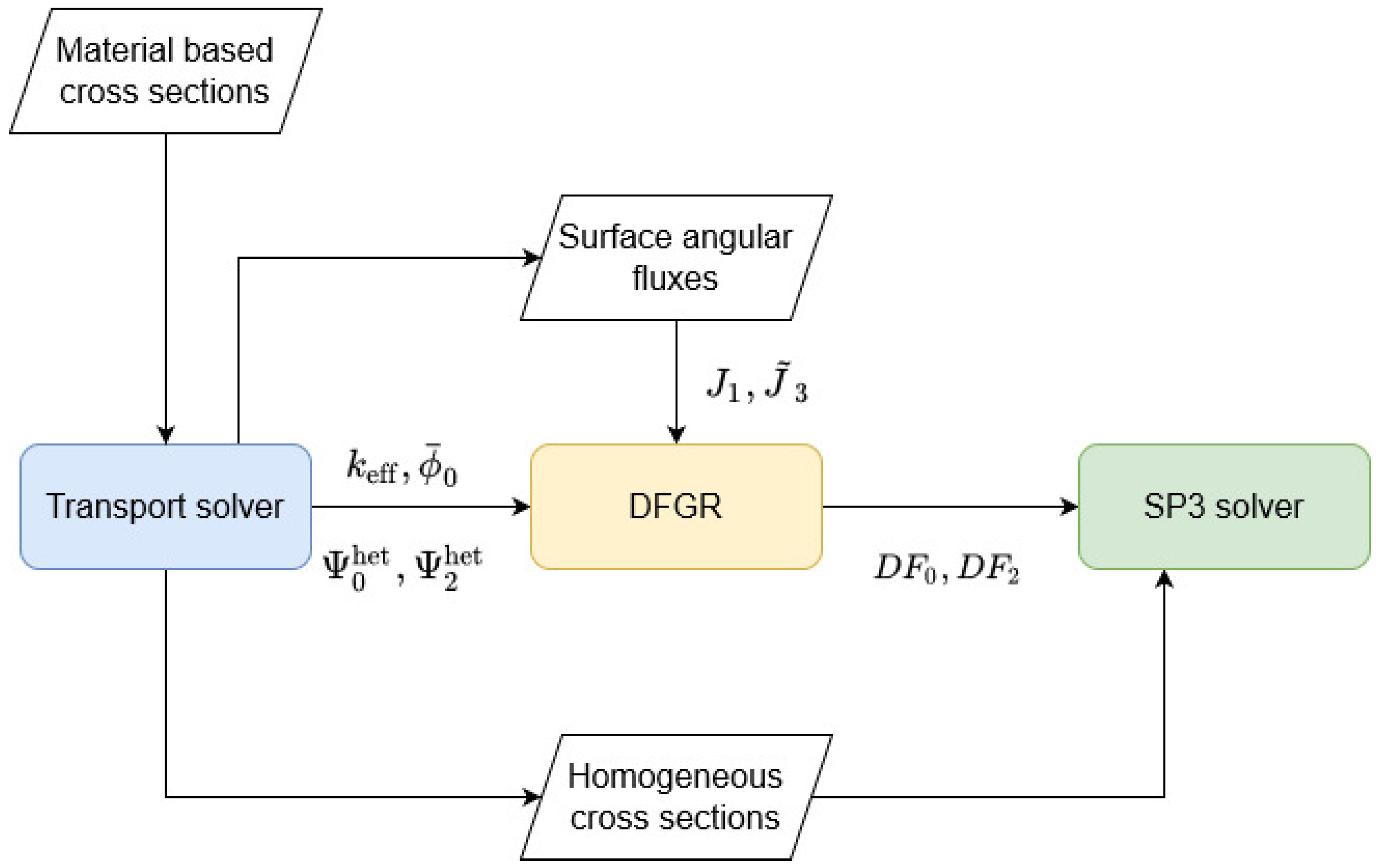
As depicted in Figure 1, the equivalent calculation process devised for the SP₃ solver can be carried out in the following steps:

• Perform the transport calculations and generate quantities including $k_{\mathrm{eff}}$, cell homogenized cross sections, cell averaged scalar flux, and side-dependent surface fluxes and currents.
• Solve the fixed interface problem for each cell sequentially by taking the reference values obtained in step one, generate the SP₃ surface fluxes and currents, then compute the DFs according to their definitions.
• Execute a normal SP3 calculation on a pin-by-pin level using the homogenized cross sections from step one and DFs from step two to obtain the SP₃ solution.

4.2. Practical Approach to Generate SP₃ Discontinuity Factors

The equivalent calculation procedure presented above relies on the whole-core transport solutions, which is not practical in routine calculations and, in a way, defeats the purpose of using low order solvers such as SP₃. Therefore, efforts are also made to explore the feasibility of colorset lattice models to generate equivalent parameters for the core simulation. The three colorset models under consideration are as follows:

• Single-pin model: cross sections are homogenized over the pin cell and DFs are calculated for each of the four surfaces of a pin cell.
• Double-pin model: two pin cells of different type (i.e., material) are placed next to each other and DFs are calculated for each of the four surfaces in each pin cell. The cross sections are taken from the first model.
• Assembly model: both homogenized cross sections and DFs are location dependent, i.e., they are generated for each of the pin cells.

The reflective boundary condition is applied to all three models. Among the three models, the first one is the simplest one and does not capture the leakage between different fuel pins and, thus, is expected to result in a worse performance. The second one captures the effect from neighboring effects to a certain extend but the total number of models increases significantly with the types of fuel pin. The last model supports location-dependent pin-wise homogenizations and DF generation in an environment that is similar to that in the core.

5. Verification of Transported Corrected SP₃ Solver

The newly developed transported corrected SP₃ solver and the corresponding equivalent calculation scheme are verified using the C5G7 benchmark [22]. It is a miniature light water reactor (LWR) with sixteen fuel assemblies (mini core): eight uranium oxide (UO₂) assemblies and eight mixed oxide (MOX) assemblies, surrounded by a water reflector. It features a quarter-core radial symmetry in the 2D configuration, as shown in Figure 2. On the fuel pin level, there are one UO₂ pin, three MOX pins, one guide tube, and one fission chamber. The three MOX fuels pins are 4.3, 7.0, and 8.7% plutonium weight enriched.

In this study, only the core geometry is adopted, and a new set of cross sections is generated in a seven-group energy structure because the original cross sections prepared by the benchmark do not satisfy the unique requirement of the SP₃ solver [15].

The transport code OpenMOC [23] is selected to perform the reference transport calculation because of the convenience of the code to extract node interfaces angular fluxes for DFs generations. However, because the current version only accepts isotropic scattering cross sections, transport corrections are applied to modify isotropic scattering cross sections. All the transport calculations shown below are conducted using the long characteristic method with 32 azimuthal angles, 3 polar angles, the ray trace width of 0.03 cm, and the eigenvalue convergence criterion of $1\times {10}^{-7}$.

5.1. Transport-Corrected SP₃ Method

First, we compare the performance of the base- and transport-corrected SP₃ solver without applying DFs to reveal the impact of the updated interface and boundary conditions. Three cases are selected from the C5G7 benchmark for this purpose, including the UO₂ assembly, MOX assembly, and C5G7 core. In the single assembly cases, pin-wise cross sections are generated using the assembly model with the infinite lattice approximation. For the last case, they are prepared in a whole-core transport calculation, including the cross sections of the water reflector.

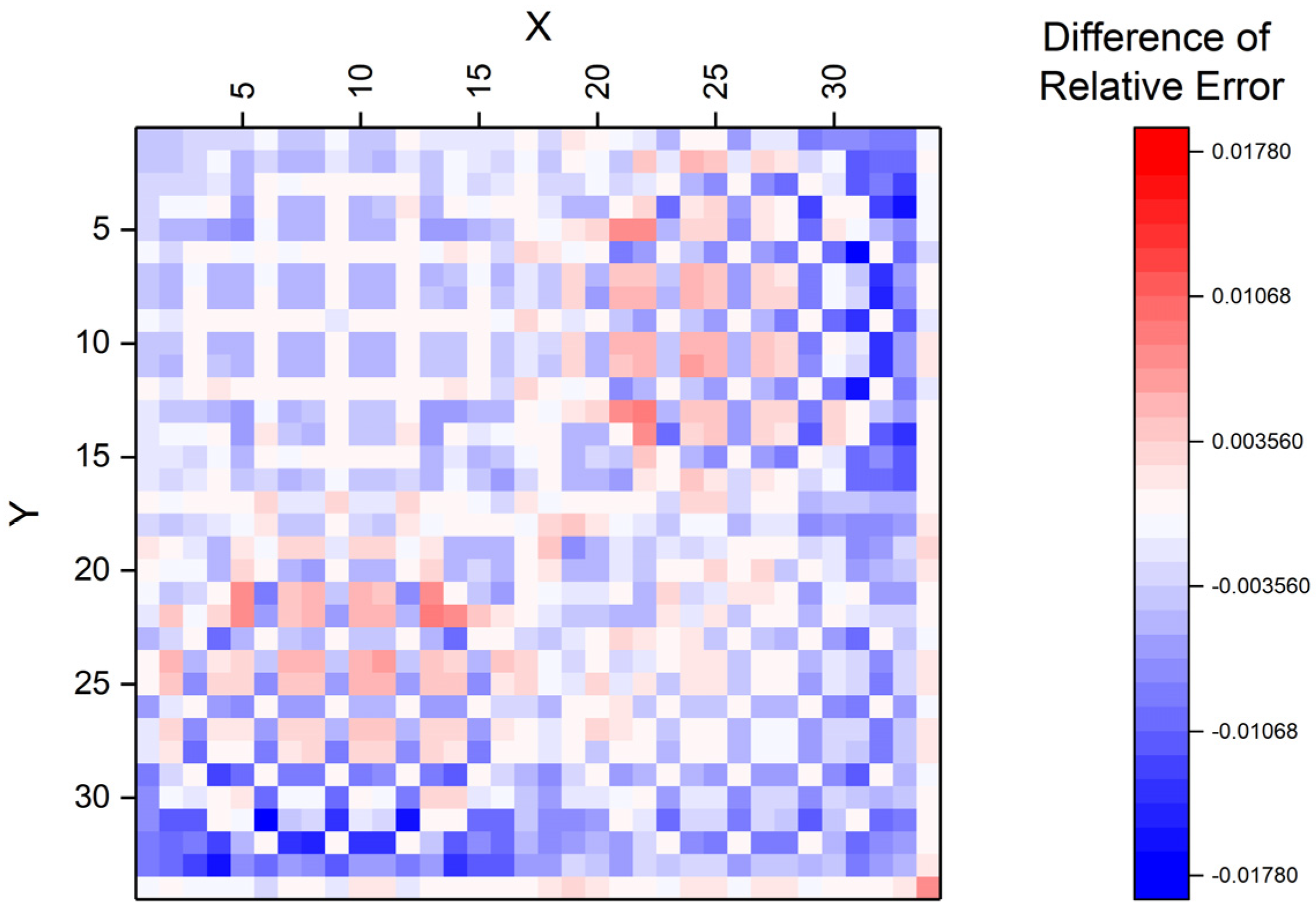
The comparison of the eigenvalue yields negligible differences (less than 10 pcm in all cases), which indicates the correction term $\delta$ in Equation (37) is small and, thus, has a trivial impact on integral parameters such as $k_{\mathrm{eff}}$. The focus has been shifted to local quantities. The absolute relative error in the pin power at all locations is first computed for both solvers as $d=\left|p_{\mathrm{SP}3}/p_{\mathrm{MOC}}-1\right|$, where p denotes the normalized pin power. Then, the difference between the two solvers is calculated as $\Delta =d_t-d_b$, where the subscript t means “transport corrected” and b refers to “base”. The value of $\Delta$ is plotted for the C5G7 core problem according to the pin location, as shown in Figure 3.

The blue regions in the distribution indicate the improved prediction accuracy due to the correction to the interface and boundary conditions. It can be seen that the transport-corrected SP₃ solver yields slightly better pin power distributions, especially at the center of the UO₂ assembly (upper left assembly), regions close to the water reflector (right and bottom surfaces), as well as pin cells next to the fission chamber and guide tubes. As expected, the transport-corrected solver cannot eliminate the prediction error because the spatial homogenization errors still exist.

5.2. Test and Comparison of DFs

Next, the performance of DFs is tested and analyzed in full equivalent calculations. In addition to the three cases used in the previous sub-section, a C5 core problem is also introduced. It contains only fuel assemblies with reflective boundary conditions applied to the outer surface of the geometry. This case would help reveal the impact of DFs on the assembly interfaces by eliminating the effects of the reflector. Following the reference transport calculation, the procedure depicted in Figure 1 is carried out to generate equivalent parameters, inducing the pin-wise cross sections and side-dependent DFs. The equivalent parameters are generated for and applied to each case independently.

It is worth mentioning that numerical instability emerges in regions experiencing a high flux gradient after applying DFs to the NEM response matrix, which forces the spatial discretization to be further refined to achieve convergence. As a result, each pin cell is subdivided into four nodes in equal size and the DFs are only imposed on the outer surface of the pin cell. The refinement allows the flux gradient to occur inside the pin cell; however, the flux is assumed to be constant across surfaces within each pin cell when the DFs are generated. This inconsistency will inevitably introduce errors to the SP₃ calculation.

Table 1. Performance of the transport-corrected NEM SP₃ solver on various benchmark problems. The deviation from the reference results is given in pcm for the eigenvalue and RMS error for the pin power distribution.

Test Case	Solver	Δkeff (pcm)	RMS Error of Pin Power
UO2 assembly	NEM SP3	−125	0.010
	NEM SP3 w/DFs	−5	0.004
MOX assembly	NEM SP3	−38	0.008
	NEM SP3 w/DFs	10	0.001
C5 core	NEM SP3	−171	0.048
	NEM SP3 w/DFs	−75	0.023
C5G7 core	NEM SP3	269	0.049
	NEM SP3 w/DFs	−59	0.023

compares the performance of the transport-corrected SP₃ solver in terms of its prediction of eigenvalue and pin power distribution. It can be seen that the DFs of the GET help reduce the prediction error significantly in all four test cases. The largest improvement is observed in the C5G7 core case, where the deviation from the reference value is reduced by ~200 pcm in eigenvalue and over halved in the root-mean-square (RMS) error of pin power distribution. The prediction accuracy is also drastically improved in the MOX assembly case where the local flux gradient is more profound than that in the UO₂ assembly.

In principle, if the equivalent calculation is conducted properly, the low order operator should reproduce the transport solutions. The non-zero deviations from the reference solution, as shown in Table 1, indicate that the inconsistency between the DF generation and application introduced by the refined 2 × 2 meshing prevent the full equivalent calculation from being performed. Another source of deviation in the last test case stems from the fact that DFs for the nodes in the water reflector are all assumed to be one due to the limitation of the DFGR program. It would tilde the flux distribution in regions across the core/reflector boundary.

Next, various colorset models are tested for their capability to facilitate practical equivalent calculations, because generating equivalent parameters from the whole-core transport solution defeats the purpose of homogenization. The three colorset models described previously are as follows:

• Single-pin model: There are seven models each corresponding to one type of pins. The non-fissionable node, such as guide tubes and water reflector cells, is placed in the center of a 3 × 3 configuration surrounded by UO₂ fuel pins.
• Double-pin model: Eight sets of 2 × 1 pin colorset models are developed for different combination of pin cells. These DFs will be used in the whole core on the interface between neighboring different cells.
• Assembly model: Single UO₂ and MOX assembly models.

A fourth model is also considered, which is a mix of options two and three. The DFs from the assembly colorset are used on node interfaces inside an assembly, while those from the double-pin colorset are used on the assembly interfaces. The comparison of the results of the C5G7 core calculation is listed in

Table 2. Performance of the transport-corrected SP₃ solver using different DF generation models. The deviation from the reference results is given in pcm for the eigenvalue and RMS error for the pin power distribution.

Colorset Model	Δkeff (pcm)	RMS Error of Pin Power
Single pin	273	0.056
Double pin	336	0.056
Assembly	288	0.048
Assembly + double pin	272	0.047

.

We observe that the calculation accuracy in terms of the eigenvalue and pin power distribution is improved slightly and consistently as the size of the colorset model increases. The assembly model shows improved results compared to the single-pin and double-pin models and the addition of DFs on the assembly interfaces from the double-pin model (option four) further reduces the prediction error.

It is expected that the use of DFs from the single-pin and double-pin models would not yield noticeably improved solutions, if any, compared with the results obtained without DFs, because DFs and associated cross sections are only applicable for the environment (spectrum and boundary conditions) within which they are generated. However, it is somewhat unexpected that none of the colorset models significantly outperform the approach without DFs in Table 1. That is to use only the location-dependent cross sections generated from the whole-core reference transport solution, although the associated computational cost in the latter case would be massively elevated. Figure 4 shows the relative error of the predicted pin power in the C5G7 whole-core calculation using the cross sections and DFs generated in option three. It can be seen that the main discrepancies occur in regions near the interface between the active core and reflector, where the SP₃ solution largely underestimates the fission power and neutron flux, while a uniform overestimation is observed in the central UO₂ assembly. An almost identical trend is also found in the comparison of the SP3 solution with option four against the transport results, which is expected because the DFs for nodes along the core/reflector interface are missing in both options three and four.

The results above imply that the impact of two factors in the equivalent calculation, the homogenized cross sections, and DFs, almost contribute equally to the prediction accuracy with regard to the eigenvalue and power distribution. The largest impact is found in regions in the vicinity of material boundaries, especially the core boundary, suggesting that colorset models including non-multiplying regions must be properly developed and tested. Effort should also be made in the future to determine the optimal approach to perform equivalent calculations for the SP₃ solver.

6. Conclusions and Outlook

In this work, we focus on the development of a transport-corrected nodal SP₃ solver for the equivalent reactor core calculation. The response matrix in the NEM SP₃ solver has been reformulated based on the recently published new SP₃ theory with rigorously derived interface and boundary conditions, while the computation scheme in the NEM is kept intact. A streamlined process of generating DFs of the GET for the correction of pin-by-pin homogenization error has been implemented, which incorporates the high-fidelity transport code and an in-house developed DF generation program. We also propose a few models with varying sizes for the generation of equivalent parameters aiming to further reduce the computational burden and explore their feasibility to practical applications. The transport-corrected SP₃ solver and various colorset models are tested on the mini-core C5G7 benchmark problem.

It was found that the transport-corrected SP₃ solver can compute the inter-node leakage rate correctly due to the updated interface and boundary conditions and, thus, improve the prediction of the pin power distribution. In the whole-core calculation, the regions benefiting the largest improvement are located at the center of the core, close to the water reflector, and next to the fission chamber and guide tubes.

The performance of DFs is tested and analyzed in full equivalent calculations. We can see that the DFs of the GET can reduce the prediction error significantly in all the test cases from the single assembly, active core, and core with reflectors. In the last case, the deviation from the reference transport solutions is reduced by ~200 pcm in eigenvalue and over halved in the RMS error of pin power distribution. In order to increase the feasibility of the equivalent calculation scheme to practical applications, a number of colorset models are introduced and analyzed, including the single-pin, double-pin and assembly models. With DFs, the assembly colorset model slightly outperforms the most accurate homogenization approach without DFs while maintaining a superior computational efficiency. However, using DFs from various colorset models fails to achieve the prediction accuracy at the same level of the case when DFs are produced using the whole-core transport solution.

This study has also identified a few discrepancies in the implementation of the transport-corrected SP₃ methodology. For example, it has experienced numerical instabilities that cause an issue to achieve a converged solution when the DFs are imposed. Our preliminary investigation points to the use of the 1D forth order polynomial nodal expansion method implemented in the NEM solution method. We plan to implement and test a semi-analytical nodal expansion method in the future work to resolve this issue.

The inability to generate DFs for the water nodes in the reflectors is also found to be partially responsible for the deviations of the SP₃ results from the reference transport solution. Thus, the DF generation program will be revisited and updated to solve the fixed interface problem for the reflector region. At last, effort will continue to investigate colorset models that can maximize the benefit of the equivalent calculations while maintaining the computational cost to a reasonable level for practical whole-core simulations.

References

Gelbard, E.M. Application of Spherical Harmonics Method to Reactor Problems; Bettis Atomic Power Laboratory: West Mifflin, PA, USA, 1960; Technical Report No. WAPD-BT-20.
Pomraning, G. Asymptotic and variational derivations of the simplified PN equations. Ann. Nucl. Energy1993, 20, 623–637. [Google Scholar] [CrossRef]
Larsen, E.W.; Morel, J.E.; McGhee, J.M. Asymptotic Derivation of the Multigroup P1 and Simplified PN Equations with Anisotropic Scattering. Nucl. Sci. Eng.1996, 123, 328–342. [Google Scholar] [CrossRef]
Litskevich, D.; Merk, B. SP3 solution versus diffusion solution in pin-by-pin calculations and conclusions concerning advanced methods. J. Comput. Theor. Transp.2014, 43, 214–239. [Google Scholar] [CrossRef]
Kozlowski, T.; Xu, Y.; Downar, T.J.; Lee, D. Cell homogenization method for pin-by-pin neutron transport calculations. Nucl. Sci. Eng.2011, 169, 1–18. [Google Scholar]
Yu, L.; Lu, D.; Chao, Y.A. The calculation method for SP3 discontinuity factor and its application. Ann. Nucl. Energy2014, 69, 14–24. [Google Scholar] [CrossRef]
Cabellos, O.; Aragones, J.M.; Ahnert, C. Generalized Effects in Two Group Cross Sections and Discontinuity Factors in the DELFOS Code for PWR Cores. In Proceedings of the M&C’99 International Conference on Mathematics and Computation, Reactor Physics and Environmental Analysis in Nuclear Applications, Madrid, Spain, 27–30 September 1999; pp. 700–709. [Google Scholar]
Park, K.W.; Park, C.J.; Lee, K.T.; Cho, N.Z.; Kim, Y.H. Pin-Cell Homogenization via Generalized Equivalence Theory and Embedding Assembly Calculation. Trans. Am. Nucl. Soc.2001, 85, 334–336. [Google Scholar]
Kozlowski, T.; Lee, D.; Downar, T.J. The Use of An Artificial Neural Network for On-line Prediction of Pin-Cell Discontinuity Factors in PARCS. In Proceedings of the PHYSOR 2004, Chicago, IL, USA, 25–29 April 2004. [Google Scholar]
Yamamoto, A.; Sakamoto, T.; Endo, T. Discontinuity factors for simplified P3 theory. Nucl. Sci. Eng.2016, 183, 39–51. [Google Scholar] [CrossRef]
Chiba, G.; Tsuji, M.; Sugiyama, K.I.; Narabayashi, T. A note on application of superhomogénéisation factors to integro-differential neutron transport equations. J. Nucl. Sci. Technol.2012, 49, 272–280. [Google Scholar] [CrossRef] [Green Version]
Thompson, S.A.; Ivanov, K.N. Advances in the Pennsylvania State University NEM code. Ann. Nucl. Energy2016, 94, 251–262. [Google Scholar] [CrossRef]
Xu, Y.; Hou, J.; Ivanov, K. Improvement to NEM SP3 Modelling and Simulation. In Proceedings of the PHYSOR 2020, Cambridge, UK, 29 March–2 April 2020. [Google Scholar]
Xu, Y.; Hou, J.; Ivanov, K. Implementation of Second-Order Discontinuity Factor for Simplified P3 Theory in NEM. In Proceedings of the PHYSOR 2018: Reactors Physics Paving the Way towards More Efficient Systems, Cancun, Mexico, 21–26 April 2018. [Google Scholar]
Chao, Y.A. A new and rigorous SPN theory for piecewise homogeneous regions. Ann. Nucl. Energy2016, 96, 112–125. [Google Scholar] [CrossRef]
Chao, Y.A. A new and rigorous SPN theory–Part II: Generalization to GSPN. Ann. Nucl. Energy2017, 110, 1176–1196. [Google Scholar] [CrossRef]
Xu, Y. Generalized Equivalent nodal SP3 Methodology for Reactor Simulations. Ph.D. Thesis, North Carolina State University, Raleigh, NC, USA, 2020. [Google Scholar]
Smith, K. Assembly homogenization techniques for light water reactor analysis. Prog. Nucl. Energy1986, 17, 303–335. [Google Scholar] [CrossRef]
Koebke, K. A New Approach to Homogenization and Group Condensation; International Atomic Energy Agency: Vienna, Austria, 1980; No. IAEA-TECDOC-231. [Google Scholar]
Chao, Y.A.; Yamamoto, A. The explicit representation for the angular flux solution in the simplified PN (SPN) theory. In Proceedings of the PHYSOR 2012: Advances in Reactor Physics Linking Research, Industry and Education, Knoxville, TN, USA, 15–20 April 2012. [Google Scholar]
Lewis, E.E.; Smith, M.A.; Tsoulfanidis, N.; Palmiotti, G.; Taiwo, T.A.; Blomquist, R.N. Benchmark Specification for Deterministic 2-D/3-D MOX Fuel Assembly Transport Calculations without Spatial Homogenization; Organisation for Economic Co-operation and Development: Paris, France, 2001; (C5G7 MOX). NEA/NSC 280. [Google Scholar]
Boyd, W. The OpenMOC Method of Characteristics Neutral Particle Transport Code. Ann. Nucl. Energy2014, 68, 43–52. [Google Scholar] [CrossRef] [Green Version]
Figure 1.
Procedure of equivalent core calculation using SP3 solver.
Figure 2.
OpenMOC model for C5G7 core. Materials are distinguished by different colors.
Figure 3.
Differences in relative pin power using the base and transport-corrected SP3 solvers. Blue regions indicate improved predictions by the transport-corrected SP3 solver, while red regions mean the opposite.
Figure 4.
Relative differences in pin power distribution predicted by a transport-corrected SP3 solver from the reference transport solution. The cross sections and DFs are generated using the assembly model (option 3).