Hybrid PV Power Forecasting Methods: A Comparison of Different Approaches

Abstract

Accurate photovoltaic (PV) prediction has a very positive effect on many problems that power grids can face when there is a high penetration of variable energy sources. This problem can be addressed with computational intelligence algorithms such as neural networks and Evolutionary Optimization. The purpose of this article is to analyze three different hybridizations between physical models and artificial neural networks: the first hybridization combines neural networks with the output of the five-parameter physical model of a photovoltaic module in which the parameters are obtained from a datasheet. In the second hybridization, the parameters are obtained from a matching procedure with historical data exploiting Social Network Optimization. Finally, the third hybridization is PHANN, in which clear sky irradiation is used as an input. These three hybrid methods are compared with two physical approaches and simple neural network-based forecasting. The results show that the hybridization is very effective for achieving good forecasting results, while the performance of the three hybrid methods is comparable.

1. Introduction

In the last 20 years, the penetration of renewable energy sources (RESs) in energy systems around the world has progressively increased due to the rise of environmental concerns and governmental policies. Of the different RESs, the worldwide growth of photovoltaic (PV) technologies has been close to exponential [1].

The most important and challenging problem arising from the great penetration of PV in electrical systems is the high level of variability in the power supplied. In fact, this strictly depends on local weather conditions, such as cloud cover, temperature, wind speed and atmospheric aerosol levels. The resulting uncertainty and variability of the PV power profile create various problems for the management of the electricity grid. First, large frequency oscillations can be induced by abrupt changes in power; secondly, in the case of the high penetration of renewables, reverse active power flows may occur in the medium-voltage distribution power supply, or even in the high-voltage transmission line. Finally, the high penetration of PV increases the costs of the allocation of the spinning reserve, ancillary services and the energy planning of the dispatchable generators [2].

For all these reasons, highly accurate photovoltaic power prediction systems are required to optimize the management of the electricity grid from both a technical and economic point of view, without reducing energy reliability and quality.

Computational intelligence (CI) techniques, such as Artificial Neural Networks (ANN) and Evolutionary Algorithms (EAs), have become very popular approaches to problems such as the modeling of non-linear systems, parameter identification, design and control optimization of electric systems and long-term to short-term forecasting.

In [3], the authors exploit a well-known Evolutionary Algorithm, namely the Firefly Algorithm (FA), for the optimal sizing of stand-alone photovoltaic systems. System component selection is performed regarding not only the PV modules and the inverters but also the batteries and the charge controller. A key point resulting from this study is the scalability and the flexibility of the proposed methodology.

The optimal sizing of PV systems can also be analyzed considering several performance parameters. In [4], the authors exploit a multi-objective Differential Evolution to face technical and economic criteria at the same time when sizing stand-alone or grid-connected PV systems. Computational intelligence algorithms can be used also in the loss prediction forecasting of PV plants under peculiar conditions. In [5], the authors developed and tested a three-stage model based on computational intelligence techniques for predicting the snow losses in PV production. Different models were tested in the paper, such as Random Forests, Regression Trees and Artificial Neural Networks, with the latter showing the best performance.

In the design stage of PV plants, CI algorithms can be used to find the optimal tilt angle and orientation. This problem has been solved in [6] with the Harmony Search algorithm analyzing different climate scenarios, and the proposed technique has been further investigated in [7] in the context of zero-energy buildings.

In [8], the Ant Colony Optimization algorithm was used to build an Maximum Power Point Tracking (MPPT) controller to manage partial shadows on PV modules in a globally optimal way. A similar problem has been approached in [9] with Particle Swarm Optimization (PSO) and in [10] with a hybrid PSO–ANN method. In [11], an Improved Particle Swarm Optimization method was used in the MPPT problem for PV modules with partial shadows to overcome some of the traditional issues that PSO shows in this problem [12]. An alternative approach for MPPT identification under partial shadows is the use of Random Forest [13].

Photovoltaic module parameter extraction is another problem that is often solved by CI techniques. In [14], the authors propose an efficient and fast method for the online parameter identification of the photovoltaic single-diode model, combining Genetic Algorithms and explicit equations. In [15], the Symbiotic Organisms Search algorithm was used to solve the PV model parameter identification problem. This algorithm was compared with many other state-of-the-art Evolutionary Algorithms, such as Biogeography-based Learning Particle Swarm Optimization, the Across Neighborhood Search, the Chaotic Teaching-Learning Algorithm, the Competitive Swarm Optimizer and the Levy Flight trajectory-based Whale Optimization Algorithm. In [16], the results of the model parameter identification with Social Network Optimization were analyzed to identify the main criticalities. Finally, in [17], the comparison between Evolutionary Algorithms was extended to the case of a double diode model and a complete photovoltaic module model.

Power production forecasting is another important problem that is often tackled with computational intelligence techniques. In [18], a decision making process for identifying the most effective training parameters and structural characteristics was proposed for the specific case of a physical hybrid method (PHANN). In [19], different training approaches were compared for PHANN, introducing the ensemble method and new performance indexes such as the envelope-weighted mean absolute error. Finally, in [20], PHANN was compared with a physical model trained with social network optimization.

Finally, a new trend in PV power forecast is nowcasting; i.e., short-term forecasting. In this field, in [21], hybrid fuzzy clustering was tested for nowcasting; in [22], CI techniques were exploited to perform nowcasting from radar information, and in [23], neural networks were used as a robust and accurate method for sun identification in all-sky images.

The purpose of this paper is to analyze the impact on the forecasting accuracy of different hybridizations between physical models and artificial neural networks. The first hybridization approach combines neural networks with the output of the five-parameter physical model of a photovoltaic module: the parameters of this model are obtained from the datasheet information. In the second hybridization approach, these parameters are obtained from a matching procedure with historical data exploiting an Evolutionary Algorithm, namely Social Network Optimization. Finally, the third hybridization method is PHANN, in which clear sky irradiation is used as the input for of the neural network.

The structure of the paper is the following: in Section 2, the physical and hybrid models are analyzed. In Section 2.1, both the physical model and the two possible matching procedures are analyzed, while in Section 2.2, the PHANN model is briefly introduced and the new system, called P5ANN, is described. The results of the proposed methods are shown in Section 3: at the beginning of this section, the results obtained by the two physical models are presented and discussed, and then the comparison between the two proposed P5ANN and PHANN methods is presented and their specific features are analyzed. Finally, some conclusions are reported in Section 4.

2. Methods

In this section, the methods analyzed in this paper are presented. In particular, Section 2.1 presents the physical methods and Section 2.2 presents the hybrid methods. The methods here proposed exhibit general valence, even if in Section 3 they have been applied to a specific case study.

2.1. Physical Models

The PV cell equivalent-circuit models are the mathematical tools that represent PV cells’ electrical behavior in terms of an I–V curve and the resulting power–voltage curve (P–V curve). The equivalent-circuit model of a PV device (for example, a module, a string or an integer for a PV field) is obtained starting from the equivalent circuit of the cell by inserting the series and/or parallel relations, which represent the actual connections of the PV cells in the device.

Various equivalent circuits to PV cells are reported in the literature. They differ in their number of elements and in their circuit topology, and consequently in the number of parameters required to characterize them.

Most of the model parameters depend on irradiance and temperature, so they are related to environmental conditions; i.e., the irradiance on the plane of the PV cell G, the so-called plane of array (POA) irradiance and the PV cell temperature $T_C$ resulting from the POA irradiance and the ambient temperature $T_{amb}$.

The simplest equivalent-circuit model for a PV cell consists of a parallel between a real diode and an ideal current source [24]. The accuracy of this model can be increased by adding the series resistance $R_S$, which mainly represents the resistance at the semiconductor interface, and the shunt resistance $R_{SH}$, which models high-current paths through the semiconductor along material dislocations and mechanical defects [24]. A further increase in model accuracy is achieved by adding a second diode to the circuit model of the PV cell, leading to the double-diode model [25]. The trade-off between accuracy, equivalent-circuit complexity, parameter calculation and computational burden usually leads to the so-called five-parameter model being preferred, which is the single-diode model including both $R_S$ and $R_{SH}$ parasitic resistors. In this work, the single diode five-parameter model is selected to represent the PV module. The equivalent circuit is shown in Figure 1.

2.1.1. Maximum Power Point Calculation

Starting from the PV generator’s I–V curve, it is possible to compute the maximum power output. In mathematical terms, the output of the PV generator is the function (f): the inputs are the equivalent-circuit model parameters, ($\underline{p}$), which in turn depend on the environmental data ($\underline{w}$). Consequently, the power at the maximum power point, $P_{MPP}$ can be written as

$$P_{MPP}=f\left(\underline{p}\left(\underline{w}\right)\right)$$

(1)

The procedure for selecting the correct set of parameters in reference to a specific environmental condition $\underline{p}$ is called matching. Usually, standard test conditions ($STC$, defined as solar irradiation $G_{STC}$ = 1000 W/m², a cell temperature $T_{C,STC}$ of 25 °C and an air mass of 1.5 and indicated by the vector ${\underline{w}}_{STC}$) are taken into account to define the set of reference parameters, indicated by the vector ${\underline{p}}_{STC}$.

Different matching procedures have been presented in the literature: they are based on the matching of rated values reported in the datasheet or on the matching with some measurements. In this paper, two methods belonging to both matching procedures, respectively, are considered.

The first method matches the set of reference parameters in order to comply with the reference data reported in the datasheet of the PV module [26,27,28]; then, irradiance and temperature corrections are applied to calculate the set of parameters which represent the actual environmental conditions. Some drawbacks affect this method, such as numerical instability or convergence on unfeasible solutions; i.e., a negative value for a series resistor.

The second method selects the parameters in order to fit the real data of a PV generator. This approach requires a large number of tests, in which the environmental conditions and the PV generator output power should be accurately measured. A proper redundancy in the dataset could make the process robust with respect to some errors in the measurements. Moreover, computational problems are reduced.

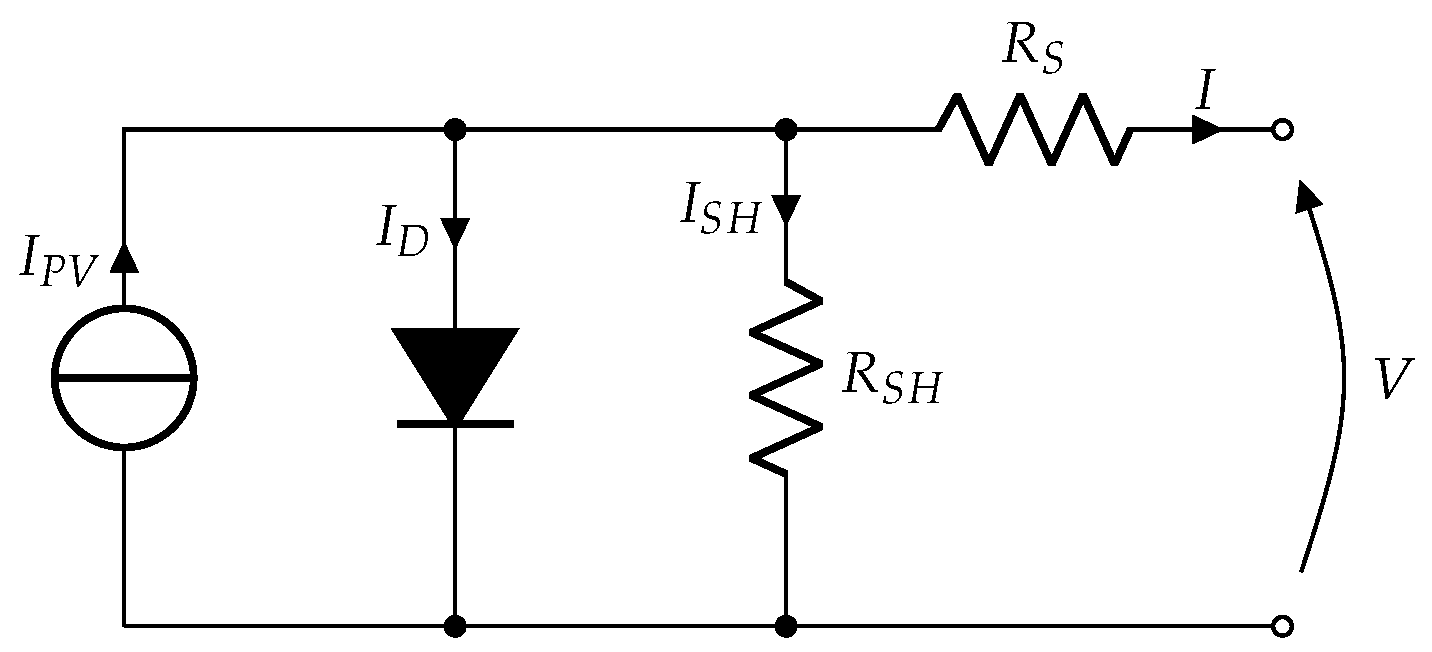
2.1.2. Five-Parameter PV Model

The PV cell I–V curve is derived from the solution of the five-parameter equivalent circuit model: the constitutive relation of Kirchhoff’s laws and elements leads to the following equation [27]:

$$I(G,T_C)=I_{PV}(G,T_C)-I_0\left(T_C\right)·\left(e^{\frac{V+R_{S}I}{a}-1}\right)-{\displaystyle \frac{V+R_{S}I}{R_{SH}\left(G\right)}}$$

(2)

where $R_S$ and $R_{SH}$ are, respectively, the series and shunt resistances, $I_{PV}$ is the photogenerated current, $I_0$ is the diode reverse saturation current and a is the ideality factor parameter.

The ideality factor depends on the PN junction ideality factor (n), on the absolute temperature of the PN junction ($T_C$), on the Boltzmann constant ($k=1.380649·{10}^{23}J/K$) and on the electron charge magnitude ($q=1.602176634·{10}^{-19}C$):

$$a=\frac{n·k·T_C}{q}$$

(3)

The series resistance $R_S$ makes the equation implicit: the I–V curve can be easily calculated in a numerical manner, while the closed-form solution is based on the Lambert W-function [29].

The junction temperature depends on the POA irradiance on the cell, ambient temperature, wind speed and direction. The actual cell temperature can be measured by means of a resistance temperature detector (RTD) on the back of the PV module [30]; otherwise, it can be evaluated from thermal models [31].

The easiest and the most widely used thermal model in PV modules is based on the normal operating cell temperature ($NOCT$), which assumes the difference between the cell and ambient temperature ($T_{amb}$) to be proportional to the POA irradiation. Thus, the PV cell temperature can be computed as

$$T_C=T_{amb}+\frac{NOCT-T_{amb@NOCT}}{G_{NOCT}}·G;$$

(4)

where the ambient temperature and the POA irradiance in these conditions are $T_{amb@NOCT}$ = 20 °C and $G_{NOCT}$ = 800 W/m². The wind speed is assumed to be 1 m/s and without thermal convection on the back of the PV module. The photogenerated current is irradiance and temperature-dependent:

$$I_{PV}(G,T_C)=\frac{G}{G_{STC}}·\left[I_{PV,STC}·\left(1-{\alpha }_{ISC}(T_C-T_{C,STC})\right)\right]$$

(5)

where $I_{PV,STC}$ is the reference photogenerated current at STC, and ${\alpha }_{ISC}$ is the short-circuit current temperature coefficient.

The reverse bias saturation current is temperature-dependent:

$$I_0\left(T_C\right)=I_{0,STC}·{\left(\frac{T_C}{T_{STC}}\right)}^3·e^{\frac{E_g\left(T_{C,STC}\right)}{n·k·T_{STC}}-\frac{E_g\left(T_C\right)}{n·k·T_C}}$$

(6)

where k is the Boltzmann constant and $E_g$ is the bandgap energy of the silicon, which in turn is temperature-dependent:

$$E_g\left(T\right)=1.17-4.73·{10}^{-4}·\frac{T^2}{T+636};$$

(7)

Finally, the irradiance correction of the shunt resistance is

$$R_{SH}=R_{SH,STC}·\frac{G_{STC}}{G}$$

(8)

It is assumed that the ideality factor n and series resistance $R_S$ are independent of temperature and irradiation [27,28].

2.1.3. Parameter Identification from Datasheet

The matching procedure based on data reported in the datasheet and applied to the five-parameter equivalent circuit model allows the identification of the set of parameters, which are $I_{PV}$, $I_0$, n, $R_S$ and $R_{SH}$, which is referred to as the STC, by solving a set of five independent simultaneous equations. Three specific current–voltage pairs belonging to the I–V curve are usually available from the datasheet: the open circuit voltage (0, $V_{OC}$), the short circuit current ($I_{SC}$, 0) and the maximum power point ($I_{MPP}$, $V_{MPP}$). The evaluation of Equation (2) in these points leads to the following subset of three equations:

$$I_{PV}(G_{STC},T_{C,STC})-I_0\left(T_{C,STC}\right)·\left(e^{\frac{V_{OC}}{a}-1}\right)-{\displaystyle \frac{V}{R_{SH}\left(G_{STC}\right)}}=0$$

(9)

$$I_{PV}(G_{STC},T_{C,STC})-I_{SC}-I_0\left(T_{C,STC}\right)·\left(e^{\frac{R_S{I}_{SC}}{a}-1}\right)-{\displaystyle \frac{R_S{I}_{SC}}{R_{SH}\left(G_{STC}\right)}}=0$$

(10)

$$I_{PV}(G_{STC},T_{C,STC})-I_{MPP}-I_0\left(T_{C,STC}\right)·\left(e^{\frac{V_{MPP}+R_S{I}_{MPP}}{a}-1}\right)-{\displaystyle \frac{V_{MPP}+R_S{I}_{MPP}}{R_{SH}\left(G_{STC}\right)}}=0$$

(11)

Two more equations are necessary to calculate the reference parameters. These additional constraints have to be chosen according to the expected properties of the I–V and P–V curves. First of all, the derivative of the P–V curve at maximum power point has to equal zero, leading to the following equation:

$$I_{MPP}-V_{MPP}{\displaystyle \frac{{\displaystyle \frac{I_0\left(T_{C,STC}\right)}{a}}{e}^{\frac{V_{MPP}+R_S{I}_{MPP}}{a}}+{\displaystyle \frac{1}{R_{SH}}}}{1+{\displaystyle \frac{I_0\left(T_{C,STC}\right)R_S}{a}}{e}^{\frac{V_{MPP}+R_S{I}_{MPP}}{a}}+{\displaystyle \frac{R_S}{R_{SH}}}}}=0$$

(12)

There are different constraints which can be considered to choose the last equation: they can be the slope of the I–V curve at the short circuit point [32] or the slope of the I–V curve at the open voltage point [33]. The derivatives of the current with the voltage under short-circuit and open-voltage conditions are mainly determined by the shunt resistance $R_{SH}$ and the series resistance $R_S$, respectively:

$${\left.\frac{dI}{dV}\right|}_{\begin{array}{l}V=0\\ I=I_{SC}\end{array}}\simeq -\frac{1}{R_{SH}}$$

(13)

$${\left.\frac{dI}{dV}\right|}_{\begin{array}{l}V=V_{OC}\\ I=0\end{array}}\simeq -\frac{1}{R_S}$$

(14)

Besides the slope of the I–V curve at specific points, the open circuit voltage or the short circuit current at a cell temperature different from STC [26] can be considered; knowledge of the open circuit voltage and short circuit current temperature coefficients is necessary.

In this work, the derivative of the current with the voltage evaluated at the short circuit current was chosen to complete the set of equations [32], resulting in

$$\frac{1+{\displaystyle \frac{I_0\left(T_{C,SRC}\right)R_S}{a}}{e}^{\frac{R_S{I}_{SC}}{a}}+{\displaystyle \frac{R_S}{R_{SH}}}}{{\displaystyle \frac{I_0\left(T_{C,SRC}\right)}{a}}{e}^{\frac{R_S{I}_{SC}}{a}}+{\displaystyle \frac{1}{R_{SH}}}}-R_{SH}=0$$

(15)

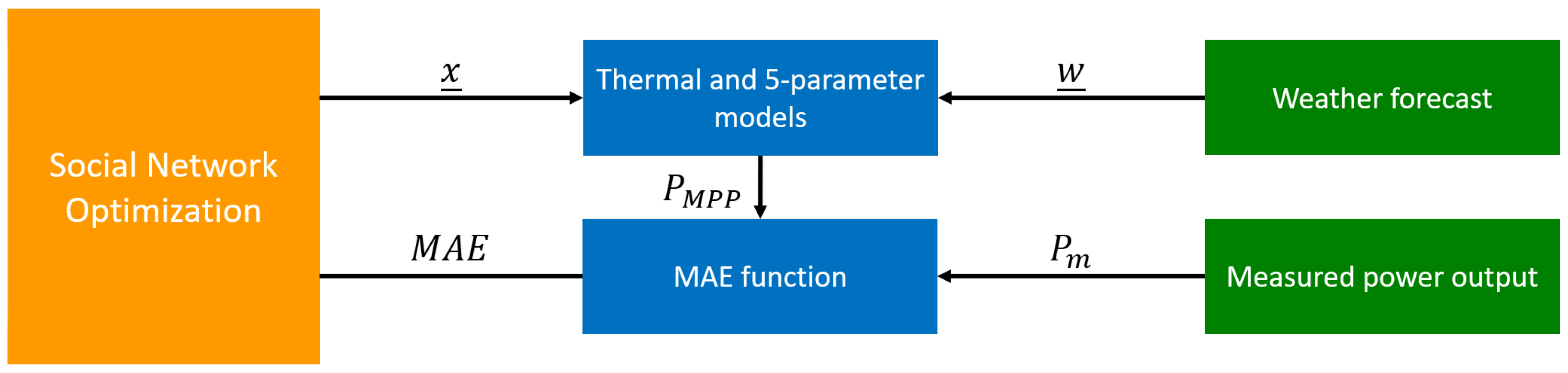
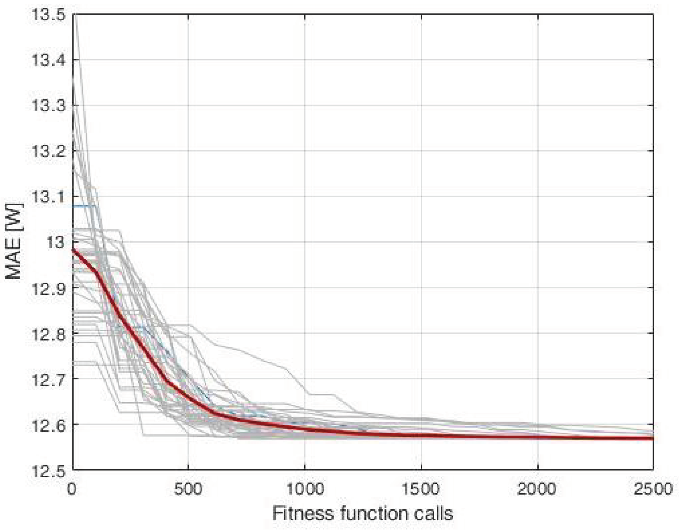
2.1.4. Parameter Identification with EAs

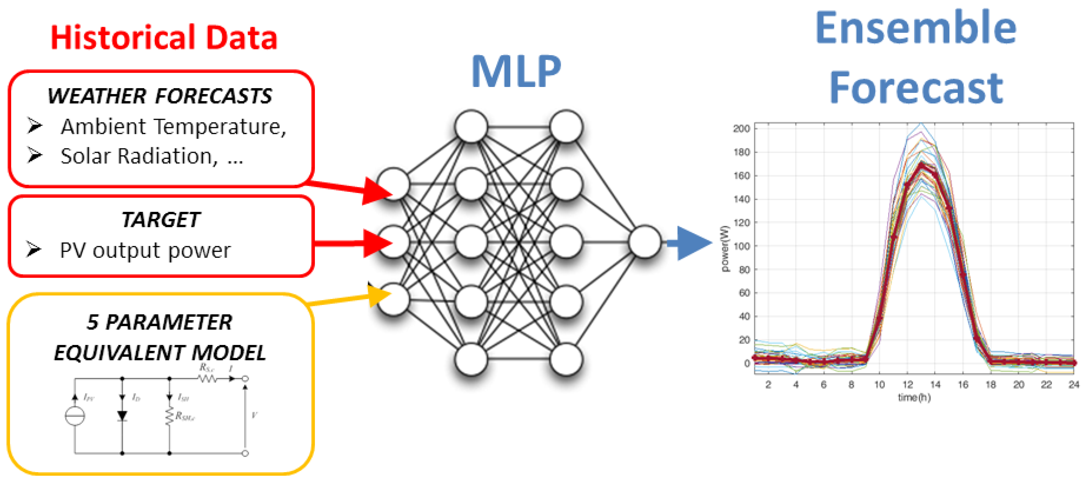
The parameters of the model can be obtained in an alternative way through an optimization process which aims to find the best set of parameters to fit the measurement data.

This procedure can be formulated as a minimization problem in the following way:

$$\underset{\underline{x}\in \mathcal{X}}{min}MAE\left(\underline{x}\right)$$

(16)

where $\underline{x}$ is a vector containing the set of tentative parameters, $\mathcal{X}$ is the search domain for this problem, and $MAE$ is the mean absolute error function between the measured power data ($P_m$) and the output power estimated with the fiv- parameter model ($P_{MPP}$):

$$MAE=\frac{1}{N}\sum _{i=1}^N|P_{m,i}-P_{MPP,i}\left(\underline{x}\right)|$$

(17)

where N is the number of samples in the dataset used in the optimization procedure.

This minimization problem is characterized by many local minima and, therefore, Evolutionary Algorithms (EAs) are suitable for this application. In particular, in this paper, the matching problem was addressed with Social Network Optimization (SNO); this algorithm has already shown good performance on both standard benchmarks and on a large number of different engineering problems [34].

The procedure adopted in this matching problem is depicted in Figure 2. The algorithm creates, by means of its working principles, a candidate solution $\underline{x}$ containing the reference parameters. They are used in the thermal and five-parameter models in combination with the weather forecasts ($\underline{w}$) containing ambient temperature and irradiance. The physical models take as an output the forecasted power $P_{MPP}$, which is compared with the measured one ($P_m$) by means of the $MAE$ error. This is fed-back to SNO and exploited to produce a new population of candidate solutions.

The termination criterion used in this work for SNO is the maximum number of cost function calls: in fact, this parameter is proportional to the total computational time required because the self-time of the optimization algorithm is negligible with respect to the cost function computation. The algorithm population is set to 25 individuals and 100 iterations have been done, and thus 2500 objective function calls are performed.

Figure 3 shows the convergence curves for 40 independent optimization trials on a matching problem with 20 training days. The low dispersion at the end of the optimization of the thin lines (representing each independent trial) around the thick line (average convergence) shows the robustness of the optimization algorithm in this problem.

The number of training days—i.e., the days used in the matching procedure—is an important user-defined parameter. In fact, this tunes the trade-off between the computational time and the final performance. Two aspects should be analyzed: the solution should be robust with respect to the training set selection and the performance on the training set (training performances) should be a good estimation of the performance on a new dataset (testing performances).

In order to analyze the first aspect, the training set size has been changed from 1 day to 260 days, with a denser grid at the beginning. For each training set size, 40 random trials were performed, each with a different selection of days. The results are shown in Figure 4a, where the average value, the first and the third quartiles are reported. Increasing the training set size decreased the standard deviation; a good value for the training set size was found to be above 50 days.

In order to determine the training set size that is also significant for the testing performances, a test very similar to the one proposed above can be used. The result is called a learning curve. In this activity, both the training error, computed on the dataset used in the matching procedure, and the testing error, computed on the entire year of measures, are monitored. Figure 4b shows the learning curves. For each dataset size, 40 independent trials were performed, extracting for each one a different training dataset.

Analyzing the results of Figure 4b, it is possible to see that, with a training set with at least 60 days, the results are quite stable and the training error is a good estimation of the testing set. Combining these results with those shown before, it is possible to say that 60 training days is a good compromise between accuracy and computational time that grows linearly with the increase of the training set size.

2.2. Hybrid Models

Forecasting methods, as previously mentioned, cover a wide variety of approaches and therefore can be classified in different ways according to the emphasized features in the model itself. For these reasons, the same technique might belong to different classes, and moreover, the same forecasting method could fall within the intersection of two existing classes. Thus, there are different forecasting method descriptions and classifications available in the literature, some of which divide models between “direct” or “indirect” methods based on whether the target parameter is directly forecasted. “Model-driven approaches” and “data-driven” approaches—or “physical” and “stochastic” forecasting methods, which actually might be synonyms for the previous—allow a third group of models, namely the “hybrid” group, which shares some features in common with the other previously listed classes. It has been proven that, by gathering the strengths of the original methods, the new generated hybrid models have enhanced forecasting capabilities [20,35]. In this particular application, the comparison is performed by means of a hybrid model which aims at combining the five-parameter equivalent model of the PV module and the stochastic Artificial Neural Network, and therefore our model has been named P5ANN. In more detail, the main objective of this work is to provide a fair comparison of the forecasting capabilities of different methods in combination: ANN with both a physical model of clear sky solar radiation (PHANN) and the electrical equivalent model of the PV module (P5ANN), respectively. Figure 5 shows the main scheme of the proposed P5ANN model: the ANN has been trained on the existing historical data of the weather forecasts coupled to the relevant power production of the PV system. In addition, the output power of the relevant five-parameter equivalent physical model is also provided. After the hybrid model has been trained, it is ready to provide the PV output power with respect to the new weather forecast provided for the next 24 h. Due to the stochasticity of the initialization of the ANN parameter, in order to reduce the variability of the model’s output, several trials of the 24 h-ahead forecast are produced, and the mean daily profile is finally calculated (ensemble forecast).

3. Results and Discussion

All the proposed techniques have been tested on real data measured at SolarTech^LAB at the Politecnico di Milano [36] (latitude 45°30′10.588${}^{″}$ N and longitude 9°9′23.677${}^{″}$ E). For one entire year, weather forecasts, weather measurements and power output measurement were acquired, resulting in a database of 267 days, because some data were affected by acquisition issues.

The database used in this work, despite being related to a single location, includes multiple weather scenarios and also takes seasonality into account. Since the database covers a whole year, all possible levels of temperature and irradiation that could be exhibited by the given site are present. In addition, the database also takes shadings into account (both near and far shadings). These characteristics of the database allow the results obtained to have a level of generality, despite the limitations of data availability.

The DC output power of a single PV silicon mono crystalline module was recorded. The module was composed of 60 cells connected in series and three bypass diodes. Its rated power was 285 Wp, and it was mounted with an azimuth of −6°30′ (where 0° is the south direction and angles are measured clockwise) and tilt angle of 30°. All the PV module ratings under standard test conditions (STC) and nominal operating cell temperature (NOCT) are reported in

Table 1. PV module’s electrical data. STC: standard test conditions; NOCT: nominal operating cell temperature.

Datasheet Electrical Data		STC	NOCT
Rated Power	$P_{MPP}$ (W)	285	208
Rated Voltage	$V_{MPP}$ (V)	31.3	28.4
Rated Current	$I_{MPP}$ (A)	9.10	7.33
Open-Circuit Voltage	$V_{OC}$ (V)	39.2	36.1
Short-Circuit Current	$I_{SC}$ (A)	9.73	7.87

.

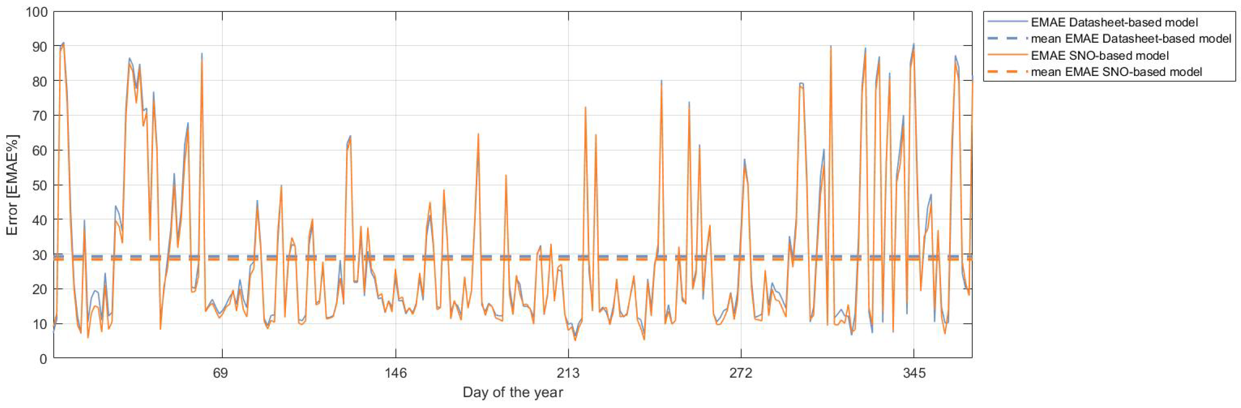
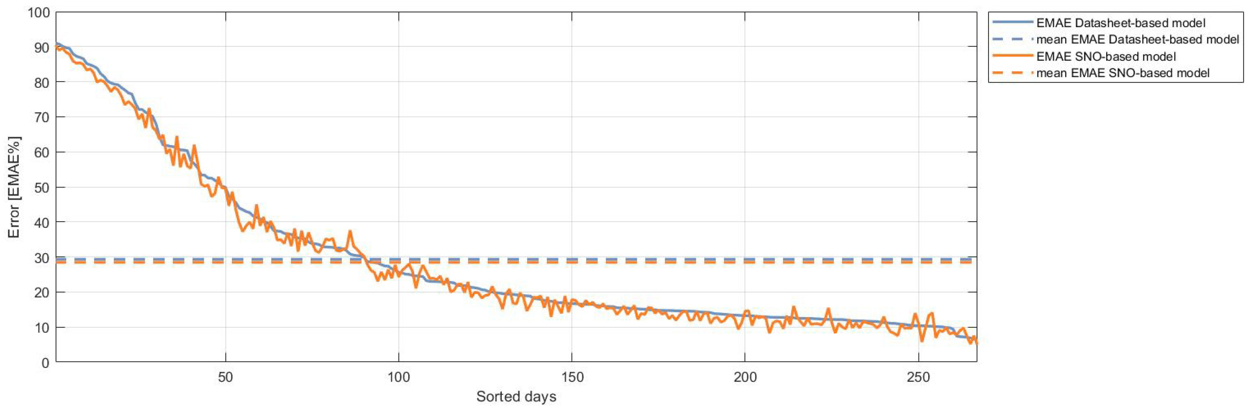
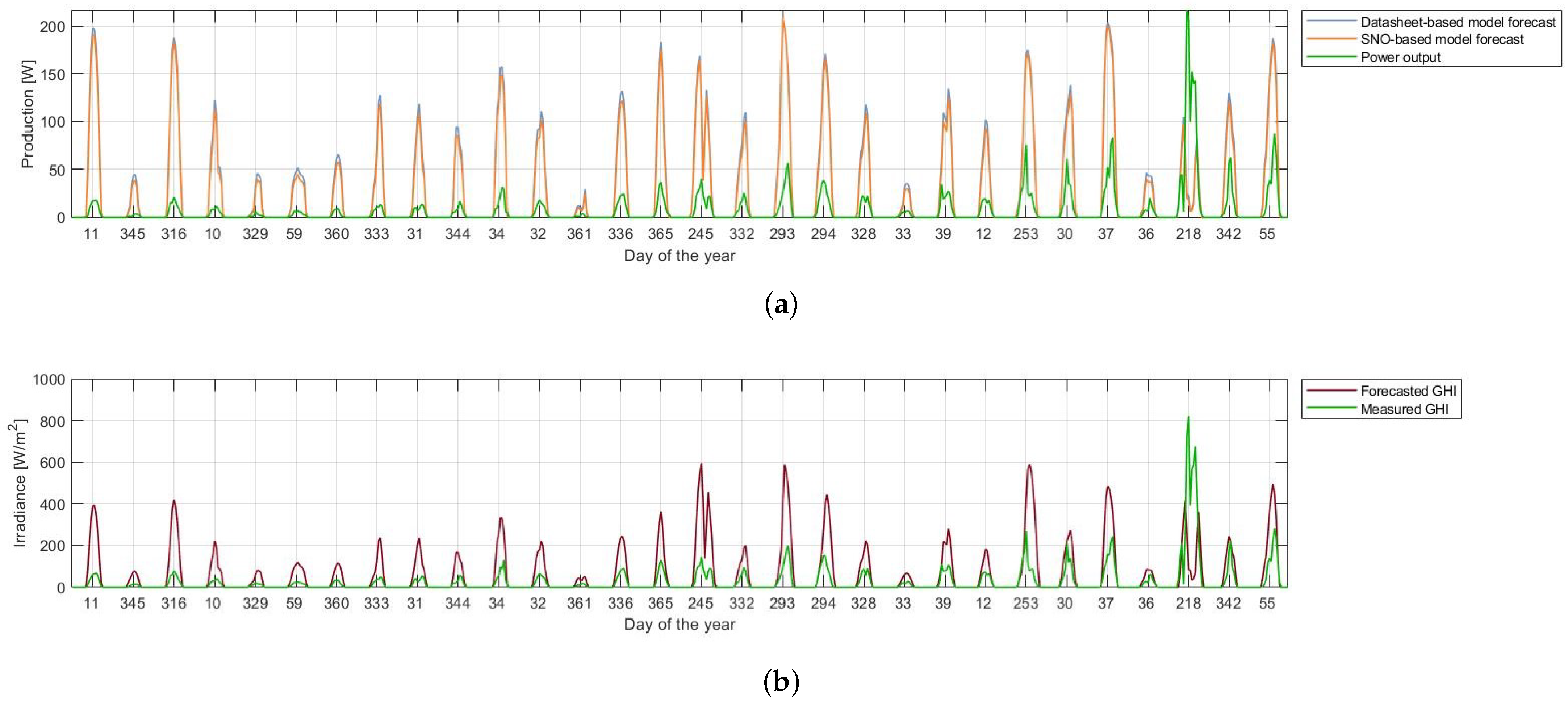
3.1. Forecasting with Physical Models

In the first analysis, the two physical models were compared.

Table 2. PV module’s electrical data. SNO: Social Network Optimization.

Parameter	Datasheet Estimation	SNO-Based Estimation
$I_{0,STC}$ (A)	1.64 $·{10}^{-8}$	2.95 $·{10}^{-6}$
$I_{PV,STC}$ (A)	9.731	8.01
n	1.259	2.0
$R_s$ ($\mathsf{\Omega }$)	0.279	${10}^{-4}$
$R_{sh,STC}$ ($\mathsf{\Omega }$)	2856.9	101.25

shows the comparison between the parameters estimated based on the datasheet information and those found by SNO in the matching procedure.

By analyzing these values, we found that those obtained from the SNO matching procedure differed greatly from those obtained from datasheets: in particular, they lost part of their physical meaning because the optimization procedure choses them also to reduce the error introduced by the weather forecast.

Figure 6 shows the envelope-weight mean average error (EMAE) comparison between the two physical models: the datasheet-based and the SNO-based models. The dashed line is the average EMAE computed for the entire year. The error made by the two physical models was similar and concentrated mainly during the winter. This phenomenon was also due to the fact that the EMAE error index was normalized with respect to the maximum between the expected power and the power actually produced. More details on the cost indexes are reported in Appendix A.

Figure 7 shows the comparison between the two techniques, sorting the days according to the datasheet-based model’s EMAE value. Even if the SNO-based model error presented some oscillations, it can be seen in most cases to have been better than the datasheet-based error, confirming the lower average value.

Most of the error was concentrated in a few days in which the forecast was highly inaccurate: only in 90 days out 268 was the error above the average. The EMAE trend is the same as the SNO-based model, showing that this can be due to inaccurate weather forecasts, which is reflected by both models as a power production error.

In order to assess this statement, the 30 worst days according to the datasheet-based model’s EMAE are plotted in Figure 8: in Figure 8a, the power forecasted by the two physical models is compared with the actual power output; in Figure 8b, the measured and forecasted GHI are compared as a reference for understanding the error sources.

In the above figure, it appears that, for almost all of the days reported, the difference between the forecasts of the two models was very low. In fact, most of the error was introduced by inaccurate weather forecasts. In particular, it can be noted that, for both models, the error was concentrated on cloudy days; i.e., days with low irradiance.

Finally,

Table 3. Numerical comparison between the two models according to average error values. NMAE: normalized mean average error; nRMSE: normalized root mean square error; OMAE: objective mean average error.

Model	NMAE	WMAE	nRMSE	EMAE	OMAE
Datasheet-based	5.25	83.32	32.61	29.34	19.80
SNO-based	4.90	74.22	29.60	28.47	18.32

shows a numerical comparison between the two models according to average error values. The performance of the SNO-based model was better than the datasheet-based model: in particular, the improvement was mainly focused on the error indices most correlated with the MAE, i.e., the cost function used in the optimization process.

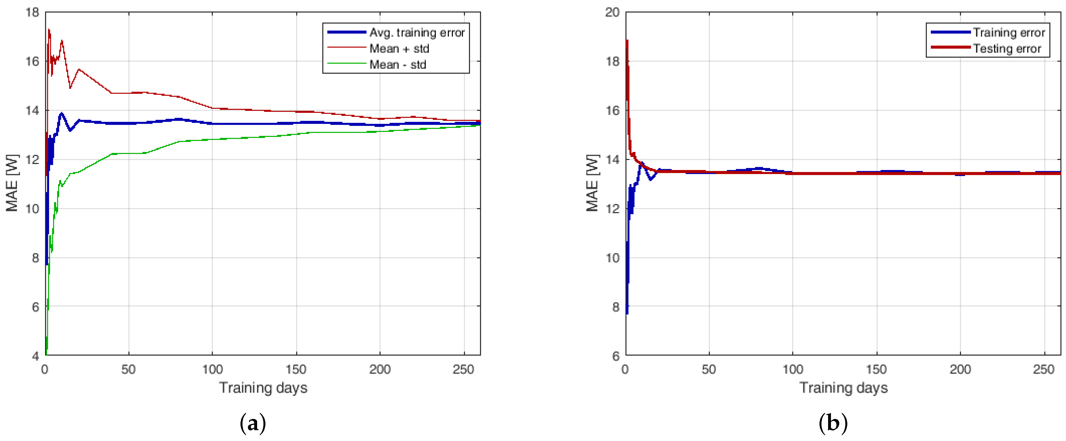
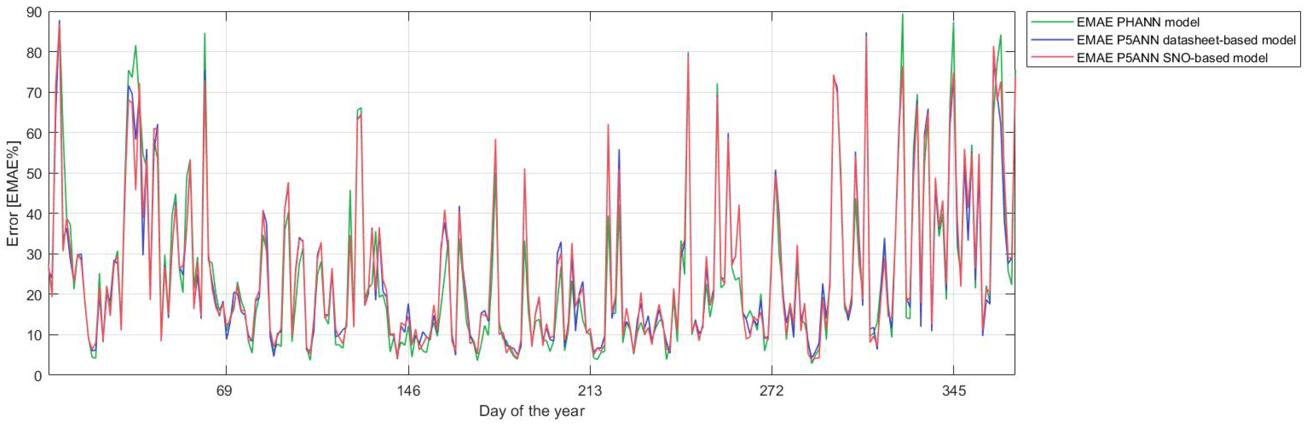
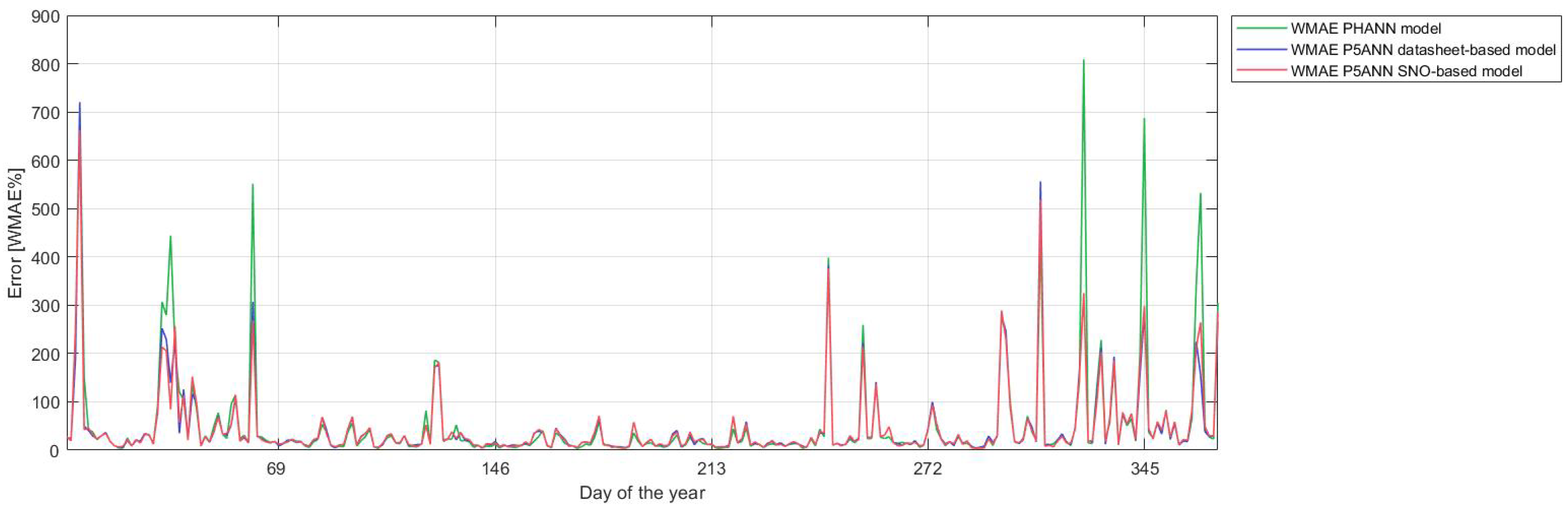
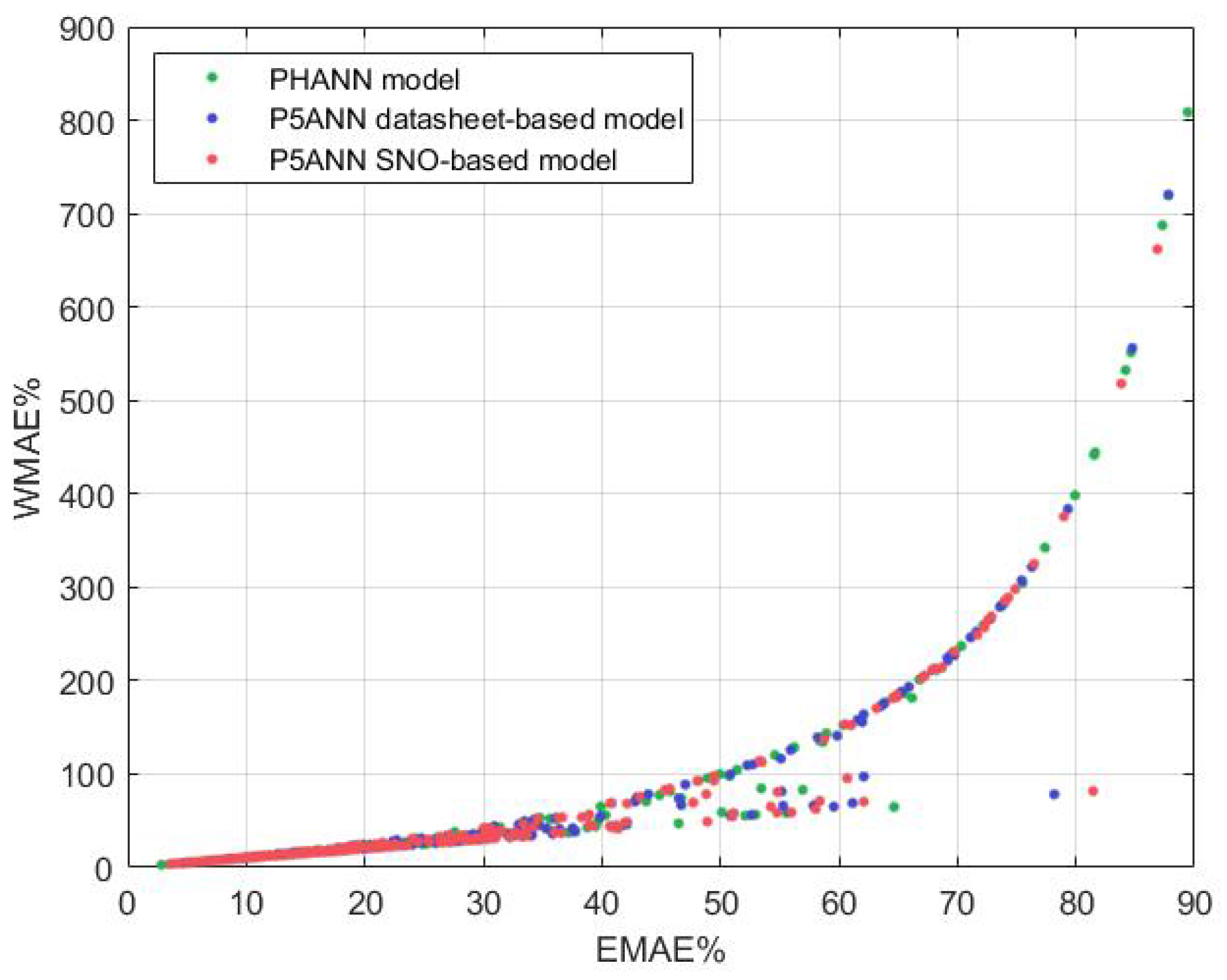
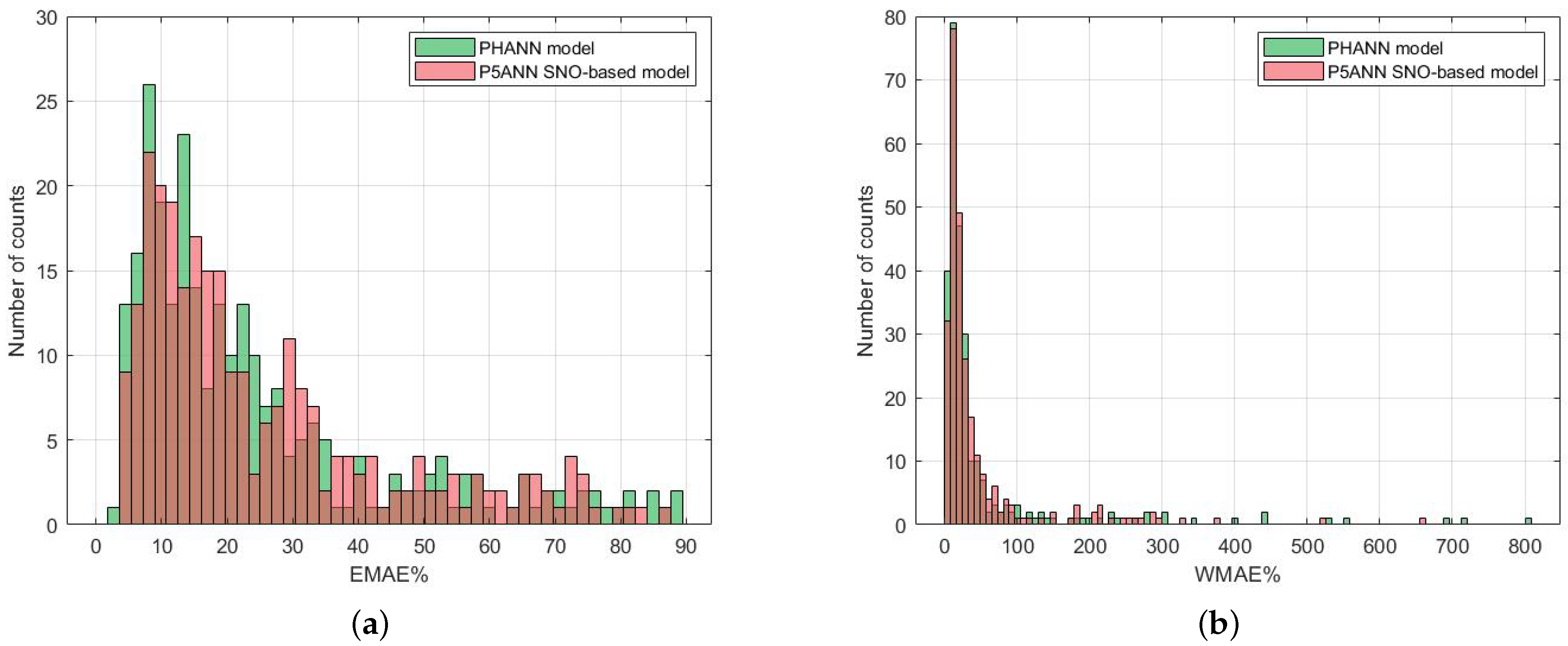
3.2. Forecasting with ANN and Hybrid Methods

In this section, the different ANN-based models are compared with respect to the described dataset.

Table 4. Numerical comparison between the four ANN-based models according to average error values.

Model	NMAE	WMAE	nRMSE	EMAE	OMAE
ANN-based	4.05	48.6	19.78	25.81	15.04
P5ANN datasheet-based	4.03	46.28	19.08	25.5	14.95
P5ANN SNO-based	4.03	46.29	18.9	25.61	15
PHANN	3.75	53.47	21.4	24.72	14.23

shows the numerical comparison between these models according to the year’s average error values. The bold values are the best achieved.

The ANN-based model achieved the worst performance for all cost indexes compared to hybrid models, which showed quite similar performances. The PHANN model achieved the lowest error value for the normalized mean average error (NMAE), EMAE and objective mean average error (OMAE), while the P5ANN model outperformed PHANN considering WMAE and considering the normalized root mean square error (nRMSE). In particular, for the latter indicator, the SNO-based P5ANN showed the best performance; however, this value may have been affected by the fact that the SNO-matching procedure was performed with MAE.

Figure 9 shows the comparison between the average daily EMAE error of the three hybrid models. Although the error was generally greater during the winter, it was still better distributed than for the physical models (Figure 6). It can thus be noted that PHANN showed an error trend that differed from the P5ANN models, which had a similar behavior: in particular, PHANN showed some peaks with very high error, while it managed to obtain better results in many days in which the EMAE was less than 30%.

A similar comparison is made in Figure 10 with respect to the daily average WMAE error. This error index further highights the peaks present in the winter period, accentuating the differences between PHANN and P5ANN. This fact explains why in Table 4 PHANN’s WMAE is significantly worse than the other two hybrid models.

To better examine the differences between these error indices, in Figure 11, the WMAE error is represented as a function of the EMAE error. Each point corresponds to the daily error made by one of the three models, which are represented with different colors. In the figure, it can be seen that there are two different relationships between these error indices: for some points, there is an almost linear behavior, while for the most part, the relationship is super-linear. This second type of relationship is responsible for the differences highlighted above: in fact, high errors increase their relevance compared to lower errors.

In Figure 12, the distributions of the EMAE (a) and WMAE (b) errors are represented by means of histograms for the PHANN and P5ANN SNO-based models. In these graphs, we see the different distributions of these errors: PHANN has a distribution with a lower median than the P5ANN SNO-based model; however, as already highlighted before, the tails are more pronounced, particularly for the WMAE error.

Finally, Figure 13 shows a comparison between PHANN and P5ANN SNO-based models on the 30 worst days of the PHANN model: in Figure 13a, the power forecasted by the two models is compared with the measured power output, and in Figure 13b, the measured and forecasted GHI are compared.

Analyszng the 30 worst days of the PHANN model, 23 were in common with the 30 worst days of the datasheet-based model. This means that the error was still mainly due to incorrect weather forecasts and that the learning capabilities of hybrid models are able only to partially compensate for this input error.

4. Conclusions

The forecasting problem for photovoltaic production can be effectively handled with hybrid models. In this paper, the performance and the specific features of three hybrid models have been analyzed on real measurement data acquired at SolarTech^LAB. The breadth of the database considered allows generality to the work carried out not to be lost, although the data are related to a single module. In particular, the characteristics of the measurement system, albeit on a different scale, are similar to the problems that can be found in a larger system.

The first two proposed hybridization strategies are based on the five-parameter physical model of a PV module: the parameters of this model have been obtained firstly from the datasheet and then from a matching procedure with the historical data and an Evolutionary Algorithm named Social Network Optimization. The third hybridization strategy is the already tested PHANN, in which clear sky irradiance has been used as the input for the neural network.

Firstly, the two physical models based on the five-parameter model of a PV modules were compared: as expected, the performance of the Social Network Optimization-based model was better thanks to the training process used for the identification of the model parameters.

Secondly, the hybrid models were compared with a basic ANN approach: the superiority of all the three hybridizations was assessed. The difference in the performances of the three hybrid models were very low and changed according to the specific error index used. This shows the importance of hybridization when applying ANN for power output forecasting, while the physical input used for the hybridization only slightly affects the final performance. This means that the hybridization source can be selected according to the available data of each specific application.

Thirdly, the performance of the PHANN and P5ANN SNO-based models were compared against two different error rates: EMAE and WMAE. From this analysis, this second indicator appears to be more affected by PHANN error peaks; on the other hand, the EMAE cost index differentiates the performances of the days with low error more clearly.

References

1. Choudhary, P.; Srivastava, R.K. Sustainability perspectives-a review for solar photovoltaic trends and growth opportunities. J. Clean. Prod. 2019, 227, 589–612. [Google Scholar] [CrossRef]
2. Dolara, A.; Grimaccia, F.; Magistrati, G.; Marchegiani, G. Optimization Models for Islanded Micro-grids: A Comparative analysis between linear programming and mixed integer programming. Energies 2017, 10, 241. [Google Scholar] [CrossRef]
3. Aziz, N.I.A.; Sulaiman, S.I.; Shaari, S.; Musirin, I.; Sopian, K. Optimal sizing of stand-alone photovoltaic system by minimizing the loss of power supply probability. Sol. Energy 2017, 150, 220–228. [Google Scholar] [CrossRef]
4. Muhsen, D.H.; Nabil, M.; Haider, H.T.; Khatib, T. A novel method for sizing of standalone photovoltaic system using multi-objective differential evolution algorithm and hybrid multi-criteria decision making methods. Energy 2019, 174, 1158–1175. [Google Scholar] [CrossRef]
5. Hashemi, B.; Cretu, A.M.; Taheri, S. Snow Loss Prediction for Photovoltaic Farms Using Computational Intelligence Techniques. IEEE J. Photovolt. 2020, 10, 1044–1052. [Google Scholar] [CrossRef]
6. Guo, M.; Zang, H.; Gao, S.; Chen, T.; Xiao, J.; Cheng, L.; Wei, Z.; Sun, G. Optimal tilt angle and orientation of photovoltaic modules using HS algorithm in different climates of China. Appl. Sci. 2017, 7, 1028. [Google Scholar] [CrossRef] [Green Version]
7. Liu, C.; Xu, W.; Li, A.; Sun, D.; Huo, H. Analysis and optimization of load matching in photovoltaic systems for zero energy buildings in different climate zones of China. J. Clean. Prod. 2019, 238, 117914. [Google Scholar] [CrossRef]
8. Titri, S.; Larbes, C.; Toumi, K.Y.; Benatchba, K. A new MPPT controller based on the Ant colony optimization algorithm for Photovoltaic systems under partial shading conditions. Appl. Soft Comput. 2017, 58, 465–479. [Google Scholar] [CrossRef]
9. Li, H.; Yang, D.; Su, W.; Lü, J.; Yu, X. An overall distribution particle swarm optimization MPPT algorithm for photovoltaic system under partial shading. IEEE Transact. Ind. Electron. 2018, 66, 265–275. [Google Scholar] [CrossRef]
10. Mao, M.; Zhou, L.; Yang, Z.; Zhang, Q.; Zheng, C.; Xie, B.; Wan, Y. A hybrid intelligent GMPPT algorithm for partial shading PV system. Control Eng. Pract. 2019, 83, 108–115. [Google Scholar] [CrossRef]
11. Hayder, W.; Ogliari, E.; Dolara, A.; Abid, A.; Ben Hamed, M.; Sbita, L. Improved PSO: A Comparative Study in MPPT Algorithm for PV System Control under Partial Shading Conditions. Energies 2020, 13, 2035. [Google Scholar] [CrossRef]
12. Dolara, A.; Grimaccia, F.; Mussetta, M.; Ogliari, E.; Leva, S. An Evolutionary-Based MPPT Algorithm for Photovoltaic Systems under Dynamic Partial Shading. Appl. Sci. 2018, 8, 558. [Google Scholar] [CrossRef] [Green Version]
13. Shareef, H.; Mutlag, A.H.; Mohamed, A. Random Forest-Based Approach for Maximum Power Point Tracking of Photovoltaic Systems Operating under Actual Environmental Conditions. Comput. Intell. Neurosci. 2017, 2017, 1673864. [Google Scholar] [CrossRef] [PubMed]
14. Petrone, G.; Luna, M.; La Tona, G.; Di Piazza, M.C.; Spagnuolo, G. Online Identification of Photovoltaic Source Parameters by Using a Genetic Algorithm. Appl. Sci. 2018, 8, 9. [Google Scholar] [CrossRef] [Green Version]
15. Xiong, G.; Zhang, J.; Yuan, X.; Shi, D.; He, Y. Application of symbiotic organisms search algorithm for parameter extraction of solar cell models. Appl. Sci. 2018, 8, 2155. [Google Scholar] [CrossRef] [Green Version]
16. Niccolai, A.; Dolara, A.; Grimaccia, F. Analysis of Photovoltaic Five-Parameter Model. In Proceedings of the 2018 International Conference on Smart Systems and Technologies (SST), Osijek, Croatia, 10–12 October 2018; pp. 205–210. [Google Scholar]
17. Louzazni, M.; Khouya, A.; Amechnoue, K.; Gandelli, A.; Mussetta, M.; Crăciunescu, A. Metaheuristic algorithm for photovoltaic parameters: Comparative study and prediction with a firefly algorithm. Appl. Sci. 2018, 8, 339. [Google Scholar] [CrossRef] [Green Version]
18. Grimaccia, F.; Leva, S.; Mussetta, M.; Ogliari, E. ANN sizing procedure for the day-ahead output power forecast of a PV plant. Appl. Sci. 2017, 7, 622. [Google Scholar] [CrossRef] [Green Version]
19. Dolara, A.; Grimaccia, F.; Leva, S.; Mussetta, M.; Ogliari, E. Comparison of Training Approaches for Photovoltaic Forecasts by Means of Machine Learning. Appl. Sci. 2018, 8, 228. [Google Scholar] [CrossRef] [Green Version]
20. Ogliari, E.; Niccolai, A.; Leva, S.; Zich, R.E. Computational intelligence techniques applied to the day ahead PV output power forecast: PHANN, SNO and mixed. Energies 2018, 11, 1487. [Google Scholar] [CrossRef] [Green Version]
21. Thong, P.H. Some novel hybrid forecast methods based on picture fuzzy clustering for weather nowcasting from satellite image sequences. Appl. Intell. 2017, 46, 1–15. [Google Scholar]
22. Socaci, I.A.; Czibula, G.; Ionescu, V.S.; Mihai, A. XNow: A deep learning technique for nowcasting based on radar products’ values prediction. In Proceedings of the 2020 IEEE 14th International Symposium on Applied Computational Intelligence and Informatics (SACI), Timisoara, Romania, 21–23 May 2020; pp. 117–122. [Google Scholar]
23. Niccolai, A.; Nespoli, A. Sun Position Identification in Sky Images for Nowcasting Application. Forecasting 2020, 2, 488–504. [Google Scholar] [CrossRef]
24. Dolara, A.; Grimaccia, F.; Leva, S.; Mussetta, M.; Ogliari, E. A physical hybrid artificial neural network for short term forecasting of PV plant power output. Energies 2015, 8, 1138–1153. [Google Scholar] [CrossRef] [Green Version]
25. Chaibia, Y.; Allouhib, A.; Malvonic, M.; Salhia, M.; Saadanid, R. Solar irradiance and temperature influence on the photovoltaic cell equivalent-circuit models. Sol. Energy 2019, 188, 1102–1110. [Google Scholar] [CrossRef]
26. De Soto, W.; Klein, S.; Beckman, W. Improvement and validation of a model for photovoltaic array performance. Sol. Energy 2006, 80, 78–88. [Google Scholar] [CrossRef]
27. Dolara, A.; Leva, S.; Manzolini, G. Comparison of different physical models for PV power output prediction. Sol. Energy 2015, 119, 83–99. [Google Scholar] [CrossRef] [Green Version]
28. Laudani, A.; Mancilla-David, F.; Riganti-Fulginei, F.; Salvini, A. Reduced-form of the photovoltaic five-parameter model for efficient computation of parameters. Sol. Energy 2013, 97, 122–127. [Google Scholar] [CrossRef]
29. Jain, A.; Kapoor, A. Exact analytical solutions of the parameters of real solar cells using Lambert W-function. Sol. Energy Mater. Sol. Cells 2004, 81, 269–277. [Google Scholar] [CrossRef]
30. IEC. EN 60891:2010-Photovoltaic Devices—Procedures for Temperature and Irradiance Corrections to Measured I-V Characteristics; IEC: Londin, UK, 2010. [Google Scholar]
31. Dainese, C.; Faranda, R.; Leva, S. Thermal Analysis for Different Types of PV Panels. In Proceedings of the Power and Energy Systems, EuroPES 2009, Palma de Mallorca, Spain, 7–9 September 2009. [Google Scholar]
32. Sera, D.; Teodorescu, R.; Rodriguez, P. PV panel model based on datasheet values. In Proceedings of the 2007 IEEE International Symposium on Industrial Electronics, Seoul, Korea, 5–8 July 2013; pp. 2392–2396. [Google Scholar]
33. Zhu, X.; Fu, Z.; Long, X.; Xin-Li. Sensitivity analysis and more accurate solution of photovoltaic solar cell parameters. Sol. Energy 2011, 85, 393–403. [Google Scholar] [CrossRef]
34. Niccolai, A.; Grimaccia, F.; Mussetta, M.; Zich, R. Optimal task allocation in wireless sensor networks by means of social network optimization. Mathematics 2019, 7, 315. [Google Scholar] [CrossRef] [Green Version]
35. Ogliari, E.; Nespoli, A. Photovoltaic Plant Output Power Forecast by Means of Hybrid Artificial Neural Networks. Adv. Struct. Mater. 2020, 128, 203–222. [Google Scholar] [CrossRef]
36. SolarTechLAB at Politecnico di Milano. Available online: http://www.solartech.polimi.it/ (accessed on 2 December 2020).
Figure 1. Equivalent circuit of single diode five-parameter model.
Energies 14 00451 g001
Figure 2. Scheme of the matching procedure with Social Network Optimization.
Energies 14 00451 g002
Figure 3. Convergence curves with 20 training days. The thicker red line corresponds to the average converge, while the gray lines represent the 40 independent trials performed.
Energies 14 00451 g003
Figure 4. Effect of the selection of the training days. (a) Variability of the solutions: average value, first and third quartiles. (b) Learning curves, where each point is the average of 40 independent trials.
Energies 14 00451 g004
Figure 5. Schematic view of P5ANN (hybrid of a five-parameter equivalent model and the Artificial Neural Network): the network receives as inputs the weather forecast and the corresponding power output of the five-parameter models.
Energies 14 00451 g005
Figure 6. Envelope-weight mean average error (EMAE) comparison between the two physical models: the datasheet-based and the SNO-based models. The dashed line is the average EMAE computed for the entire year.
Energies 14 00451 g006
Figure 7. EMAE comparison between the two physical models, in which the days are sorted according to the error value.
Energies 14 00451 g007
Figure 8. Comparison on the 30 worst days of the datasheet-based model with respect to (a) the forecasted power of the two physical models and (b) the forecasted and measured GHI.
Energies 14 00451 g008
Figure 9. EMAE comparison for the three ANN-based hybrid models.
Energies 14 00451 g009
Figure 10. WMAE comparison between the three ANN-based hybrid models.
Energies 14 00451 g010
Figure 11. Scatterplot of EMAE and WMAE values obtained from the three hybrid models.
Energies 14 00451 g011
Figure 12. Histogram for the errors of the PHANN and the P5ANN SNO-based models: (a) EMAE and (b) WMAE.
Energies 14 00451 g012
Figure 13. Comparison of the 30 worst days of the PHANN model between (a) the forecasted power of the PHANN and P5ANN SNO-based models, and (b) the forecasted and measured GHI.
Energies 14 00451 g013