A Novel Application of Ensemble Methods with Data Resampling Techniques for Drill Bit Selection in the Oil and Gas Industry

Abstract

Selection of the most suitable drill bit type is an important task for drillers when planning for new oil and gas wells. With the advancement of intelligent predictive models, the automated selection of drill bit type is possible using earlier drilled offset wells’ data. However, real-field well data samples naturally involve an unequal distribution of data points that results in the formation of a complex imbalance multi-class classification problem during drill bit selection. In this analysis, Ensemble methods, namely Adaboost and Random Forest, have been combined with the data re-sampling techniques to provide a new approach for handling the complex drill bit selection process. Additionally, four popular machine learning techniques namely, K-nearest neighbors, naïve Bayes, multilayer perceptron, and support vector machine, are also evaluated to understand the performance degrading effects of imbalanced drilling data obtained from Norwegian wells. The comparison of results shows that the random forest with bootstrap class weighting technique has given the most impressive performance for bit type selection with testing accuracy ranges from 92% to 99%, and G-mean (0.84–0.97) in critical to normal experimental scenarios. This study provides an approach to automate the drill bit selection process over any field, which will minimize human error, time, and drilling cost.

1. Introduction

Oil and gas wells are drilled from the surface of the Earth to underlying hydrocarbon reservoirs. The whole drilling operation is carried out through a mechanical drill string which contains a drill bit installed at its lower tip for crushing the rock layers. These drill bits are normally worn out due to wear and tear over time as they move forward inside the formation. Drill bits are changed regularly through tripping operations in the oil and gas industry. These drill bits are costly in nature and needed to be properly selected as they may represent up to 10–40% of the dryhole cost of the wellbore [1]. The average cost of drilling a well varies from 4.9 million to 650 million U.S. dollars depending upon the type of wells. However, overall expenditures for drilling an oil well are needed to be minimized for achieving cost-effective drilling operations. The cost of drilling operation for a hydrocarbon well is mainly dependent on various factors namely, the operating cost of the drill rig, the time required for drilling target formations, the number of tripping operations, life of the drill bit, and drill bit cost [1]. Still, drilling costs can be significantly minimized through the selection of appropriate drill bit designs which in turn reduces the operating time of the rig with less tripping events and more life expectancy of the drill bit. Moreover, the selection of suitable drill bit types for drilling geological formations is a problematic task due to complex interactions between reservoir properties, drill string hardware design, and various operational parameters [2]. Thus, the selection of appropriate drill bit type is an important task for drilling engineers while planning for new oil and gas wells.

With the advancement of sensor-based measurements, a large amount of well data are being generated during field operations such as measurement-while-drilling, logging-while-drilling, etc. [3]. However, the automated selection of drill bit type is possible using earlier drilled offset wells’ data. These data are highly complex with the problem of nonlinearity, high dimensionality, noise, and imbalance in nature [3,4]. Therefore, the interpretation of wells data has become difficult for conventional techniques that are unable to process the bulk amount of data and make fast decisions for drill bit type selection. Various researchers have proposed empirical and data-driven models to correlate complex drilling variables for drill bit selection as described briefly in the next section. The remaining paper is organized as follows: Section 2, presents a literature review. Section 3, briefly describes the various data-driven models utilized in this work. Section 4, explains the research methodology adopted in the paper, whereas Section 5, contains results and discussion. Finally, the Section 6, concludes the major findings of the research work along with future scope.

2. Literature Review

Several researchers have suggested various empirical correlations for the selection of appropriate drill bit types. One of the most popular conventional methods for the selection of drill bits is cost per foot (CPF) [5]. CPF can be calculated as given below:

$$CPF=\frac{C_{BIT}+C_{RIG}(T_{br}+T_{co}+T_t)}{L_D}$$

(1)

where C_BIT is the cost of bit in dollars, C_RIG is the cost of operating drill rig per hour, T_br is run time of the drill bit, T_co is the connection time, T_t is tripping time in hours, and L_D is the length of the drilled interval. The main drawback of CPF is that it does consider the drilling variables and formation type which directly and indirectly affects drill bit life. This method can’t be utilized for drilling the directional and horizontal wells [5]. The second method for bit selection is based on the calculation of specific energy (S_E) which is required to remove the unit volume of rock during drilling operations [6]. S_E can be determined as given below.

$$S_E=\frac{RPM\ast WOB}{ROP\ast BD}$$

(2)

where RPM is rounds per minute (rpm), BD is the diameter of bit (ft), WOB is the weight on bit (lb), and ROP is the penetration rate (ft/h). This Equation (2) has considered only three important drilling parameters but ignored the rock mechanics and vibrational impacts on the dullness grading of the drill bit. Further, the International Association of Drilling Contractors (IADC, Houston, TX, USA) suggested the use of bit dullness for selecting the roller cone as well as fixed cutter bits. Eight diverse parameters were utilized to describe the dull bit conditions. Diverse conditions were assigned from one to eight codes symbolizing the degree of dullness existing in a drill bit [7]. However, this technique has a major drawback that requires human visual expertise for the evaluation of drill bit conditions. Thus, the chances of human error are high in this dill bit selection technique.

In 1964, Hightower attempted to select drill bits based on the geological information and drilling data obtained from previously drilled offset wells [8]. He utilized sonic logs to define formation drillability to select suitable drill bit types for drilling new geological formations [8]. However, he did not determine the rock strength directly but indirectly estimated it through the theory of elasticity. Mason [9] utilized sonic logs, offset wells data, and lithological information for the selection drill bit type. Perrin et al. [10] proposed a drilling index to evaluate the performance drill bit that was also applicable for horizontal and directional drilling operations. Mensa-Wilmot et al. [11] suggested a new formation drillability parameter for drill bit evaluation and integrated several rock mechanics parameters in it. Xu et al. [12] modified the equation of CPF using mud logging data which was found to be more efficient than the conventional CPF equation for the selection of drill bit [12]. Uboldi et al. [13] conducted micro indentation tests on the cuttings of subsurface rock layers to determine the mechanical characteristics of subsurface rock layers. Further, they estimated the compressive index of rock formations along with lithological data which were then utilized by a Drill Bit Optimization System to help the driller for drill bit selection [13]. Sherbeny et al. [14] used wellbore images and mineralogy logs for the selection and design of drill bits. Mardiana and Noviasta [15] combined rock strength analysis and finite element modeling for the selection of drill bits. Cornel and Vazquez [16] utilized bit dullness data for the selection of optimum drill bit types for different geological formations. They also optimized the PDC bit design and drilling hydraulics to identify optimum operational parameters.

With the advancement of sensor-based measurements, a large amount of wells data are being generated during field operations such as measurement-while-drilling, logging-while-drilling, etc. The interpretation of wells data has become difficult for conventional techniques that are unable to process the bulk amount of wells data and make fast decisions for drill bit type selection. Thus, smart computational models are applied for the processing of big wells data to select suitable drill bit types. Several researchers have suggested the utilization of machine learning models as an alternative approach for the automatic selection of drill bit types based on previously drilled offset wells data. In 2000, Bilgesu et al. [1] applied artificial neural networks (ANN) for the selection of drill bit types to drill various formations but they failed to include the reservoir properties in their training data. Further, Yilmaz et al. [17] employed the ANN model for the selection of drill bit type. They selected bit type based on the desired values of the rate of penetration (ROP) and other drilling variables. They also showed that ANN based models were good only for providing initial suggestions regarding the drill bit type when tested for diverse field conditions [17]. Edalatkhah, Rasoul, and Hashemi [18] applied ANN and Genetic algorithm (GA) for the choice of bit types based on desired and optimum values of drilling ROP. Hou, Chien, and Yuan, [19] applied ANN for the screening of polycrystalline diamond compact (PDC) drill bits trained on offset wells data, drillability and lithofacies information. Nabilou [20] studied the impact of drill bit selection parameters especially geo-mechanical factors in a case study of an oil and gas reservoir existing in the southwest part of Iran. Efendiyev et al. [21] selected run speed and cost of the drill bit as significant criteria for the selection drill bits. Momeni et al. [22] applied ANN for the prediction of drill bit types based on the offset wells drilling data and predicted ROP values by adding predicted drill bit types in the training dataset. Abbas et al. [23] selected drill bit types based on the optimum values of ROP using ANN and GA. Manuel et al. [24] selected drill bits types for different geological depths using image processing techniques, principal component analysis (PCA), and ANN. Most of the abovementioned research works are trained on the balanced datasets with less number of drill bit types. The successful applications of ANN have shown that data-driven models have the potential for the automation of the bit selection process. However, none of them have considered the problem of imbalanced data that will naturally occur due to the varying thickness of subsurface lithofacies. The actual field data contain the uneven distribution of data samples that result in a complex imbalance multiclass classification problem during drill bit selection. This uneven distribution of training data samples affects the generalization capability of supervised machine models for unseen data and also make them unreliable. Here, the generalization of machine learning models means that the trained models provide their best possible performance results for unseen testing data also. Therefore, proper investigation of machine learning models is required to evaluate their effectiveness for the screening of drill bit types with complex offset wells data to provide more pragmatic solutions.

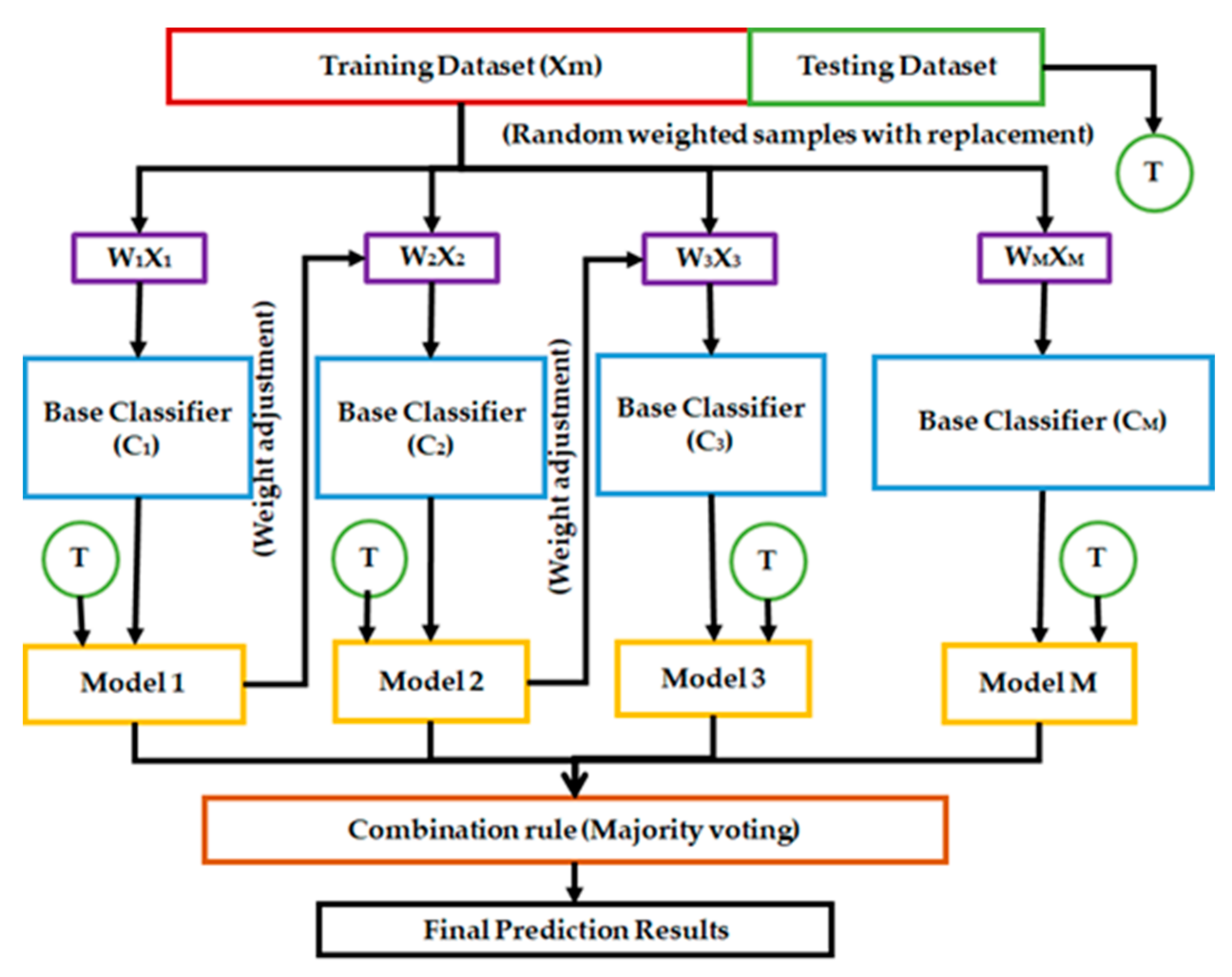
Here, the drill bit selection process has been formulated as a multiclass classification problem where diverse drill bit types have acted as class labels. In this paper, two ensemble methods namely, AdaBoost and random forest (RF) have been investigated for handling the complex multiclass imbalanced data problem associated with intelligent drill bit selection. These ensemble paradigms contain boosting techniques in its internal architecture which has been reported useful for solving the imbalanced data issues. They also reduce the bias and variance error associated with training data that provide a better generalization to the prediction results. These ensemble methods are combined with data resampling techniques to enhance their capability of dealing with imbalanced data. Additionally, the behavior of four popular classifiers namely, K-nearest neighbors classifier (KNC), naïve Bayes classifier (NBC), multilayer perceptron (MLP), and support vector classifier (SVC), have also been studied to select diverse bit types for drilling critically unstable geological formations. The abovementioned popular classifiers have also been tested to study the impact of imbalance and establish the supremacy of the proposed approach. The primary motivation of this research work is to explore popular machine learning algorithms in quest of higher drill bit selection accuracy and better generalization. The primary objectives of this study are given below:

(1)

The applicability of intelligent models for drill bit selection has been reviewed.

(2)

Ensemble models are investigated in quest of higher bit selection accuracy.

(3)

A comparative study of popular machine learning models has been performed for drill bit selection.

(4)

The problem of imbalanced data is addressed in this work that adversely affects the performance of machine learning models for the selection of the drill bit.

(5)

The impact of softer and unstable geological formations that produce critical training data for machine learning models have been discussed to select diverse drill bit types.

(6)

The behavior of machine learning models has also been studied for drill bit selection in critical formations.

(7)

The future implications of this work are elaborated for automatic drill bit selection.

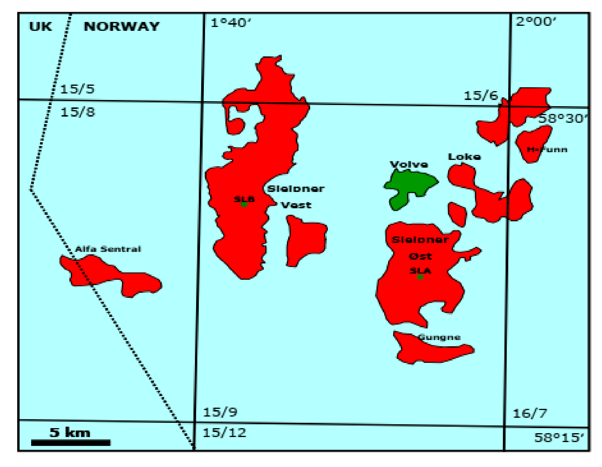
The comparison of results has been performed to identify the best performing classifier among all the above-mentioned models. All the applied machine learning models have been trained and tested using Norwegian oil and gas field data. The data related challenges associated with the drill bit selection process have also been discussed. This paper discusses issues related to intelligent classifiers and imbalanced petroleum data such as applicability issues, performance difficulties, performance evaluation parameters, and possible data-driven solutions. Overall, a comprehensive study of machine learning models has been performed to assess the challenges associated with the automatic drill bit selection process with practical field datasets.

3. A Brief Description of Applied Models

In this study, oversampling and undersampling approaches have been utilized to generate the balanced datasets for the training and testing of ensemble methods. All the data related techniques used in this research work are briefly explained below.

3.1. Data Resampling Techniques

Several real-world problems involve imbalanced data issues where the distribution of samples varies from class to class. It is reported that the majority classes naturally dominate the minority classes during the training of supervised classifiers, which makes them biased and unreliable. However, machine learning models require balanced datasets for their best possible performance [25]. To overcome this imbalanced data problem, two data sampling techniques were applied for generating balanced datasets for the classifiers to compensate for the ill effects of imbalanced data.

3.1.1. Oversampling

Oversampling technique increases the data samples in the minority class by duplicating the prevailing samples or producing synthetics ones [26]. This approach is widely applied for the generation of the balanced dataset for the training of supervised classifiers. Various oversampling techniques are available in the literature such as random over sampler, focus over sampler, synthetic minority over-sampling technique (SMOTE), etc. SMOTE is a widely applied technique for oversampling. Therefore, in this paper, the SMOTE technique has been applied for balancing the number of data samples for each class. This approach does not produce duplicate copies of existing data samples but synthesizes new ones. It takes the feature space samples for each class and combines them with the features of nearest neighbors [26,27].

3.1.2. Undersampling

In the undersampling technique, the samples from the majority class are removed to decrease their data samples up to the number of minority class’s data samples. This seems to be a straightforward approach for data sampling but is found suitable when the minority class has a sufficient amount of data samples [28]. There are various techniques applied for undersampling of the data samples such as Tomek links, edited nearest neighbors, random under sampler, etc. [27,28]. The random under sampler technique has been used for the generation of balanced dataset used in this study. It’s a simple and fast method for the generation of a balanced dataset through random sampling from original data. Here, the number of samples in each class of balanced dataset is predefined by the user. This technique selects bootstrap subsets from the original data for each class based on the user-defined value of samples [27]. It considers each class independently in case of multiclass imbalance problems which is useful for sampling heterogeneous data having string values in samples [27,28]. Undersampling approach has been recommended only in big data conditions and may result in loss of important information during removal of data samples from the majority class [27,28]. Both over and under-sampling approaches have limited benefits for handling imbalanced data at the data level, therefore, ensemble methods, having boosting techniques in their internal architecture, are also investigated at the algorithm level to compensate for the effects of imbalance.

3.2. Ensemble Methods

Ensemble methods are multiple-learner-systems that train and combine the outcomes of several supervised learners to produce the outcomes for pattern recognition tasks [29]. The motivation for the integration of supervised machine learning models is to achieve higher prediction accuracy and improve the generalization ability of ensemble models. The ensemble approach has been reported to be efficient for reducing errors associated with the bias and variance of training data [29]. These methods are also found suitable for handling imbalanced data problems because they integrate boosting techniques within their internal architectures [29,30]. In this study, two ensemble methods namely, AdaBoost and random forest are mainly studied for handling complex imbalanced data for the drill bit selection process. The two ensemble methods are briefly explained below.

3.2.1. Adaboost

Freund and Schapire [31] proposed an AdaBoost ensemble technique based on the boosting paradigm. It trains the base classifiers using random bootstraps data samples generated from original data and combines their decisions through a weighted majority vote. Initially, it assigns equal weights to all the training data samples [30,31]. Further, weight adjustments are performed based on the misclassifications obtained through the initial base classifier. Weights of misclassified data samples are increased in the next modified training dataset so that the chances of occurrence of misclassified samples will be increased in the next training dataset [30]. AdaBoost is particularly found supportive in handling imbalanced data problems [32]. The assignment of weights to bootstrap subsets is equivalents to resampling data space while combining upper and downsampling [32]. It has accuracy oriented approach and focuses on the wrongly classified samples while increases the weight until it gets correctly classified. It provides a solution for an imbalanced data problem at the data level equivalent to the resampling technique utilized for imbalance reduction. In this, under-sampling of majority classes is performed to produce the balanced dataset and is termed as under-sampled AdaBoost (USA). Figure 1 depicts a generalized workflow of the AdaBoost algorithm. The standard AdaBoost ensemble can be applied as given below in Algorithm 1 [31].

Algorithm 1 [31]

Produces bootstrap training subsets $(X_n=X_1,X_2,\dots ,X_N)$ from original training data X and is associated with initial equal weights $(W_n=W_1,W_2,\dots ,W_N).(\mathrm{n}=1,2,3,\dots ,\mathrm{N})$ Base classifiers $C_n(x)$ are trained using weighted training subsets $(W_n{X}_n=W_1{X}_1,W_1{X}_2,\dots ,W_N{X}_N)$ and determine error probability as $Erro{r}_n=\frac{1}{N}{\displaystyle \sum _{i=1}^N{W}_i{\beta }_i}$ where ${\beta }_i=\left\{{}_{0ifsamplecorrectlyclassified}^{1otherwise}\right.$ and change in weights is given as $C_n=\frac{1}{2}\log \left(\frac{1-Erro{r}_n}{Erro{r}_n}\right)$ Update weights as $w_i^{n+1}=w_i^n\exp (C_n{\beta }_i^n)$ if the calculated error is between 0 to 0.5 (i = 1, 2, 3…, N) and renormalizes samples’ weights so that ${\displaystyle \sum _{i=1}^N{W}_i^{n+1}=N}$ otherwise initialize all the subsets’ weights as 1 and repeat the above-given steps. Integrate the decisions of all the classifiers $C_n(x)$ by weighted majority voting rule as specified below. $\varphi (x)=\underset{y\in \left\{-1,1\right\}}{\arg \max }{\displaystyle \sum _n}{C}_n{\theta }_{\mathrm{sgn}}(C_n(x)),\mathrm{Y}$, where ${\theta }_{i,j}={\{}_{0i\ne j}^{1i=j}$ is known as the Kronecker symbol, and Y is the class labels.

3.2.2. Random Forest (RF)

Breiman developed the RF algorithm by modifying the bagging ensemble [33]. RF can be employed for resolving estimation, detection, and recognition related problems. RF has certain peculiar merits over other classifiers such as computationally fast, few numbers of model parameters for tuning, easier evaluation of generalization error, the capability of handling high dimensionality, can be utilized for attribute selection, etc. [34]. RF is the assembly of decision trees in single ensemble architecture where each decision tree is generated from random training variables [34]. For the training of its decision trees, RF generates random bootstrap data subsets from training data with the replacement of data samples. The final estimation function is in the form of a loss function that is required to be minimized [34]. All the feature space is available to the root node of the decision tree. Non-splitting nodes in the decision tree are called terminal nodes. The standard RF algorithm can be utilized for imbalanced data classification by adjusting the weight of each class while computing the impurity score for a selected split point [35,36]. The weights will be adjusted according to the inverse relationship with class frequencies in the training data [35,36]. This will shift the focus of RF on the minority class samples. This will result in the formation of a weighted class RF technique (WCRF) for the classification of imbalanced data [35]. The second approach that can be applied with RF is the bootstrap weighting approach. Here, the weight adjustment of a class is performed based on its distribution in every bootstrap sample in place of the whole training dataset [35,36]. Such a configuration of RF is known as RF with bootstrap class weighting (WBCRF). In the third approach, the majority of classes are randomly under-sampled in bootstrap samples to produce balance datasets (USCRF). This adjustment will explicitly vary the class distribution inside the random bootstrap samples. Figure 2 shows a generalized workflow of RF algorithm.

4. Methodology

In this paper, drill bit selection has been formulated as a classification problem where diverse bit types have acted as class labels. The performance of four popular classifiers namely, KNC [37], NBC [38,39], MLP [40], and SVC [41,42], have been tested to select drill bits for the given values of operational field variables. AdaBoost and RF are also applied with the resampling technique for screening of drill bit. All the machine learning paradigms have been implemented through the open-source Scikit-Learn version 0.24 and Python 3.8.0 package on the Anaconda 3 2020.11 platform. Python libraries have several merits over other prevailing platforms such as the capability of handling real-field input wells data, implementation of statistical tests to intelligent paradigms, visualization of results, self-explanatory user guides, community, and forums, etc. This whole study was carried on a 10th generation Intel Core i7-1065G7 processor with the hardware and software configurations, namely 8 MB Cache, GHz, four cores, 16 GB RAM, 8 GB graphic cards and the Windows 10 operating system.

4.1. A Brief Description of the Volve Field

This field is situated in the central part of the North Sea near the Norwegian Continental Shelf. It was discovered in 1993 and its production shut down in 2016 by its investors’ companies. The ocean depth near the Volve field is in a range of 85 to 95 m. This field contains Jurassic sandstone related to the Hugin formation reservoir. Figure 3 shows the location of the Volve oil and gas field in the North Sea. The depositional environment of this reservoir is analyzed as tidal to the shallow estuary [43]. The sandstones of the Hugin reservoir contain high contents of quartz and a medium to low range of mica and clay minerals. Various faults can also be found in Hugin formation due to salt and Jurassic extensional tectonics [43]. Draupne formation acts as a worthy spring for oil production due to its organic-rich claystone layer. Smectite contents and argillaceous clay are found in large quantities in Hordaland shales which may be the cause for the higher formation pore pressure and its instability. This formation is not recommended for drilling high angle wellbore due to its easy collapse chances [43]. Balder formation comprises crumbly tuff content which has been reported as the primary reason for mud losses and washouts. The presence of crumbly tuff in Blader formation also decreases its fracture gradient that leads to the instability of formation. Drilling operations in the Sola formation has also suffered from several issues such as a tight hole, collapses, etc. The average properties expected from this Hugin reservoir are as follows: porosity (0.2), permeability (910), water saturation (0.23), and shale volume (0.17) [43]. Geosteering was particularly utilized to increase the extent of the reservoir linking to various fault blocks.

Table 1. Geological prognosis of Well 15/9-F-12 under study (courtesy: Equinor company) [43].

Group	Formation	Depth (m)	Description
Nordland	Utsira Top	892	Grey claystone, a stringer of sand and siltstone.
	Utsira Base	1084	Well sorted sandstone, minor silt, and limestone stringers.
Hordaland	Skade Top	1259	Claystone, minor limestone/dolomite stringers.
	Skade Base	1347	Medium-grained sorted sandstone.
	Grid Top	2179	Fine-grained sandstone.
	Grid Base	2245	Fine-grained sandstone.
Rogaland	Balder Top	2317	Colored claystone, partly tuffaceous, and limestone stringers.
	Sele Top	2374	Claystone and limestone stringer.
	Lista Top	2445	Non-calcareous claystone and minor limestone stringers.
	Ty Top	2531	Fine to medium sandstone some interbedded claystone, siltstone, and limestone stringers.
Shetland	Ekofisk Top	2698	Limestone with traces of claystone and sandstone.
	Tor Top	2715	White limestone with traces of claystone.
	Hod Top	2839	Limestone along with gluconate.
	Blodoeks Top	2944	Marl, argillaceous laminations, and gluconates in parts.
	Hidra Top	2972	Off-white firm limestone.
Cromer Knoll	Roedby Top	2981	Marl along with argillaceous laminations
	Aasgard Top	3001	Interbedded limestone and marl with minor claystone and siltstone.
Viking	Draupne Top	3036	Organic-rich claystone, micaceous, carbonaceous with traces of pyrite.
	Heather Top	3086	Claystone with limestone stringers.
Vestland	Hugin Top	3094	Sandstone and rare claystone stringers.
	Sleipner Top	3266	Sandstone, grey claystone, and layers of coal.

contains the geological prognosis of Well 15/9-F-12 considered under this study.

4.2. Data Description

The dataset utilized for training and testing of machine learning models belonged to Norwegian Volve oil and gas fields. These data are available online and can be downloaded from the website of the Equinor oil and gas company. The field data of the fourteen Volve oil and gas wells were made public for academic and research purposes in 2018 [43]. Eight wells data were downloaded from the Equinor company website for the testing of machine learning models considered in the study for drill bit selection namely, 15/9-F-4, 15/9-F-5, 15/9-F-7, 15/9-F-9, 15/9-F-10, 15/9-F-11, 15/9-F-14, and 15/9-F-15 [43]. These wells were planned to maximize the production of hydrocarbon from the Hugin formation. Generally, the production wells in the Volve field were multilateral in nature, however, observation and injection wells were in J-shape trajectory [43]. The total number of data points extracted from the final drilling reports of eight wells are shown in

Table 2. Details of data samples extracted from the Final drilling reports of Norwegian wells.

S. No.	Well No	Data Samples	Classification
1.	F-4	548	Injector well
2.	F-5	721	Injection Well
3.	F-7	187	Production well
4.	F-9	180	Production well
5	F-10	718	Observation/Production well
6.	F-12	631	Production well
7.	F-14	711	Production well
8.	F-15	616	Observation well
	Total	4312

.

Oil and gas wells are drilled from the earth’s surface to the target depths of geological rock formations through drilling rig assembly. Mechanical drill strings are installed at the drill site containing drill bits at its bottom tip for crushing the subsurface rock layers. To control and monitor the oil and gas field operations efficiently, various sensors are installed on the drill rig and string to capture five types of variables namely seismic parameters, operational parameters, mud logging parameters, well logging parameters, and formation characteristics parameters [44].

Table 3. Statistical details of collected drilling data of eight wells used in this study.

S. No.	Input Variables	Range	Units
1.	Measured Depth (DT)	45–3785	m
2.	True Vertical Depth (TVD)	150–3244.36	m
3.	Rate of Penetration (ROP)	1.62–205.01	m/h
4.	Weight on bit (WOB)	−7.27–51.57	tons
5.	Rounds per minutes (RPM)	6–311	rpm
6.	Torque (TQ)	−28.53–96.14	kNm
7.	Standpipe pressure (SPP)	3–389.2	bar
8.	Mud weight (MW)	0.99–1.47	s.g.
9.	Flow Rate in (FR)	432–5345	L/min
10.	Total Gas (TG)	0–10.6	%
11.	Bit type (BT)	1–19	--
12.	Bit Size (BS)	8.5–26	inch
13.	D-exponent (DEXP)	0.26–1.55	--
14.	Total flow Area (TFA)	0.663–1.51	inch2
15.	Mechanical Specific Energy (MSE)	2213.0–85,127.7	psi
16.	Depth of Cut (DC)	2.5–5.06	m/rev
17.	Drill bit Aggressiveness (DBA)	2.07–6.13	--

contains the statistical description of operational and mud logging parameters utilized for the selection of drill bit types. Weight on bit (WOB), rounds per minute (RPM), torque (TQ), rate of penetration (ROP), bit type (BT), and bit size BS are drilling operational variables recorded from sensors installed on rotary drill string assembly. WOB is the downward force applied on the drill bit for crushing the rock layer through the weight of drill string assembly along with heavy drill collars. RPM contains the rotational speed of the drill string along with the depth of the geological lithology. TQ is the rotational force applied from the drill string on the rock formations. ROP is the speed of the drill bit at which it moves inside the rock formation. BS and BT are planned and recorded before the drilling operations for cutting the subsurface lithofacies. Similarly, circulating drilling mud properties are also recorded during drilling operations through mud logger equipment to understand the state of underlying rock formations and drill bit. Here, standpipe pressure (SPP) is overall pressure loss in the mud circulating system because of friction offered to the mudflow during the drilling operation. Mudflow rate (FR) is the speed of circulating drilling mud. Mud weight (MW) is the density of mud circulating as drilling fluid. Measured depth (MD) and true vertical depth (TVD) represent the depth at which the drill bit is cutting the underlying rock surfaces.

The input data extracted from the final drilling reports of eight wells contained a variety of sensor measured variables. The downloaded data are available in pdf format that has been later converted to excel file format for ease of handling. This type of data normally contains issues such as noise, redundant attributes, missing or garbage values, etc. that are required to be cleaned before uploading into machine learning models, otherwise, it will affect models’ performance. These input variables will act as predictor variables and unique IADC codes of drill bits will act as class labels. However, IADC bit numbers cannot be directly utilized for class labels instead coded to newer class labels as shown in

Table A1. Different drill bit utilized for drilling of Volve wells at different depths.

Wells	Depth In-Out (m)	Bit Type	IADC Code	Bit Size (Inch)
F-4	260–1360	1	M115 PDC	17.5
	1360–2770	2	M422 PDC	12.25
	2770–3510	3	M222 PDC	8.5
F-5	230–1415	4	M115 PDC	17.5
	1415–2930	5	M223 PDC	12.25
	2930–3785	6	M323 PDC	8.5
F-7	217–307	1	M115 PDC	17.5
	915–1080	6	M115A PDC	12.25
F-9	216–918	10	Smith XR+VEC MTMZ2069	17.5
F-10	146–207	7	XR+VEC MZ25069	36
	207–1400	8	XR+MG04B	26
	1400–1463	9	Reed RSRT16M-C9	17.5
	1463–2616	9	Reed RSR716M-C9	17.5
	2616–2825	10	Smith MDI716	12.25
	2825–3319	10	SmithMDI716	12.25
	3319–3442	11	Reed Hycalog RSX8195219S960	12.25
	3442–3695	9	Reed Hycalog RSR716D	8.5
	3695–4911	13	Reed Hycalog RSR816H-C1	8.5
	4911–5311	13	Reed Hycalog RST816H-C1	8.5
F-12	365–1365	14	M415 PDC	26
	1365–2510	15	M322 PDC	17.5
	2510–2570	16	135 Milled Tooth	17.5
	2570–3110	2	M422 PDC	12.25
	3110–3515	3	M222 PDC	8.5
F-14	251–1369	14	M415M PDC	26”
	1369–2513	5	M322 PDC	17.5”
	2513–2573	16	MT 135	17.5”
	2573–3114	2	PDC M422	12.25”
	3114–3520	3	PDC M222	8.5”
F-15	144–226	1	M115 PDC	17.5”
	226–1378	6	M115A PDC	26”
	1378–1381	12	Reed Hycalog RST816H-C2	17.5”
	1381–2480	19	M333 PDC	17.5”
	2480–2536	18	M332 PDC	12.25”
	2536–3670	5	M323 PDC	8.5
	3670–4090	5	M323 PDC	8.5”

. Loken et al. [45] calculated additional parameters that are based on the natural interactions of conventional drilling variables such as Mechanical specific energy (MSE), depth of cut (DC), drill bit aggressiveness (DBA), and D-exponent (D-EXP). These interaction drilling variables have been extensively stated in several research works [46,47,48]. The additional interaction drilling parameters have been calculated as given below:

$$MSE=\frac{WOB}{Are{a}_{bit}}+\frac{120\ast \pi \ast RPM\ast TQ}{Are{a}_{bit}\ast ROP}$$

(3)

$$DC=\frac{ROP}{5\ast RPM}$$

(4)

$$DBA=\frac{36\ast TQ}{WOB\ast BD}$$

(5)

where WOB is the weight on bit in tons, RPM is round per minutes in rpm, TQ is torque in kN/m, ROP is the penetration rate of a drill bit in m/h, Area_bit is the area of a drill bit in inch square, and BD is drill bit diameter in inch.

4.3. Imbalanced Data Problem

The diverse input variables utilized for the training of machine learning models were obtained from drilling the subsurface lithofacies. These lithofacies have naturally existing subsurface rock layers that occur in a random pattern along with the depth of the geological formations. The thickness of subsurface layers also unevenly varied at different depths of geological reservoir. Different subsurface rock requires diverse drill bits for efficient drilling operations. The thick rock layers generate a large amount of drilling data samples that can be used for classifying associated bit types. However, drilling of thin layer intervals produces a lesser amount of drilling data samples that are available for the training of machine learning models. This results in uneven distribution of drilling data samples which affects the performance of each supervised classifier. Figure 4 displays the number of data samples associated with each bit type available in input drilling data. Imbalanced data samples are difficult to classify and adversely affect the performance of the supervised classifiers algorithm [49]. It can be seen in Figure 4 that BT 6 (34), BT 7 (13), BT 11(26), BT 13 (10), and BT 16 (13) contain an extremely lesser number of data samples as compared to other classes. This results in imbalanced data conditions that will automatically jeopardize the whole data-driven bit selection process. A single supervised classifier generally fails to perform adequately with imbalanced data conditions. Popular supervised paradigms such as KNC, ANN, SVC, etc. become biased for majority classes while ignoring the smaller classes. However, overall classification accuracy will be reported high in case of imbalanced data conditions. To tackle imbalanced data conditions, certain modifications have been suggested by the researchers that are rarely applied in the petroleum domain. This problem can be handled at two levels namely, the data level, algorithm levels, and both. Four major solutions can be applied for handling imbalanced data conditions namely, (a) resampling (b) boosting (c) adaptive algorithm (d) cost-sensitive learning [25]. In this study, boosting, and resampling have been selected for handling the imbalanced data condition occurring during the drill bit selection process. Drill bit selection is a complex multiclass classification problem that requires strong classifier paradigms for its classification. AdaBoost and RF are the two strong ensemble classifiers that incorporate boosting techniques within their internal architectures that can be combined with resampling techniques to handle imbalanced data efficiently.

4.4. Data Preprocessing

Several petroleum researchers have supported the idea of preprocessing real-field wells data before uploading it to machine learning models [50]. Preprocessing of input data helps to enhance the prediction accuracy of machine learning models and reduces the chances of errors. All the missing, garbage, null and abnormal values have been removed in the preprocessing stage according to the known standard ranges of input variables. Any value beyond the standard range are unacceptable and are removed from raw input data. Further, the normalization of input data was performed to diminish the impact of larger values on the smaller ones. Mustaffa and Yusof [51] compared the normalization techniques and reported that Min-max normalization is particularly suitable for those paradigms which have distance measurement or optimization in their internal design such as KNC, NBC SVC, etc. [52]. Min-max normalization is also recommended for those input data which don’t follow Gaussian distribution which applies to operational field data acquired in this study. The data can be normalized as given below.

$${\mathrm{X}}_{\mathrm{i}}^{\mathrm{Norm}}=\frac{{\mathrm{X}}_{\mathrm{i}}-\mathrm{Min}(\mathrm{X})}{\mathrm{Max}(\mathrm{X})-\mathrm{Min}(\mathrm{X})}$$

(6)

where X_Max and X_Min are maximum values and minimum values of operational variables. This technique also ensures that each input variable is uniformly scaled down on the same level.

4.5. Noise Reduction

The problem of noise in the sensor recorded data has been reported in several research works that affect the performance of machine learning models. Conventional noise filtering techniques such as Fourier transform, Moving average, SG filters, etc. are found to be less effective for the removal of noise contents from drilling data [53]. In this study, Wavelet filters have been utilized for the denoising of drilling data which is a popular noise filtering technique [53]. In wavelet transform, spare representation of drilling data has been generated to concentrate whole data features into large magnitude wavelet coefficients. The smaller value coefficients are considered as noise components. Later, these smaller coefficients are eliminated during the noise filtering process. The wavelet transform of input data can be given as:

$$W_T(h,k)=\frac{1}{\sqrt{h}}{\displaystyle \underset{-\infty }{\overset{+\infty }{\int }}\mathrm{T}(t)}\chi \left(\frac{t-k}{h}\right)dt$$

(7)

where k is the scaling factor, h is the expansion factor and $\chi (t)$ is the wavelet basis function. Further, an inverse wavelet transform can be taken to reconstruct the original waveform of input data. Inverse wavelet transform can be given as:

$$Inv(t)=\frac{1}{w_{\chi }}{\displaystyle \underset{-\infty }{\overset{+\infty }{\int }}{\displaystyle \underset{-\infty }{\overset{+\infty }{\int }}\frac{1}{h^2}{W}_T(h,k)}}\chi \left(\frac{t-k}{h}\right)dhdk$$

(8)

where $w_{\chi }$ is the wavelet factor, h is the factor of expansion, k is the scaling factor, and $\chi (t)$ is the wavelet basis function. The lower wavelet coefficients are removed in the noise filtering process, however, the properties of original data are still preserved. In this study, the Haar wavelet has been used for filtering noise components from drilling data. Several research works have also supported the utilization of the Haar wavelet for denoising drilling data [53]. The noise contents are found to be large in drilling data because surface installed sensors have high chances of exposure from surrounding noise. Figure 5 shows the denoising of the WOB variable using the 1-D wavelet filtering technique.

4.6. Attribute Selection

Drilling data contain redundant predictor variables that will increase computational cost and time during the training phase of machine learning models. Various feature extraction and attribute selection techniques such as Principal component analysis, Fisher discriminant analysis, Univariate attribute selection, Relief algorithm, correlation heat-map, etc. are available in the literature to eliminate the redundant variables or attributes from input data. The availability of only relevant features or attributes in training data enhances model accuracy, reduces the influence of noise, and training time of machine learning models. In this work, the Forest of decision trees based feature importance has been calculated for the identification of important drilling variables for the bit selection task. It allocates ranks and weights to input drilling variables depending upon their contribution to the classification task. Figure 6 shows predictor variables arranged according to their ranks and weights assigned through a forest of decision tree-based algorithm. Out of sixteen input (predictor) variables, BS and TFA were recognized as high contributing variables for bit selection whereas TG contribution was the lowest as shown in Figure 6. Finally, TG was eliminated from the training datasets due to its redundant nature.

4.7. Model Training with Parameter Optimization

The processed drilling data were split into training and testing subsets utilizing the cross-validation technique. The cross-validation of input data is done to avoid the problem of overfitting and underfitting of machine learning models [54,55]. Several schemes of cross-validation are available in the literature for data partitions such as k-fold, stratified k-fold, leave one out, leave P-out, hold out, etc. K fold cross-validation was primarily utilized for data partition because it effectively reduces variance error associated with input data [54]. 10-fold cross-validation (10-FCV) splits the training data into K = 10 subsets where (K-1) subsets are used for training the classifiers and Kth for their validation. Iterations will continue until the subsets have performed at least once as a validation set. The concluding results of classifier paradigms are calculated by averaging the classification accuracies acquired in each iteration. After 10-fold cross-validation, training and testing of classifiers have been done to evaluate their performances. Generally, machine learning models are prone to overfitting and underfitting conditions. Thus, additional validation curves are generated to identify stable regions existing in search ranges of various models’ parameters.

Underfitting conditions, training, and validation scores of machine models will be recorded at lower values. In the case of overfitting, training scores are reported to be high in combination with low validation scores. To avoid overfitting and underfitting conditions, models’ parameters are needed to be optimized within the stable regions where no dramatic change of training and validation scores take place as shown in Figure 7, Figure 8, Figure 9 and Figure 10 The optimization of the model’s parameters has been performed through the grid search technique which is a popular tuning algorithm in the petroleum domain. The search ranges and optimum values of models’ parameters are shown in

Table 4. Optimum values of various models’ parameters applied in this research work.

S. No.	Paradigms	Model Parameters	Search Range	Optimum Value
1	MLP	Learning rate	0.0001–0.5	0.001
		Maximum number of iterations	100–1000	500
		Neurons in the hidden layer	0–1000	20
		Activation function	identity, logistic, tanh and relu	relu
		Solver	adam, lbfgs, and sgd	adam
2	KNC	Number of Neighbors	1–10	5
		Weight	uniform/distance	Uniform
		Algorithm	Auto, ball_tree, kd_tree, brute	Auto
		Leaf size	1–100	40
3	NBC	Var_smoothing	1 × 10−9 to 1 × 10−1	1 × 10−8
4	SVR	Penalty parameter (C)	0.1–10,000	100
		Kernel type	Linear, polynomial, Gaussian	Gaussian
		Gamma parameter (y)	0.01–10	5
5	RF	Number of estimators	1–1000	100
		Maximum number of iterations	10–1000	1000
		Minimum samples for split an internal node	1–20	2
		Maximum depth of the tree	1–1000	‘None’
		Minimum leaf samples	0–25	1
6	AdaBoost	Number of estimators	1–1000	100
		Base estimator	Any supervised paradigm	Decision tree
		Learning rate	0.1–1	0.1
		Boosting algorithm	SAMME/SAMME.R	SAMME.R

. Figure 7 depicts the validation curves generated for the smoothing parameter of NBC and the number of hidden layers of MLP. Figure 8 shows validation curves generated for the important parameters of the KNC classifier viz. the number of neighbors and leaf size. Figure 9 contains validation curves generated for the regularization and gamma parameters of SVC. Figure 10 illustrates validation curves for four important parameters of RF viz. number of estimators, maximum depth of decision tree, minimum samples needed at a leaf node, minimum number of samples needed for splitting the node. Figure 11 shows training error minimization versus the number of iterations plot for SVC classifier for drill bit selection.

4.8. Performance Evaluation Metrics

The evaluation metrics perform a significant role in the assessment of supervised classifier’s enactment. Conventionally, accuracy was considered a reliable performance evaluation parameter. However, it becomes unreliable in case of imbalanced data conditions where it does not account for smaller classes. Thus, additional statistical indicators’ parameters namely, precision, recall, G-means, Matthew coefficient of correlation (MCC), and F1 score are also calculated to determine the performance of classifiers as given below:

$$Accuracy=\frac{TP+TN}{TP+TN+FP+FN}$$

(9)

where accuracy is a widely applied parameter for the performance evaluation of intelligent classifiers, FP is false positives, TP is true positives, TN is true negatives and FN is false negatives:

$$\mathrm{Pr}ecision=\frac{TP}{TP+FP}$$

(10)

where FP is false positive and TP is true positive.

$$\mathrm{Re}call=\frac{TP}{TP+FN}$$

(11)

where TP is true positive and FN is false negative.

$$F{1}_{scores}=\frac{TP}{TP+\frac{1}{2}(FP+FN)}$$

(12)

where $F{1}_{scores}$ values have been estimated to ensure the authentication of precision and recall results. This parameter is widely applied in the area of information retrieval. All the above-mentioned parameters are influenced by the data imbalance issues and may mislead classification results [52]. Therefore, MCC and G-mean have been calculated to ensure the reliability of the accuracy parameter [52].

$$MCC=\frac{SC\times TS-{\displaystyle {\sum }_k^{K}P{C}_k}\times T{C}_k}{\sqrt{\left(T{S}^2-{\displaystyle \sum _k^{K}P{C}_k^2}\right)\times \left(T{S}^2-{\displaystyle \sum _k^{K}T{C}_k^2}\right)}}$$

(13)

where PC_K is the number of iterations in which K class has been predicted, TC_K is the number of iteration in which K class is correctly predicted, SC is the number of data samples correctly classified and TS is the number of all the data samples considered in the classification task. MCC parameter has been utilized for ensuring that the classification results are reliable and unaffected by data imbalance issues [55]. G-mean is also a performance indicator parameter that is not affected by data imbalance. Kubat et al. proposed G-mean as given below [55].

$$G\text{-}mean=\sqrt{T{P}_{rate}.T{N}_{rate}}$$

(14)

where $T{P}_{rate}$ is the true positive rate and $T{N}_{rate}$ is the true negative rate. Both of these parameters are expected to be high concurrently for good classification results. Additional statistical indicators’ parameters namely, precision, recall, G-means, etc. are also determined as they are primarily recommended in the literature for evaluating the performance of classifiers for imbalanced data conditions. Figure 12 shows a generalized workflow of the drill bit selection process based on the proposed approach.

5. Results and Discussion

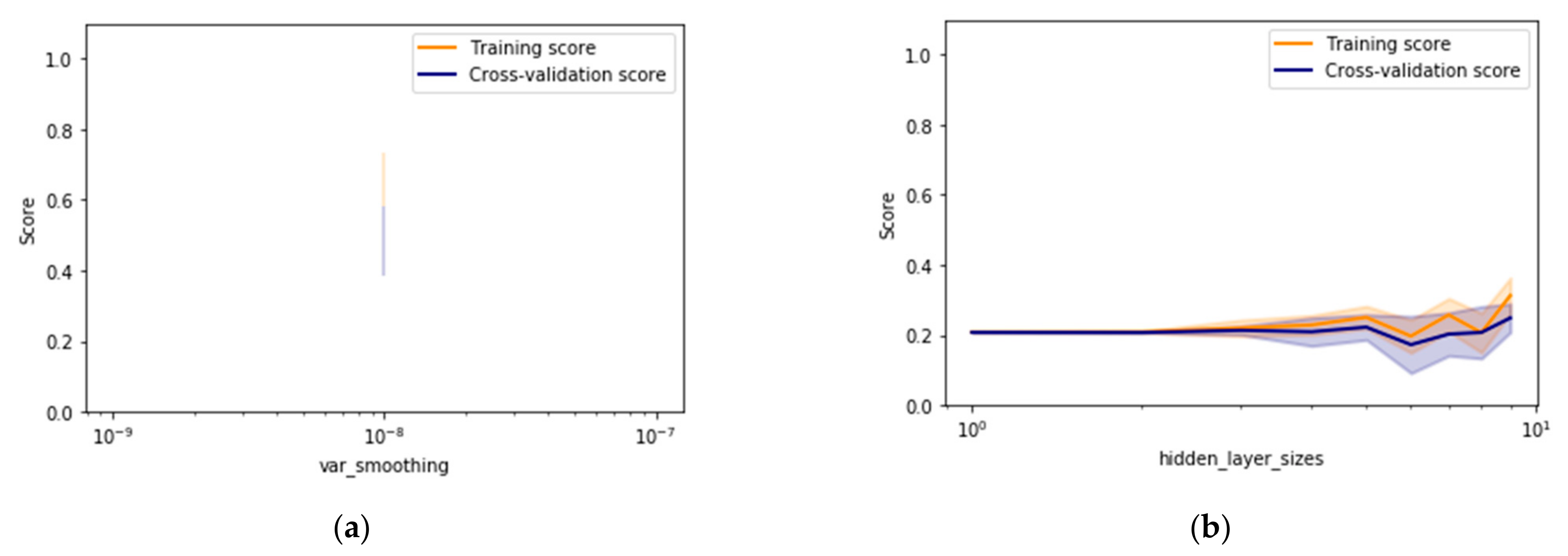
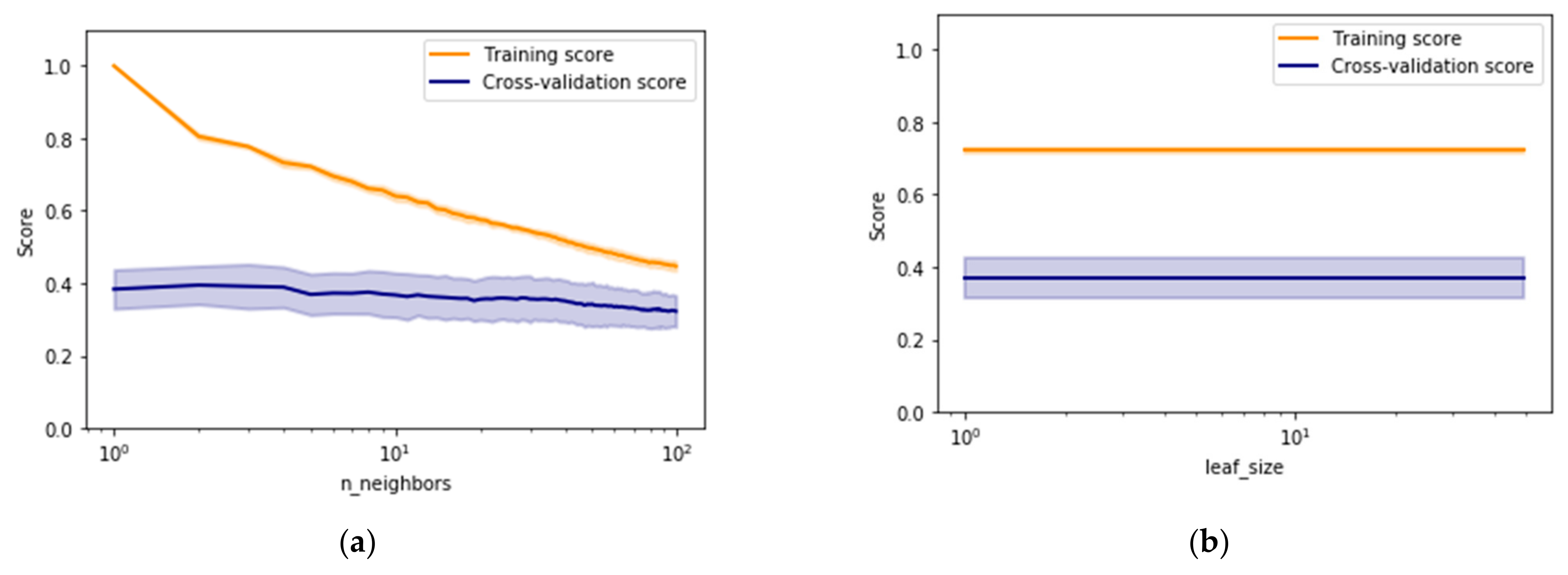
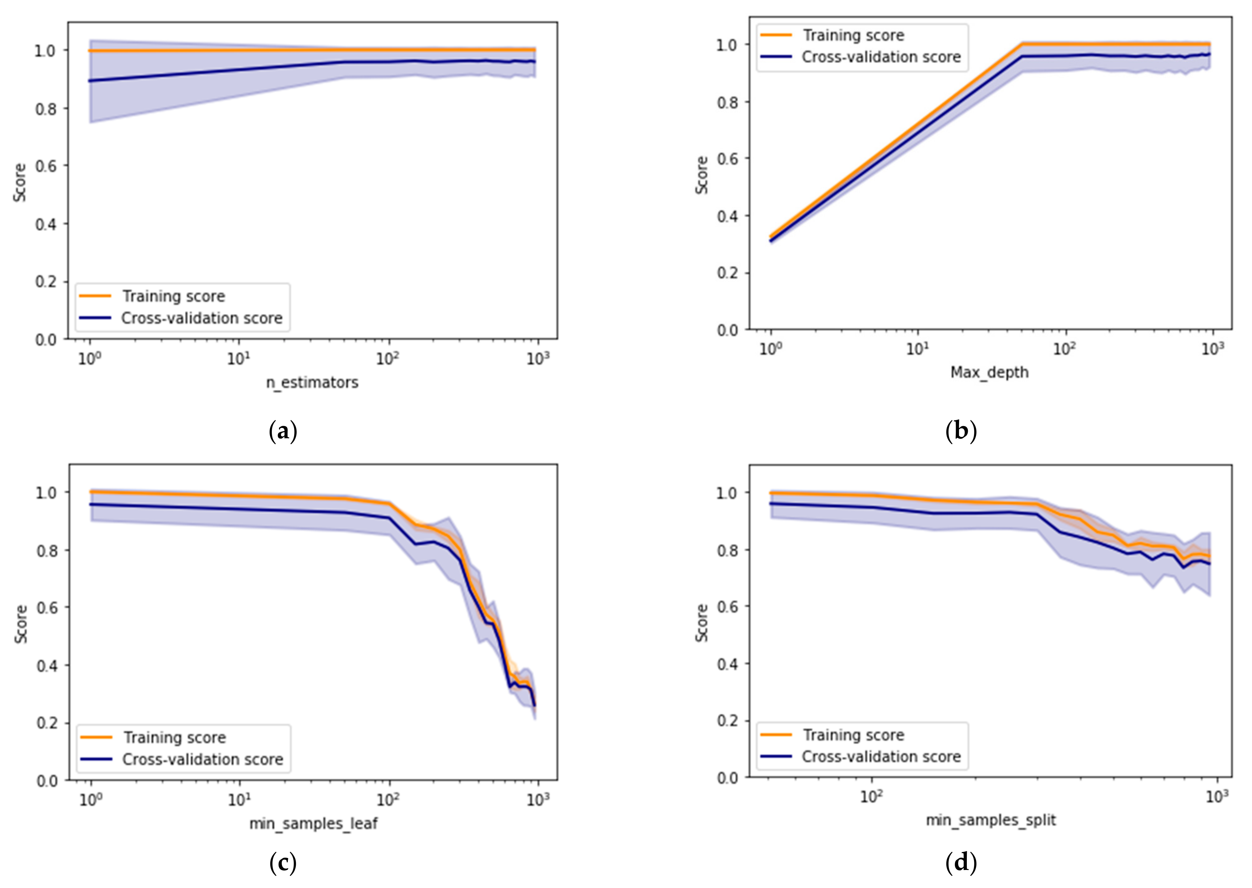
This section discusses the results obtained while selecting different types of drill bit through machine learning models. Two ensemble methods namely, AdaBoost and random forest (RF), have been investigated for handling the complex multiclass imbalanced data problem associated with the intelligent drill bit selection process. Validation curves have been generated to identify the stable regions existing in ranges of various models’ parameters as shown in Figure 7, Figure 8, Figure 9 and Figure 10. 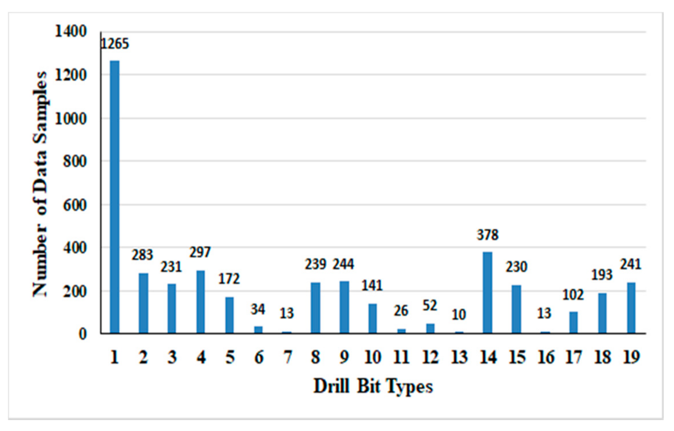A detailed description of drill bit types has been provided in Table A1 of Appendix A. Two data-driven experimental scenarios have been simulated to test the intelligent bit selection approach. In the first experimental scenario, machine learning models were trained and tested on the combined dataset obtained from eight wells using 10-FCV. The input data utilized for training and testing of various machine learning models contain uneven training samples belonging to various classes as shown in Figure 4. In the case of imbalanced data, classification accuracy becomes unreliable and unfit for the performance evaluation of machine learning models. Thus, average values of recall, precision, F1 score, G-mean, and MCC, have been determined to examine the overall performance of various machine learning models.

Table 5. The performance of machine learning classifiers for drill bit selection in the first scenario.

Classifiers	Training Accuracy	Testing Accuracy	Precision	Recall	F1score	MCC	G-Mean
NBC	56.15	55.001	0.639	0.550	0.517	0.516	0.61
KNC	63.00	60.00	0.623	0.61	0.60	0.566	0.54
MLP	72.12	71.06	0.711	0.711	0.708	0.678	0.70
SVC	0.83	0.82	0.79	0.78	0.81	0.83	0.81
AdaBoost	0.96	0.90	0.90	0.90	0.91	0.90	0.90
Random forest	0.97	0.91	0.92	0.92	0.92	0.91	0.91

shows the classification performance of standard classifiers for bit selection. It can be observed from Table 5 that the performance of NBC and KNC are the lowest among all the other classifiers. NBC has failed to learn about hidden dependencies or patterns among diverse variables present inside the training data samples related to smaller classes. Smaller classes have existed sparsely in the training data space due to data scarcity which also harms the performance of KNC with testing data.

MLP model has been trained on 70% of input data along with 15% for validation and 15% as testing data. The optimum number of the hidden layer’s neurons of MLP was estimated based on minimum training error after several iterations as shown in

Table A2. Selection of the optimum number of neurons in the hidden layer of MLP based on minimum training error.

Hidden Layer Neurons.	Neural Network	Average Percentage Error
1	15-1-19	12.95
2	15-2-19	10.724
3	15-3-19	12.1
4	15-4-19	7.42
5	15-5-19	3.97
6	15-6-19	3.26
7	15-7-19	3.6
8	15-8-19	3.44
9	15-9-19	3.09
10	15-10-19	3.88
11	15-11-19	4.59
12	15-12-19	2.91
13	15-13-19	3.67
14	15-14-19	1.55
15	15-15-19	2.91
16	15-16-19	1.85
17	15-17-19	2.38
18	15-18-19	3.53
19	15-19-19	3.03
20	15-20-19	3.83

provided in Appendix A. MLP is three layers of a popular neural network with a backpropagation (BP) paradigm in its internal architecture for the training phase. BP trains the MLP network iteratively by adjusting the weights associated with each variable present inside training data. The weights adaptation is dependent on the length of the gradient vector calculated for error minimization in the training phase. The expected length of the gradient vector is dependent on the number of samples present for each class. During imbalanced data conditions, majority classes dominate the whole error minimization process during the training phase and produce larger errors for minority classes. Thus, the performance of MLP is adversely affected by the imbalance condition. MLP, NBC, and KNC classifiers are prone to become biased for majority classes in imbalanced data conditions. However, MLP has emerged as the second-best performing single supervise classifier for drill bit selection followed by SVC in the first place as shown in Table 5. SVC is known to have some level of immunity for imbalanced data condition but become biased to majority classes in critically high imbalance condition. All of the above said supervised models fail to provide proper generalization and become unreliable for selection of drill bit type. Therefore, ensemble methods have been investigated for drill bit selection to achieve better model generalization.

AdaBoost and RF are the two ensemble methods that have been utilized for handling the imbalanced offset wells data for drill bit selection. RF has achieved higher testing accuracy than AdaBoost for bit selection as shown in Table 5. Although, ensemble methods have given much better results as compared to single supervised classifiers which are affected by the imbalance conditions. Thus, both of these techniques were modified to enhance their capability of imbalanced data classification. AdaBoost and RF have been combined with an undersampling technique that reduced the data samples from majority classes to make the whole dataset balance. Here, the class having the lowest number of data samples was taken standard (class BT 13 with 10 samples) and other classes were undersampled accordingly. However, this approach has degraded the performance of both ensemble methods as their training and testing accuracies are heavily dependent upon the majority class samples as shown in

Table 6. Modified ensemble classifiers for the classification of imbalanced drilling data.

Modified Ensembles.	Training Accuracy	Testing Accuracy	Precision	Recall	F1 Score	MCC	G-Mean
Under Sampling AdaBoost (USA)	0.95	0.74	0.80	0.70	0.75	0.88	0.89
Over sampling AdaBoost (OSA)	0.96	0.85	0.82	0.80	0.87	0.90	0.90
Under sampling RF (USRF)	0.80	0.77	0.70	0.60	0.64	0.70	0.72
Over sampling RF (OSRF)	0.89	0.87	0.83	0.68	0.86	0.89	0.91
Weighted Class RF (WCRF)	0.93	0.92	0.93	0.92	0.92	0.92	0.96
Weighted Bootstrap Class RF (WBCRF)	0.93	0.93	0.93	0.92	0.92	0.92	0.97

. In imbalanced data conditions, classifiers normally ignore smaller classes as fewer data samples are available during the training phase. It increases difficulties for intelligent paradigms to learn and identify any hidden pattern. This technique may produce satisfactory results when a reasonable amount of data samples are present in the smaller classes. Further, oversampling was performed to tackle this critical imbalance condition through SMOTE techniques. In SMOTE, the class having the largest number of data samples (BT 1 with 1265 data samples) was taken as a standard for the generation of synthetic data. SMOTE utilizes k-nearest neighbors samples (k = 5) to acquire the data distribution of subsets for each class. The results are shown in Table 6. Which demonstrate enhancement in training and testing accuracies of ensemble classifiers, along with other performance metrics for oversampling. MCC and G-mean values have also shown enhancement as compared to the earlier undersampling case. In oversampling combinations, the ensemble classifiers are found to be more reliable and stable due to the higher values of MCC and G-mean.

In the second approach, classes are assigned weights to focus the classification operation on the samples of minority classes at the algorithm level. The weights will be adjusted according to the inverse relationship with class frequencies in the training data. This will result in the formation of a weighted class RF classifier (WCRF) for the classification of imbalanced data. It can be observed from Table 6 that the WCRF has given a better performance than standard RF for drill bit selection in terms of precision, recall, MCC, and G-mean. This indicates that WCRF has a greater generalization ability than standard RF due to enhancement in testing results. The generalization of supervised models such as ANN, AdaBoost, RF, etc. depends upon their classification performance with unseen data samples that are available in testing datasets. The higher performance of the classifier with the test dataset indicates better generalization of the trained classifier model which is always desirable.

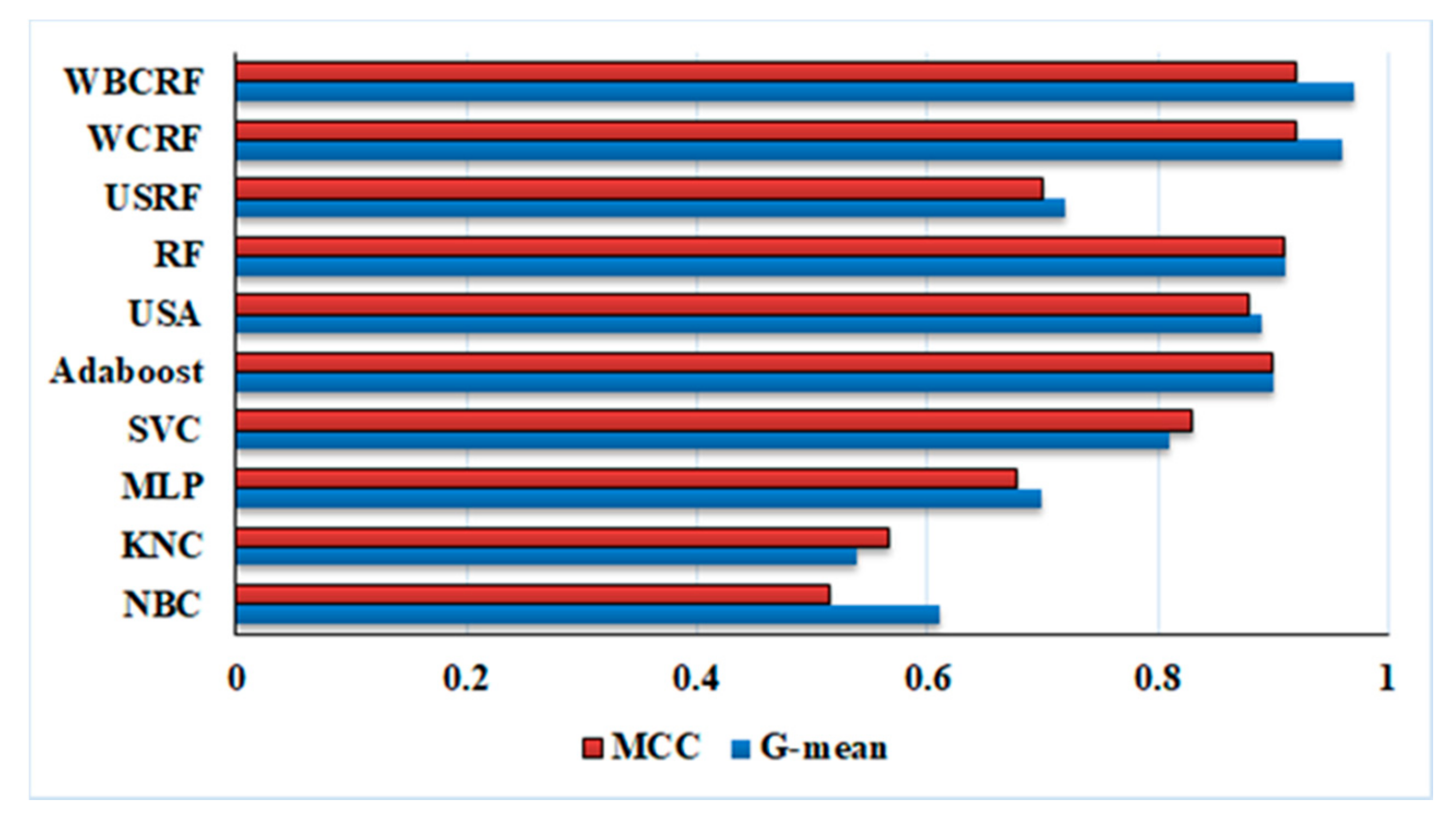
In the third approach, separate weight adjustment of classes has been performed based on its distribution in every bootstrap sample in place of the whole training dataset. Such a configuration of RF is known as RF with a bootstrap class weighting (WBCRF) classifier. This classifier contains the benefits of both data sampling and weighting techniques that are quite useful for compensating for the impact of imbalance conditions. Training and testing results of WBCRF have shown a slight performance improvement when compared with WCRF. Both these approaches have provided higher MCC and G-mean values than the standard RF paradigm as shown in Table 6 and Figure 13. The WBCRF technique has given the best classification results as compared to other classifiers considered in this study.

In the second experimental scenario, three subsets have been created from eight wells data containing data samples belonging to 17.5”, 12.25”, and 8.5” individual wellbore sections. All the earlier applied classifiers have been trained and tested on these subsets. The performance of conventional classifiers has been assessed in terms of recall, G-mean, precision, and F1 score for every BT to understand the effect of imbalanced data.

Table 7. The screening of 17.5” bits through RF and WBCRF models.

RF				WBCRF
Bit Type	Precision	Recall	F1 Score	Bit Type	Precision	Recall	F1 Score
1	1.00	1.00	1.00	1	1.00	1.00	1.00
9	0.99	1.00	0.99	9	1.00	1.00	1.00
15	0.96	1.00	0.98	15	0.96	1.00	0.98
16	1.00	0.40	0.57	16	1.00	0.70	0.71
19	1.00	0.99	0.97	19	1.00	1.00	0.99
Average	0.99	0.88	0.91	Average	0.99	0.94	0.93
Accuracy	0.98	G-mean	0.83	Accuracy	0.99	G-mean	0.85

,

Table 8. The screening of 17.5” bits through KNC and NBC models.

KNC				NBC
Bit Type	Precision	Recall	F1 Score	Bit Type	Precision	Recall	F1 Score
1	0.98	0.93	0.96	1	0.99	0.77	0.87
9	0.68	0.63	0.65	9	0.60	0.60	0.60
15	0.67	0.92	0.92	15	0.47	0.86	0.61
16	0.00	0.00	0.00	16	0.50	1.00	0.67
19	0.57	0.56	0.56	19	0.77	0.72	0.74
Average	0.58	0.61	0.59	Average	0.67	0.79	0.70
Accuracy	0.81	G-mean	00	Accuracy	0.75	G-mean	0.779

and

Table 9. The screening of 17.5” bits through MLP and SVC models.

SVC				MLP
Bit Type	Precision	Recall	F1 Score	Bit Type	Precision	Recall	F1 Score
1	1.00	0.98	0.99	1	0.99	0.95	0.97
9	0.91	0.74	0.82	9	0.79	0.81	0.80
15	0.86	0.98	0.92	15	0.80	0.98	0.88
16	0.0	0.0	0.0	16	0.00	0.00	0.00
19	0.79	0.94	0.86	19	0.83	0.80	0.81
Average	0.71	0.73	0.72	Average	0.68	0.71	0.69
Accuracy	0.92	G-mean	0.00	Accuracy	89	G-mean	0.00

contain drill bit selection test results for the 17.5” section subset. It can be observed from the abovementioned tables that bit type 16 (minority class) is hard to predict due to a smaller quantity of data points available during the training phase. KNC, SVC, and MLP have also failed to identify BT 16 due to scarcity of data samples as shown in Table 7, Table 8 and Table 9. Thus, G-mean values are recorded to be zero for SVC, KNC, and MLP as it is clear identification of the development of unreliable biased majority class classifiers.

The drill bit 16 is intentionally discussed for understanding the effects of data imbalance arise while drilling through the thin lithofacies layer. The subsurface formations have varied thickness patterns in their natural state which result in random unequal data samples for the training phase. Therefore, the uneven distribution of training data has been particularly considered to evaluate the worst to the best performance of each classifier. Uneven data samples for various bit types (class labels) in training data make classification difficult for machine learning models. Drill bit selection has been formulated as a multiclass classification problem with 19 diverse bit types as class labels as shown in Table A1. However, large fluctuation in the values of precision, recall, F1 score can be observed from Table 8 and Table 9. Standard RF has shown good classification performance even for bit type 16 due to the presence of random bootstrap resampling technique in its internal architecture. RF has given the best prediction performance for the 17.5” section subset with good immunity to data imbalance conditions. Further, WBCRF has also been evaluated for 17.5” datasets that have given more accurate results with stable values for precision, recall, and F1 score.

In the data subset of the 12.25” section, performance for every classifier has been recorded as shown in

Table 10. The screening of 12.25” bits through RF and WBCRF models.

RF				WBCRF
Bit Type	Precision	Recall	F1 Score	Bit Type	Precision	Recall	F1 Score
2	0.96	0.98	0.97	2	0.96	0.99	0.97
4	0.99	0.96	0.97	4	0.98	0.96	0.97
6	0.86	0.86	0.86	6	1.00	0.71	0.83
10	0.79	0.81	0.80	10	0.80	0.86	0.83
11	0.80	0.57	0.67	11	1.00	0.73	0.72
17	0.75	0.80	0.77	17	0.78	0.83	0.81
Average	0.86	0.83	0.84	Average	0.92	0.85	0.86
Accuracy	0.91	G-mean	0.82	Accuracy	0.92	G-mean	0.84

,

Table 11. The screening of 12.25” bit through KNC and NBC models.

KNC				NBC
Bit Type	Precision	Recall	F1 Score	Bit Type	Precision	Recall	F1 Score
2	0.80	0.84	0.82	2	0.73	0.44	0.55
4	0.78	0.86	0.81	4	0.69	0.56	0.62
6	0.62	0.71	0.67	6	0.67	0.86	0.75
10	0.85	0.79	0.81	10	0.38	0.60	0.46
11	1.00	0.43	0.60	11	0.22	0.86	0.35
17	0.78	0.60	0.68	17	0.38	0.47	0.42
Average	0.81	0.70	0.73	Average	0.51	0.63	0.52
Accuracy	0.79	G-mean	0.685	Accuracy	0.53	G-mean	0.60

and

Table 12. The screening of 12.25” bits through SVC and MLP classifier.

SVC				MLP
Bit Type	Precision	Recall	F1 Score	Bit Type	Precision	Recall	F1 Score
2	0.98	0.98	0.98	2	0.81	0.85	0.83
4	1.00	0.99	0.99	4	0.77	0.94	0.85
6	0.86	0.86	0.86	6	0.75	0.43	0.55
10	0.94	0.74	0.83	10	0.79	0.81	0.80
11	0.75	0.86	0.80	11	0.00	0.00	0.00
17	0.74	0.97	0.84	17	0.93	0.43	0.59
Average	0.88	0.90	0.88	Average	0.67	0.58	0.79
Accuracy	0.94	G-mean	0.80	Accuracy	0.79	G-mean	0.00

. Higher fluctuations in the values of precision, recall, and F1 score has been recorded in classification results. This indicates that these sections are physically challenging drilling zones. RF and WBCRF have given impressive results for the classification of these critical geological zones as shown in Table 10, Table 11 and Table 12. In this section, BTs 6 and 11 are minority classes that are hard to classify. However, only MLP becomes a bias classifier as it fails to classify any samples for BT 11 as shown in Figure 13.

The geological lithofacies existing in section 8.5” are found to be the most challenging formations for drilling operations due to several faults and unstable zones existing along its depths. The 8.5” section formations have been reported to be unstable because they are made up of softer rocks such as claystone, sandstone, siltstone, tuff, marl, limestone, and argillaceous clay contents. Certain incidents of gas leaks and drill string stuck ups were also recorded while drilling 8.5” section of the wells with high stick slips conditions in its upper formations. Polycrystalline diamond compact bits (PDC) were primarily utilized for drilling softer 8.5” section because of their higher ROP values and stable drilling operation (Table A1). However, it becomes difficult for the driller to choose the right PDC bit type as varieties of bit models are available while planning for drilling operations. The pattern recognition has become difficult in the 8.5” section as the performance of all the classifiers has shown more fluctuations in their precision and recall values due to heterogeneity of lithofacies as shown in

Table 13. The selection of 8.5” bits through RF and WBCRF models.

RF				WBCRF
Bit Type	Precision	Recall	F1 Score	Bit Type	Precision	Recall	F1 Score
3	0.91	0.99	0.95	3	0.92	0.99	0.95
5	0.98	0.87	0.92	5	0.98	0.89	0.93
12	0.93	0.81	0.87	12	0.93	0.81	0.87
13	1.00	0.67	0.80	13	1.00	1.00	1.00
18	0.89	0.98	0.93	18	0.94	0.98	0.96
Average	0.94	0.86	0.93	Average	0.95	0.93	0.94
Accuracy	0.93	G-mean	0.855	Accuracy	0.94	G-mean	0.931

,

Table 14. The selection of 8.5” drill bits through KNC and NBC models.

KNC				NBC
Bit Type	Precision	Recall	F1 Score	Bit Type	Precision	Recall	F1 Score
3	0.74	0.92	0.82	3	0.71	0.93	0.80
5	0.52	0.42	0.46	5	0.80	0.51	0.62
12	0.24	0.25	0.24	12	0.39	0.69	0.50
13	0.00	0.00	0.00	13	0.43	0.33	0.38
18	0.60	0.61	0.60	18	0.74	0.57	0.64
Average	0.42	0.44	0.43	Average	0.61	0.61	0.59
Accuracy	0.61	G-mean	0.00	Accuracy	0.68	G-mean	0.573

and

Table 15. The selection of 8.5” bits through SVC and MLP classifiers.

SVC				MLP
Bit Type	Precision	Recall	F1 Score	Bit Type	Precision	Recall	F1 Score
3	1.00	0.99	0.99	3	0.79	1.00	0.88
5	0.96	0.84	0.89	5	0.90	0.49	0.64
12	0.77	0.62	0.62	12	0.57	0.50	0.53
13	0.67	0.22	0.33	13	0.00	0.00	0.00
18	0.72	0.96	0.82	18	0.65	0.86	0.74
Average	0.82	0.73	0.75	Average	0.58	0.57	0.56
Accuracy	0.88	G-mean	0.643	Accuracy	0.74	G-mean	0.00

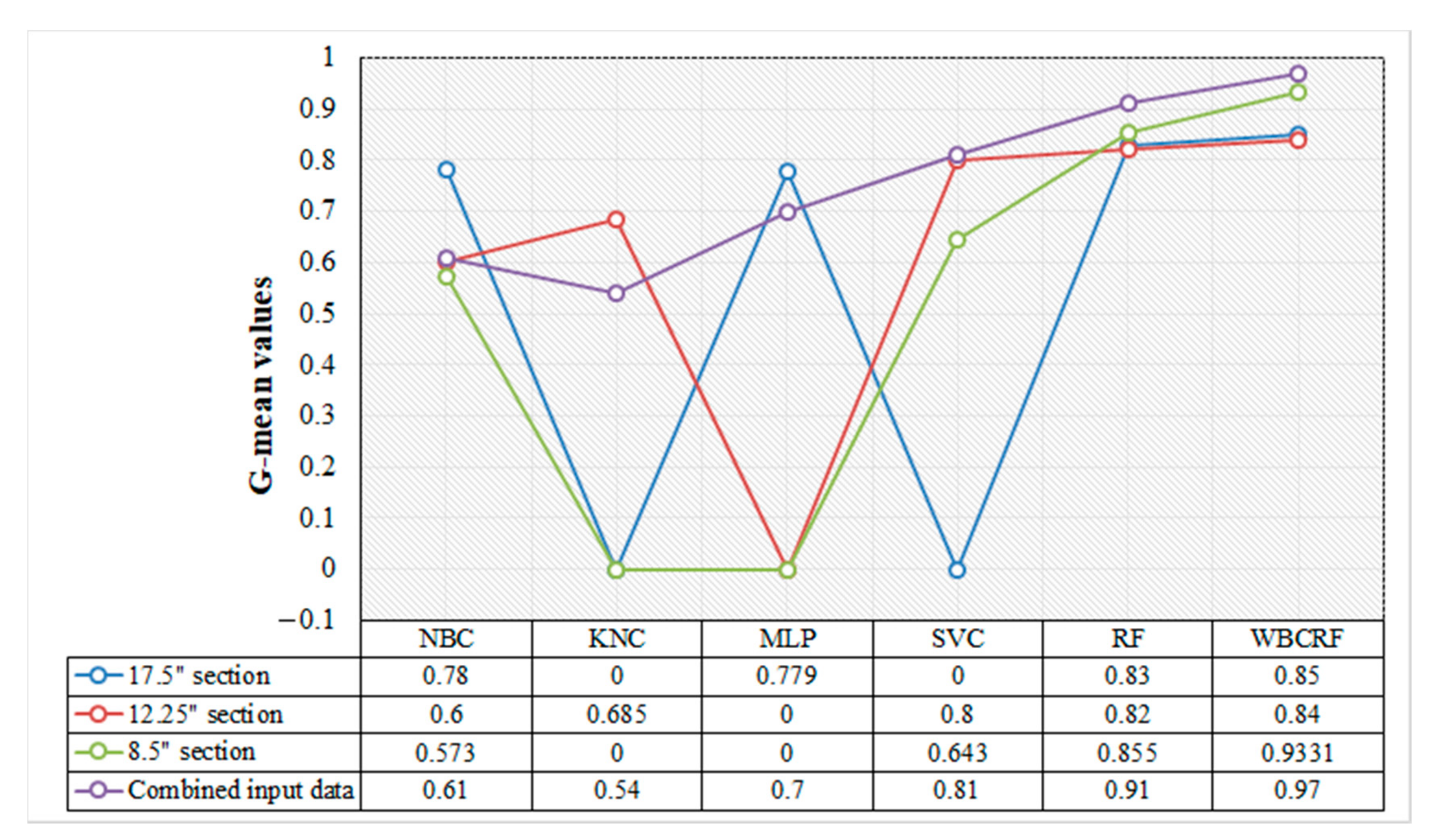
. Here, BT 12 and 13 are the minority classes for which KNC and MLP failed to identify any samples while SVC and NBC have shown poor prediction performance as shown in Figure 13. Finally, worst-to-best accuracy of various classifiers in second data-driven scenario can be given as: WBCRF (0.92–0.99), RF (0.91–0.98), SVC (0.88–0.94), MLP (0.74–0.89), KNC (0.61–0.81), and NBC (0.53–0.75). RF and WBCRF have shown great immunity for data imbalance condition and successfully maintained their performance even in the critical 8.5” section. Recently, hybrid drill bits (e.g., Kymera) have been developed that combined the properties of conventional PDC bit and roller cone bit types [56]. These hybrid bits seem to be a good solution for drilling problematic 8.5” section while maintaining the stability of drilling operations. Figure 14 provides a summary of G-mean scores achieved by intelligent models for both experimental scenarios. A comparative table of significant research publications has been provided in Appendix A as

Table A3. A comparative study of significant methods applied for drill bit selection.

S. No.	Publication	Techniques	Field Details	Data Types	Advantages	Limitations
1.	Rabia (1985) [6]	Cost per foot	Unavailable	Operational drilling parameters	Simple to apply and empirical in nature	Unfit for horizontal and multilateral drilling operation and low accuracy
2.	Rabia et al. (1986) [5]	Specific Energy	Southern North Sea	Operational drilling parameters	Simple to apply	Based on only three operational parameter and low accuracy
4.	Hightower, (1964) [8]	Offset Well logs	County of East Texas	Well logs	Easy application	Indirect measurement of rock properties with high chances of error risk
5.	Perrin et al. (1997) [10]	drilling index	Unavailable	Operational drilling parameters	empirical correlation and can be easily applied	Low accuracy and high chances of error
6.	Xu et al. (1997) [12]	Empirical modeling	Unavailable	Mud logging data, operational drilling data	Improved cost per foot model	Mathematically complex and requires more data
7.	Mensa-Wilmot et al. (1999) [11]	Formation drillability parameter	Unavailable	Rock mechanical and geologic properties	Indirect measurements, and more accurate then empirical correlations	High level of uncertainty in well logs data due to hydrocarbon reservoir heterogeneity
10.	Uboldi et al. (1999) [13]	Rock strength measurements and indentation technique	Southern Italy, near Apennines chain	Rock mechanical and geologic properties	Accurate measurement of core properties	Require testing lab, costly and time-consuming
11.	Bilgesu et al. (2000) [2]	ANN	Middle East field	BS, WOB, RPM, pump rate, DT, and BT	High prediction accuracy	Not immune to imbalanced data, noise, overfitting and underfitting problems
12.	Yιlmaz, et al. (2002) [17]	ANN and fractal geostatistics	southeast Turkey.	rock bit data	High prediction accuracy	Not immune to imbalanced data, noise, overfitting and underfitting problems
13.	Bataee et al. (2010) [7]	bit dullness	Shadegan oil field	Human experience	Simple, empirical, and organized.	Requires human visual expertise with high chances of error
14.	Edalatkhah, Rasoul, and Hashemi, (2010) [18]	ANN and Genetic algorithm	South Pars Field	Drilling operational data	More accurate than individual ANN model	Not immune to imbalanced data, noise, overfitting and underfitting problems
15.	Hou, Chien, and Yuan, (2014) [19]	ANN	Tarim Oilfield,	offset wells data, drillability, and lithofacies information	More accurate then empirical models	Not immune to imbalanced data, noise, overfitting and underfitting problems
16.	Sherbeny et al. (2016) [14]	Image logs and mineralogy logs	Unavailable	Image data and mineralogy data	Accurate method	Application in limited lithofacies, computationally challenging, and costly technology.
17.	Nabilou (2016) [20]	Resistance against Drilling	Southwest of Iran	Geo-Mechanical data	More accurate than the empirical correlation	Application in limited lithofacies, computationally challenging and costly technology
18.	Mardiana and Noviasta (2017) [15]	Rock strength analysis and Dynamic Finite-Element Analysis (FEA) Modeling	Unavailable	Offset well logs data	More accurate than the empirical correlation	Application in limited lithofacies, computationally challenging and costly technology
19.	Momeni et al. (2018) [22]	ANN	Unavailable	drilling bit records from offset wells	More accurate than the empirical correlation	Not immune to imbalanced data, noise, overfitting and underfitting problems
20.	Cornel and Vazquez (2020) [16]	Rock Strength Analysis and bit dull grading approach	South West of Wandoan, Queensland	dull grading and bit records	More accurate than the empirical correlations	Application in limited lithofacies, computationally challenging and costly technology
21.	Abbas et al. (2019) [23]	ANN, Genetic algorithm and Mechanical earth model	Unavailable	Operational drilling parameters	More accurate than individual ANN model and empirical models	Not immune to imbalanced data, noise, overfitting and underfitting problems
22.	Proposed Approach	Ensemble methods and Resampling techniques	North Sea	Operational drilling parameters and mud logging data	More reliable, stable, and accurate than previous models	Need to be tested on field with streaming data conditions.

.

The present study shows that the ensemble methods have great potential for automatic drill bit selection. With data resampling and boosting approaches, reliability, stability, and performances of ensemble methods have improved as discussed in earlier parts of this section. The proposed models do not have any known specific limitation. However, these models are needed to be tested on the field with real-time streaming well data to achieve more insight about their performance in practical scenarios. With the rapid advancement in sensor based data acquisition new measurements may be available in future oil and gas wells. This will require retraining of the proposed models with newer training data sets. More research work is required for understanding the drill bit selection process with real-time streaming data. It is highly recommended that driller (field engineers) should understand the problems associated with drilling data before applying any data driven models for drill bit selection. During data acquisition, data samples must be carefully captured in such a way that equal number of data samples will be available for each geological formations. The proposed models is advancement in the existing technology that will enhance the efficiency of drilling operations for better extraction and utilization of hydrocarbon resources for long sustainable time period. This will promote global economic development that have huge impact on human sustainability. This will also satisfy the goals of sustainable development described by United Nation Development Programme (UNDP). To meet the global energy demands, more unconventional wells are being drilled that requires industrial innovation to face the technological challenges. This study provides an approach to automate the drill bit selection process over any field, which will minimize human error, time, and drilling operational costs.

6. Conclusions

A novel data-driven approach has been proposed using the fusion of data resampling technique and ensemble method for handling the imbalance issues of complex drilling data. The problem of imbalanced training data results in the development of unreliable biased classifiers that are unfit for practical field applications. Two experimental data-driven scenarios have been specially designed and tested to confirm the generalization of the proposed approach for drill bit selection. An extensive comparative study has been performed to evaluate the performance of popular classifiers for the screening of drill bits. After a meticulous comparison of results, the following important conclusions can be drawn as given below:

• WBCRF technique has given the most impressive performance during automatic bit type selection with testing accuracy ranges from 92% to 99%, and G-mean (0.84–0.97) for various experimental scenarios.
• The large fluctuations in the performance of classifiers have been recorded in the 8.5” section in terms of precision, recall, and F1 scores. It is observed that drill bit selection becomes difficult in the lower formations due to uncertainty in subsurface conditions.
• Data imbalance condition exists due to the drilling of thin lithofacies that harm the performance of classifiers.
• WBCRF has given good prediction results for screening drill bit even for critical drilling zones.
• The performance of conventional classifiers is largely affected by data imbalance issues. Conventional classifiers can’t be trusted for the drill bit selection, especially for critical drilling zones.
• RF has shown great immunity for data imbalance conditions and successfully maintained its performance even in the critical 8.5” section.
• The proposed approach can also be applied over any other oil and gas fields to automate the drill bit selection, which will minimize human error, time, and drilling cost.
• The combination of ensemble methods with the data resampling technique results in modified ensemble classifiers that are found to be efficient even in highly imbalanced conditions.

The present study shows that the ensemble methods have great potential for automatic drill bit selection. More research work is required for understanding the drill bit selection process with real-time streaming data. In future work, the reinforcement learning approach will be investigated with streaming drilling data for automatic decision making in real-time. The reinforcement learning approach seems to be quite a good option for the automation of various drilling processes as it has the potential to enhance the performance of its models in real-time conditions which is impossible for supervised paradigms.

References

1. Fear, M.J.; Meany, N.C.; Evans, J.M. An expert system for drill bit selection. In Proceedings of the SPE/IADC Drilling Conference, Dallas, TX, USA, 15–18 February 1994. [Google Scholar]
2. Bilgesu, H.I.; AL-Rashidi, A.F.; Aminian, K.; Ameri, S. A new approach for drill bit selection. In Proceedings of the SPE Eastern Regional Meeting, Morgantown, WV, USA, 17–19 October 2000. [Google Scholar]
3. Tewari, S.; Dwivedi, U.D. A Real-World Investigation of TwinSVM for the Classification of Petroleum Drilling Data. In Proceedings of the IEEE Region 10 Symposium (TENSYMP), Kolkata, India, 7–9 June 2019; pp. 90–95. [Google Scholar]
4. Chaki, S.; Routray, A.; Mohanty, W.K.; Jenamani, M. A novel multiclass SVM based framework to classify lithology from well logs: A real-world application. In Proceedings of the Annual IEEE India conference (INDICON), New Delhi, India, 17–20 December 2015; pp. 2325–9418. [Google Scholar]
5. Rabia, H.; Farrelly, M.; Barr, M.V. A new approach to drill bit selection. In Proceedings of the European Petroleum Conference, London, UK, 20–22 October 1986. [Google Scholar]
6. Rabia, H. Specific Energy as a Criterion for Bit Selection. J. Pet. Technol. 1985, 37, 1225–1229. [Google Scholar] [CrossRef]
7. Bataee, M.; Edalatkhah, S.; Ashena, R. Comparison between bit optimization using artificial neural network and other methods base on log analysis applied in Shadegan oil field. In Proceedings of the International Oil and Gas Conference and Exhibition in China, Beijing, China, 8–10 June 2010. [Google Scholar]
8. Hightower, W.J. Proper selection of drill bits and their use. In Proceedings of the SPE Mechanical Engineering Aspects of Drilling and Production Symposium, Fort Worth, TX, USA, 23–24 March 1964. [Google Scholar]
9. Mason, K.L. Three-Cone Bit Selection with Sonic Logs. SPE Drill. Eng. 1987, 2, 135–142. [Google Scholar] [CrossRef]
10. Perrin, V.P.; Wilmot, M.G.; Alexander, W.L. Drilling index-a new approach to bit performance evaluation. In Proceedings of the S.P.E./I.A.D.C. Drilling Conference, Amsterdam, The Netherlands, 4–6 March 1997; pp. 199–205. [Google Scholar]
11. Mensa-Wilmot, G.; Calhoun, B.; Perrin, V.P. Formation drillability-definition, quantification and contributions to bit performance evaluation. In Proceedings of the SPE/ IADC Middle East Drilling Technology Conference, Abu Dhabi, UAE, 8–10 November 1999. [Google Scholar]
12. Xu, H.; Tochikawa, T.; Hatakeyama, T. A practical method for modeling bit performance using mud logging data. In Proceedings of the S.P.E./I.A.D.C. Drilling Conference, Amsterdam, The Netherlands, 4–6 March 1997; pp. 127–131. [Google Scholar]
13. Uboldi, V.; Civolani, L.; Zausa, F. Rock strength measurements on cuttings as input data for optimizing drill bit selection. In Proceedings of the SPE Annual Technical Conference and Exhibition, Houston, TX, USA, 3–6 October 1999. [Google Scholar]
14. Sherbeny, W.E.; Hasan, G.; Lindsay, B.W.; Madkour, A.; Nagy, A.; Abulawi, M.; Mohammad, M.S.; Richard, A. Role of wellbore imaging and specific mineralogy inputs data in bit selection and design software. In Proceedings of the SPE Kingdom of Saudi Arabia Annual Technical Symposium and Exhibition, Dammam, Saudi Arabia, 25–28 April 2016. [Google Scholar]
15. Mardiana, M.R.; Noviasta, B. Rock strength analysis and integrated FEM modeling optimise bit selection for deepwater exploration. In Proceedings of the SPE/IATMI Asia Pacific Oil & Gas Conference and Exhibition, Jakarta, Indonesia, 17–19 October 2017. [Google Scholar]
16. Cornel, S.; Vazquez, G. Use of big data and machine learning to optimise operational performance and drill bit design. In Proceedings of the SPE Asia Pacific Oil & Gas Conference and Exhibition, Perth, Australia, 20–22 October 2020. [Google Scholar]
17. Yιlmaz, S.; Demircioglu, C.; Akin, S. Application of artificial neural networks to optimum bit selection. Comput. Geosci. 2002, 28, 261–269. [Google Scholar] [CrossRef]
18. Edalatkhah, S.; Rasoul, R.; Hashemi, A. Bit selection optimization using artificial intelligence systems. Pet. Sci. Technol. 2010, 28, 1946–1956. [Google Scholar] [CrossRef]
19. Hou, B.; Chen, M.; Yuan, J. Optimization and Application of Bit Selection Technology for Improving the Penetration Rate. Res. J. Appl. Sci. Eng. Technol. 2014, 8, 179–187. [Google Scholar] [CrossRef]
20. Nabilou, A. Effect of Parameters of Selection and Replacement Drilling Bits Based on Geo-Mechanical Factors: (Case Study: Gas and Oil Reservoir in the Southwest of Iran). Am. J. Eng. Appl. Sci. 2016, 9, 380–395. [Google Scholar] [CrossRef] [Green Version]
21. Efendiyev, G.M.; Mammadov, P.Z.; Piriverdiyev, I.A.; Sarbopeyeva, M.D. Selection of the best combination of bit types and technological parameters during drilling, taking into account uncertainty. Procedia Comput. Sci. 2017, 120, 67–74. [Google Scholar] [CrossRef]
22. Momeni, M.S.; Ridha, S.; Hosseini, S.J.; Meyghani, B.; Emamian, S.S. Bit selection using field drilling data and mathematical investigation. In IOP Conference Series: Materials Science and Engineering; Institute of Physics Publishing: Bristol, UK, 2018; p. 012008. [Google Scholar]
23. Abbas, A.K.; Assi, A.H.; Abbas, H.; Almubarak, H.; Saba, M.A. Drill bit selection optimization based on rate of penetration: Application of artificial neural networks and Genetic algorithm. In Proceedings of the SPE Abu Dhabi International Exhibition and Conference, UAE, Abu Dhabi, 11–14 November 2019. [Google Scholar]
24. Manuel, Y.A.; Momeni, M.; Hamdi, Z.; Zivar, D. A new method of bit selection using drill bit images. In Proceedings of the Offshore Technology Conference Asia, Malaysia, Kuala Lumpur, 2 November 2020. [Google Scholar]
25. Longadge, R.; Dongre, S. Class imbalance problem in data mining review. arXiv 2013, arXiv:1305.1707. Available online: http://arxiv.org/abs/1305.1707 (accessed on 16 August 2019).
26. Ghorbani, R.; Ghousi, R. Comparing Different Resampling Methods in Predicting Students’ Performance Using Machine Learning Techniques. IEEE Access 2020, 8, 67899–67911. [Google Scholar]
27. Chawla, N.V.; Bowyer, K.W.; Hall, L.O.; Kegelmeyer, W.P. SMOTE: Synthetic Minority Over-sampling Technique. J. Artif. Intell. Res. 2002, 16, 321–357. [Google Scholar]
28. Lhassan, T.; Aljurf, M.; Al-Mohanna, F.; Shoukri, M. Classification of Imbalance Data using Tomek Link (T-Link) Combined with Random Under-sampling (RUS) as a Data Reduction Method. J. Inform. Data Min. 2016, 1, 1–11. [Google Scholar]
29. Polikar, R. Ensemble-Based Systems in Decision Making. IEEE Circuits Syst. Mag. 2006, 6, 21–45. [Google Scholar] [CrossRef]
30. Zang, C.; Ma, Y. Ensemble Machine Learning: Methods and Application; Springer Publication: New York, NY, USA, 2012. [Google Scholar]
31. Freund, Y.; Schapire, R.E. Experiments with a new boosting algorithm. In Proceedings of the Machine learning: Thirteenth International Conference, Bari, Italy, 3–6 July 1996; pp. 148–156. [Google Scholar]
32. Sun, Y.; Wong, A.K.C.; Kamel, M.S. Classification of imbalanced data: A review. Int. J. Pattern Recognit. Artif. Intell. 2009, 23, 687–719. [Google Scholar] [CrossRef]
33. Breiman, L. Random forests. Mach. Learn. 2001, 45, 5–32. [Google Scholar]
34. Cutler, A.; Cutler, D.R.; Stevens, J.R. Random forests. In Ensemble Machine Learning, 2nd ed.; Zhang, C., Ma, Y.Q., Eds.; Springer: New York, NY, USA, 2012; pp. 157–175. [Google Scholar]
35. Ho, T.K. Random decision forests. In Proceedings of the 3rd International conference on document analysis and recognition, Montreal, QC, Canada, 14–16 August 1995. [Google Scholar]
36. Chen, C.; Liaw, A.; Bremain, L. Using Random Forest to Learn Imbalanced Data. Report Number 666. 2004. Available online: https://statistics.berkeley.edu/sites/default/files/tech-reports/666.pdf (accessed on 1 November 2020).
37. Cover, T.; Hart, P. Nearest neighbor pattern classification. IEEE Trans. Inf. Theory 1967, 13, 21–27. [Google Scholar] [CrossRef]
38. McCallum, A.; Nigam, K. A comparison of event models for naive bayes text classification. In Proceedings of the AAAI’98 Workshop on Learning for Text Categorization. AAAI Digital Library, Madison, WI, USA, 26–27 July 1948; pp. 41–48. [Google Scholar]
39. Balaji, V.R.; Suganthi, S.T.; Rajadevi, R.; Kumar, V.K.; Balaji, B.S.; Pandiyan, S. Skin disease detection and segmentation using dynamic graph cut algorithm and classification through Naive Bayes Classifier. Measurement 2020, 163, 107922. [Google Scholar]
40. Haykin, S. Neural Networks, a Comprehensive Foundation; Prentice Hall PTR: Upper Saddle River, NJ, USA, 1998. [Google Scholar]
41. Vapnik, V. The Nature of Statistical Learning; Springer: New York, NY, USA, 2000. [Google Scholar]
42. Cortes, C.; Vapnik, V. Support-vector networks. Mach. Learn. 1995, 20, 273–297. [Google Scholar]
43. Equinor Website Database. Available online: https://www.equinor.com/en/how-and-why/digitalisation-in-our-dna/volve-field-data-village-download.html (accessed on 17 August 2020).
44. Gan, C.; Cao, W.; Wu, M.; Liu, K.; Chen, X.; Hu, Y.; Ning, F. Two-level intelligent modeling method for the rate of penetration in complex geological drilling process. Appl. Soft Comput. 2019, 80, 592–602. [Google Scholar]
45. Løken, E.A.; Løkkevik, J.; Sui, D. Data-driven approaches tests on a laboratory drilling system. J. Pet. Explor. Prod. Technol. 2020, 10, 3043–3055. [Google Scholar]
46. Karadzhova, G.N. Drilling Efficiency and Stability Comparison between Tricone, PDC and Kymera Drill Bits. Master’s Thesis, University of Stavanger, Stavanger, Norway, 2014. [Google Scholar]
47. Akisanmi, O.A. Automatic Management of Rate of Penetration in Heterogeneous Formation Rocks. Master’s Thesis, University of Stavanger, Stavanger, Norway, 2016. [Google Scholar]
48. Kenneth, E.; Russel, S.C. Innovative ability to change drilling responses of a PDC bit at the rig site using interchangeable depth of-cut control features. In Proceedings of the IADC/SPE Drilling Conference and Exhibition, Fort Worth, TX, USA, 1–3 March 2016. [Google Scholar]
49. Jayadeva, J.; Kumar, D.; Naik, G.R. TwinSVM gesture classification using the surface Electromyogram. IEEE Trans. Inf. Technol. Biomed. 2010, 14, 301–308. [Google Scholar]
50. Diaz, M.B.; Kim, K.Y.; Kang, T.H.; Shin, H.S. Drilling data from an enhanced geothermal project and its pre-processing ROP forecasting improvement. Geothermics 2018, 72, 348–357. [Google Scholar] [CrossRef]
51. Mustaffa, Z.; Yusof, Y. A comparison of normalization techniques in predicting dengue outbreak. In Proceedings of the International Conference on Business and Economics Research, Kuala Lumpur, Malaysia, 26–28 November 2010. [Google Scholar]
52. Tewari, S.; Dwivedi, U.D. A comparative study of heterogeneous ensemble methods for the identification of geological lithofacies. J. Pet. Explor. Prod. Technol. 2020, 10, 1849–1868. [Google Scholar] [CrossRef] [Green Version]
53. Gan, C.; Cao, W.H.; Wu, M.; Chen, X.; Hu, Y.L.; Liu, K.Z.; Wang, F.W.; Zhang, S.B. Prediction of drilling rate of penetration (ROP) using hybrid support vector regression: A case study on the Shennongjia area, Central China. J. Pet. Sci. Eng. 2019, 181, 1060200. [Google Scholar] [CrossRef]
54. Kohavi, R. A study of cross validation and bootstrap for accuracy estimation and model selection. In Proceedings of the 14th International Joint Conference Artificial Intelligence, San Francisco, CA, USA, 20–25 August 1995; pp. 1137–1143. [Google Scholar]
55. Kubat, M.; Holte, R.; Matwin, S. Learning when negative examples abound. In Proceedings of the 9th European Conference on Machine Learning, Berlin/Heidelberg, Germany, 23–25 April 1995; Springer: London, UK, 1995; pp. 146–153. [Google Scholar]
56. Pessier, R.; Damschen, M. Hybrid bits offer distinct advantages in selected roller-cone and pdc-bit applications. SPE Drill. Complet. 2011, 26, 96–103. [Google Scholar] [CrossRef]
Figure 1. A generalized workflow of the AdaBoost algorithm.
Energies 14 00432 g001
Figure 2. A generalized workflow of the Random Forest algorithm.
Energies 14 00432 g002
Figure 3. Geological location of Volve oil and gas field (courtesy: Equinor website) [43].
Energies 14 00432 g003
Figure 4. The number of data samples available in real field drilling data for each bit type.
Energies 14 00432 g004
Figure 5. The denoising of WOB variable using the 1-D Wavelet filtering technique.
Energies 14 00432 g005
Figure 6. Importance of input drilling variables for the selection of drill bit type.
Energies 14 00432 g006
Figure 7. Validation curves generated for NBC and MLP (a) NBC Smoothing parameter and (b) MLP number of hidden layers.
Energies 14 00432 g007
Figure 8. Validation curves generated for the important parameters of KNC classifier (a) Number of neighbors (b) Leaf size.
Energies 14 00432 g008
Figure 9. Validation curves generated for two important parameters of SVC classifier (a) Regularization parameter C (b) Gamma parameter.
Energies 14 00432 g009
Figure 10. Validation curves generated for four important parameters of RF (a) Number of estimators (b) Maximum depth of decision tree (c) Minimum samples needed at leaf node (d) Minimum number of samples needed for splitting.
Energies 14 00432 g010
Figure 11. Minimization of classification error plot generated during the training phase of SVC using the Grid search technique.
Energies 14 00432 g011
Figure 12. A generalized workflow of drill bit selection process based on the proposed approach.
Energies 14 00432 g012
Figure 13. MCC and G-mean scores of machine learning models considered in this study for the first experimental scenario.
Energies 14 00432 g013
Figure 14. Summary of G-mean scores achieved by intelligent models for both experimental scenarios.
Energies 14 00432 g014