Article

Adaptive Surrogate Estimation with Spatial Features Using a Deep Convolutional Autoencoder for CO2 Geological Sequestration

1
Geo-ICT Convergence Research Team, Korea Institute of Geoscience and Mineral Resources, Daejeon 34132, Korea
2
Department of Energy and Resources Engineering, Kangwon National University, Chuncheon 24341, Korea
*
Author to whom correspondence should be addressed.
Energies 2021, 14(2), 413; https://doi.org/10.3390/en14020413
Submission received: 26 November 2020 / Revised: 2 January 2021 / Accepted: 10 January 2021 / Published: 13 January 2021

Abstract

:
This paper develops a reliable deep-learning framework to extract latent features from spatial properties and investigates adaptive surrogate estimation to sequester CO2 into heterogeneous deep saline aquifers. Our deep-learning architecture includes a deep convolutional autoencoder (DCAE) and a fully-convolutional network to not only reduce computational costs but also to extract dimensionality-reduced features to conserve spatial characteristics. The workflow integrates two different spatial properties within a single convolutional system, and it also achieves accurate reconstruction performance. This approach significantly reduces the number of parameters to 4.3% of the original number required, e.g., the number of three-dimensional spatial properties needed decreases from 44,460 to 1920. The successful dimensionality reduction is accomplished by the DCAE system regarding all inputs as image channels from the initial stage of learning using the fully-convolutional network instead of fully-connected layers. The DCAE reconstructs spatial parameters such as permeability and porosity while conserving their statistical values, i.e., their mean and standard deviation, achieving R-squared values of over 0.972 with a mean absolute percentage error of their mean values of less than 1.79%. The adaptive surrogate model using the latent features extracted by DCAE, well operations, and modeling parameters is able to accurately estimate CO2 sequestration performances. The model shows R-squared values of over 0.892 for testing data not used in training and validation. The DCAE-based surrogate estimation exploits the reliable integration of various spatial data within the fully-convolutional network and allows us to evaluate flow behavior occurring in a subsurface domain.

1. Introduction

Data science has revolutionized engineering analytics in the oil and gas industry. Data-driven analyses are now assisting the decision-making process making it more reliable as well as more efficient [1,2,3,4,5]. Despite these high-end computer-assisted methods delivering efficient solutions, establishing reliable standard forms has been challenging. Uncertainty quantification requires reliable integration of all available scale-dominant spatiotemporal properties. Rock properties are heterogeneous spatially, which makes fluid-flow uncertain in subsurface domains. A grid in a heterogeneous geo-model contains a lot of scale-variant, non-linearly-connected, and spatiotemporal information that influences flow behavior, e.g., porosity, permeability, capillary pressure, and fluid saturations. These properties are assigned to an individual grid but are non-linearly linked so that the governing equations integrate them closely. Quantifying the non-linearity of grid properties is essential to simulate flow behavior in a realistic manner. Integrating all available scale-dependent, uncertain, and spatiotemporal properties requires large amounts of computing resources; thereby, the technical demand for adaptive surrogate models is increasing. Surrogate models, i.e., proxy models, replace these time-consuming forward-simulations to estimate the final results or to provide answers to the user’s interests such as for production performance observed at the surface [6,7,8,9].
Deep learning, that is neural-network machine learning, has been applied with increasing regularity for reservoir simulation [9,10,11]. A typical neural-network consists of a multilayer perceptron; the perceptron’s size can be increased in order to obtain more accurate non-linear relationships between input and output data. There are other factors besides simply increasing the units of the hidden layers and their depth that make neural networks complex, e.g., when increasing the units and the depth of multi-layered perceptron as part of a fully-connected-layer system, the parameter number increases dramatically and thus reduces the computational efficiency [12,13,14]. Data flattening to use fully-connected layers ignores the spatial distributions of the input rock properties [15,16].
Modern deep-learning tries to develop more efficient and simpler architectures using the more relevant factors that maintain the representative characteristics of the original data; convolutional neural networks (CNNs), autoencoders, and hybrid architectures including both. CNN was introduced to restore spatial features during image processing [17]. It typically consists of one or more of pooling, convolutional, and fully-connected layers. The neurons in the convolutional layer are connected to a small region of the previous layer and share their weights. This technique allows the system to adaptively learn spatial hierarchies or patterns from input images and decrease the number of parameters required by the network, which, in turn, curtails the possibility of overfitting problem [18,19]. The pooling operation, e.g., max pooling or average pooling, has the purpose of reducing the dimensionality of the previous layer, while the fully-connected layers are composed in the last layer as a high-level feature learner or classifier [16,18,19]. Chu et al. [11] implemented several CNNs to integrate simulation parameters for a surrogate model determining optimal well placements. Razak and Jafarpour [20] classified appropriate geological scenarios corresponding to observed flow responses and generated calibrated models using a CNN. Tang et al. [9] suggested a deep-learning-based surrogate model using a CNN and principal component analysis to parameterize 2D facies models. CNNs are generally known to exhibit better recognition as they become deeper with a larger number of kernels; however, the computational burden increases exponentially as the kernels increase [17,18,19,20].
Some researchers that have implemented autoencoders for modeling fluid flow have shown that dimensionality reduction (feature extraction) can improve computational efficiency, and, thereby, estimate oil-gas-water production behavior more accurately [18,21,22,23,24,25,26]. The autoencoder consists of a recognition network (encoder) and a generative network (decoder): The encoder uses the dimensionality reduction to compress the original inputs into a smaller set of parameters (the extracted features), while the decoder is used to reconstruct plausible outputs that correspond suitably with the inputs. These systems are symmetric and typically have several hidden layers. Reducing the number of parameters increases computational efficiency, while the reconstruction helps validate the results from deep neural networks. Ahn et al. [21] introduced a stacked autoencoder in an inverse method and showed that the stacked autoencoder improved computational efficiency and geo-model retrieval. Kim et al. [22] updated the training dataset of deep neural networks using a distance-based clustering scheme and improved the predictability of history matching. A convolutional autoencoder (CAE) considered state-of-the-art technology for extracting spatial features from geological models [23,24,25,26,27,28]. Masci et al. [23] proposed a CAE in the field of computer vision that can efficiently reduce the dimensionality of data while preserving the features of spatial images. Liu and Grana [28] used a deep CAE (DCAE), i.e., a further deepened CAE, to update porosity and permeability values to avoid ensemble collapse.
One of challenging works that hinders deep-learning-based surrogate estimation from being applied more regularly in the field of real problems is a way to reduce high-dimensional data and the associated computational burden of 3D geo-models. This paper develops an adaptive surrogate model based on a DCAE for CO2 sequestration into deep saline aquifers that conserves the spatial distribution of rock properties such as permeability and porosity. A fully-convolutional network is newly introduced not only to mitigate the computational inefficiency of fully-connected layers but also to effectively conserve spatial features. Observation of the statistical distributions of rock properties, reconstructed by the decoding process, examines the reliability of conserving spatiotemporal values.

2. Methodology

2.1. 3D Heterogeneous Aquifer Models and CO2 Sequestration

3D heterogeneous geo-models are generated geostatistically using Petrel property modeling (Schlumberger, Houston, TX, USA). A slightly-confined aquifer is located between 840 m and 1090 m in true vertical depth, i.e., the aquifer thickness is 250 m, the pressure of which is assumed to be 9000 kPa near 840 m. The aquifer size is 6310 m × 7076 m × 250 m in the respective (x, y, z) directions, and the grid numbers are ( N x , N y , N z ) = (38, 45, 13), i.e., the number of grid cells is 22,230. A total of 600 saline-aquifer models that are heterogeneous in terms of porosity and permeability are constructed; the 600 geo-models are divided into three categories: 500 for training data, 50 for the validation data, and 50 for test data. The uncertain properties are assumed to be porosity and permeability; thereby, we have 44,460 (=38 × 45 × 13 × 2 = 22,230 × 2) parameters that are spatially distributed in each geo-model. Table 1 summarizes the key parameters to generate the aquifer models.
The numerical simulations for CO2 sequestration are carried out using a compositional simulator, generalized equation–of–state model (GEM; Computer modelling group, Calgary, AB, Canada). Although determining the optimal bottom hole pressure (CO2 injection pressure) is challenging, this work assumes, as a guideline, a minimum miscibility pressure ( P M M P ; lb/in2) used in typical CO2–enhanced–oil–recovery in mature oil fields. The minimum miscibility pressure has been estimated as 10,512 kPa (=10.5 MPa) according to an empirical equation assuming the temperature ( T ; °F) given in this work (Equation (1)) [29].
P M M P = 1834 + 2.2518 T + 0.018 T 2 103,950 T
One well to inject CO2 is located at the center of the aquifer and is perforated below 975 m (the lower part of aquifer) in the z direction. The operating conditions are the minimum bottom hole pressure (MPa) and the maximum injection rate (million cubic meters per day; ×106 m3/day). They are randomly selected to be in the range from 13 to 17 MPa for the minimum bottom hole pressure, and from 0.5 (×106 m3/day; MMm3/day) to 0.7 (×106 m3/day) for the maximum injection rate. CO2 injection has taken place over 15 years, and the CO2 trapping behavior has been observed for 50 years since the first CO2 injection. Figure 1 depicts examples of heterogeneous distribution of permeability (Figure 1a) and porosity (Figure 1b) and shows the CO2 saturation observed at the end of simulation (50 years after the first CO2 injection) (Figure 1c). Figure 1a,b show the heterogeneous distributions for permeability and porosity; these two distinct distributions are generated according to the facies models (sandstone and shale). Figure 1c confirms the reliability of CO2 transport behavior showing that CO2, with lower density than that of brine, moves upward and is distributed laterally.

2.2. Design of the Deep Convolutional Autoencoder

In this section, we develop a deep-learning architecture with a deep convolutional autoencoder/decoder that conserves the spatial features of permeability and porosity. It integrates some sub-techniques into the fully-convolutional network: batch normalization, network in network (NIN), strided convolution, dilated convolution, and transposed convolution. This study connects batch normalization layers after the convolutional operation. Batch normalization is used to mitigate the internal covariance shift problem; the update of network parameters changes the statistical distribution of network activation. This leads to an unstable training process. Batch normalization attempts to keep the distributions of the output layer unchanged to prevent gradient vanishing or explosion [30]. This technique normalizes the layer input using statistical values, i.e., the mean and the variance, of mini-batches. A small constant, ϵ , is added to the mini-batch variance ( σ n 2 ) for numerical stability as shown in Equation (2) while two variables ( γ and β ) are introduced in the backpropagation process (see Equation (3)).
x ^ i     x i μ n σ n 2 + ϵ
y i     γ x ^ i + β
In Equations (2) and (3), x ^ i represents the i th normalized layer input; x i is the i th input parameter; μ n is the mini-batch mean; σ n 2 is the mini-batch variance; y i is the output value by batch normalization; γ is the scale factor; β is the shift factor. Batch normalization makes the training faster by allowing us to set a large learning-rate. It also helps to suppress overfitting through the regularization effect.
NIN enables us to reduce the number of filters used during feature extraction. Its strength is in its effectiveness to extract better features by adding a non-linear activation function and thereby reducing the size of the feature map and the number of parameters [31]. The NIN process is equivalent to a convolution operation with unit size kernel (1 × 1), i.e., cascaded cross-channel pooling. The NIN reduces calculation costs and the number of parameters while maintaining high accuracy by reducing the channel dimensions [31,32]. Our work places a layer consisting of unit-sized kernels to prevent any excessive computation as the convolutional layers deepen.
The pooling operation can reduce the size of the feature map by representing a specific area as a single value to identify important features in large-scale data [33]. However, a lot of information loss occurs because this down-sampling method comes from some pre-determined interpolations. That is, this approach makes it difficult to restore the original grid properties, and causes the reconstructed data to become blurred. This study adjusts the size of the feature maps using strided convolution, which is a convolutional operation where the step size of the kernel is greater than 1, which is in contrast to the typical pooling operations. Its objective is to incorporate the resizing process into the network training operation. Zero-padding maintains the size of the feature map by excluding the layers in the decoder for restoring the odd dimension of the original data.
Figure 2 depicts the DCAE architecture of both the encoder (Figure 2a) and the decoder (Figure 2b). The dilated kernel traverses the input data, which delivers a wider view with the same computational cost by defining a space between the kernel weights. The convolutional layer with the unit-sized kernel is placed next to the layer that has more than 64 kernels. In this way, the grid properties in the three-dimensional aquifer (with 44,460 pieces of data) can be compressed to the latent features and then these extracted features are used to reconstruct the grid properties with the same dimension of original data through transposed convolutional layers (see Figure 2b). The transposed convolution can be incorporated into the up-sampling process for the latent features during the training workflow, which stretches the layer input by inserting blank (dummy) rows and columns and then performs the normal convolutional operation.
Three kinds of indicators are applied to evaluate deep-learning performances: the coefficient of determination (R2 value; R-squared; Equation (4) [34]), the root mean squared error (RMSE; ε R M S E in Equation (5) [35]), and the mean absolute percentage error (MAPE; ε M A P E in Equation (6) [36]). In Equations (4)–(6), n is the number of predicted values, y i is the ith true value (or observed value), and y ^ i is the ith prediction value.
R 2 = 1 i y i y ^ i 2 i y i 1 n k y k 2
ε R M S E   = 1 n i y i y ^ i 2
ε M A P E = 1 n i y i y ^ i y i

2.3. Adaptive Surrogate Estimation with Spatial Feature and Data Integration

This section presents a data-driven surrogate estimation for CO2 sequestration performances proposed in this work. Figure 3 shows a conceptual diagram of adaptive surrogate estimation. The estimation values are the structural trap volume, the dissolved trap volume, and the total CO2 injection volume. The input data consist of the well operating conditions, the modeling parameters, and the latent features extracted by the DCAE. Two different operating conditions such as the maximum bottom hole pressure and the maximum injection rate are assumed; however, controlling these two criteria does not lead to a constant rate of CO2 injection into the aquifer over time. Thus, the cumulative injection amount varies quite unpredictably. The modeling parameters, i.e., the temperature and the salinity, represent the general aquifer conditions related to CO2 dissolution.
The detailed workflow of our feature-based adaptive surrogate estimation can be summarized as follows:
  • Generate 3D geo-models stochastically and split them into the training, validation, and test datasets
  • Carry out flow simulations to obtain the dynamic responses from CO2 sequestration such as the trapped volume and CO2 amount injected
  • Normalize the inputs and the outputs
  • Build and train the DCAE for encoding/decoding the spatial data (permeability and porosity)
  • Develop the adaptive surrogate model to give estimates for the trapped CO2 volume and the injection amount without the need for time-consuming numerical simulations
In the final stage, global average pooling (a structural regularizer) is implemented in the convolutional layers to replace the fully-connected layers. It generates three output neurons according to the feature map allocated, i.e., structural trap volume, dissolved trap volume, and total CO2 injection volume. It is not necessary to optimize this model for interpreting the feature maps; as such, the overfitting problem becomes more avoidable [31,32].

3. Results and Discussion

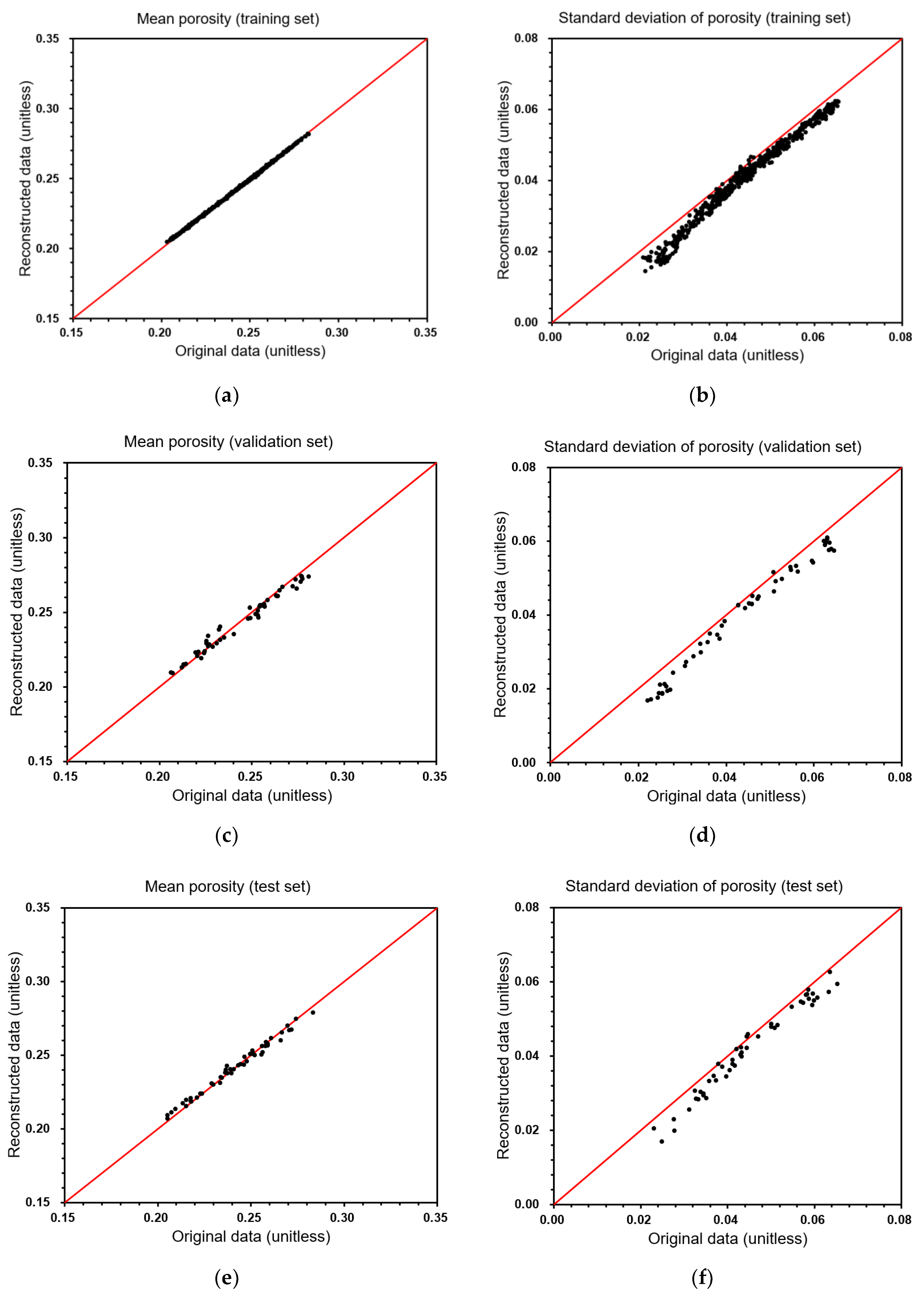
3.1. Reconstruction Performances of Rock Properties

The parameter size is examined with the comparison of typical fully-connected-layer-type (multi-layered-perceptron-type; MLP-type) autoencoder [37,38]. Table 2 shows the number of parameters used by a typical MLP-type autoencoder if we set the latent features used to be the same as those of our DCAE, i.e., the 1920 parameters that represent 4.3% of the input data (the original 44,460 three-dimensional spatial properties). Notwithstanding the fact that the details of designing the MLP-type autoencoder may differ according to the user’s purpose, the general architecture is configured; a symmetrical structure uses the node number set to 1/3 or more in the previous layer to prevent any excess information loss. The total number of parameters would be about 1.5 billion for the encoding and decoding processes and thereby it is not practical to train this kind of network from the viewpoint of computational efficiency.
Figure 4 explains the DCAE architecture in detail; Figure 4a demonstrates the encoding process that reduces (38 × 45 × 13 × 2) dimensions to a (5 × 6 × 2 × 32) dimensional latent code, and Figure 4b shows the decoding workflow to reconstruct spatial properties (permeability and porosity) that have the same dimensions as the original data (38 × 45 × 13 × 2). The latent features are significantly reduced in the input data, decreasing from 44,460 to 1920. Table 3 and Table 4 summarize the details of how our DCAE encodes and decodes the data. As shown in Table 3 and Table 4, the total number of parameters in the DCAE system is 2,303,466 (=1,864,992 + 438,474) which is only 0.155% of what a typical MLP-type autoencoder would need to use (refer to Table 2). Our fully-convolutional network consists of 27 convolutional layers and 18 batch normalizations. The ‘Adam’ optimizer is chosen after testing Adam, RMSprop, Adamax, and Adagrad optimizers. The activation function is ‘ReLU (rectified linear unit)’ and the He normal initializer is used [39,40]. The loss function is based on the mean squared error. The normalization of the input image is carried out based on the maximum pixel value and thus all inputs range between 0 and 1.
Figure 5 depicts DCAE training performances; here, the training loss and the validation loss values are compared. The local fluctuation observed in the trajectory of the validation loss is caused by the learning rates being updating. Both losses decrease steadily and converge to the minimum loss near the 350th epoch. The computation time is also fast achieving a rate of approximately 1.92 s/epoch (AMD Ryzen Threadripper 3960× 24-cores 3.79 GHz; 128 Gb RAM; NVIDIA Geforce RTX 2080Ti). The trends in Figure 5 confirm that DCAE-based feature extraction (dimensionality reduction) leads to stable convergence without overfitting while only incurring small computing costs and shows the efficiency of the DCAE architecture introduced in this study.
The DCAE reconstructs spatial properties reliably. Table 5 summarizes the reconstruction performance in terms of R-squared, RMSE, and MAPE. Figure 6 compares the mean and the standard deviation of the permeabilities from the original input and the reconstructed geo-models. For example, 22,230 (=38 × 45 × 13) permeability values are input; the DCAE reconstructed these for each geo-model, and thereby one mean and one standard deviation are evaluated for each geo-model. The DCAE training operation (for 500 geo-models) matches the mean permeability up to 0.999 for the R-squared value, 0.872 millidarcy for RMSE, and 0.18% for MAPE. The results for the mean permeability from the validation and test sets have slightly lower R-squared values than the training set, i.e., 0.997 for the validation set (50 geo-models) and 0.996 for the test set (50 geo-models), but these differences are small enough to confirm the reliability of the DCAE. The standard deviations of reconstructed permeabilities have slightly lower values than the original inputs, of which the reasons would be from the inevitable information loss during dimension compression. All performance metrics related to the standard deviations of the training, validation, and test sets show similar trends. The R-squared values of the standard deviations for permeabilities are 0.992 for the training set, 0.983 for validation, and 0.980 for the test set. Figure 7 depicts a comparison of the porosities between the original input and the reconstructed data. In a similar way to the results already shown in Figure 6, the porosity prediction is accurate and efficient. The R-squared values for mean porosity after reconstruction are 0.999 for the training set, 0.979 for the validation set, and 0.989 for the test set. The lowest R-squared value is 0.972 for the standard deviation of the porosities with the test set. Analyzing Figure 6 and Figure 7, as well as Table 5, it is clear that the DCAE is able to extract latent features and then reconstruct the spatial properties accurately.
In short, after evaluating the performance of the DCAE-based feature extraction, it can be concluded that the developed architecture can reduce the number of parameters required for reconstruction to just 2,303,466 for both encoding and decoding operations, which is only 0.155% of what a typical symmetric-autoencoder would require. The extracted features are reliable, which is shown by the small errors and the high R-squared values after reconstructing the original spatial values. Another notable conclusion is that the DCAE can integrate different spatial properties within a single architecture and also regenerate both spatial values accurately from a statistical viewpoint. The results confirm that the developed DCAE-based feature extraction can be applied efficiently for upscaling and downscaling spatial properties.

3.2. Surrogate Estimation for CO2 Geological Sequestration

An adaptive surrogate model is constructed to estimate CO2 sequestration as an alternative to time-consuming simulations. Figure 8 and Table 6 explain the detailed architecture of adaptive surrogate estimation using the features extracted from spatial data on permeability and porosity, the modeling parameters such as salinity and temperature, as well as the operating conditions such as the minimum well bottom hole pressure and the maximum CO2 injection rates. The input dimensions are (5 × 6 × 2 × 36) while there are three outputs after global average pooling. The model consists of a fully-convolutional neural network but while we do not implement the fully-connected layers, seven convolutional layers and seven batch normalizations are included. The number of parameters used for the adaptive surrogate estimation is 348,239.
Figure 9 shows the training and validation losses with epochs. The y-axis values are expressed as RMSE with units of million cubic meters to improve the understanding of training performances. The graph shows stable convergence and confirms that the model is efficient enough to converge to the final solutions without any remarkable fluctuations after 100 epochs. The computing time required is 0.09 s/epoch and no issues related to overfitting matters are experienced, and thus we can see that the surrogate model with the fully-convolutional network developed in this paper converges stably to the final optimality.
Figure 10 depicts the performances for estimating the output responses with the test set (50 geo-models), i.e., the structural trap amount (Figure 10a), the dissolved trap amount (Figure 10b), and the total CO2 volume injected into the aquifer (Figure 10c). Table 7 summarizes the results of the indicators used to evaluate the prediction performance. The highest R-squared value, 0.989, is observed for predicting the dissolved trap amount; a possible reason for this would be assigning salinity and temperature as the input units that influence CO2 dissolution. The heterogeneity of aquifer properties more strongly affects the structural trap amount and the total CO2 injected volume. However, the MAPEs are lower than that of the dissolved trap amount, which is 3.02% as shown in Table 7. Thus, we can conclude that both the spatial heterogeneity and operating conditions influence the predictability. A notable result is that the errors are less than 3.02% of the MAPE so that the adaptive surrogate estimation is accurate without the need for time-consuming physically-based simulations.
The large number of parameters involved in the deep-learning workflow cannot be free from ‘the curse of dimensionality’. The dimensionality reduction is essential to solve the following problems: convergence and computation efficiency. The high dimensions have sparse characteristics, the distance between training samples would be far, the extrapolation to forecast unknown values is unstable, and thus the overfitting and the poor convergence matters become more likely. In addition, the large number of operations, e.g., dot products between the kernel and the feature map, and the training parameters decrease the computational efficiency; the computing cost of adaptive surrogate estimation is 0.09 s/epoch. If analyzing the approximate computation time, the adaptive surrogate estimation requires 1005 s including the time for training over 500 epochs and estimating 50 test geo–models (=500 × (1.92 for DCAE + 0.09 for surrogate estimation); the prediction time is negligible. In contrast, the conventional flow simulations need 13,940 s to complete the 50 test geo–models(=278.8 × 50). Thus, the adaptive surrogate estimation can dramatically reduce the computational time required to approximately 7% of the time for the conventional flow simulation.
This study reduces the size of the feature map and convolutional operations required. In this way, an improvement of the computational efficiency is obtained. The methodology exploits the data integration within a single architecture unlike typical multimodal deep-learning approaches, and thus our method is able to successfully execute the reliable reconstruction of spatial properties as well as efficient dimensionality reduction.
An original part of the developed adaptive model in terms of methodology is that all inputs are integrally regarded as image channels from the initial stage of learning while typical multimodal models integrate the dataset within the flattened layers. Another key point is to use the fully-convolutional network and global average pooling instead of fully-connected layers, which is done to minimize the data loss without flattening the data to a one-dimensional array, and also to mitigate overfitting. Designing the proper hyper-parameters (such as the size of the feature map, the number of convolutional layers, kernel size, and the number of kernels, etc.) dominates the computational efforts, and thus the optimal designs that combine sub-sections of deep-learning will be challenging to reach the optimality of adaptive surrogate estimations. Notwithstanding that this paper shows successful estimation of three key results related to CO2 sequestration performance without using physically-based simulations, the spatiotemporal responses, e.g., saturation distribution and sequestration amount with time, need to be evaluated accurately in order to completely replace time-consuming subsurface flow simulations.

4. Conclusions

This paper presented an adaptive surrogate estimation based on a DCAE with fully-convolutional network that reduces the number of parameters needed without using typical fully-connected layers and flattening the spatial data. The DCAE-based feature extraction integrated different spatial data within one fully-convolution network and reliably reconstructed the original data. The fully-convolutional network significantly reduced the number of parameters to 0.155% of what a typical autoencoder would require. The reconstruction performance of spatial properties, i.e., permeability and porosity, proved to be reliable in achieving R-squared values higher than 0.972 for the mean and standard deviation of the test dataset.
Adaptive surrogate estimation was carried out using the spatial features extracted by our DCAE, the modeling parameters (salinity and temperature), and the operating conditions (well bottom hole pressure and CO2 injection rate). The surrogate model accurately estimated CO2 sequestration performances with R-squared values higher than 0.892 and mean absolute percentage error of less than 3.02% for the amounts of structural trap, dissolved trap, and total CO2 injection. The proposed DCAE-based surrogate estimation can be utilized for regression problems as well as for integration of scale-dependent spatial datasets.

Author Contributions

Conceptualization, S.J. and C.P.; methodology, S.J.; validation, S.J. and C.P.; formal analysis, S.A.; writing—original draft preparation, S.J. and S.A.; writing—review and editing, C.P. and D.-W.R.; supervision, D.-W.R.; funding acquisition, C.P. All authors have read and agreed to the published version of the manuscript.

Funding

This study was supported by the National Research Foundation of Korea (NRF) grant funded by the Korea government (MSIT) (No. 2020R1F1A1073395) and by the Ministry of Trade, Industry & Energy (MOTIE; Nos. 20172510102150; 20172510102160). In addition, it was supported by the basic research project of the Korean Institute of Geoscience and Mineral Resources (KIGAM) (GP2021–001;21–3117) funded by the Ministry of Science and ICT, Korea.

Institutional Review Board Statement

Not applicable.

Informed Consent Statement

Not applicable.

Data Availability Statement

Data sharing is not applicable.

Conflicts of Interest

The authors declare no conflict of interest.

References

  1. Schuetter, J.; Mishra, S.; Zhong, M.; LaFollette, R. A Data-Analytics Tutorial: Building Predictive Models for Oil Production in an Unconventional Shale Reservoir. SPE J. 2018, 23, 1075–1089. [Google Scholar] [CrossRef]
  2. Ertekin, T.; Sun, Q. Artificial Intelligence Applications in Reservoir Engineering: A Status Check. Energies 2019, 12, 2897. [Google Scholar] [CrossRef] [Green Version]
  3. Alakeely, A.; Horne, R.N. Simulating the Behavior of Reservoirs with Convolutional and Recurrent Neural Networks. SPE Reserv. Eval. Eng. 2020, 23, 992–1005. [Google Scholar] [CrossRef]
  4. Ki, S.; Jang, I.; Cha, B.; Seo, J.; Kwon, O. Restoration of Missing Pressures in a Gas Well Using Recurrent Neural Networks with Long Short-Term Memory Cells. Energies 2020, 13, 4696. [Google Scholar] [CrossRef]
  5. Seong, Y.; Park, C.; Choi, J.; Jang, I. Surrogate Model with a Deep Neural Network to Evaluate Gas–Liquid Flow in a Horizontal Pipe. Energies 2020, 13, 968. [Google Scholar] [CrossRef] [Green Version]
  6. Schuetter, J.; Mishra, K.S.; Ganesh, P.R.; Mooney, D. Building Statistical Proxy Models for CO2 Geologic Sequestration. Energy Procedia 2014, 63, 3702–3714. [Google Scholar] [CrossRef] [Green Version]
  7. Shahkarami, A.; Mohaghegh, S.; Gholami, V.; Haghighat, A.; Moreno, D. Modeling pressure and saturation distribution in a CO2 storage project using a Surrogate Reservoir Model (SRM). Greenh. Gases Sci. Technol. 2014, 4, 289–315. [Google Scholar] [CrossRef]
  8. Golzari, A.; Sefat, M.H.; Jamshidi, S. Development of an adaptive surrogate model for production optimization. J. Pet. Sci. Eng. 2015, 133, 677–688. [Google Scholar] [CrossRef]
  9. Tang, M.; Liu, Y.; Durlofsky, L.J. A deep-learning-based surrogate model for data assimilation in dynamic subsurface flow problems. J. Comput. Phys. 2020, 413, 109456. [Google Scholar] [CrossRef] [Green Version]
  10. Liu, Y.; Sun, W.; Durlofsky, L.J. A Deep-Learning-Based Geological Parameterization for History Matching Complex Models. Math. Geol. 2019, 51, 725–766. [Google Scholar] [CrossRef] [Green Version]
  11. Chu, M.-G.; Min, B.; Kwon, S.; Park, G.; Kim, S.; Huy, N.X. Determination of an infill well placement using a data-driven multi-modal convolutional neural network. J. Pet. Sci. Eng. 2020, 195, 106805. [Google Scholar] [CrossRef]
  12. Deng, X.; Tian, X.; Chen, S.; Harris, C.J. Deep learning based nonlinear principal component analysis for industrial process fault detection. In Proceedings of the 2017 International Joint Conference on Neural Networks (IJCNN), Anchorage, AK, USA, 14–19 May 2017; Institute of Electrical and Electronics Engineers (IEEE): Anchorage, AK, USA, 2017; pp. 1237–1243. [Google Scholar]
  13. Zhang, C.; Bengio, S.; Hardt, M.; Recht, B.; Vinyals, O. Understanding deep learning requires rethinking generalization. arXiv 2016, arXiv:1611.03530. Available online: https://arxiv.org/abs/1611.03530 (accessed on 10 January 2021).
  14. Canchumuni, S.W.A.; Emerick, A.A.; Pacheco, M.A.C. Towards a robust parameterization for conditioning facies models using deep variational autoencoders and ensemble smoother. Comput. Geosci. 2019, 128, 87–102. [Google Scholar] [CrossRef] [Green Version]
  15. Goodfellow, I.; Bengio, Y.; Courville, A. Deep Learning; MIT Press: Cambridge, MA, USA, 2016; ISBN 9780262035613. [Google Scholar]
  16. Schmidhuber, J. Deep learning in neural networks: An overview. Neural Netw. 2015, 61, 85–117. [Google Scholar] [CrossRef] [PubMed] [Green Version]
  17. O’Shea, K.; Nash, R. An introduction to convolutional neural networks. arXiv 2015, arXiv:1511.08458. Available online: https://arxiv.org/abs/1511.08458 (accessed on 10 January 2021).
  18. LeCun, Y.; Bengio, Y. Convolutional Networks for Images, Speech, and Time-Series. In The Handbook of Brain Theory and Neural Networks; Arbib, M.A., Ed.; MIT Press: Cambridge, MA, USA, 1995; Volume 3361. [Google Scholar]
  19. Yamashita, R.; Nishio, M.; Do, R.K.G.; Togashi, K. Convolutional neural networks: An overview and application in radiology. Insights Imaging 2018, 9, 611–629. [Google Scholar] [CrossRef] [Green Version]
  20. Razak, S.M.; Jafarpour, B. Convolutional neural networks (CNN) for feature-based model calibration under uncertain geologic scenarios. Comput. Geosci. 2020, 24, 1625–1649. [Google Scholar] [CrossRef]
  21. Ahn, S.; Park, C.; Kim, J.; Kang, J.M. Data-driven inverse modeling with a pre-trained neural network at heterogeneous channel reservoirs. J. Pet. Sci. Eng. 2018, 170, 785–796. [Google Scholar] [CrossRef]
  22. Kim, J.; Park, C.; Lee, K.; Ahn, S.; Jang, I. Deep neural network coupled with distance-based model selection for efficient history matching. J. Pet. Sci. Eng. 2020, 185, 106658. [Google Scholar] [CrossRef]
  23. Masci, J.; Meier, U.; Cireşan, D.; Schmidhuber, J. Stacked Convolutional Auto-Encoders for Hierarchical Feature Extraction. In Lecture Notes in Computer Science, Proceedings of the Lecture Notes in Computer Science, Espoo, Finland, 14–17 June 2011; Springer Science and Business Media LLC: New York, NY, USA, 2011; pp. 52–59. [Google Scholar]
  24. Cheung, C.M.; Goyal, P.; Prasanna, V.K.; Tehrani, A.S. OReONet: Deep convolutional network for oil reservoir optimization. In Proceedings of the 2017 IEEE International Conference on Big Data (Big Data), Boston, MA, USA, 11–14 December 2017; Institute of Electrical and Electronics Engineers (IEEE): Washington, DC, USA, 2017; pp. 1277–1282. [Google Scholar]
  25. Krizhevsky, A.; Sutskever, I.; Hinton, G.E. Imagenet classification with deep convolutional neural networks. In Proceedings of the Advances in Neural Information Processing Systems, Lake Tahoe, NV, USA, 3–6 December 2012; pp. 1097–1105. [Google Scholar]
  26. Maggipinto, M.; Masiero, C.; Beghi, A.; Susto, G.A. A Convolutional Autoencoder Approach for Feature Extraction in Virtual Metrology. Procedia Manuf. 2018, 17, 126–133. [Google Scholar] [CrossRef]
  27. Zhu, Y.; Zabaras, N. Bayesian deep convolutional encoder–decoder networks for surrogate modeling and uncertainty quantification. J. Comput. Phys. 2018, 366, 415–447. [Google Scholar] [CrossRef] [Green Version]
  28. Liu, M.; Grana, D. Petrophysical characterization of deep saline aquifers for CO2 storage using ensemble smoother and deep convolutional autoencoder. Adv. Water Resour. 2020, 142, 103634. [Google Scholar] [CrossRef]
  29. Yellig, W.F.; Metcalfe, R.S. Determination and Prediction of CO2 Minimum Miscibility Pressures (includes associated paper 8876). J. Pet. Technol. 1980, 32, 160–168. [Google Scholar] [CrossRef]
  30. Ioffe, S.; Szegedy, C. Batch normalization: Accelerating deep network training by reducing internal covariate shift. arXiv 2015, arXiv:1502.03167. [Google Scholar]
  31. Lin, M.; Chen, Q.; Yan, S. Network in network. arXiv 2014, arXiv:1312.4400v3. Available online: https://arxiv.org/pdf/1312.4400.pdf (accessed on 10 January 2021).
  32. Zhou, B.; Khosla, A.; Lapedriza, A.; Oliva, A.; Torralba, A. Learning Deep Features for Discriminative Localization. In Proceedings of the 2016 IEEE Conference on Computer Vision and Pattern Recognition, CVPR 2016, Las Vegas, NV, USA, 26 June–1 July 2016; IEEE: New York, NY, USA, 2016; pp. 2921–2929. [Google Scholar]
  33. Scherer, D.; Müller, A.; Behnke, S. Evaluation of Pooling Operations in Convolutional Architectures for Object Recognition. In Lecture Notes in Computer Science; Springer Science and Business Media LLC: New York, NY, USA, 2010; pp. 92–101. [Google Scholar]
  34. Glantz, S.A.; Slinker, B.K.; Neilands, T.B. Primer of Applied Regression & Analysis of Variance, 3rd ed.; McGraw-Hill: New York, NY, USA, 2016; ISBN 9780071824118. [Google Scholar]
  35. Hyndman, R.J.; Koehler, A.B. Another look at measures of forecast accuracy. Int. J. Forecast. 2006, 22, 679–688. [Google Scholar] [CrossRef] [Green Version]
  36. De Myttenaere, A.; Golden, B.; Le Grand, B.; Rossi, F. Mean Absolute Percentage Error for regression models. Neurocomputing 2016, 192, 38–48. [Google Scholar] [CrossRef] [Green Version]
  37. Erhan, D.; Bengio, Y.; Courville, A.; Manzagol, P.A.; Vincent, P.; Bengio, S. Why does unsupervised pre-training help deep learning? J. Mach. Learn. Res. 2010, 11, 625–660. Available online: https://dl.acm.org/doi/10.5555/1756006 (accessed on 10 January 2021).
  38. Kramer, M.A. Nonlinear principal component analysis using autoassociative neural networks. AIChE J. 1991, 37, 233–243. [Google Scholar] [CrossRef]
  39. He, K.; Zhang, X.; Ren, S.; Sun, J. Delving deep into rectifiers: Surpassing human-level performance on imagenet classification. In Proceedings of the IEEE International Conference on Computer Vision, Santiago, Chile, 7–13 December 2015; IEEE: Piscataway, NJ, USA, 2015; pp. 1026–1034. [Google Scholar]
  40. Abadi, M.; Barham, P.; Chen, J.; Davis, A.; Dean, J.; Devin, M.; Ghemawat, S.; Irving, G.; Isard, M.; Kudlur, M. Tensorflow: A system for large-scale machine learning. In Proceedings of the 12th USENIX Symposium on Operating Systems Design and Implementation (OSDI’16), Savannah, GA, USA, 2–4 November 2016; Available online: https://www.usenix.org/system/files/conference/osdi16/osdi16-abadi.pdf (accessed on 10 January 2021).
Figure 1. Examples of 3D heterogeneous saline aquifers: (a) permeability distribution; (b) porosity distribution; (c) CO2 saturation at y = 25 plane after 50 years (well bottom hole pressure = 15 MPa and CO2 injection rate = 0.6 ×10⁶ m3/day).
Energies 14 00413 g001
Figure 2. The DCAE architecture proposed in this study: (a) the encoder extracts latent features from spatial properties (permeability and porosity); (b) the decoder conducts the inverse mapping of the latent features to the original dimensions and evaluates the reconstruction performance. Input data are also traversed by dilated kernels at the first convolution stage (gray); The feature map size is adjusted by strided convolution (red), transposed convolution (purple), and zero-padding (green); The cross-channel pooling with unit-sized kernel is introduced to reduce the parameter number.
Energies 14 00413 g002
Figure 3. Adaptive surrogate model developed in this study. It uses the latent features encoded by DCAE, the modeling parameters (temperature and salinity), and the operation conditions (the minimum WBHP—well bottom hole pressure—and the maximum CO2 injection rate).
Energies 14 00413 g003
Figure 4. The DCAE design and the dimensions of each stage: (a) the encoder to result in latent features with dimensionality reduction of network input; (b) the decoder to reconstruct the spatial properties.
Energies 14 00413 g004
Figure 5. Training performance of DCAE-based feature extraction (dimensionality reduction). The loss function is the mean squared error.
Energies 14 00413 g005
Figure 6. Geo-model reconstruction performance of DCAE for permeability: (a) mean values of permeabilities from 500 geo-models (training set); (b) standard deviations of permeabilities from 500 geo-models (training set); (c) mean values of permeabilities from 50 geo-models (validation set); (d) standard deviations of permeabilities from 50 geo-models (validation set); (e) mean values of permeabilities from 50 geo-models (test set); (f) standard deviations of permeabilities from 50 geo-models (test set). Each black point is calculated for each geo-model using 22,230 grid values.
Energies 14 00413 g006
Figure 7. Geo-model reconstruction performance of DCAE for porosity: (a) mean values of porosities from 500 geo-models (training set); (b) standard deviations of porosities from 500 geo-models (training set); (c) mean values of porosities from 50 geo-models (validation set); (d) standard deviations of porosities from 50 geo-models (validation set); (e) mean values of porosities from 50 geo-models (test set); (f) standard deviations of porosities from 50 geo-models (test set). Each black point is calculated for each geo-model using 22,230 grid values.
Energies 14 00413 g007
Figure 8. Architecture of the adaptive surrogate model using the feature extracted by our DCAE, the modeling parameters, and the operating conditions. WBHP stands for well bottom hole pressure.
Energies 14 00413 g008
Figure 9. Training performances of the adaptive surrogate model. The loss function is originally chosen to be the mean squared error. The values on the y-axis have been transformed to root mean squared errors where the units are million cubic meters (MMm3).
Energies 14 00413 g009
Figure 10. Performances of the adaptive surrogate model to estimate the outputs in the test set (50 geo-models): (a) structural trap volume; (b) dissolved trap volume; (c) total CO2 volume injected into the saline aquifers. MMm3: million cubic meters (×106 m3).
Energies 14 00413 g010
Table 1. Statistical properties to generate heterogeneous geo-models.
PropertyValue Range
1 Permeability (millidarcy)100~1000 (sandstone), 1~10 (shale)
Porosity (unitless)0.2~0.3 (sandstone), 0.1~0.15 (shale)
Shale volume ratio (%)1~20
Temperature (Celsius)40~50
2 Salinity (ppm)100,000~250,000
1 millidarcy: 1 millidarcy = 9.869 × 10⁻¹⁰ m2; 2 ppm: Part Per Million.
Table 2. Comparison case to train the symmetric MLP-type autoencoder.
DescriptionOutput ShapeThe Number of Parameters
EncoderNetwork input(44,460)-
Hidden layer 1(14,820)658,912,020
Hidden layer 2(4940)73,215,740
Hidden layer 3(1920)9,486,720
Encoder total-741,614,480
DecoderHidden layer 4(4940)9,489,740
Hidden layer 5(14,820)73,225,620
Network output(44,460)658,941,660
Decoder total-741,657,020
Network total-1,483,271,500
Table 3. Detailed design of the DCAE encoder.
Layer DescriptionKernelsOutput ShapeThe Number of ParametersRemark
Network input (38, 45, 13, 2)--
1 Conv 116, (3 × 3 × 3)(38, 45, 13, 16)880-
2 BN 1-(38, 45, 13, 16)64
Convn 216, (3 × 3 × 3)(38, 45, 13, 16)880Dilated kernel
BN 2-(38, 45, 13, 16)64
Concatenate-(38, 45, 13, 32)--
Conv 332, (3 × 3 × 3)(38, 45, 13, 32)27,680-
BN 3-(38, 45, 13, 32)128
Conv 464, (2 × 2 × 2)(19, 23, 7, 64)16,448Strided convolution
BN 4-(19, 23, 7, 64)256
Conv 564, (3 × 3 × 3)(19, 23, 7, 64)110,656-
BN 5-(19, 23, 7, 64)256
Conv 664, (3 × 3 × 3)(19, 23, 7, 64)110,656-
BN 6-(19, 23, 7, 64)256
Conv 7128, (2 × 2 × 2)(10, 12, 4, 128)65,664Strided convolution
BN 7-(10, 12, 4, 128)512
Conv 864, (1 × 1 × 1)(10, 12, 4, 64)8256Cross-channel pooling
BN 8-(10, 12, 4, 64)256
Conv 9128, (3 × 3 × 3)(10, 12, 4, 128)221,312-
BN 9-(10, 12, 4, 128)512
Conv 1064, (1 × 1 × 1)(10, 12, 4, 64)8256Cross-channel pooling
BN 10-(10, 12, 4, 64)256
Conv 11128, (3 × 3 × 3)(10, 12, 4, 128)221,312-
BN 11-(10, 12, 4, 128)512
Conv 1264, (1 × 1 × 1)(10, 12, 4, 64)8256Cross-channel pooling
BN 12-(10, 12, 4, 64)256
Conv 13256, (2 × 2 × 2)(5, 6, 2, 256)131,328Strided convolution
BN 13-(5, 6, 2, 256)1024
Conv 1464, (1 × 1 × 1)(5, 6, 2, 64)16,448Cross-channel pooling
BN 14-(10, 12, 4, 64)256
Conv 15256, (3 × 3 × 3)(5, 6, 2, 256)442,624-
BN 15-(5, 6, 2, 256)1024
Conv 1664, (1 × 1 × 1)(5, 6, 2, 64)16,448Cross-channel pooling
BN 16-(10, 12, 4, 64)256
Conv 17256, (3 × 3 × 3)(5, 6, 2, 256)442,624-
BN 17-(5, 6, 2, 256)1024
Conv 1832, (1 × 1 × 1)(5, 6, 2, 32)16,448Cross-channel pooling
BN 18-(5, 6, 2, 32)256
Encoder total1,864,992
1 Conv: convolutional layer; 2 BN: Batch Normalization.
Table 4. Detailed design of the DCAE decoder.
Layer DescriptionKernelsOutput ShapeThe Number of ParametersRemark
Decoder input (5, 6, 2, 32)--
1 Conv 19 128, (3 × 3 × 3)(5, 6, 2, 128)110,720-
2 BN 19-(5, 6, 2, 128)512
Conv 20 64, (1 × 1 × 1)(5, 6, 2, 64)8256Cross-channel pooling
BN 20-(5, 6, 2, 64)256
Conv 21 128, (3 × 3 × 3)(5, 6, 2, 128)221,312-
BN 21-(5, 6, 2, 128)512
Conv 22 64, (2 × 2 × 2)(10, 12, 4, 64)65,600Transposed convolution
BN 22-(10, 12, 4, 64)256
Conv 23 32, (2 × 2 × 2)(20, 24, 8, 32)16,416Transposed convolution
BN 23-(20, 24, 8, 32)128
Conv 2432, (2 × 2 × 2)(19, 23, 7, 32)8224Convolution without zero-padding
BN 24-(19, 23, 7, 32)128
Conv 25 16, (2 × 2 × 2)(38, 46, 14, 16)4112Transposed convolution
BN 25-(38, 46, 14, 16)64
Conv 2616, (1×2×2)(38, 45, 13, 16)1040Convolution without zero-padding
BN 26-(38, 45, 13, 16)64
Conv 272, (3 × 3 × 3)(38, 45, 13, 2)866-
BN 27-(38, 45, 13, 2)8
Decoder Total438,474
1 Conv: convolutional layer; 2 BN: Batch Normalization.
Table 5. Summary of results from the evaluation of the reconstruction performances of our DCAE network.
Data SetPermeabilityPorosity
MeanStandard DeviationMeanStandard Deviation
R2
(R-squared)
Training set0.9990.9920.9990.985
Validation set0.9970.9830.9790.985
Test set0.9960.9800.9890.972
1RMSETraining set0.87211.560.00070.0037
Validation set9.4814.360.0050.0042
Test set9.9314.610.0030.0038
2MAPE (%)Training set0.184.850.258.64
Validation set1.905.921.2110.40
Test set1.795.850.858.25
1 RMSE: Root Mean Squared Error; 2 MAPE: Mean Absolute Percentage Error. For RMSE, the units of mean and standard deviation for permeability are millidarcy while porosity is unitless.
Table 6. Detailed design of the adaptive surrogate model using a deep convolutional neural network.
Layer DescriptionKernelsOutput ShapeThe Number of ParametersRemark
Network input (5, 6, 2, 36)--
1 Conv 1 64, (3 × 3 × 2)(5, 6, 2, 64)41,536
2 BN 1-(5, 6, 2, 64)256
Conv 2 64, (3 × 3 × 2)(5, 6, 2, 64)73,792
BN 2-(5, 6, 2, 64)256
Conv 3 128, (2 × 2 × 2)(3, 3, 1, 128)65,664Strided convolution
BN 3-(3, 3, 1, 128)512
Conv 4 128, (2 × 2 × 1)(3, 3, 1, 128)65,664
BN 4-(3, 3, 1, 128)512
Conv 5 128, (2 × 2 × 1)(3, 3, 1, 128)65,664
BN 5-(3, 3, 1, 128)512
Conv 6 64, (2 × 2 × 1)(3, 3, 1, 64)32,832
BN 6-(3, 3, 1, 64)256
Conv 73, (2 × 2 × 1)(3, 3, 1, 3)771
BN 7-(3, 3, 1, 3)12
Global average pooling (3)-
Network Total 348,239
1 Conv: convolutional layer; 2 BN: Batch Normalization.
Table 7. Results of adaptive surrogate estimation for CO2 sequestration performances (test set).
Structural TrapDissolved TrapTotal CO2 Volume Injected
R2 (R-squared)0.8920.9890.951
1RMSE (MMm3)56.5311.14115.38
2MAPE (%)2.883.022.80
1 RMSE: Root Mean Squared Error; MMm3: million cubic meters (×106 m3); 2 MAPE: Mean Absolute Percentage Error.
Publisher’s Note: MDPI stays neutral with regard to jurisdictional claims in published maps and institutional affiliations.

