A Multivariate High-Order Markov Model for the Income Estimation of a Wind Farm

Abstract

The energy produced by a wind farm in a given location and its associated income depends both on the wind characteristics in that location—i.e., speed and direction—and the dynamics of the electricity spot price. Because of the evidence of cross-correlations between wind speed, direction and price series and their lagged series, we aim to assess the income of a hypothetical wind farm located in central Italy when all interactions are considered. To model these cross and auto-correlations efficiently, we apply a high-order multivariate Markov model which includes dependencies from each time series and from a certain level of past values. Besides this, we used the Raftery Mixture Transition Distribution model (MTD) to reduce the number of parameters to get a more parsimonious model. Using data from the MERRA-2 project and from the electricity market in Italy, we estimate the model parameters and validate them through a Monte Carlo simulation. The results show that the simulated income faithfully reproduces the empirical income and that the multivariate model also closely reproduces the cross-correlations between the variables. Therefore, the model can be used to predict the income generated by a wind farm.

1. Introduction

The production of energy from renewable sources has been undergoing a significant increase in recent years. More specifically, the energy produced from wind power has achieved a 10% increase in the worldwide capacity and 19% increase of installations from 2018 to 2019 due to its availability throughout the day and relatively low cost of transformation [1]. Despite that, when dealing with the income generated from selling the energy produced from a wind power plant, one has to consider two main sources of uncertainty: wind speed and energy prices. In fact, both variables have a random nature that should be considered when building a model [2].

The energy produced by a wind turbine, and more generally by a wind power plant, is subject to considerable fluctuations over time related to the characteristics of wind and the location of the plant [3]. The random trend of wind concerns both its speed and its direction [4,5]. In fact, it is shown that these two variables are correlated. In addition, wind speed and direction are also log range autocorrelated.

The modelling of energy produced by a wind turbine was examined by D’Amico et al. [6] using an indexed semi-Markov model to reproduce the statistical behaviour of wind speed. Then, in [7], the model was extended to a multivariate setting to estimate the energy produced by a wind farm. The authors used a copula function to represent the spatial non-linear dependencies of the systems’ energy production. In [4], Votsi and Brouste applied semi-Markov models to wind power production. The authors investigated the mean time to failure in the context of reliability. Next, an additional application of semi-Markov processes was proposed by Danisman and Kocer [8] about handling missing data. Song and Paek [9] studied the dynamic simulations of a wind turbine to predict its annual energy production using a computational fluid dynamics code for wind farm. Lopez et al. [10] predicted wind speed in the short-term using three non-parametric statistical regression techniques. Moreover, other authors used particular transformations of the data, such as Box–Cox and the normal inverse Gaussian transformation, to obtain data closer to a Gaussian distribution [11,12,13]. Indeed, it is well known in the literature that wind speed distribution is typically well reproduced by Weibull distributions [14]. Besides this, another feature of the distribution of wind speed is the presence of fat tails [15,16].

Regarding the financial aspects, the income generated from the selling of produced energy depends on the spot electricity price. The income is usually determined as the sum of the discounted values of the product between the energy generated and the price in that particular area. The income will, therefore, be subject not only to the random wind trend, and therefore to the energy produced, but also to the uncertainty of the spot price of electricity [17]. The income of a wind farm has been investigated by [18]. The authors applied an Ornstein–Uhlenbeck process to model wind speed and energy production and an inverse Gaussian process to represent the logarithm of electricity spot prices. Recently, it has been shown that spot price and wind speed are correlated [2]. The authors modelled the stochastic variables for wind speed and the spot price of electricity using econometric processes, while the dependency structure was managed through copula functions. However, they did not consider the direction in their model.

It is evident that to effectively model the income produced by a wind power plant, one has to build a multivariate model that takes into account all the characteristics described above. To this end, a multivariate high-order Markov model can be applied. In general, high-order Markov models have been successfully implemented by many authors. For example, Raftery [19] proposed the Mixture Transition Distribution model (MTD) to analyse the time series of wind speed, while the same model applied to the wind direction was introduced in [20] and further analysed in [21]. On the contrary, the multivariate Markov model, introduced by [22] for categorical data, has been recently implemented in the analysis of financial time series. D’Amico and De Blasis [23] proposed a multivariate stochastic dividend discount model based on the MTD model, while De Blasis [24] applied the same model to the analysis of price discovery in financial markets. Besides, the MTD model by [19] helps in reducing the number of parameters to obtain a more parsimonious model for a comprehensive review of the MTD model, readers can refer to [25]).

In this work, we propose to use a multivariate high-order Markov chain to model the three variate processes of wind speed, wind direction and electricity price. In this way, we are able to consider both the dependence between the three variables and the long range autocorrelation for each of them. To overcome the problem related to the estimation of a huge number of parameters, we used a Mixture Transition Distribution. The ability of the model to reproduce real data is verified by a numerical application through Monte Carlo simulations. We consider wind and electricity price data for a hypothetical turbine located in central Italy. In our analysis, we consider data on a hourly basis. We take as a reference price the zonal market pertaining to the area in which the plant is located. The model is used to estimate the income that can be obtained from a wind farm. Finally, we compare the real data with the simulated data to determine whether our model produces reliable results.

The next sections are structured as follows. Section 2 describes the characteristics of the database used and the general model, while the results are presented in Section 3. Discussions and conclusions are given in Section 4 and Section 5, respectively.

2. Materials and Methods

This section describes the characteristics of the data used for the analysis. The data include information about wind speed and direction as well as prices of electricity for a hypothetical wind farm located in Central Italy with coordinates of 42 N and 13.75 E. The data frequency is hourly for 5 years, from 1 July 2015 to 30 June 2020, amounting to a total of 43,848 observations.

2.1. Wind Speed and Direction

Wind speed and direction data were downloaded from the MERRA-2 project [26]. The MERRA-2 model produces wind data at 2, 10 and 50 m from the ground. Because of the characteristic height of the wind turbines, we used the data at 50 m.

Table 1. Wind speed statistics for the location 42° N and 13.75° E (Central Italy). Speed in m/s. Hourly data from 1 July 2015 to 30 June 2020.

Year	Mean	Std	Skew	Kurt	Min	Max
1	3.31	2.34	1.63	3.39	0.01	15.82
2	3.47	2.44	1.66	3.03	0.05	16.34
3	3.64	2.41	1.41	2.45	0.03	16.30
4	3.46	2.27	1.48	2.91	0.06	16.17
5	3.54	2.53	1.74	3.73	0.05	17.53
Full	3.48	2.40	1.60	3.15	0.01	17.53

shows the summary statistics of the wind speed for each year, which appear to be quite constant for all the figures. In fact, the average speed moved from 3.31 m/s in year 1 to 3.54 m/s in year 5, with values that were compatible with the 5 year average. Moreover, the standard deviation during the five years was aligned around the value of 2.40 m/s. Furthermore, Figure 1 depicts the histogram along with the full time series of the wind speed, indicating that the wind speed followed a Weibull distribution, as confirmed by the probability plot in Figure 2.

We also include the wind direction to obtain a better model of the wind speed and thus electricity prices in the multivariate process. A graphical overview of the direction, grouped by different speeds, is provided in Figure 3. For the coordinates that we consider in this analysis, the wind blows mostly from the northeast and, with less frequency, from the south. Moreover, the polar plot shows a clear relation between wind speed and direction, demonstrated by the high peaks of wind speed around the northeast and the south–southwest direction.

2.2. Wind Energy Production

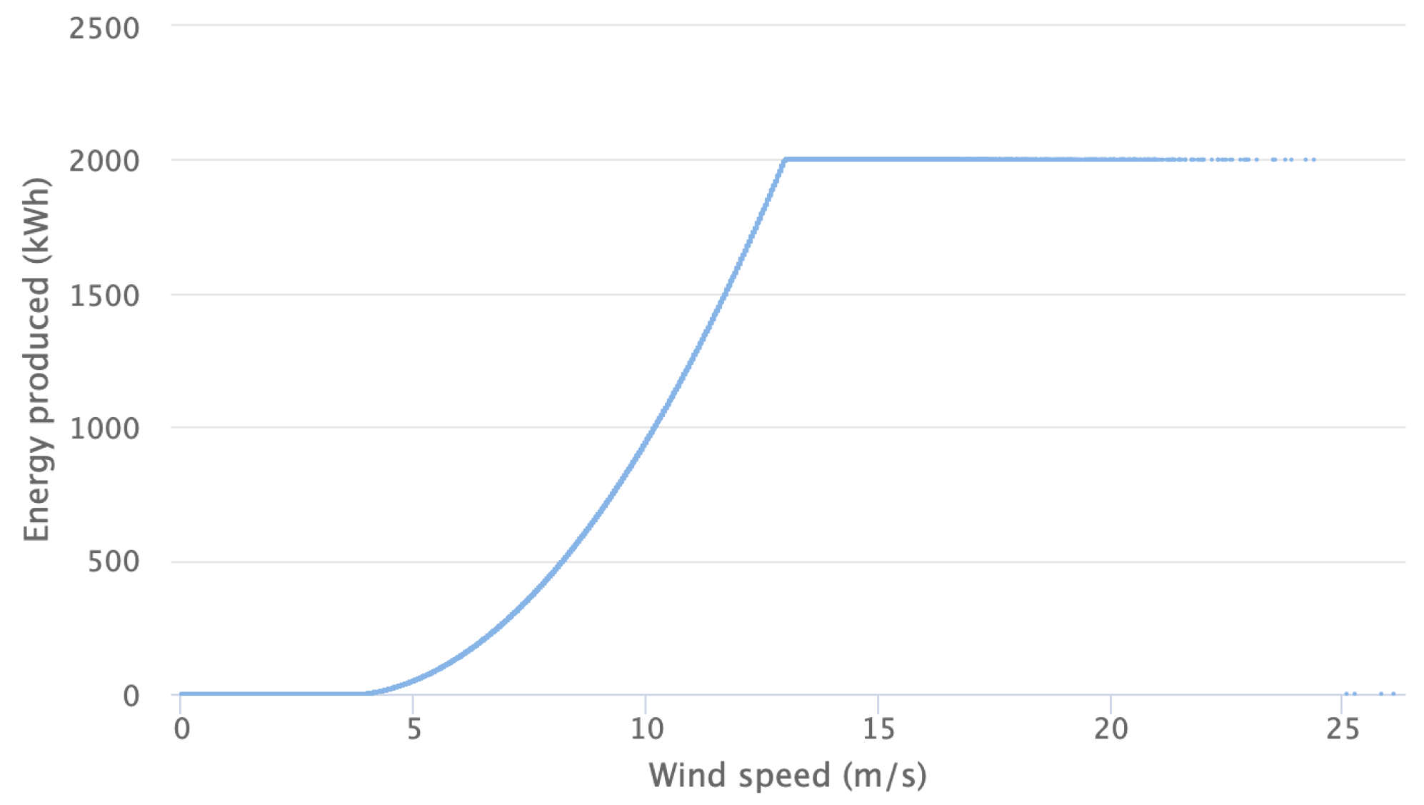
To obtain an estimation of the wind turbine income, we needed to convert the wind speed to energy production. Wind turbines transform the kinetic energy of wind into electrical power through the rotational movement of the blades. The amount of energy produced depends on the wind intensity, as well as on the characteristics of the blades. For this purpose, the turbine is characterised by its power curve, which is generally given by the turbine producer. In our application, we considered a generic wind turbine with the following characteristics:

• Hub height of the turbine: 95 m;
• Rated power of the turbine: 2 MW;
• Cut-in wind speed: 4 m/s;
• Rated wind speed: 13 m/s;
• Cut-out wind speed: 25 m/s.

In general, the power curve is linked to two critical values for wind speed. Below the first threshold—i.e., the cut-in value—the turbine does not produce energy at all, meaning that the kinetic energy of the wind is too weak to move the blades. In addition, above the second threshold—i.e., the cut-off value—the turbine is blocked to avoid structural damage. Between these two limits, there is a cubic relation, known as the Betz law, which links the wind speed with the energy produced. This typical behaviour of the wind turbine production is clearly evident in Figure 4, which shows the power curve given by the producer of the turbine considered in our application. Besides, taking into account that the wind data were generated for a height of 50 m and the wind turbine height was at 95 m, we used an exponential scaling factor, as in [15], using the following dependence from the altitude:

$$v_h=v_{rif}{\left(\frac{h}{h_{rif}}\right)}^{\alpha }\alpha =\frac{1}{ln\frac{h}{z_0}}$$

(1)

where $v_h$ is the wind speed at the height of the wind turbine, $v_{rif}$ is the value of the wind speed at 50 m—in our application $h=50$ m and $h_{rif}=95$ m—and $z_0$ is a factor that takes into account the morphology of the area near the wind turbine. This parameter depends on the region in which the turbine is located. Its value ranges from 0.01 and 0.001 depending on buildings or trees in the area; for offshore application, it is equal to 0.0001. For our analysis, we considered a mean value for an onshore application; thus, we choe $z_0$ = 0.005.

2.3. Electricity Price

Electricity data were downloaded from the Italian Day-Ahead-Market (MGP), which is split into geographical areas. For our analysis, we selected the central southern zonal price, which reflects the location of our wind turbine. The Italian electricity market is an auction market that takes place one day in advance at 12 p.m. Prices for each zone and each hour of the next day are set during the auction, including the definition of the national unique price (PUN) as the weighted average of the prices with zonal volumes as weights. The hourly price series are available at the Mercato Elettrico website [27].

Table 2. Summary statistics of the electricity price for central–southern Italy. Prices in €/MWh. Hourly data from 1 July 2015 to 30 June 2020.

Year	Mean	Std	Skew	Kurtosis	Min	Max
1	45.57	15.57	1.36	3.73	10.0	146.33
2	47.20	12.88	1.61	5.22	10.0	150.00
3	54.22	15.73	1.65	6.22	0.0	170.00
4	61.34	13.38	0.06	2.37	0.0	141.25
5	41.42	15.18	0.04	-0.23	0.0	99.61
Full	49.95	16.20	0.70	2.26	0.0	170.00

shows the electricity price summary statistics divided by year for the central–southern Italian prices. Prices appear to be highly volatile with an annual standard deviation ranging from 12.88 to 16.20 €/MWh and with a 5 year average of 49.95 €/MWh. In the analysed periods, the peak reached the value of 170 €/MWh. In addition, Figure 5 depicts the histogram of the prices along with the full time-series for the five years. The price series fails the Jarque–Bera test of normality, as also reported in the probability plot in Figure 6, where the tails are clearly outside the normality assumption as shown from the kurtosis values in the summary statistics table.

2.4. Correlation

The analysis of the autocorrelation and partial autocorrelation function for the three time series, wind speed, direction and price, as reported in Figure 7, shows that all the series present a certain degree of dependency from the past values. Moreover,

Table 3. Cross-correlations between series and time lags.

	Price	Speed	Direction (Dir)
Price	1.000	–0.143	0.015
Speed	–0.143	1.000	–0.085
Dir	0.015	–0.085	1.000
Price L1	0.933	–0.139	0.029
Speed L1	–0.138	0.983	–0.089
Dir L1	–0.006	–0.073	0.860
Price L2	0.832	–0.129	0.033
Speed L2	–0.127	0.943	–0.088
Dir L2	–0.026	–0.058	0.745

reports the correlation coefficients for the three series, up to the second time lag. The contemporaneous correlation between price and speed shows a negative coefficient of –0.143. Even though there is a correlation that is almost close to zero between price and direction, the effect of the direction is propagated to the price through the wind speed. This pattern is also persistent when considering the time lags. Therefore, it seems appropriate to adopt a multivariate model which includes a certain level of dependency from the past values. Specifically, considering the partial autocorrelation function, a model with two lags should suffice for our purpose.

2.5. Model

The analysis of wind speed and price data clearly shows that there are cross-correlations between the series and the lagged series, suggesting the use of a multivariate model that considers some history of the process. A good candidate could be the multivariate Markov model with the inclusion of the dependencies from a certain level of past values. However, a Markov chain model would require the estimation of the probabilities of all possible combination of the transitions from one state to another for each series and each lag. In such a model, the number of parameters to estimate is liable to drastically increase with the number of states, series and time lags.

To overcome the estimation issue in the high-order Markov chains, in [19], the authors proposed the Mixture Transition Distribution model (MTD) to reduce the number of parameters in the estimation. Moreover, in [22], the authors applied the same approach to the multivariate Markov chains. In this paper, we propose a combination of the two approaches to deal simultaneously with high-order Markov chains and multivariate Markov chains.

In general, for a given Markov process $\mathbf{X}=(X_0,X_1,\cdots ,X_t)$, taking values in the set $\mathcal{M}=\{1,2,\cdots ,m\}$, the Markov property for its high-order chain can be written as

$$\mathbf{P}(X_t=i_0|X_0=i_t,\cdots ,X_{t-1}=i_1)=\mathbf{P}(X_t=i_0|X_{t-l}=i_l,\cdots ,X_{t-1}=i_1),$$

(2)

where $i_t,\cdots ,i_1,i_0\in \mathcal{M}$ and l is the order of the chain; i.e., the number of time lags.

Equation (2) states that the probability of being in state $i_0$ at time t does not depend on the full historical path of the process but only on the states occupied by it during the last l transitions. Therefore, the present case depends on the last l observations only.

According to [19], the high-order Markov property can be rewritten, on the basis of the MTD model, by the following relation:

$$\mathbf{P}(X_t=i_0|X_{t-l}=i_l,\cdots ,X_{t-1}=i_1)=\sum _{g=1}^l{\lambda }_g\mathbf{P}(X_t=i_0|X_{t-g}=i_g).$$

(3)

This property declares that the probability of being in state $i_0$ at time t still depends on the l states occupied by the process at previous time lags, but this dependency is represented by a linear combination of the probabilities of transitioning from state $i_g$ at time $t-g$ to state $i_0$ at time t. Therefore, based on the MTD model, we need to estimate l transition probability matrices whose entries represent the probability of transitioning from state $i_g$ to state $i_0$. Let $q_{i_g,i_0}$ be the transition probability from state $i_g$ at time $t-g$ to state $i_0$ at time t; the property in (3) can be written as

$$\sum _{g=1}^l{\lambda }_g\mathbf{P}(X_t=i_0|X_{t-g}=i_g)=\sum _{g=1}^l{\lambda }_g{q}_{i_g,i_0}.$$

(4)

However, if we consider a homogeneous Markov chain with states taking values in the set $M=\{1,\cdots ,m\}$, the process can be fully described by a probability vector ${\mathcal{X}}_t=(P(X_t=1),\cdots ,P(X_t=m))$ and a time-independent transition probability matrix $\mathbf{Q}$ whose entries $q_{i,i_0}$ are the probabilities of transitioning from state i, independent of the lag, to state $i_0$. Thus, the probability distribution at time t can be expressed in terms of the one-step transition as

$${\mathcal{X}}_t={\mathcal{X}}_{t-1}\mathbf{Q},$$

(5)

or, given an initial probability distribution vector, ${\mathcal{X}}_0$, as

$${\mathcal{X}}_t={\mathcal{X}}_0{\mathbf{Q}}^t.$$

(6)

With the homogeneity condition, the relation in (4) can be updated as

$$\sum _{g=1}^l{\lambda }_g\mathbf{P}(X_t=i_0|X_{t-g}=i_g)=\sum _{g=1}^l{\lambda }_g{q}_{i,i_0},$$

(7)

with $q_{i,i_0}$ being an element of the matrix $\mathbf{Q}$ that represents the probability of transitioning from state i to state $i_0$.

To ensure that we deal with probabilities in Equation (7), we need to ensure that

$$0\le \sum _{g=1}^l{\lambda }_g{q}_{i,i_0}\le 1,$$

implying the following conditions:

$$\sum _{g=1}^l{\lambda }_g=1,{\lambda }_g\ge 0.$$

(8)

Considering the convex linear combination presented in Equation (7), we have to estimate fewer parameters compared to the full high-order Markov chain. Specifically, we have $m(m-1))$ parameters for the transition probability matrix with m states plus $l-1$ values for the ${\lambda }_g$ coefficients, compared to a total of $m^l(m-1)$ parameters for a full high-order Markov chain.

For a comprehensive review of the MTD model and its applications, we refer the reader to [25].

The same MTD model approach can be applied to the multivariate Markov process. We now consider $\Gamma =\{1,\cdots ,\gamma \}$ series without including the time lags. In this case, the property in (3) becomes

$$\begin{array}{cc}\hfill & \mathbf{P}\left[X_t^{\alpha }=i_0^{\alpha }|(X_0^1=i_t^1,\cdots ,X_{t-1}^1=i_1^1),\cdots ,(X_0^1=i_t^{\gamma },\cdots ,X_{t-1}^{\gamma }=i_1^{\gamma })\right]\hfill \\ \hfill & =\sum _{\beta =1}^{\gamma }{\lambda }^{\beta \alpha }\mathbf{P}\left[X_t^{\alpha }=i_0^{\alpha }|(X_{t-1}^{\beta }=i_1^{\beta })\right],\hfill \end{array}$$

(9)

with $\alpha ,\beta \in \Gamma$.

This property states that the probability of being in a determined state at time t depends on the states occupied by all series at time $t-1$, according to a linear combination of the transition probability matrices ${\mathbf{Q}}^{\beta \alpha }$. Each element of these matrices represents the probability of transitioning from state i in series $\beta$ at time $t-1$ to state $i_0$ in series $\alpha$ at time t, as indicated in the following matrix:

$${\mathbf{Q}}^{\left(\beta \alpha \right)}=\begin{array}{cc}& X_t^{\alpha }\\ X_{t-1}^{\beta }& \begin{array}{cccc}1 \hspace{1em}& 2\hspace{1em}& \cdots & m\end{array}\\ \begin{array}{c}1\\ 2\\ ⋮\\ m\end{array}& \left[\begin{array}{cccc}{q}_{11}^{\beta \alpha }& q_{12}^{\beta \alpha }& \cdots & q_{1m}^{\beta \alpha }\\ q_{21}^{\beta \alpha }& q_{22}^{\beta \alpha }& \cdots & q_{2m}^{\beta \alpha }\\ ⋮& ⋮& \ddots & ⋮\\ q_{m1}^{\beta \alpha }& q_{m2}^{\beta \alpha }& \cdots & q_{mm}^{\beta \alpha }\end{array}\right]\end{array}.$$

(10)

Therefore, we need to estimate ${\gamma }^2$ matrices with $m(m-1)$ parameters, plus ${\gamma }^2$ values for the ${\lambda }^{\beta \alpha }$ coefficients. The total number of parameters to estimate for a multivariate Markov chain is ${\gamma }^2(m(m-1)+1)$.

As for the high-order Markov model, the multivariate Markov model is subject to the same conditions in (8):

$$\sum _{\beta =1}^{\gamma }{\lambda }^{\beta \alpha }=1,{\lambda }^{\beta \alpha }\ge 0.$$

(11)

For our purpose, we combine the previously described models and propose a high-order multivariate Markov model. The properties in Equations (7) and (9) can be jointly written as

$$\begin{array}{cc}\hfill & \mathbf{P}\left[X_t^{\alpha }=i_0^{\alpha }|(X_0^1=i_t^1,\cdots ,X_{t-1}^1=i_1^1),\cdots ,(X_0^1=i_t^{\gamma },\cdots ,X_{t-1}^{\gamma }=i_1^{\gamma })\right]\hfill \\ \hfill & =\sum _{\beta =1}^{\gamma }{\lambda }^{\beta \alpha }\mathbf{P}\left[X_t^{\alpha }=i_0^{\alpha }|(X_{t-l}^{\beta }=i_l^{\beta }),\cdots ,(X_{t-1}^{\beta }=i_1^{\beta })\right]\hfill \\ \hfill & =\sum _{\beta =1}^{\gamma }\sum _{g=1}^l{\lambda }_g^{\beta \alpha }\mathbf{P}(X_t^{\alpha }=i_0^{\alpha }|X_{t-g}^{\beta }=i_g^{\beta }),\hfill \end{array}$$

(12)

subject to

$$\sum _{\beta =1}^{\gamma }{\lambda }_g^{\beta \alpha }=1,{\lambda }_g^{\beta \alpha }\ge 0.$$

(13)

For clarity, of the conditioning vectors of the probability in Equation (12), where the probability of being in series $\alpha$ in state $i_0^{\alpha }$ depends on the states $i_l^{\gamma }$ occupied by the $\gamma$ series in the l lags, we can write the equation with the help of the following matrix representation:

$$\mathbf{P}\left[X_t^{\alpha }=i_0^{\alpha }|\begin{array}{cc}& \mathrm{Series}\\ \mathrm{Lags}& \begin{array}{cccc}1\hspace{1em}\hspace{1em}\hspace{1em}& 2\hspace{1em}\hspace{1em}\hspace{1em}& \cdots & \hspace{1em}\hspace{1em}\gamma \end{array}\\ \begin{array}{c}1\\ 2\\ ⋮\\ l\end{array}& \left(\begin{array}{cccc}{X}_{t-1}^1=i_1^1& X_{t-1}^2=i_1^2& \cdots & X_{t-1}^{\gamma }=i_1^{\gamma }\\ X_{t-2}^1=i_2^1& X_{t-2}^2=i_2^2& \cdots & X_{t-2}^{\gamma }=i_2^{\gamma }\\ ⋮& \ddots & ⋮& \\ X_{t-l}^1=i_l^1& X_{t-l}^2=i_l^2& \cdots & X_{t-l}^{\gamma }=i_l^{\gamma }\end{array}\right)\end{array}\right].$$

(14)

If we have only one series, the matrix reduces to the column vector and the model is a high-order Markov chain. On the contrary, if we have only one lag, the matrix reduces to the row vector and the model is the multivariate Markov chain.

Considering the homogeneous case, as in (7), the total number of parameters to estimate becomes ${\gamma }^2(m(m-1)+l)$.

3. Results

3.1. Parameter Estimation

To proceed with our application, we have to convert our wind speed and direction, as well as price data, into categorical sequences.

We set the number of states $m=5$ and perform discretisation for wind speed and price using the bins reported in

Table 4. Discretisation bins for wind speed and price.

Series	State 1	State 2	State 3	State 4	State 5
Speed bins	0–2.25	2.25–4.50	4.50–6.75	6.75–9	9–∞
Price bins	0–25	25–50	50–75	75–100	100–∞

. The bins are fixed, taking into account the distribution of the time series and the long tails as shown in the histograms and probability plots in Section 2. As for the wind direction, we split the data into five equally spaced bins.

Once we obtain the categorical series, we can estimate the parameters of the proposed model. The estimation of the transition probabilities is done according to the maximum likelihood estimator:

$${\widehat{q_{i,i_0}}}^{\beta \alpha }=\frac{n_{i,i_0}^{\beta \alpha }}{{\sum }_{i_0=1}^m{n}_{i,i_0}^{\beta \alpha }},$$

(15)

where $n_{i,i_0}$ is the number of times that we observe a transition from state i in series $\beta$ to state $i_0$ in series $\alpha$.

On the contrary, the estimation of the ${\lambda }_g^{\beta \alpha }$ coefficient is performed by maximising the log-likelihood:

$$\begin{array}{cc}\hfill & logL=\sum _{i_l^1=1}^m\cdots \sum _{i_1^1=1}^m\cdots \sum _{i_l^{\gamma }=1}^m\cdots \sum _{i_1^{\gamma }=1}^m\sum _{i_0^{\alpha }=1}^{m}n(i_l^1,\cdots ,i_1^1,\cdots ,i_l^{\gamma },...,i_1^{\gamma },i_0^{\alpha })\hfill \\ \hfill & ·log\left(\sum _{\beta =1}^{\gamma }\sum _{g=1}^l{\lambda }_g^{\beta \alpha }{q}_{i,i_0}^{\beta \alpha }\right),\hfill \end{array}$$

(16)

where $n(i_l^1,\cdots ,i_1^1,\cdots ,i_l^{\gamma },...,i_1^{\gamma },i_0^{\alpha })$ is the observed number of sequences of the type $X_{t-l}^1=i_l^1,\cdots ,X_{t-1}^1=i_1^1,\cdots ,X_{t-l}^{\gamma }=i^{\gamma },\cdots ,X_{t-1}^{\gamma }=i_1^{\gamma },X_t^{\alpha }=i_0^{\alpha },$ respecting constraints (13).

In this paper, we consider a multivariate model of order 2, and as an example, from

Table 5. Transition probability matrix: speed to speed.

	1	2	3	4	5
1	0.90	0.10	0.00	0.00	0.00
2	0.09	0.87	0.04	0.00	0.00
3	0.00	0.11	0.83	0.06	0.00
4	0.00	0.00	0.13	0.80	0.07
5	0.00	0.00	0.00	0.11	0.89

,

Table 6. Transition probability matrix: speed to direction.

	1	2	3	4	5
1	0.19	0.17	0.29	0.20	0.16
2	0.24	0.22	0.27	0.16	0.10
3	0.21	0.29	0.23	0.23	0.04
4	0.26	0.26	0.21	0.24	0.02
5	0.22	0.18	0.29	0.29	0.02

,

Table 7. Transition probability matrix: direction to speed.

	1	2	3	4	5
1	0.31	0.44	0.14	0.07	0.04
2	0.29	0.43	0.18	0.07	0.03
3	0.38	0.41	0.12	0.05	0.04
4	0.33	0.36	0.16	0.08	0.07
5	0.54	0.38	0.06	0.01	0.01

,

Table 8. Transition probability matrix: direction to direction.

	1	2	3	4	5
1	0.88	0.05	0.01	0.00	0.06
2	0.08	0.87	0.05	0.00	0.00
3	0.01	0.06	0.88	0.05	0.00
4	0.00	0.00	0.10	0.85	0.04
5	0.05	0.00	0.01	0.15	0.79

,

Table 9. Transition probability matrix: price to price.

	1	2	3	4	5
1	0.81	0.19	0.00	0.00	0.00
2	0.02	0.89	0.09	0.00	0.00
3	0.00	0.12	0.83	0.04	0.00
4	0.00	0.00	0.34	0.61	0.05
5	0.00	0.00	0.03	0.35	0.62

,

Table 10. Transition probability matrix: speed to price.

	1	2	3	4	5
1	0.03	0.48	0.43	0.06	0.01
2	0.04	0.51	0.40	0.05	0.01
3	0.08	0.52	0.35	0.04	0.01
4	0.11	0.52	0.32	0.04	0.00
5	0.09	0.60	0.28	0.02	0.01

and

Table 11. Transition probability matrix: price to speed.

	1	2	3	4	5
1	0.20	0.35	0.24	0.14	0.08
2	0.33	0.42	0.15	0.06	0.05
3	0.39	0.41	0.12	0.05	0.03
4	0.46	0.37	0.10	0.05	0.02
5	0.38	0.39	0.17	0.02	0.04

, we report the transition probability matrices for transitions from time $t-1$ to time t. A similar pattern is registered for the transitions occurring at higher orders. Specifically, Table 5 shows the probabilities of transitioning from state i at time $t-1$ in the speed series to state $i_0$ at time t in the same speed series. Similarly, Table 6 shows the probabilities of transitioning from state i at time $t-1$ in the speed series to state $i_0$ at time t in the direction series. The matrix in Table 7 contains the transition probabilities from the direction series to speed series, and the matrix in Table 8 shows the probabilities from direction series to direction series.

An analogous reasoning is applied to the Table 9, Table 10 and Table 11, in which we report the transition probabilities from price series to price series, from speed series to price series, and from price series to speed series.

3.2. Expected Income Estimation

The expected income of a given wind turbine at time $t_0\ge 0$ to time $t_0+N$ is defined as follows:

$$V(t_0,t_0+N)={\mathbb{E}}_{t_0}\left[\sum _{k=1}^{N}x(t_0+k)·z(t_0+k)·{(1+r_k)}^{-k}\right].$$

(17)

The risk-free interest rate $r_k$ changes over time k, $x(t_0+k)$ is the electricity spot price at time $t_0+k$ and $z(t_0+k)$ represents the energy produced at time $t_0+k$.

From this formula, we note that the correct modelling of cross-correlations between the variables is of fundamental importance.

Finally, we take as an estimator of the expected income the following:

$$\widehat{V}(t_0,t_0+N)=\frac{1}{H}\sum _{i=1}^H\sum _{k=1}^N{x}_i(t_0+k)·z_i(t_0+k)·{(1+r_k)}^{-k},$$

(18)

where H is the number of simulations, $x_i(t_0+k)$ is the value of the electricity spot price at time $t_0+k$ for the ith simulated trajectory and $z_i(t_0+k)$ has the same meaning for the energy production process.

The computation of the energy production is performed taking into account the characteristics of the wind turbine, as reported in Section 2.2, using the power curve that links the wind speed to the production, measured in m/s and MWh, respectively. In addition, the interest rate values are represented by the risk-free interest yield curve in the Euro-zone plus a spread used to reflect the risk level of the project. For this application, we set the spread value at $2\%$. Figure 8 reports the yield curve adopted in our application to discount the income process.

3.3. Monte Carlo Simulations

In this section, we describe the Monte Carlo simulation that is used to compare the empirical income of the given wind turbine with the simulated income determined by our multivariate model. We perform 1000 simulations of price, speed and direction processes and produce the 95% confidence intervals. The algorithm for the simulation is performed in two separate steps. First, we simulate the categorical multivariate process as illustrated by the flow chart in Figure 9. For each time of the series and for each simulation, the algorithm computes the probability distribution of being in a certain state at time t based on initial states occupied by the multivariate process. The arrival state is randomly chosen comparing the cumulative distribution function with a random number from the uniform distribution.

Once we obtain the categorical predictions for each simulation, we need to associate a real value to each state of the chain. Various methodologies are available for this mapping, such as using the mean value, the median value, etc. To obtain a more realistic simulation, we identify the wind speed, direction and price by randomly selecting the real values associated to the occupied state by mean of the empirical cumulative distribution function for each state. The algorithm is presented in Figure 10.

The results of the simulations are shown in Figure 11. Most often, the trajectory of the empirical income falls within the 95% confidence range, showing that the model is able to reproduce the results for real data.

4. Discussion

The statistical analysis of wind speed and direction together with the analysis of spot prices shows that the three processes are correlated and autocorrelated. This empirical evidence shows that the three variables are modelled together by introducing some dependence. Previous studies [2,18] only partially considered this dependence structure. In general, the introduction of multivariate model, from a theoretical point of view, allows a better description of the whole process, but it has an evident application problem: the number of parameters to be estimated increases a great deal, introducing estimation errors. In this paper, we presented a three-variate high-order Markov chain to model the three stochastic processes of wind speed, wind direction and electricity prices. To the authors’ knowledge, this is the first time that such a three-variate model has been used in this research field. At the same time, it is the first time that the three random processes have been modelled together. In fact, the model takes into account the complete dependence structure between the three variables and it is also able to keep the number of parameters low. To achieve the second goal, we used a Mixture Transition Distribution model. The proposed model was then used to estimate the expected income for a wind farm. We have given a mathematical formalisation of the model and shown, through Monte Carlo simulation, that the proposed model gives results that are very similar to real data. Thus, the model can be used to assess the investment income of a wind farm by using historical data.

5. Conclusions

The aim of this paper was to assess the income of a hypothetical wind farm located in central Italy. The income of a wind farm is defined as the present value of energy sold in the market in a given time window. Given this definition, the income depends on energy production and electricity prices. Then, we proposed a three-variate high-order Markov model to replicate the stochastic behaviour of wind speed and direction together with electricity price in a given location. In fact, the three variables have been recognised to be dependent processes. Using data from the MERRA-2 project and from the electricity market, we estimated the model parameters and, with a Monte Carlo simulation, showed that our model gives results that are very similar to those obtained from real data when applied to the estimation of the income from a wind turbine. We can argue that our model can be used to predict the income generated from an entire wind farm and can also be used in other applications; for example, for risk assessment. Further improvements could be obtained by using a wind turbine with direction-dependent energy production or by considering also the wake effect in the energy production from a wind farm.

References

1. Lee, J.; Zhao, F. Global Wind Report 2019; Technical Report; GWEC: Brussels, Belgium, 2020. [Google Scholar]
2. Casula, L.; D’Amico, G.; Masala, G.; Petroni, F. Performance Estimation of a Wind Farm with a Dependence Structure between Electricity Price and Wind Speed. World Econ. 2020, twec.12962. [Google Scholar] [CrossRef]
3. Fernández-González, S.; Martín, M.L.; García-Ortega, E.; Merino, A.; Lorenzana, J.; Sánchez, J.L.; Valero, F.; Rodrigo, J.S. Sensitivity Analysis of the WRF Model: Wind-Resource Assessment for Complex Terrain. J. Appl. Meteorol. Climatol. 2018, 57, 733–753. [Google Scholar] [CrossRef]
4. Votsi, I.; Brouste, A. Confidence Interval for the Mean Time to Failure in Semi-Markov Models: An Application to Wind Energy Production. J. Appl. Stat. 2019, 46, 1756–1773. [Google Scholar] [CrossRef]
5. Carta, J.A.; Ramírez, P.; Bueno, C. A Joint Probability Density Function of Wind Speed and Direction for Wind Energy Analysis. Energy Convers. Manag. 2008, 49, 1309–1320. [Google Scholar] [CrossRef]
6. D’Amico, G.; Petroni, F.; Prattico, F. Wind Speed and Energy Forecasting at Different Time Scales: A Nonparametric Approach. Phys. A Stat. Mech. Appl. 2014, 406, 59–66. [Google Scholar] [CrossRef] [Green Version]
7. D’Amico, G.; Masala, G.; Petroni, F.; Sobolewski, R.A. Managing Wind Power Generation via Indexed Semi-Markov Model and Copula. Energies 2020, 13, 4246. [Google Scholar] [CrossRef]
8. Danisman, O.; Kocer, U.U. Construction of a Semi-Markov Model for the Performance of a Football Team in the Presence of Missing Data. J. Appl. Stat. 2019, 46, 559–576. [Google Scholar] [CrossRef]
9. Song, Y.; Paek, I. Prediction and Validation of the Annual Energy Production of a Wind Turbine Using WindSim and a Dynamic Wind Turbine Model. Energies 2020, 13, 6604. [Google Scholar] [CrossRef]
10. Lopez, L.; Oliveros, I.; Torres, L.; Ripoll, L.; Soto, J.; Salazar, G.; Cantillo, S. Prediction of Wind Speed Using Hybrid Techniques. Energies 2020, 13, 6284. [Google Scholar] [CrossRef]
11. Nowotarski, J.; Weron, R. Recent Advances in Electricity Price Forecasting: A Review of Probabilistic Forecasting. Renew. Sust. Energy Rev. 2018, 81, 1548–1568. [Google Scholar] [CrossRef]
12. Uniejewski, B.; Weron, R.; Ziel, F. Variance Stabilizing Transformations for Electricity Spot Price Forecasting. IEEE Trans. Power Deliv. 2018, 33, 2219–2229. [Google Scholar] [CrossRef] [Green Version]
13. Sim, S.K.; Maass, P.; Lind, P.G. Wind Speed Modeling by Nested ARIMA Processes. Energies 2019, 12, 69. [Google Scholar] [CrossRef] [Green Version]
14. Chang, T.P. Performance Comparison of Six Numerical Methods in Estimating Weibull Parameters for Wind Energy Application. Appl. Energy 2011, 88, 272–282. [Google Scholar] [CrossRef]
15. D’Amico, G.; Petroni, F.; Prattico, F. Wind Speed Prediction for Wind Farm Applications by Extreme Value Theory and Copulas. J. Wind Eng. Ind. Aerodyn. 2015, 145, 229–236. [Google Scholar] [CrossRef]
16. Van Kuik, G.A.M.; Peinke, J.; Nijssen, R.; Lekou, D.; Mann, J.; Sørensen, J.N.; Ferreira, C.; van Wingerden, J.W.; Schlipf, D.; Gebraad, P.; et al. Long-Term Research Challenges in Wind Energy—A Research Agenda by the European Academy of Wind Energy. Wind Energy Sci. 2016, 1, 1–39. [Google Scholar] [CrossRef] [Green Version]
17. Weron, R. Electricity Price Forecasting: A Review of the State-of-the-Art with a Look into the Future. Int. J. Forecast. 2014, 30, 1030–1081. [Google Scholar] [CrossRef] [Green Version]
18. Benth, F.E.; Di Persio, L.; Lavagnini, S. Stochastic Modeling of Wind Derivatives in Energy Markets. Risks 2018, 6, 56. [Google Scholar] [CrossRef] [Green Version]
19. Raftery, A.E. A Model for High-Order Markov Chains. J. R. Stat. Soc. Ser. B 1985, 47, 528–539. [Google Scholar] [CrossRef]
20. Raftery, A.; Tavaré, S. Estimation and Modelling Repeated Patterns in High Order Markov Chains with the Mixture Transition Distribution Model. J. R. Stat. Soc. Ser. C Appl. Stat. 1994, 43, 179–199. [Google Scholar] [CrossRef]
21. Macdonald, I.L.; Zucchini, W. Hidden Markov and Other Models for Discrete—Valued Time Series, 1st ed.; Chapman and Hall/CRC: London, UK; New York, NY, USA, 1997. [Google Scholar]
22. Ching, W.K.; Fung, E.S.; Ng, M.K. A Multivariate Markov Chain Model for Categorical Data Sequences and Its Applications in Demand Predictions. IMA J. Manag. Math. 2002, 13, 187–199. [Google Scholar] [CrossRef]
23. D’Amico, G.; De Blasis, R. A Multivariate Markov Chain Stock Model. Scand. Actuar. J. 2019. [Google Scholar] [CrossRef]
24. De Blasis, R. The Price Leadership Share: A New Measure of Price Discovery in Financial Markets. Ann. Finance 2020. [Google Scholar] [CrossRef]
25. Berchtold, A.; Raftery, A. The Mixture Transition Distribution Model for High-Order Markov Chains and Non-Gaussian Time Series. Stat. Sci. 2002, 17, 328–356. [Google Scholar] [CrossRef]
26. MERRA-2 Project. Available online: https://gmao.gsfc.nasa.gov/reanalysis/MERRA-2/ (accessed on 14 July 2020).
27. Mercato Elettrico. Available online: https://www.mercatoelettrico.org/ (accessed on 14 July 2020).
Figure 1. Histogram and time series of wind speed.
Energies 14 00388 g001
Figure 2. Probability plot of wind speed versus Weibull distribution.
Energies 14 00388 g002
Figure 3. Polar histogram of wind direction by speed. Wind data at a height of 50 m.
Energies 14 00388 g003
Figure 4. Power curve of a 2 MW, 95 m high wind turbine.
Energies 14 00388 g004
Figure 5. Histogram and time series of electricity prices.
Energies 14 00388 g005
Figure 6. Probability plot of electricity price versus normal distribution.
Energies 14 00388 g006
Figure 7. Autocorrelation (left) and partial autocorrelation (right) function for up to 50 lags of wind speed (top), wind direction (middle) and price (bottom).
Energies 14 00388 g007
Figure 8. Yield curve of the Italian government bonds.
Energies 14 00388 g008
Figure 9. Algorithm for the simulation of the categorical multivariate process.
Energies 14 00388 g009
Figure 10. The algorithm that associates a real value to the categorical state occupied by the process.
Energies 14 00388 g010
Figure 11. Energy–expected income with a 95% confidence interval (CI).
Energies 14 00388 g011