
Development of a Low-Cost Data Acquisition System for Very Short-Term Photovoltaic Power Forecasting


Abstract
:1. Introduction
2. Short-Term Forecasting
3. Materials and Methods
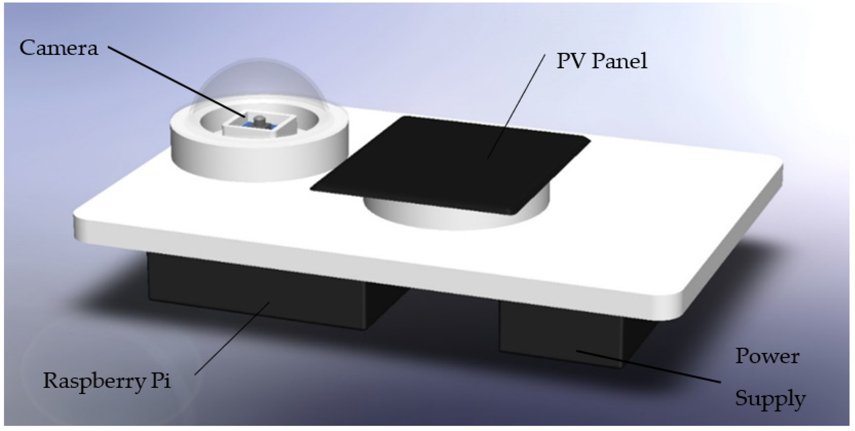
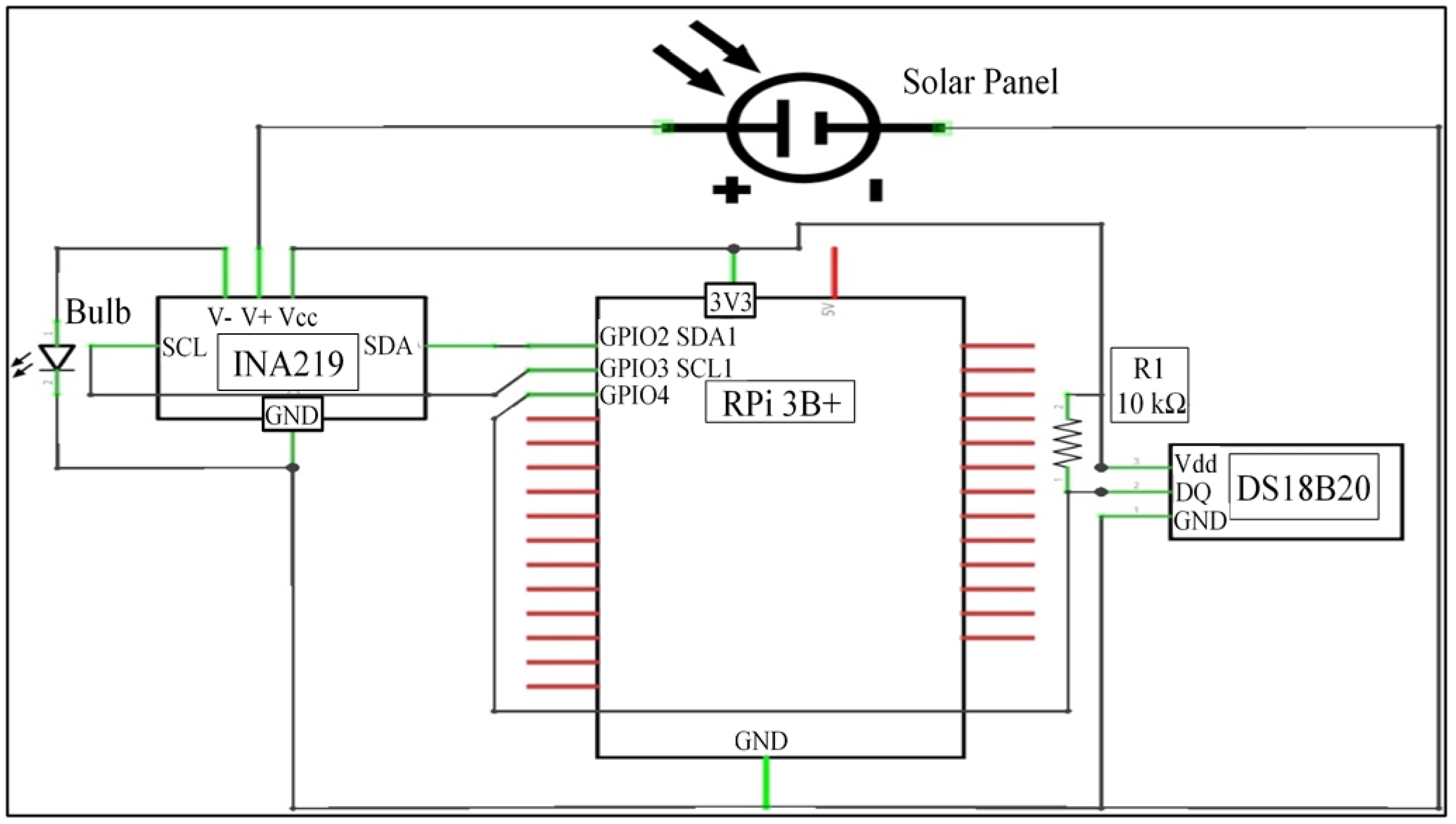
3.1. Data-Acquisition System
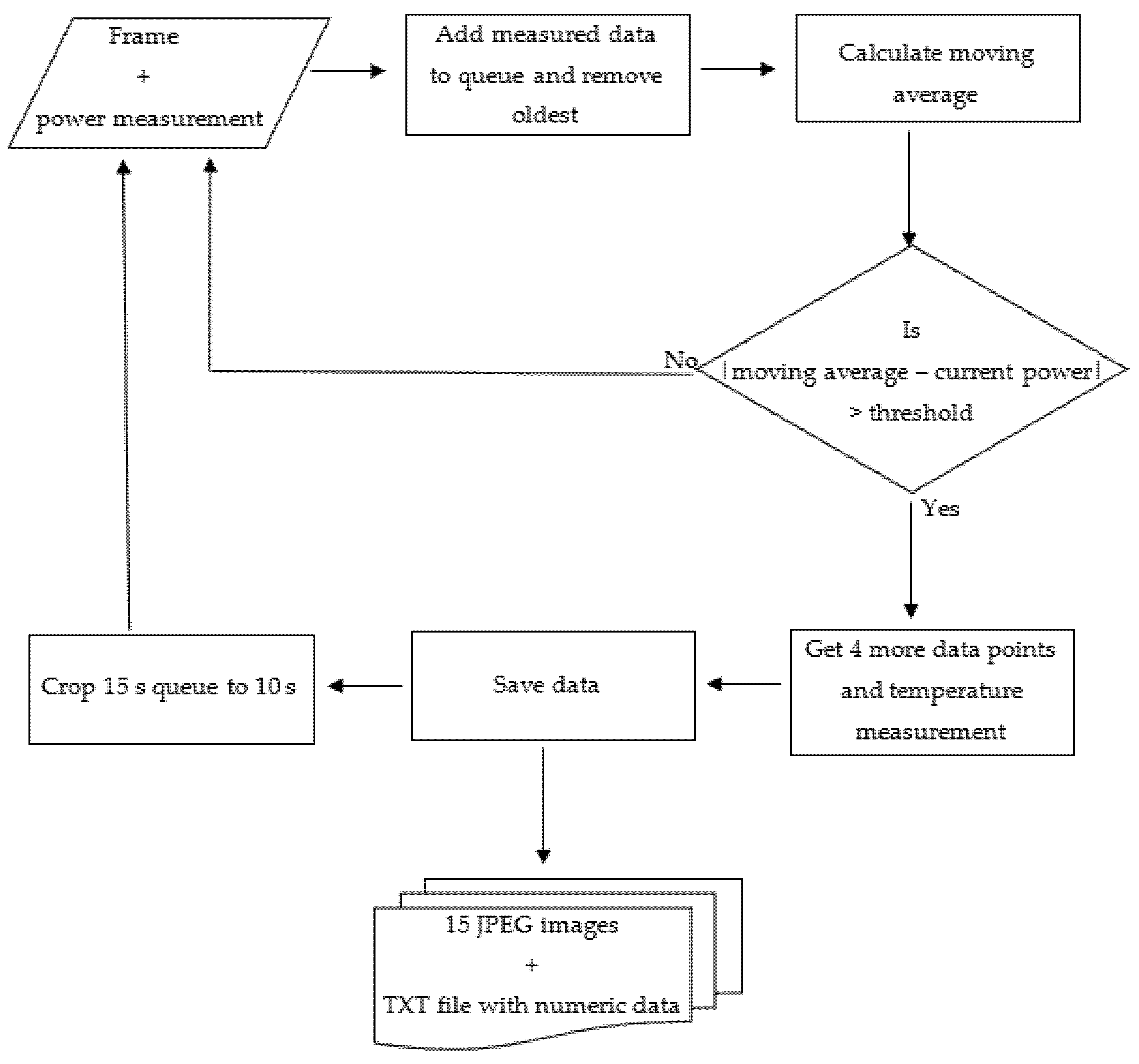
3.2. Acquisition Strategy
3.3. Measured Data
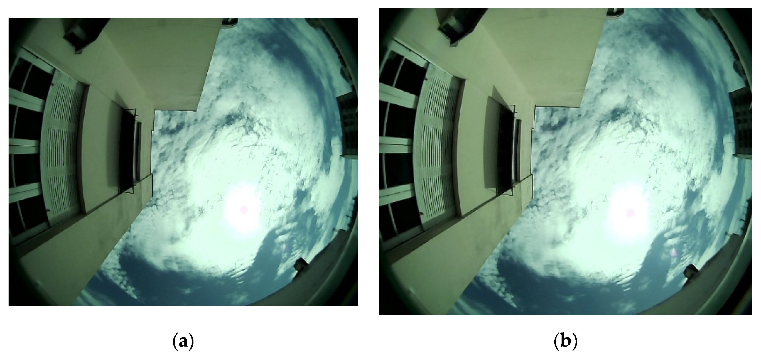
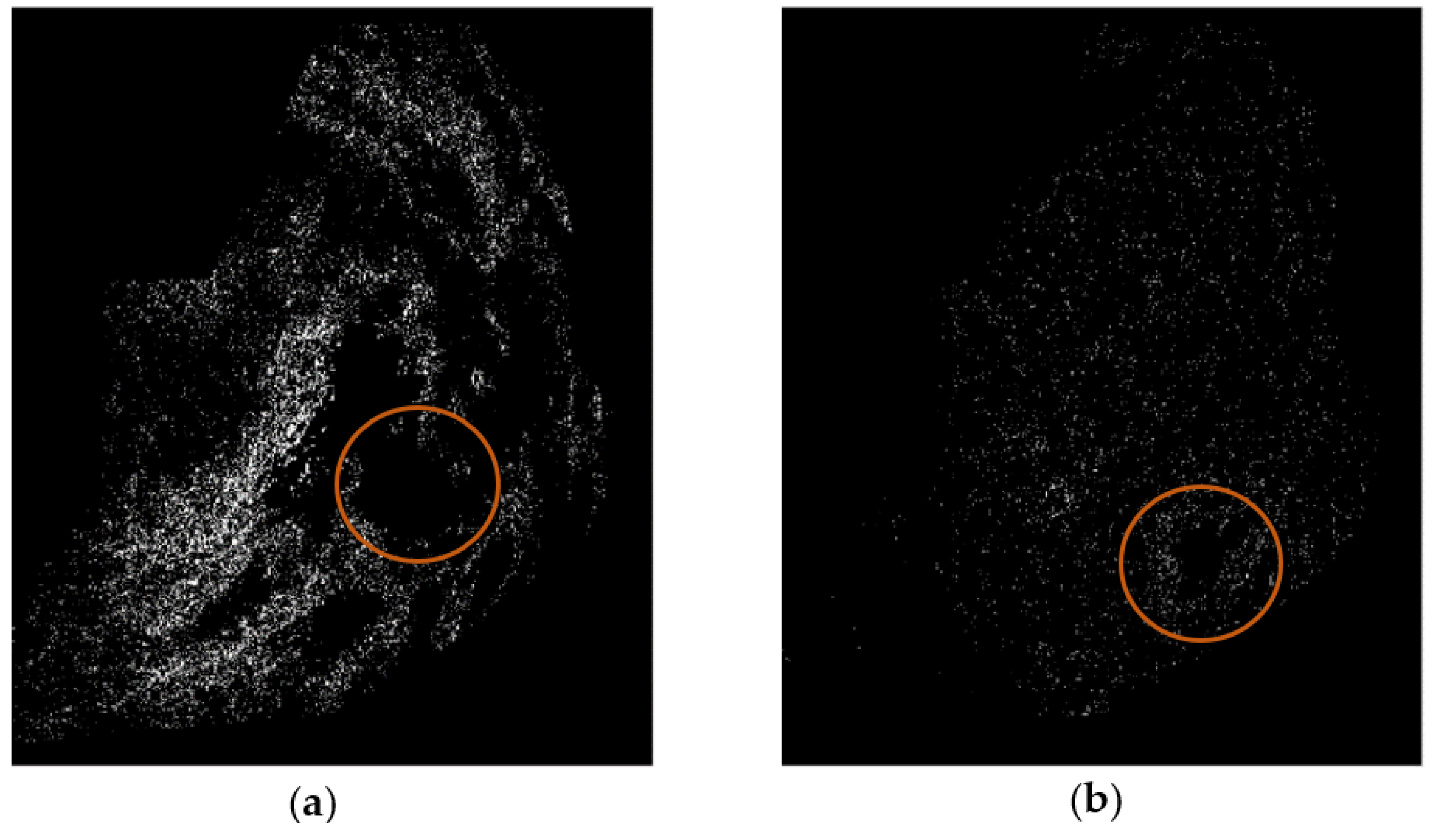
3.4. Visual Analysis
3.5. Correlation Analysis
3.6. Neural Network Modeling
4. Results
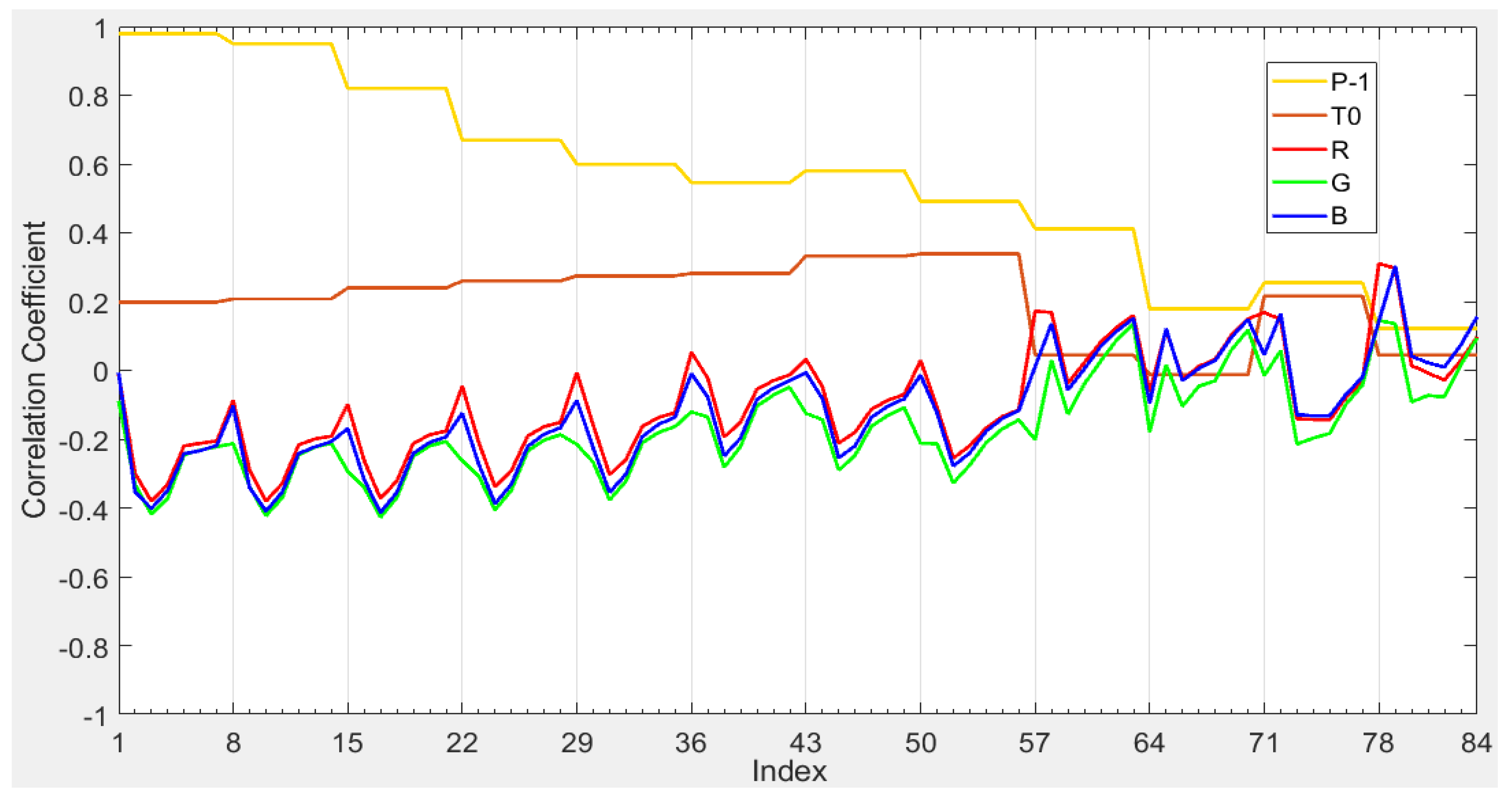
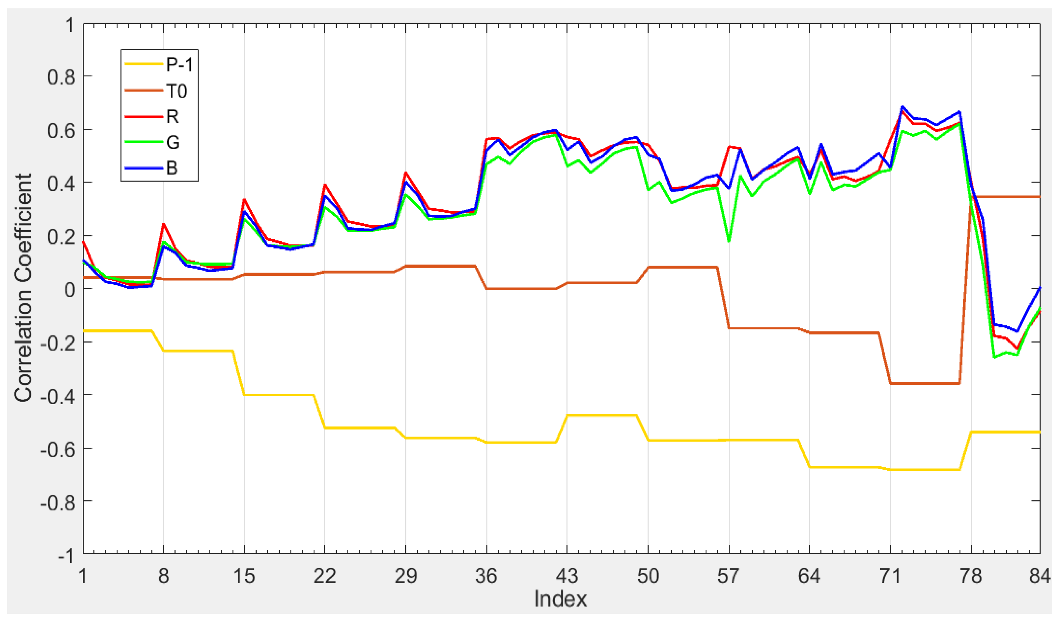
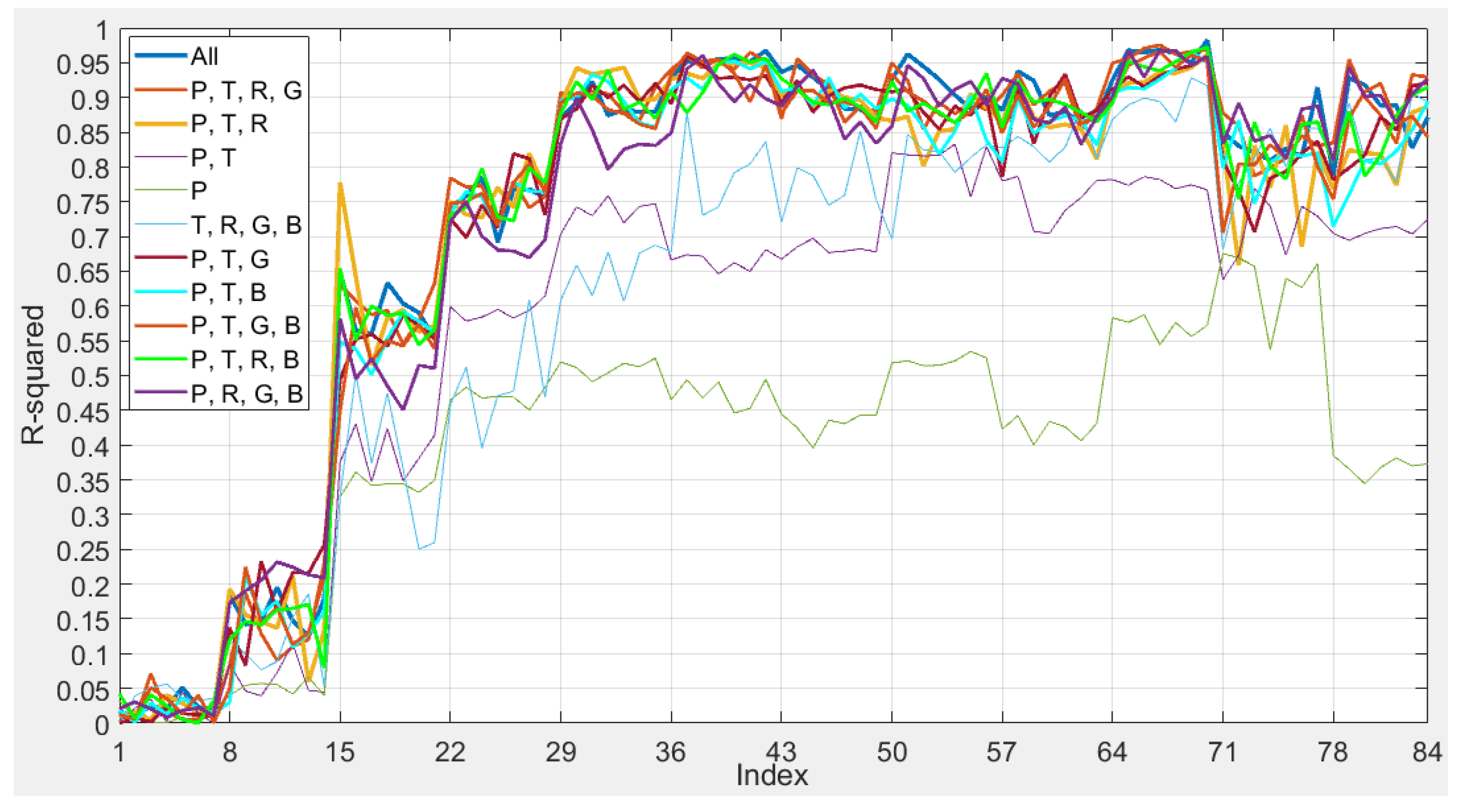
4.1. Correlation Analysis
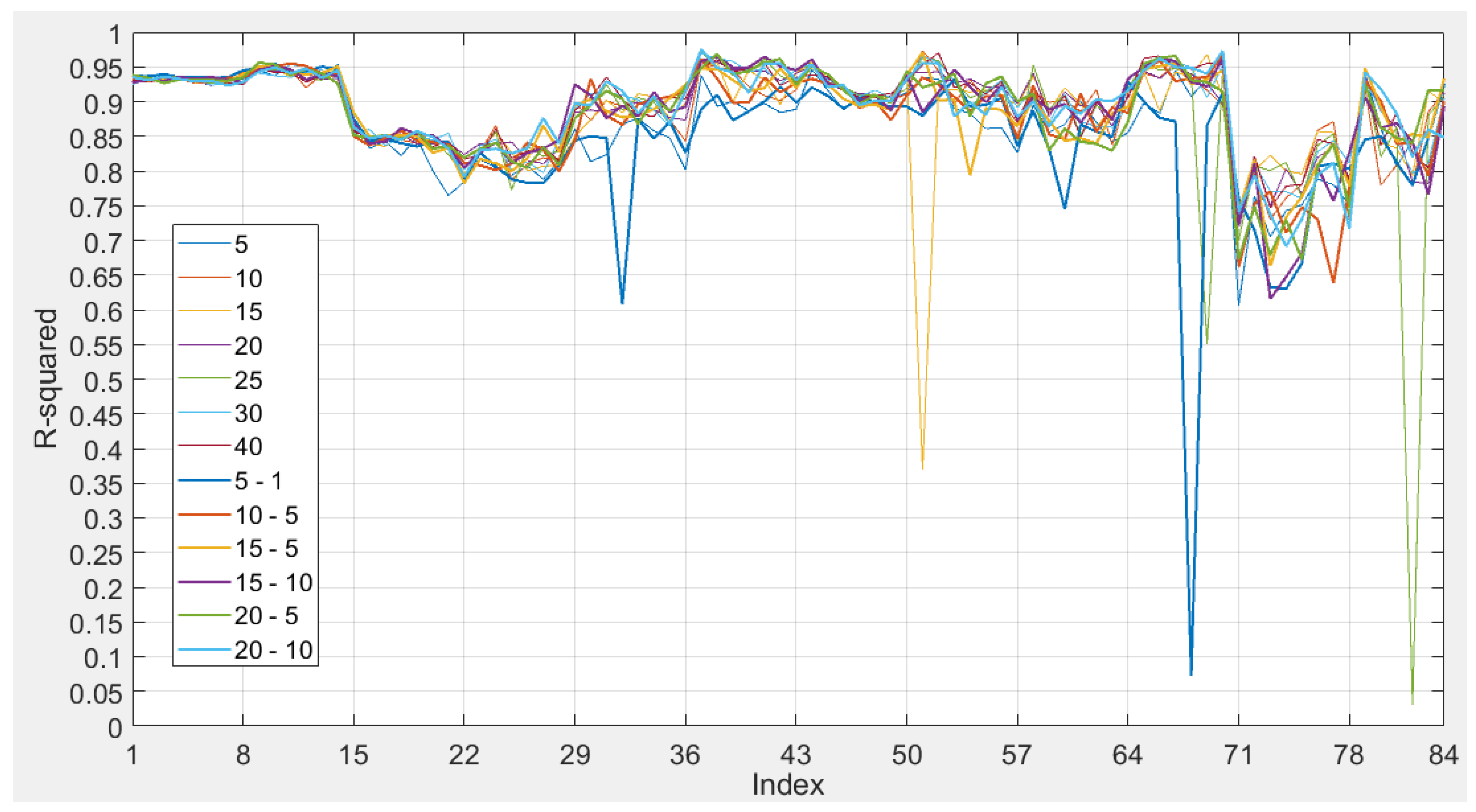
4.2. Neural Network Architecture
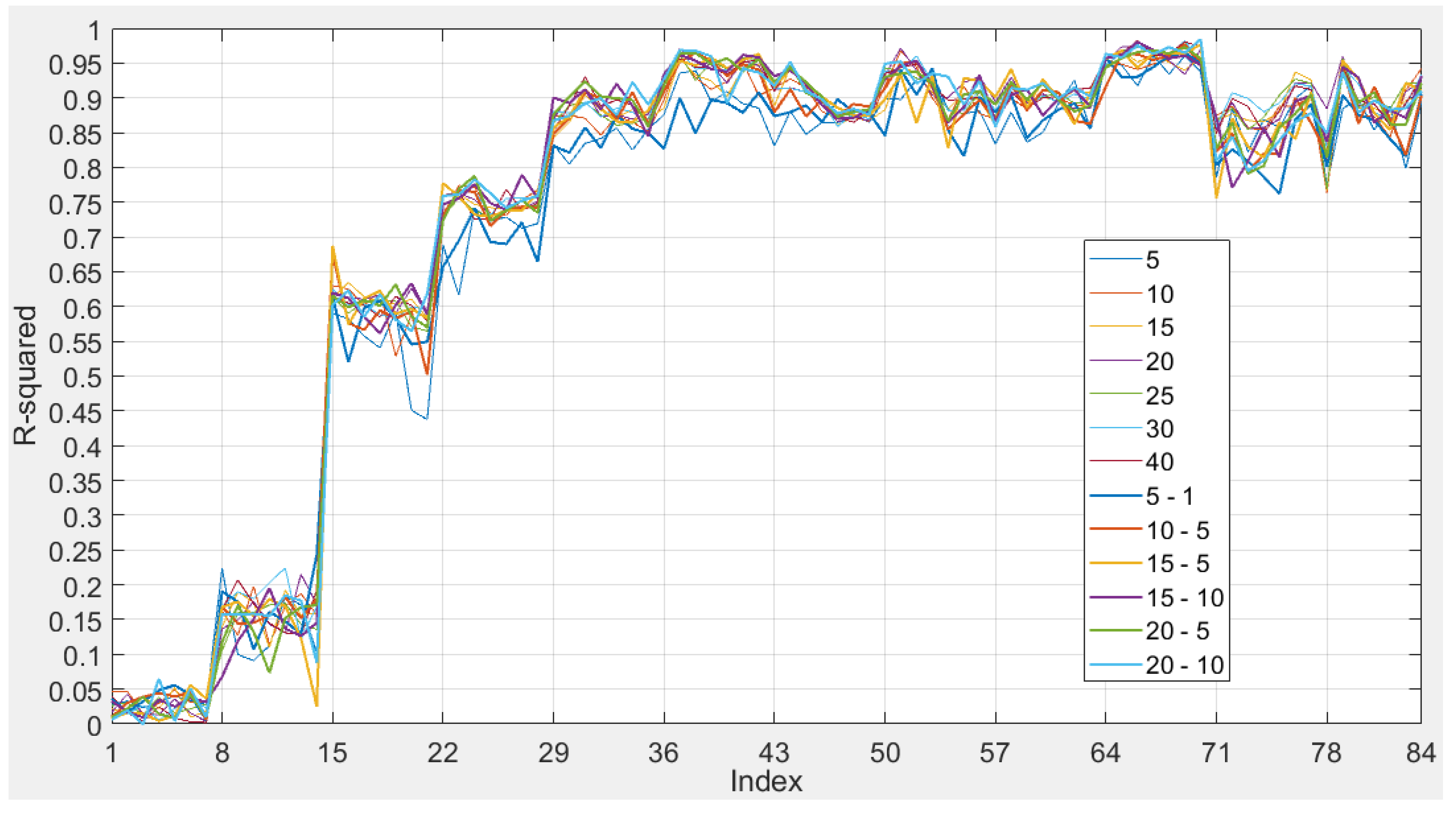
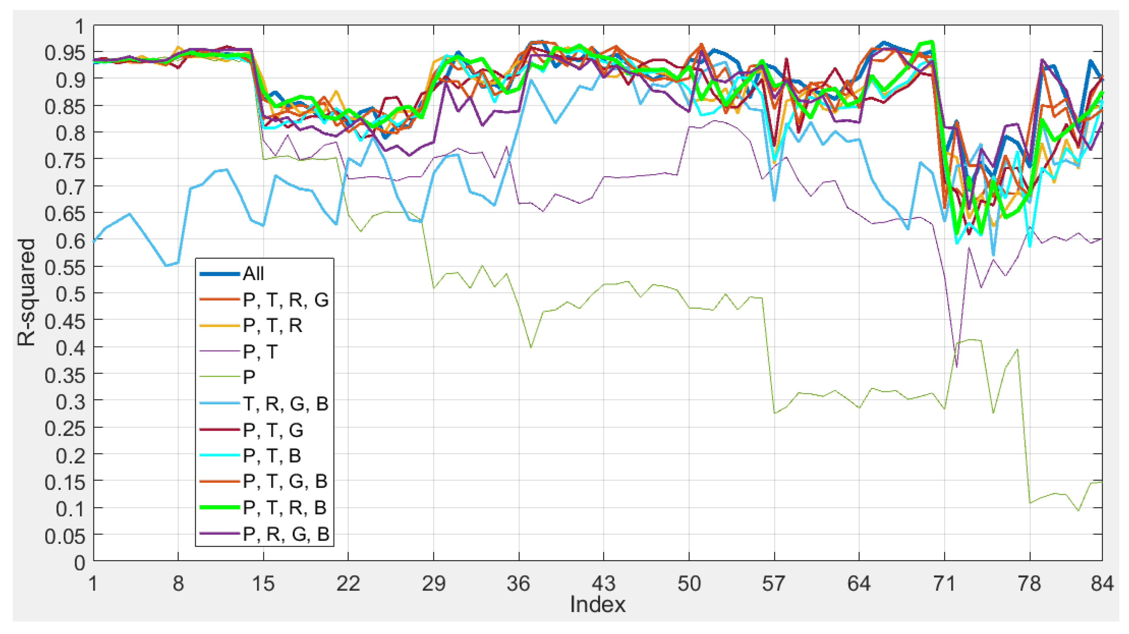
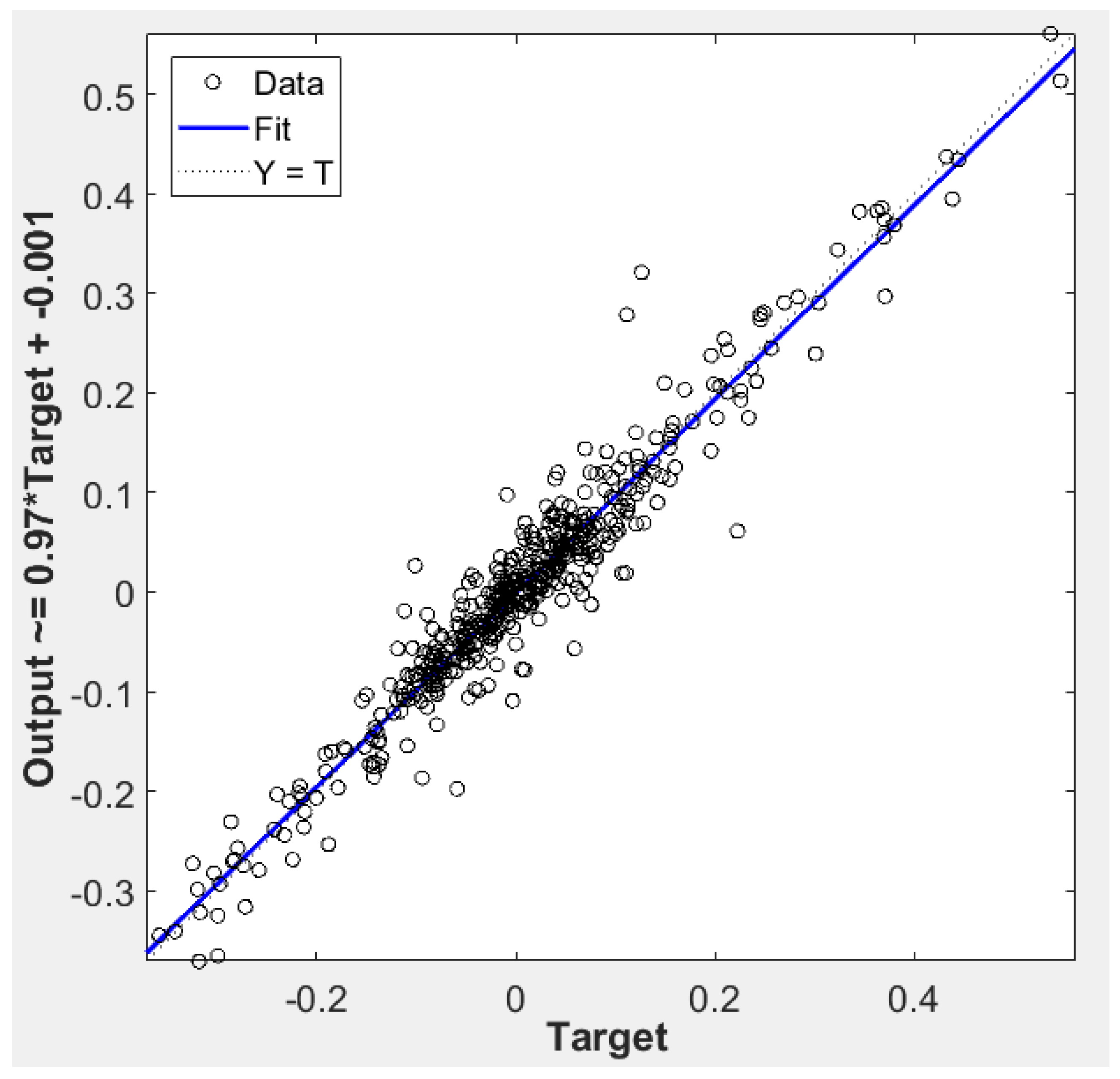
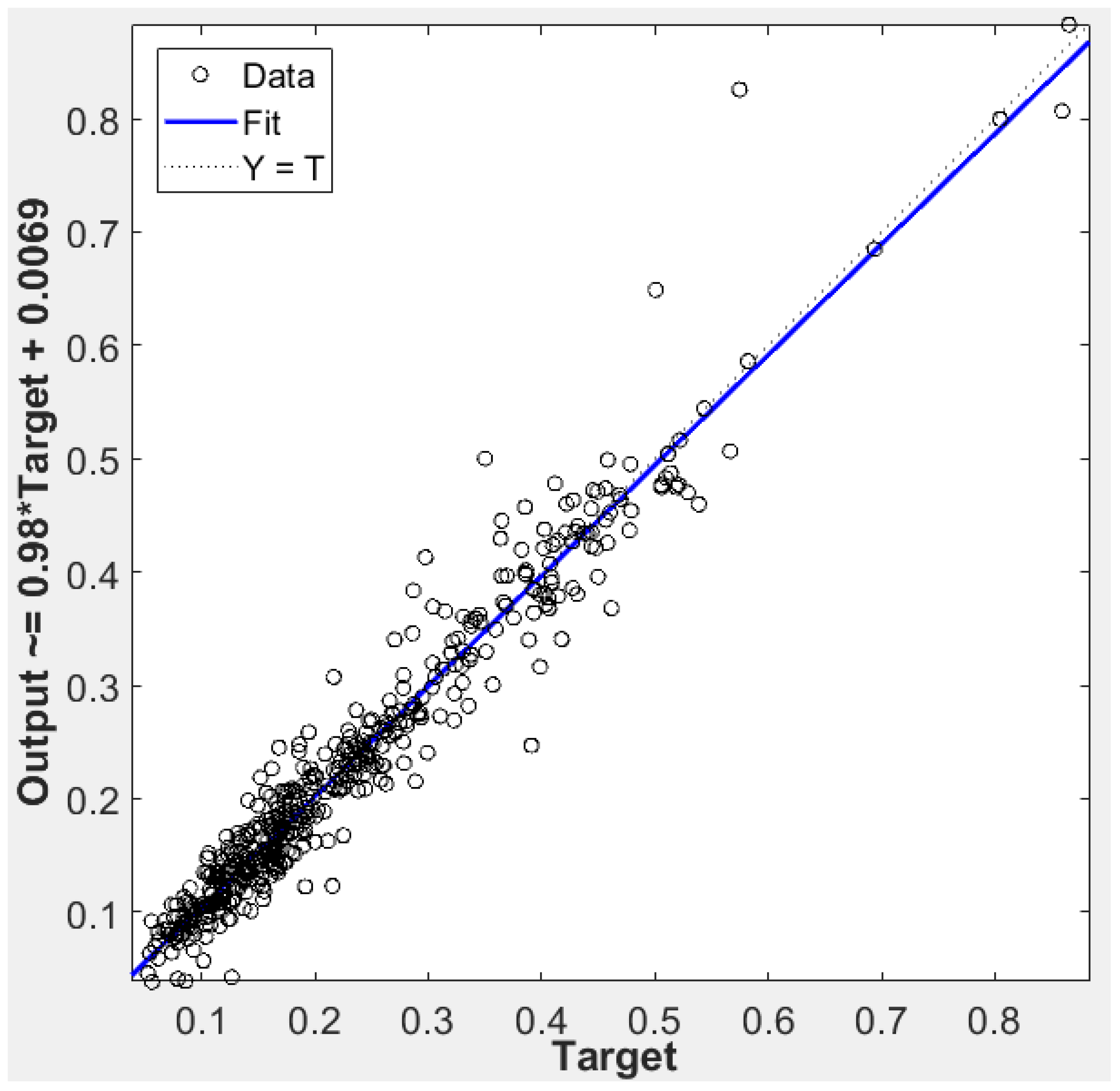
4.3. Best Neural Network Results
4.4. Discussion
5. Conclusions
- Increase geometrical complexity by using arrays of PV panels, mirroring real-world solar farms;
- Test the system in different seasons and climates;
- Couple the model with a cloud tracking and forecast algorithm to provide power forecasts with the system;
- Model the impact of 60 s ahead forecasts for energy-storage management and PV variability mitigation;
- Test the developed acquisition system with the NN model with entirely new data.
Author Contributions
Funding
Institutional Review Board Statement
Informed Consent Statement
Data Availability Statement
Conflicts of Interest
References
- UNFCCC; Paris Agreement: Paris, France, 2015.
- IEA. World Energy Outlook: Executive Summary; IEA: Paris, France, 2018.
- United Nations. Transforming Our World: The 2030 Agenda for Sustainable Development; United Nations: New York, NY, USA, 2015.
- Can Şener, Ş.E.; Sharp, J.L.; Anctil, A. Factors impacting diverging paths of renewable energy: A review. Renew. Sustain. Energy Rev. 2018, 81, 2335–2342. [Google Scholar] [CrossRef]
- Denholm, P.; Margolis, R.M. Evaluating the limits of solar photovoltaics (PV) in traditional electric power systems. Energy Policy 2007, 35, 2852–2861. [Google Scholar] [CrossRef]
- Reddy, S.; Painuly, J.P. Diffusion of renewable energy technologies-barriers and stakeholders’ perspectives. Renew. Energy 2004, 29, 1431–1447. [Google Scholar] [CrossRef]
- Dragoon, K.; Schumaker, A. Solar PV Variability and Grid Integration; Renewable Northwest Project: Portland, OR, USA, 2010. [Google Scholar]
- Mills, A.; Wiser, R. Implications of Wide-Area Geographic Diversity for Short-Term Variability of Solar Power; Lawrence Berkeley National Laboratory: Berkley, MI, USA, 2010. [Google Scholar]
- Bessa, R.; Moreira, C.; Silva, B.; Matos, M. Handling renewable energy variability and uncertainty in power systems operation. Wiley Interdiscip. Rev. Energy Environ. 2014, 3, 156–178. [Google Scholar] [CrossRef]
- Karimi, M.; Mokhlis, H.; Naidu, K.; Uddin, S.; Bakar, A.H.A. Photovoltaic penetration issues and impacts in distribution network—A review. Renew. Sustain. Energy Rev. 2016, 53, 594–605. [Google Scholar] [CrossRef]
- Liang, X. Emerging Power Quality Challenges Due to Integration of Renewable Energy Sources. IEEE Trans. Ind. Appl. 2016, 53, 855–866. [Google Scholar] [CrossRef]
- Diagne, M.; David, M.; Lauret, P.; Boland, J.; Schmutz, N. Review of solar irradiance forecasting methods and a proposition for small-scale insular grids. Renew. Sustain. Energy Rev. 2013, 27, 65–76. [Google Scholar] [CrossRef] [Green Version]
- Sobri, S.; Koohi-Kamali, S.; Rahim, N.A. Solar photovoltaic generation forecasting methods: A review. Energy Convers. Manag. 2018, 156, 459–497. [Google Scholar] [CrossRef]
- Solargis Methodology—Solar Radiation Modeling. Available online: https://solargis.com/docs/methodology/solar-radiation-modeling (accessed on 16 August 2021).
- Natural Earth Countries. Available online: http//www.naturalearthdata.com/download/10m/cultural/ne_10m_admin_0_countries.zip (accessed on 4 June 2020).
- Solargis. Longterm yearly average of global irradiation at optimum tilt. Global Solar Atlas 2019. [Google Scholar]
- United Nations. The Sustainable Development Goals Report; United Nations: New York, NY, USA, 2021.
- Barbieri, F.; Rajakaruna, S.; Ghosh, A. Very short-term photovoltaic power forecasting with cloud modeling: A review. Renew. Sustain. Energy Rev. 2017, 75, 242–263. [Google Scholar] [CrossRef] [Green Version]
- Schmidt, T.; Kalisch, J.; Lorenz, E.; Heinemann, D. Evaluating the spatiooral performance of sky-imager-based solar irradiance analysis and forecasts. Atmos. Chem. Phys. 2016, 16, 3399–3412. [Google Scholar] [CrossRef] [Green Version]
- Kow, K.W.; Wong, Y.W.; Rajkumar, R.; Isa, D. An intelligent real-time power management system with active learning prediction engine for PV grid-tied systems. J. Clean. Prod. 2018, 205, 252–265. [Google Scholar] [CrossRef]
- Denholm, P.; Hand, M. Grid flexibility and storage required to achieve very high penetration of variable renewable electricity. Energy Policy 2011, 39, 1817–1830. [Google Scholar] [CrossRef]
- IEC. Electrical Energy Storage—White Paper. Int. Electrotech. Comm. 2011, 1–78. [Google Scholar] [CrossRef]
- Petinrin, J.O.; Shaabanb, M. Impact of renewable generation on voltage control in distribution systems. Renew. Sustain. Energy Rev. 2016, 65, 770–783. [Google Scholar] [CrossRef]
- Varma, R.K.; Salehi, R. SSR Mitigation with a New Control of PV Solar Farm as STATCOM (PV-STATCOM). IEEE Trans. Sustain. Energy 2017, 8, 1473–1483. [Google Scholar] [CrossRef]
- Richardson, W.; Krishnaswami, H.; Vega, R.; Cervantes, M. A low cost, edge computing, all-sky imager for cloud tracking and intra-hour irradiance forecasting. Sustainability 2017, 9, 482. [Google Scholar] [CrossRef] [Green Version]
- Oliveira, A.; Calili, R.; Almeida, M.F.; Sousa, M. A Systemic and Contextual Framework to Define a Country’s 2030 Agenda from a Foresight Perspective. Sustainability 2019, 11, 6360. [Google Scholar] [CrossRef] [Green Version]
- Bassous, G.F. Development and Validation of a Low-Cost Data Acquisition System for Very Short- Term Photovoltaic Power Forecasting. PUC-Rio 2019. Available online: https://www.maxwell.vrac.puc-rio.br/47953/47953.PDF (accessed on 17 September 2021).
- Stefferud, K.; Kleissl, J.; Schoene, J. Solar forecasting and variability analyses using sky camera cloud detection and motion vectors. In Proceedings of the 2012 IEEE Power and Energy Society General Meeting, San Diego, CA, USA, 22–26 July 2012. [Google Scholar] [CrossRef]
- Reikard, G. Predicting solar radiation at high resolutions: A comparison of time series forecasts. Sol. Energy 2009, 83, 342–349. [Google Scholar] [CrossRef]
- Haykin, S. Neural Networks and Learning Machines: A Comprehensive Foundation, 3rd ed.; Prentice Hall: Upper Saddle River, NJ, USA, 2008; ISBN 9780131471399. [Google Scholar]
- Raza, M.Q.; Nadarajah, M.; Ekanayake, C. On recent advances in PV output power forecast. Sol. Energy 2016, 136, 125–144. [Google Scholar] [CrossRef]
- Das, U.K.; Tey, K.S.; Seyedmahmoudian, M.; Mekhilef, S.; Idris, M.Y.I.; Van Deventer, W.; Horan, B.; Stojcevski, A. Forecasting of photovoltaic power generation and model optimization: A review. Renew. Sustain. Energy Rev. 2018, 81, 912–928. [Google Scholar] [CrossRef]
- Kumler, A.; Xie, Y.; Zhang, Y. A Physics-based Smart Persistence model for Intra-hour forecasting of solar radiation (PSPI) using GHI measurements and a cloud retrieval technique. Sol. Energy 2019, 177, 494–500. [Google Scholar] [CrossRef]
- Zendehboudi, A.; Baseer, M.A.; Saidur, R. Application of support vector machine models for forecasting solar and wind energy resources: A review. J. Clean. Prod. 2018, 199, 272–285. [Google Scholar] [CrossRef]
- Lave, M.; Reno, M.J.; Broderick, R.J. Characterizing local high-frequency solar variability and its impact to distribution studies. Sol. Energy 2015, 118, 327–337. [Google Scholar] [CrossRef]
- Pedro, H.T.C.; Coimbra, C.F.M.; David, M.; Lauret, P. Assessment of machine learning techniques for deterministic and probabilistic intra-hour solar forecasts. Renew. Energy 2018, 123, 191–203. [Google Scholar] [CrossRef]
- Chow, C.W.; Urquhart, B.; Lave, M.; Dominguez, A.; Kleissl, J.; Shields, J.; Washom, B. Intra-hour forecasting with a total sky imager at the UC San Diego solar energy testbed. Sol. Energy 2011, 85, 2881–2893. [Google Scholar] [CrossRef] [Green Version]
- Yang, D.; Kleissl, J.; Gueymard, C.A.; Pedro, H.T.C.; Coimbra, C.F.M. History and trends in solar irradiance and PV power forecasting: A preliminary assessment and review using text mining. Sol. Energy 2018, 168, 60–101. [Google Scholar] [CrossRef]
- Cervantes, M.; Krishnaswami, H.; Richardson, W.; Vega, R. Utilization of Low Cost, Sky-Imaging Technology for Irradiance Forecasting of Distributed Solar Generation. In Proceedings of the 2016 IEEE Green Technologies Conference (GreenTech), Kansas City, MO, USA, 6–8 April 2016; pp. 142–146. [Google Scholar] [CrossRef]
- Urquhart, B.; Kurtz, B.; Dahlin, E.; Ghonima, M.; Shields, J.E.; Kleissl, J. Development of a sky imaging system for short-term solar power forecasting. Atmos. Meas. Tech. 2015, 8, 875–890. [Google Scholar] [CrossRef] [Green Version]
- Gohari, S.M.I.; Urquhart, B.; Yang, H.; Kurtz, B.; Nguyen, D.; Chow, C.W.; Ghonima, M.; Kleissl, J. Comparison of solar power output forecasting performance of the Total Sky Imager and the University of California, San Diego Sky Imager. Energy Procedia 2013, 49, 2340–2350. [Google Scholar] [CrossRef] [Green Version]
- Chu, Y.; Pedro, H.T.C.; Coimbra, C.F.M. Hybrid intra-hour DNI forecasts with sky image processing enhanced by stochastic learning. Sol. Energy 2013, 98, 592–603. [Google Scholar] [CrossRef]
- Marquez, R.; Coimbra, C.F.M. Intra-hour DNI forecasting based on cloud tracking image analysis. Sol. Energy 2013, 91, 327–336. [Google Scholar] [CrossRef]
- Quesada-Ruiz, S.; Chu, Y.; Tovar-Pescador, J.; Pedro, H.T.C.; Coimbra, C.F.M. Cloud-tracking methodology for intra-hour DNI forecasting. Sol. Energy 2014, 102, 267–275. [Google Scholar] [CrossRef]
- West, S.R.; Rowe, D.; Sayeef, S.; Berry, A. Short-term irradiance forecasting using skycams: Motivation and development. Sol. Energy 2014, 110, 188–207. [Google Scholar] [CrossRef]
- Chu, Y.; Pedro, H.T.C.; Li, M.; Coimbra, C.F.M. Real-time forecasting of solar irradiance ramps with smart image processing. Sol. Energy 2015, 114, 91–104. [Google Scholar] [CrossRef]
- Alonso-Montesinos, J.; Batlles, F.J. The use of a sky camera for solar radiation estimation based on digital image processing. Energy 2015, 90, 377–386. [Google Scholar] [CrossRef]
- Alonso-Montesinos, J.; Batlles, F.J.; Portillo, C. Solar irradiance forecasting at one-minute intervals for different sky conditions using sky camera images. Energy Convers. Manag. 2015, 105, 1166–1177. [Google Scholar] [CrossRef]
- Cazorla, A.; Husillos, C.; Antón, M.; Alados-Arboledas, L. Multi-exposure adaptive threshold technique for cloud detection with sky imagers. Sol. Energy 2015, 114, 268–277. [Google Scholar] [CrossRef] [Green Version]
- Chu, Y.; Li, M.; Pedro, H.T.C.; Coimbra, C.F.M. Real-time prediction intervals for intra-hour DNI forecasts. Renew. Energy 2015, 83, 234–244. [Google Scholar] [CrossRef]
- Chu, Y.; Urquhart, B.; Gohari, S.M.I.; Pedro, H.T.C.; Kleissl, J.; Coimbra, C.F.M. Short-term reforecasting of power output from a 48 MWe solar PV plant. Sol. Energy 2015, 112, 68–77. [Google Scholar] [CrossRef]
- Lipperheide, M.; Bosch, J.L.; Kleissl, J. Embedded nowcasting method using cloud speed persistence for a photovoltaic power plant. Sol. Energy 2015, 112, 232–238. [Google Scholar] [CrossRef]
- Pedro, H.T.C.; Coimbra, C.F.M. Nearest-neighbor methodology for prediction of intra-hour global horizontal and direct normal irradiances. Renew. Energy 2015, 80, 770–782. [Google Scholar] [CrossRef]
- Xu, J.; Yoo, S.; Yu, D.; Huang, D.; Heiser, J.; Kalb, P. Solar irradiance forecasting using multi-layer cloud tracking and numerical weather prediction. In Proceedings of the 30th Annual ACM Symposium on Applied Computing—SAC’15, Salamanca, Spain, 13–17 April 2015; ACM Press: New York, NY, USA, 2015; pp. 2225–2230. [Google Scholar]
- Mejia, F.A.; Kurtz, B.; Murray, K.; Hinkelman, L.M.; Sengupta, M.; Xie, Y.; Kleissl, J. Coupling sky images with radiative transfer models: A new method to estimate cloud optical depth. Atmos. Meas. Tech. 2016, 9, 4151–4165. [Google Scholar] [CrossRef] [Green Version]
- Rana, M.; Koprinska, I.; Agelidis, V.G. Univariate and multivariate methods for very short-term solar photovoltaic power forecasting. Energy Convers. Manag. 2016, 121, 380–390. [Google Scholar] [CrossRef]
- Sanfilippo, A.; Martin-Pomares, L.; Mohandes, N.; Perez-Astudillo, D.; Bachour, D. An adaptive multi-modeling approach to solar nowcasting. Sol. Energy 2016, 125, 77–85. [Google Scholar] [CrossRef]
- Soubdhan, T.; Ndong, J.; Ould-Baba, H.; Do, M.-T. A robust forecasting framework based on the Kalman filtering approach with a twofold parameter tuning procedure: Application to solar and photovoltaic prediction. Sol. Energy 2016, 131, 246–259. [Google Scholar] [CrossRef]
- Ai, Y.; Peng, Y.; Wei, W. A model of very short-term solar irradiance forecasting based on low-cost sky images. AIP Conf. Proc. 2017, 1839, 020022. [Google Scholar] [CrossRef] [Green Version]
- Blanc, P.; Massip, P.; Kazantzidis, A.; Tzoumanikas, P.; Kuhn, P.; Wilbert, S.; Schüler, D.; Prahl, C. Short-term forecasting of high resolution local DNI maps with multiple fish-eye cameras in stereoscopic mode. AIP Conf. Proc. 2017, 1850, 140004. [Google Scholar] [CrossRef] [Green Version]
- Cheng, H.Y. Cloud tracking using clusters of feature points for accurate solar irradiance nowcasting. Renew. Energy 2017, 104, 281–289. [Google Scholar] [CrossRef]
- Elsinga, B.; van Sark, W.G.J.H.M. Short-term peer-to-peer solar forecasting in a network of photovoltaic systems. Appl. Energy 2017, 206, 1464–1483. [Google Scholar] [CrossRef]
- Ni, Q.; Zhuang, S.; Sheng, H.; Kang, G.; Xiao, J. An ensemble prediction intervals approach for short-term PV power forecasting. Sol. Energy 2017, 155, 1072–1083. [Google Scholar] [CrossRef]
- Kuhn, P.; Nouri, B.; Wilbert, S.; Prahl, C.; Kozonek, N.; Schmidt, T.; Yasser, Z.; Ramirez, L.; Zarzalejo, L.; Meyer, A.; et al. Validation of an all-sky imager–based nowcasting system for industrial PV plants. Prog. Photovolt. Res. Appl. 2018, 26, 608–621. [Google Scholar] [CrossRef]
- Bouzgou, H.; Gueymard, C.A. Fast short-term global solar irradiance forecasting with wrapper mutual information. Renew. Energy 2019, 133, 1055–1065. [Google Scholar] [CrossRef]
- Chow, C.W.; Belongie, S.; Kleissl, J. Cloud motion and stability estimation for intra-hour solar forecasting. Sol. Energy 2015, 115, 645–655. [Google Scholar] [CrossRef]
- Wood-Bradley, P.; Zapata, J.; Pye, J. Cloud tracking with optical flow for short-term solar forecasting. In Proceedings of the 50th Conference of the Australian Solar Energy Society, Melbourne, VIC, Australia, 21–22 August 2012; pp. 2–7. [Google Scholar]
- Borrill, C.; Timmons, T.; van Staveren, T.; Kluyver, T.; Bauer, S. pi_ina219. Available online: https://github.com/chrisb2/pi_ina219 (accessed on 24 July 2019).
- Furrer, T. w1thermsensor. Available online: https://github.com/timofurrer/w1thermsensor (accessed on 24 July 2019).
- Smets, A.H.; Jäger, K.; Isabella, O.; van Swaaij, R.A.; Zeman, M. Solar Energy: The Physics and Engineering of Photovoltaic Conversion, Technologies and Systems, 1st ed.; UIT Cambridge Ltd.: Cambrige, UK, 2016; ISBN 978-1906860325. [Google Scholar]
- Amelink, H.; Hoffmann, A.G. Current trends in control centre design. Int. J. Electr. Power Energy Syst. 1983, 5, 205–211. [Google Scholar] [CrossRef]
- Bassous, G.F.; Hall, C.; Calili, R. Sky Images and PV Measurements. Mendeley Data. 2021. Available online: https://data.mendeley.com/datasets/r83r6g5y6t/1 (accessed on 17 September 2021). [CrossRef]


| Category | Time Horizon | Resolution | Applicability |
|---|---|---|---|
| Very short-term | Up to 15 min ahead | Up to 1 min | Plant operation Ramping events Power quality control |
| Short-term | 15 min to 1 h ahead | 1 to 5 min | Load following Grid operation planning |
| Medium-term | 1 h to 6 h | Hourly | Load following Grid operation planning |
| Long-term | One day ahead | Hourly | Unit commitment Transmission scheduling Day ahead markets |
| Work | Objective | Materials and Methods |
|---|---|---|
| Chow et al. (2011) [37] | Forecast of GHI from 30 s to 5 min ahead | Sky images obtained from a Total Sky Imager (TSI) every 30 s; Clear Sky Library (CSL) + Sunshine Parameter + Red-Blue Ratio (RBR) cloud classification; Cloud tracking through cross-correlationGHI deterministically calculated. |
| Gohari et al. (2013) [41] | Forecast of Clear Sky Index up to 15 min ahead in 30 s intervals | Comparison between TSI and UCSD-developed USI; Sky images every 30 s + irradiance measurements every second; Geometric cloud tracking; Solar ray tracing. |
| Chu et al. (2013) [42] | Forecast of 1-min-average DNI 5 min and 10 min ahead | TSI images every 20 s + DNI every 30 s; CLS + RBR adaptive threshold cloud classification; Cloudiness indices from gridded image + time lagged DNI as inputs for NN. |
| Marquez and Coimbra (2013) [43] | Forecast of 1-min-average DNI 3 min to 15 min ahead | TSI images every minute + 30 s averaged DNI; Cloud tracking, using Particle Image Velocimetry software; Hybrid threshold algorithm for cloud pixel classification; Grid of cloudiness indices used to deterministically calculate DNI. |
| Quesada-Ruiz et al. (2014) [44] | Forecast of 1-min-average DNI from 3 to 20 min ahead | TSI images every 20 s + 1 min averaged DNI; Hybrid threshold algorithm for cloud pixel classification; Cloud tracking, using grid cloud fraction change; DNI estimation, using grid cloud fraction. |
| West et al. (2014) [45] | Forecast of DNI from 0 to 20 min ahead in 10 s resolution and updated every 10 s | Sky images from internet protocol (IP) camera + DNI every 10 s; Cloud pixel detection, using NN; Cloud tracking through pixel-wise optical flow; Image regions averaged and total cloudiness as feature to be forecasted and derived into DNI. |
| Chu et al. (2015a) [46] | Forecast of 10 min ahead GHI and DNI | Images from 2 IP sky cameras every 60 s + irradiance every 30 s; Adaptive threshold cloud detection; Gridded cloudiness + time lagged irradiance as inputs for NN. |
| Alonso-Montesinos and Battles (2015) [47] | Modeling of GHI, DNI and DIF | TSI images every 60 s + GHI + DNI every 60 s; Correlations of digital image channels to model irradiance. |
| Alonso-Montesinos et al. (2015) [48] | Forecast of GHI, DNI and DIF from 1 to 180 min, at 15 min resolution | TSI images every 60 s; Cloud tracking, using cloud motion vectors (CMV); Pixel-wise cloud detection;Pixel-wise irradiance, using correlation of digital channel information. |
| Cazorla et al. (2015) [49] | Methodology for cloud detection | SONA sky imager + GHI + DIF; Multi-exposure (High Dynamic Range—HDR) images every 5 min; Adaptive RBR threshold method for cloud detection. |
| Chu et al. (2015) [50] | Forecasting of prediction interval for 1-min-average DNI 5, 10, 15 and 20 min ahead | USI images provide parameters for hybrid model; Hybrid estimation/forecast model based on bootstrapped-ANN selected by SVM classifier, using mean RBR, RBR standard deviation and entropy + time-lagged DNI and DIF measurements as inputs; SVM for sky classification and model selection (high vs. low cloud-derived variability). |
| Chu et al. (2015b) [51] | Forecast of PV power 5, 10 and 15 min ahead | 2 TSI providing images every 30 s; 3 methods as inputs for ANN reforecasting (deterministic based on cloud tracking, ARMA and kNN); Preliminary forecast by one of the 3 methods followed by reforecast, using ANN to enhance performance; Genetic algorithm to select ANN inputs; among several time-lagged power measurements and preliminary power forecasts for each of the horizons. |
| Lipperheide et al. (2015) [52] | Forecast of power ramp events 20 s to 180 s ahead with 20 s resolution | 1 Hz power data from PV panels used in 4 different methods; Persistence and ramp persistence forecast based on detection from PV panels within plant; Cloud speed persistence forecast based on cloud motion vectors detected by PV panel power fluctuation;Second-order autoregressive forecast model based on the modified covariance method. |
| Pedro and Coimbra (2015) [53] | Forecast of GHI and DNI from 5 to 30 min ahead | 5-min-averaged irradiance data; IP camera images every 60 s; Digital image channel individual information and relationships’ properties, such as mean, standard deviation and entropy; kNN forecast model with images vs. without images vs. persistence. |
| Xu et al. (2015) [54] | Forecast of GHI from 1 to 15 min ahead | TSI images every 20 s; Complex cloud detection and tracking; Pixel-wise classification using RGB values, RBR and Laplacian of Gaussian (LoG); Cloud-type classification through texture metrics and kNN classifier; Comparison of persistence, linear regression and Support Vector Regression (SVR) with image inputs and NWP variables. |
| Cervantes et al. (2016) [39] | Forecast of 5 min ahead DNI negative ramp events | Low-cost sky-imager; Cloud detection through RBR; Cloud tracking with optical flow; Shadow mapping, using Cloud Base Height (CBH) data. |
| Mejia et al. (2016) [55] | Cloud optical depth modeling | 2 USI providing images every 30 s; Estimation of irradiance from calibrated pixel values; Usage of deterministic models to obtain optical depth from digital image channels, solar position, pixel position and clear-sky library. |
| Rana et al. (2016) [56] | Forecast of PV power from 5 to 60 min ahead, with 5 min resolution | 5 min power average + meteorological data; Univariate (solely power measurements) vs. multivariate models NN ensemble vs. SVR vs. persistence. |
| Sanfilippo et al. (2016) [57] | Forecast of 1-min-average clearness index from 1 to 15 min ahead | GHI, DNI and DHI measurements every 60 s; Modeling of solar zenith-independent clearness index; SVR, persistence and autoregressive models of different orders used for forecasting. |
| Schmidt et al. (2016) [19] | Forecasts of GHI from 15 s to 25 min GHI forecasts in grid form for the surrounding area, updated every 15 s with 15 s resolution | Sky images every 15 s from custom imager + GHI every 1 s from 99 pyranometers + CBH measurements averaged over 10 min; Area of study of 10 km × 12 km; RBR with clear-sky images for cloud pixel classification; SVC cloud type classification from several features;CMV cloud tracking. |
| Soubdhan et al. (2016) [58] | Forecast of PV power and GHI 1, 5, 10, 30 and 60 min ahead | PV power data every 1 s + percentage cloud cover + ambient temperature + GHI every 1 s; Persistence and smart persistence baselines; Forecasting by Kalman filter with initialized parameters, using expectation-maximization (EM) algorithm vs. autoregressive (AR) estimation; Comparison between with and without exogenous inputs. |
| Ai et al. (2017) [59] | Forecast of 30-s-average GHI 1, 2, 3 min ahead | Sky images every 30 s from IP camera; SVM-determined clear-sky model; Adaptive threshold cloud detection; Optical flow cloud tracking; GHI deterministically determined, using cloud fraction and clear-sky model. |
| Blanc et al. (2017) [60] | Forecast of 1-min-average DNI map 15 min ahead with up to 10 m × 10 m spatial resolution | Stereoscopic IP sky cameras providing images every 30 s; CBH estimation from stereography; Cloud-layer CMV for each class of altitude; Estimation of projection-pixel-wise DNI, using beam clear-sky indexes computed per class of cloud combined with physical and geometrical information. |
| Cheng (2017) [61] | Detection of irradiance ramp down events 5, 10, 15 and 20 min ahead | Sky images every 60 s from Santa Barbara; Instrument Group + 1 min averaged GHI; Cloud detection and tracking through feature point clusters. |
| Elsinga and Van Sark (2017) [62] | Forecasts of 1 min average GHI from 1 to 30 min ahead for multiple sites | 202 rooftop PV systems acting as a sensor grid;PV power data averaged every 1 min from inverter data every 2 s and then converted into GHI; Hourly interpolated ambient temperature deterministically calculated; GHI converted into clearness index Peer-to-Peer (P2P) forecasting method, using correlations between the rooftop PV systems to determine time lag between correlated sites. |
| Ni et al. (2017) [63] | Forecast of power interval 5 min ahead | Ensemble of single-layer feed-forward NN (weights assigned, using a least-squares method in 1 step); Data from 3 kW micro-grid with 3 PV systems + photosynthetically active radiation + ambient temperature + relative humidity + wind speed + wind direction + GHI and precipitation (all averaged over 5 min). |
| Richardson et al. (2017) [25] | Forecast of GHI 10 and 15 min ahead | Images from a PiCamera; Cloud detection, using RBR; Optical flow cloud tracking; Ray tracing for GHI forecast, using a fixed ramp rate and clear sky GHI. |
| Kow et al. (2018) [20] | Forecast of PV power 30 s ahead coupled with mitigation system | GHI every 1 s + ambient temperature every 1 s and PV system modeled power; Self-organizing incremental neural network (M-SOINN) with active learning for forecasting power; Non-supervised method capable of forecasting power output of PV system 30 s ahead. |
| Kuhn et al. (2018) [64] | Forecast of 1-min-average GHI from 0 to 15 min ahead | Cloud segmentation, detection and georeferencing, using 4 sky cameras (WobaS-4cam) and 4-dimensional CSL; Irradiance maps validated with ground irradiance sensors and shadow camera; GHI and DNI obtained from geo-located shadow map and radiometer measurements at previous time steps. |
| Bouzgou and Gueymard (2019) [65] | Forecast of GHI from 5 min to 3 h ahead | Mutual information feature selection from time series of recent GHI; Extreme learning machine (ELM) for investigating the relationship between the historical variables and the future value, and also for determining the best combination of variables. |
| Kumler et al. (2019) [33] | Forecast of GHI 5, 15, 30 and 60 min ahead | Cloud albedo and fraction modeling based on GHI; Cloud optical thickness deterministically calculated; Forecast based on 5 min exponential weighed moving average of cloud fraction, used to determine albedo and GHI. |
| Time Stamp | Temperature (°C) | Voltage (V) | Current (A) | Power (W) |
|---|---|---|---|---|
| 12_27_34_2019_03_17_0 | 48.0 | 0.241 | 0.614 | 0.148 |
| 12_27_33_2019_03_17_0 | −1000 | 0.246 | 0.626 | 0.154 |
| 12_27_32_2019_03_17_0 | −1000 | 0.251 | 0.632 | 0.158 |
| 12_27_31_2019_03_17_0 | −1000 | 0.247 | 0.633 | 0.156 |
| 12_27_30_2019_03_17_0 | −1000 | 0.246 | 0.629 | 0.155 |
| 12_27_29_2019_03_17_0 | −1000 | 0.242 | 0.621 | 0.150 |
| 12_27_28_2019_03_17_0 | −1000 | 0.236 | 0.609 | 0.144 |
| 12_27_27_2019_03_17_0 | −1000 | 0.232 | 0.601 | 0.139 |
| 12_27_26_2019_03_17_0 | −1000 | 0.227 | 0.595 | 0.135 |
| 12_27_25_2019_03_17_0 | −1000 | 0.226 | 0.589 | 0.133 |
| 12_27_24_2019_03_17_0 | 48.0 | 0.222 | 0.584 | 0.130 |
| 12_27_23_2019_03_17_0 | −1000 | 0.222 | 0.581 | 0.129 |
| 12_27_22_2019_03_17_0 | −1000 | 0.217 | 0.576 | 0.125 |
| 12_27_21_2019_03_17_0 | −1000 | 0.216 | 0.569 | 0.123 |
| 12_27_20_2019_03_17_0 | −1000 | 0.212 | 0.561 | 0.119 |
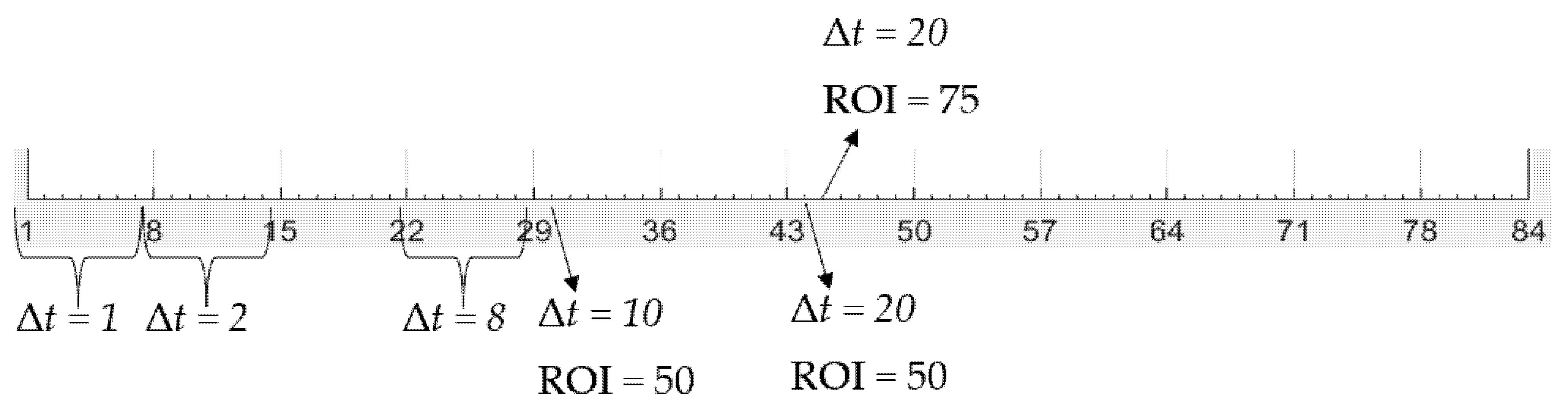
| ROI Radius (pixels) | Δt (s) | |||||||||||
|---|---|---|---|---|---|---|---|---|---|---|---|---|
| 1 | 2 | 5 | 8 | 10 | 15 | 20 | 30 | 45 | 60 | 75 | 90 | |
| 25 | 1 | 8 | 15 | 22 | 29 | 36 | 43 | 50 | 57 | 64 | 71 | 78 |
| 50 | 2 | 9 | 16 | 23 | 30 | 37 | 44 | 51 | 58 | 65 | 72 | 79 |
| 75 | 3 | 10 | 17 | 24 | 31 | 38 | 45 | 52 | 59 | 66 | 73 | 80 |
| 100 | 4 | 11 | 18 | 25 | 32 | 39 | 46 | 53 | 60 | 67 | 74 | 81 |
| 150 | 5 | 12 | 19 | 26 | 33 | 40 | 47 | 54 | 61 | 68 | 75 | 82 |
| 200 | 6 | 13 | 20 | 27 | 34 | 41 | 48 | 55 | 62 | 69 | 76 | 83 |
| 250 | 7 | 14 | 21 | 28 | 35 | 42 | 49 | 56 | 63 | 70 | 77 | 84 |
| Model | Variables | ||||
|---|---|---|---|---|---|
| P−1 | T0 | R | G | B | |
| 1 | X | X | X | X | X |
| 2 | X | X | X | X | O |
| 3 | X | X | X | O | O |
| 4 | X | X | O | O | O |
| 5 | X | O | O | O | O |
| 6 | O | X | X | X | X |
| 7 | X | X | O | X | O |
| 8 | X | X | O | O | X |
| 9 | X | X | O | X | X |
| 10 | X | X | X | O | X |
| 11 | X | O | X | X | X |
Publisher’s Note: MDPI stays neutral with regard to jurisdictional claims in published maps and institutional affiliations. |
© 2021 by the authors. Licensee MDPI, Basel, Switzerland. This article is an open access article distributed under the terms and conditions of the Creative Commons Attribution (CC BY) license (https://creativecommons.org/licenses/by/4.0/).
Share and Cite
Bassous, G.F.; Calili, R.F.; Barbosa, C.H. Development of a Low-Cost Data Acquisition System for Very Short-Term Photovoltaic Power Forecasting. Energies 2021, 14, 6075. https://doi.org/10.3390/en14196075
Bassous GF, Calili RF, Barbosa CH. Development of a Low-Cost Data Acquisition System for Very Short-Term Photovoltaic Power Forecasting. Energies. 2021; 14(19):6075. https://doi.org/10.3390/en14196075
Chicago/Turabian StyleBassous, Guilherme Fonseca, Rodrigo Flora Calili, and Carlos Hall Barbosa. 2021. "Development of a Low-Cost Data Acquisition System for Very Short-Term Photovoltaic Power Forecasting" Energies 14, no. 19: 6075. https://doi.org/10.3390/en14196075
APA StyleBassous, G. F., Calili, R. F., & Barbosa, C. H. (2021). Development of a Low-Cost Data Acquisition System for Very Short-Term Photovoltaic Power Forecasting. Energies, 14(19), 6075. https://doi.org/10.3390/en14196075