The Icing Distribution Characteristics Research of Tower Cross Beam of Long-Span Bridge by Numerical Simulation

Abstract

The cross beam of a long-span bridge will freeze in low temperature. When the temperature rises, the ice on the cross beam will thaw and fall off. If the ice is too heavy, it may cause vehicle damage and casualty. In order to reduce the risk of falling ice, a scale model of the cross beam was taken as an example, and a kind of numerical simulation method is presented to study the icing distribution characteristics on surface of the cross beam. This paper simulates the ice accretions process of the cross beam by Fluent module and FENSAP-ICE module of ANSYS and investigates the influence of wind and temperature in the process. This is a new numerical simulation method for studying ice accretions of buildings. The results indicate that water freezes mainly on the windward surface, and the thicker ice is near the top and bottom edge of windward surface. According to the results of numerical simulation, a measure of ice melting based on electric heating method is proposed in this paper, and the feasibility and effectiveness of this method are verified by numerical simulation. The results show that the icing distribution characteristics are accord with the fact and the ice-melting measure is feasible and effective.

1. Introduction

Low temperature can cause ice accretions of bridge structures, and when temperature rises, the ice will thaw and fall off. Some bridges, such as Erqi Yangtze River Bridge in Wuhan City, Hubei Province, experienced large-scale ice shedding during winter warming. Falling ice mostly occurs in long-span, cable-stayed bridges and suspension bridges. When the temperature is low, fog, rain, and snow may condense on the cross beam and cable of the bridge tower to form ice and thicken it continuously, which will cause damage to the cable structure and affects the safety and stability of the bridge [1]. At the same time, the ice may fall into the road under the action of gravity when it is melting [2], which brings huge security risks to traffic. Due to the large area of the tower cross beam of long-span bridges, once the beam begins to freeze, it is easy for water to adhere to the beam and form a large ice mass. The risk caused by such ice shedding is greater. Therefore, it is necessary to take prevention measures against falling ice to ensure the traffic safety of bridges in low temperature.

At present, the research on snow and ice melting of bridges in the world mainly focus on pavement of bridges. Some researchers have proposed geothermal methods, conductive concrete methods, and electric heating methods to melt snow and ice on the road. Geothermal methods are to embed or attach pipes on the road and use gas or liquid as a circulating medium to transfer geothermal energy from the ground to the road for snow and ice melting [3,4,5,6,7,8]. However, the construction and installation of geothermal energy mining equipment is very complex, and due to the limitation of geothermal conditions, it is possible to exploit geothermal energy in the plateau area 100 m deep underground [9]. Conductive concrete methods are to mix the appropriate amount of steel fiber [10], carbon fiber [11,12] or graphene into concrete [13]; in this way, the concrete can have a certain electrical resistance so that the concrete can produce heat to melt ice and snow after being electrified. However, the doped materials are prone to corrosion in concrete, resulting in the decrease of electrical and thermal efficiency [14]. Moreover, it is difficult for the admixture in concrete to be uniformly distributed, which affects the conductivity. Electric heating methods include laying carbon nanotubes [15] and carbon fiber heating line [16] under pavement, using the electrothermal properties of these materials to heat the road to melt snow and ice [17]. In order to improve the efficiency of snow and ice melting, researchers studied the influence of heating material layout, electric power, and environmental factors on the efficiency of snow and ice melting [18,19,20]. As for other bridge structures, researchers pay more attention to the effects of ice accretion on the aerodynamics of bridge structures; the results of their experiments show that the ice accretion can obviously increase the wind-induced response of bridge structures, which will deteriorate the wind-resistant performance of bridges [21,22,23,24] and even cause catastrophic failure to bridges [25]. Research on snow and ice melting of the cross beam of the bridge tower are fewer. At present, manual clearing and mechanical clearing are still mainly used to melt snow and ice on the bridge cables and cross beam, and the efficiency is low. Especially for cable-stayed bridges with large spans, manual de-icing and mechanical de-icing have high cost, low efficiency, and poor effect.

In order to promote the solution of the ice-falling problem of the bridge tower cross beam, the current study simulates the icing situation of the cross beam through the Fluent module and FENSAP-ICE module of ANSYS. According to the results of the simulation test, this paper proposes to use heating modules to melt the ice on the cross beam and studies the influence of arranging heating modules to the ice distributions on cross beam. Finally, some advice about finding the appropriate places on the cross beam to set heating modules and raising the efficiency of melting ice are proposed.

2. Study on the Influence of Wind and Temperature on the Icing Simulation Results of Cross Beam

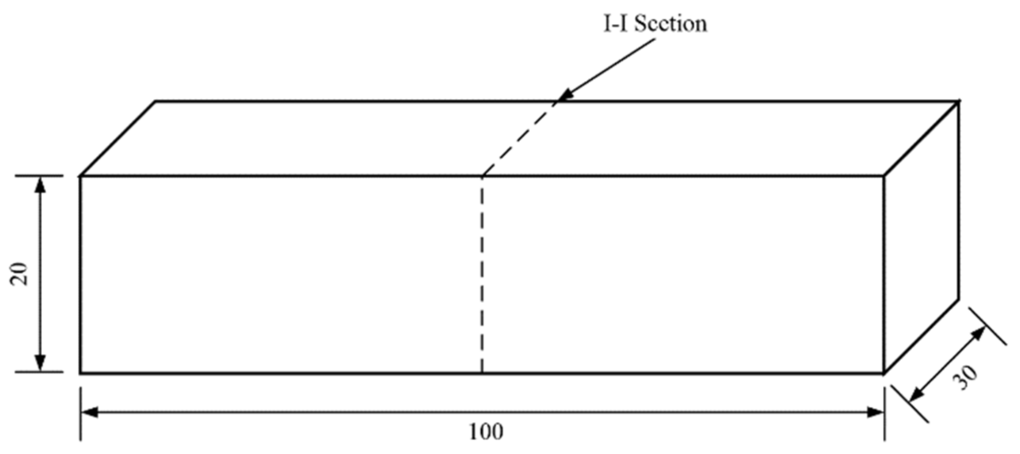
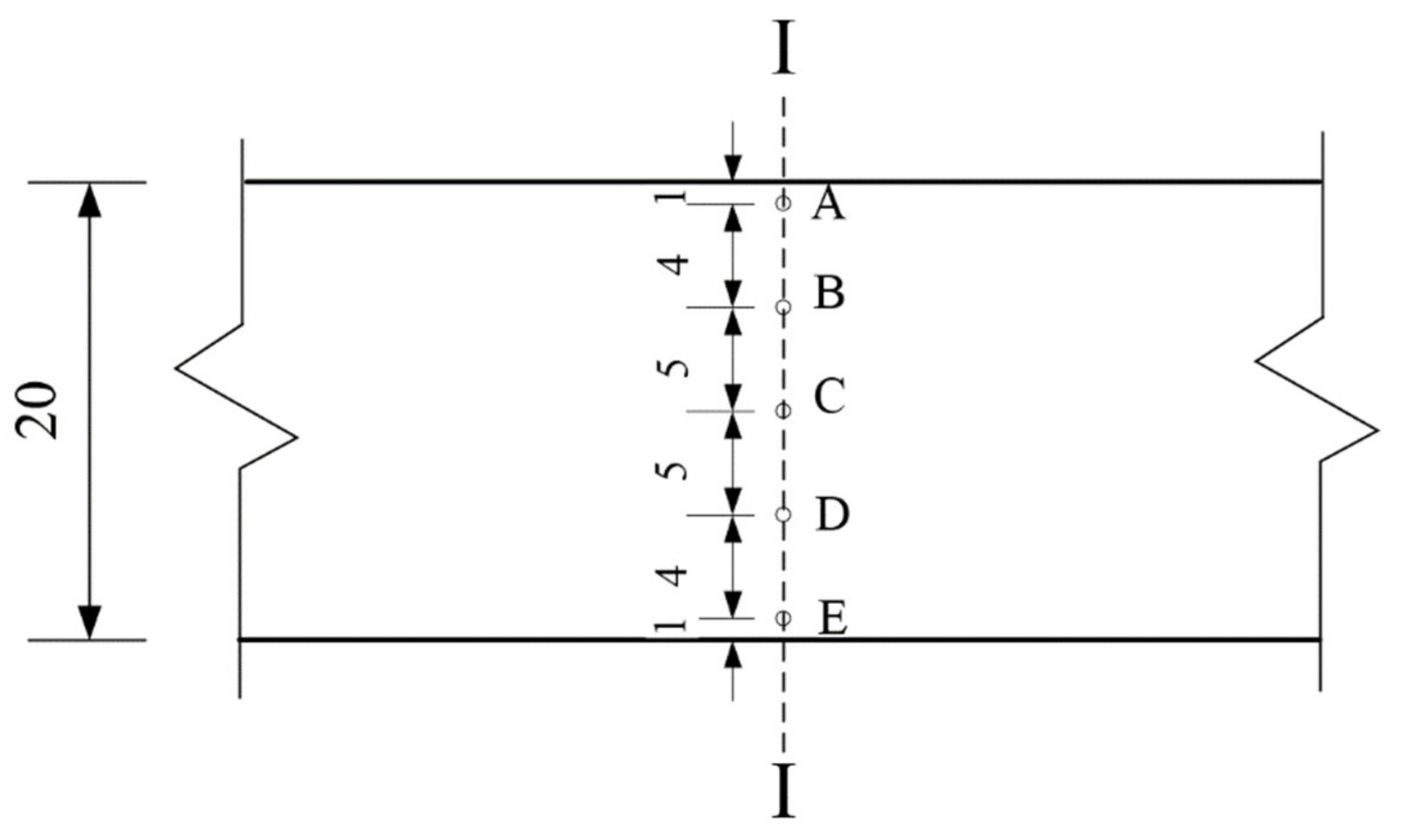
2.1. Establishment of the Model

In order to guide the later model test better, the beam model shown in Figure 1 was used for numerical simulation. This paper only considers the wind direction perpendicular to the cross beam of bridge tower and explores the general law of ice accretions. The direction of strong wind in the atmospheric boundary layer is mainly horizontal, but the wind attack angle may change slightly in the range of −3° to +3° [26]. The wind attack angle may increase when the wind speed decreases. Therefore, we set the flow field to the shape shown in Figure 2 to amplify the effect of wind attack angle on the icing process. The flow filed is divided by tetrahedral mesh and considering the cross beam is generally in the Ekman layer of atmospheric boundary layer where the atmospheric flow is basically a simple turbulent flow without considering compressibility. Therefore, the Realizable $k-\epsilon$ turbulence model suitable for boundary layer flow is selected for flow field calculation. The calculated results of all flow fields in this paper are convergent. The obtained wind attack angle in this model is about 26.6°, and the direction of it is oblique upward along the positive direction of X axis. In order to facilitate the identification of boundary in the flow field calculation, each wall of the flow field is divided into four groups: A, B, C, and D. The wall of group A is named inlet, which is used as the velocity inlet in the flow field calculation. The wall of group B is named airwall, which is the boundary of air region. The wall represented by C is named outlet as the outlet of air fluid for flow field calculation. The wall that D represents is named solidwall as the solid boundary of the beam in the flow field calculation. The gravity in the flow field calculation is set to 9.8 m/s² along the negative direction of Y axis.

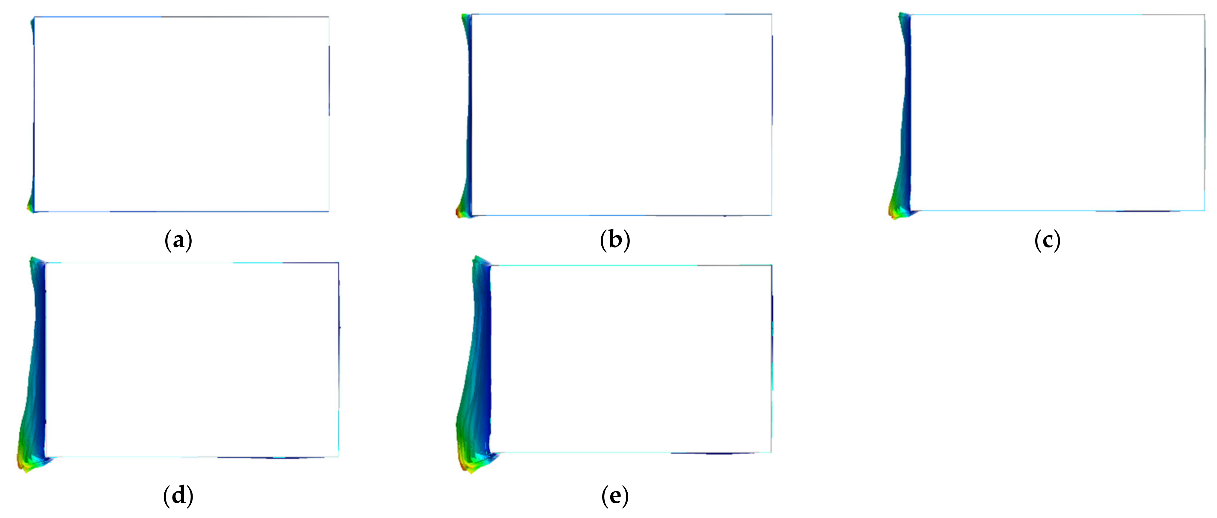
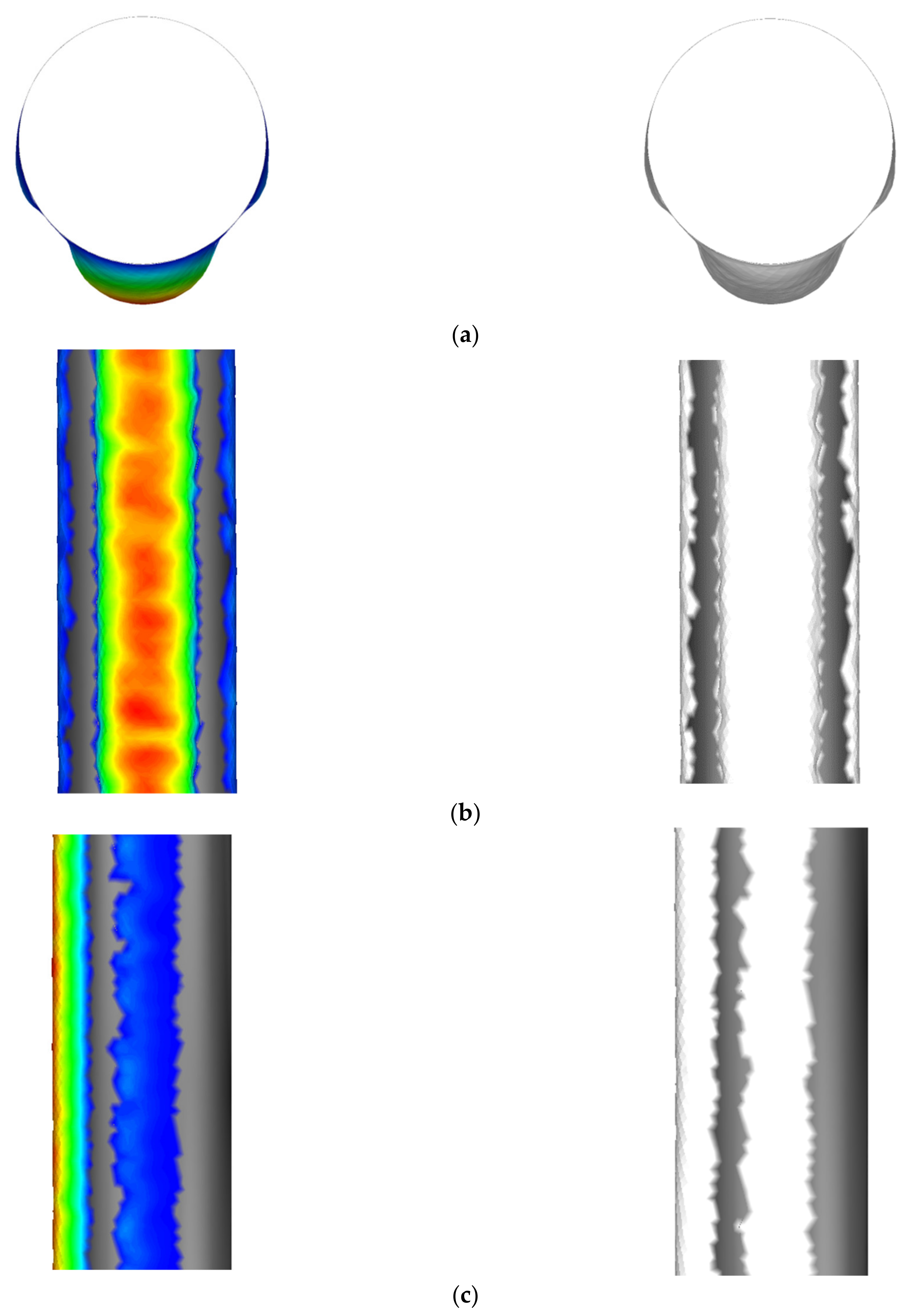
2.2. Effects of Wind

When calculating the flow field, it is necessary to set the velocity of the wind entering the flow field at inlet. Firstly, the effect of wind attack angle on the icing simulation results of cross beam was studied under wind speed of 10 m/s and temperature of −10 °C. The ice distributions of the cross beam under the wind attack angle of ±26.6° is shown in Figure 3.

Different wind speeds will lead to different results of flow field calculation that will result in different ice distributions on cross beam. In order to study the influence of different wind speeds on the icing simulation and to facilitate the guidance of the later model experiment, five wind-speed conditions for flow field calculation were set: 5 m/s, 10 m/s, 15 m/s, 20 m/s, and 25 m/s. The ambient temperature was set to −10 °C, the freezing time was set to 3600 s, and the side view of ice distribution of beam under different wind speeds is shown in Figure 4. The total mass of ice on cross beam at various wind speeds is shown in

Table 1. Total mass of ice on cross beam surface at different wind speeds.

Wind Speed (m/s)	Total Mass of Ice (kg)
5	0.2405
10	0.7054
15	1.334
20	2.275
25	3.55

.

Figure 3 shows that ice mainly attached to the windward surface of cross beam, and the distribution of ice on cross beam will influenced by wind attack angle. When the value of wind attack angle is positive, the ice on the bottom of windward surface will thicker than the ice on the top of windward surface, and negative wind attack angle will make the ice on the top windward surface thicker than the ice on the bottom of windward surface. According to Figure 4, the thickness of ice under the same conditions will increase continuously with the increase of wind speed; additionally, the difference of ice distribution on cross beam is more obvious. Shown as Figure 5, on the intersection line between section I-I and windward surface of cross beam, five reference points, marked A, B, C, D, and E, were selected to study the variations of ice thicknesses at different wind speeds. The ice thicknesses of the five reference points at different wind speeds were obtained by numerical simulation, and the curve graph of ice thicknesses of five points under different wind speeds was plotted.

It can be seen from Figure 6 that the ice thickness of point E is always the biggest in five reference points and also the thickness growth rate. It indicates that the position near the bottom edge of the windward surface is the main icing position. When wind speed is below 10 m/s, the ice thickness of point A is only second to point E, but the thickness growth rate is gradually slower than point D with the increase of wind speed. After the wind speed exceeds 15 m/s, the ice thickness of point D gradually exceeds point A, and the difference of ice thickness between two points expands constantly with the increase of wind speed. The reason for the change of the thickness of point A and point D is that with the increase of wind speed, the ice thickness on the bottom of windward surface increases faster than the other areas on the windward surface. It makes the main icing position no longer limited to the bottom of windward surface but gradually expands to the whole lower part of windward surface, which speeds up the ice thickness growth rate of point D. When wind speed is below 20 m/s, there is little change in the ice thickness of points B and C, and the ice thickness of points B and C is almost the same. It indicates that the position of points B and C are not easy to ice. When wind speed exceeds 20 m/s, the ice thickness increase trend of point B is not changed, but the thickness growth rate of point C begins to increase, and the difference of thickness between points B and C increases sharply. It can be seen from Figure 4 that this is also due to the extension of the main icing position on the lower part of windward surface.

As shown in Figure 7, the increase curve of total ice mass to wind speeds is drawn based on Table 1 when other conditions are same. Figure 7 indicates that the total ice mass and wind speed are positively correlated quadratic functions; the fitting equation based on the increased curve of total ice mass to wind speeds is as follows:

$$Y=0.00552V^2-0.00188V+0.1307$$

(1)

where Y is the total ice mass on cross beam, and V is the wind speed in flow fluid. The goodness-of-fit (R2) of the fitting equation and curve is 0.9998 meet the demand that R2 > 0.99. Therefore, the rule of the original curve can be analyzed by Formula (1).

According to the results of the numerical simulation about influence of different wind speeds to icing on cross beam, water freezes mainly on the windward surface of cross beam. The ice thickness on the windward surface increases constantly with the increase of wind speed. Although there are changes of ice distribution, the total ice mass and wind speed are positively correlated quadratic functions. When wind speed is below 10 m/s, the top edge and bottom edge of windward surface are the main icing position. When wind speed exceeds 15 m/s, the main icing position on the bottom of the windward surface will gradually extend to the whole lower part of windward surface.

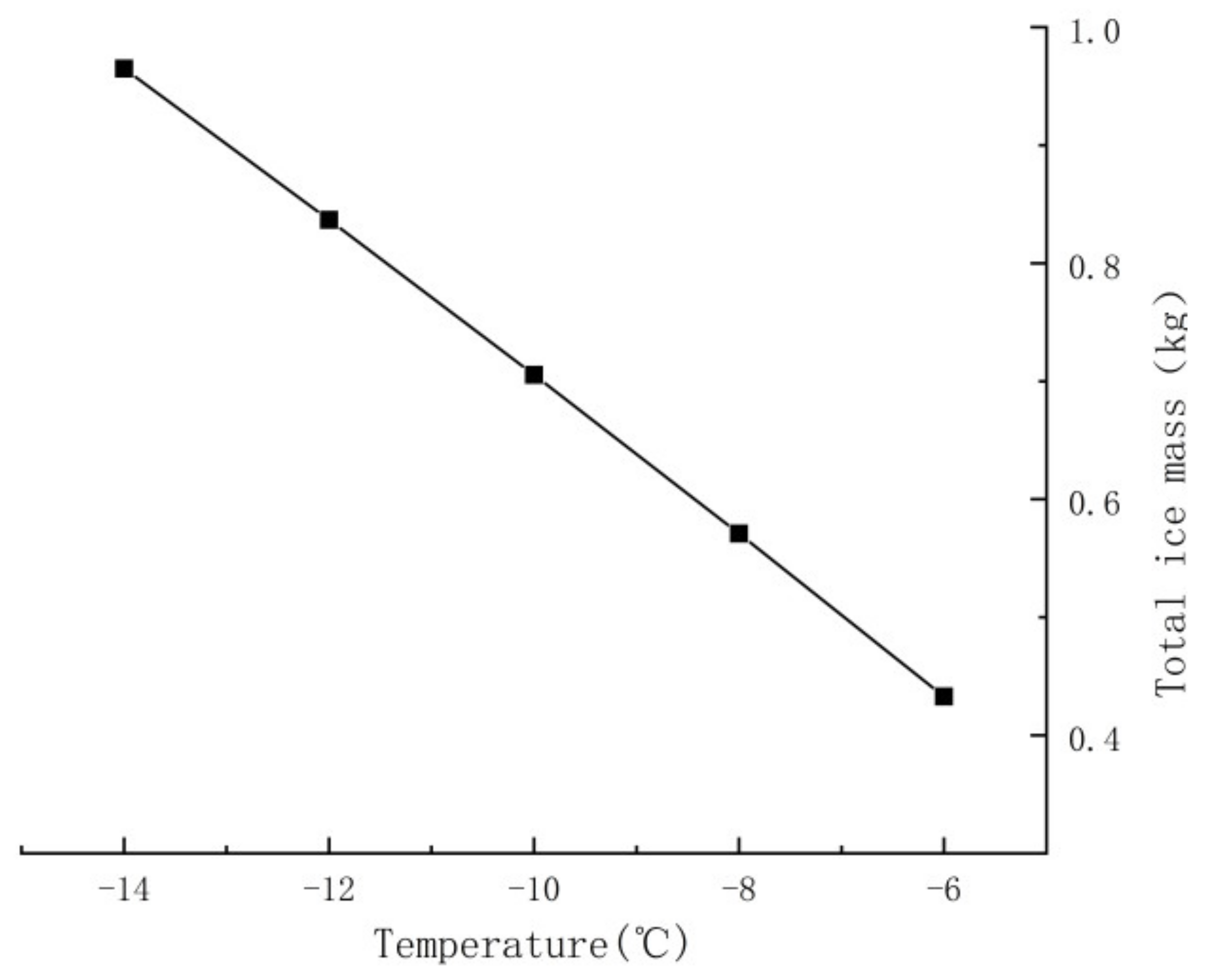
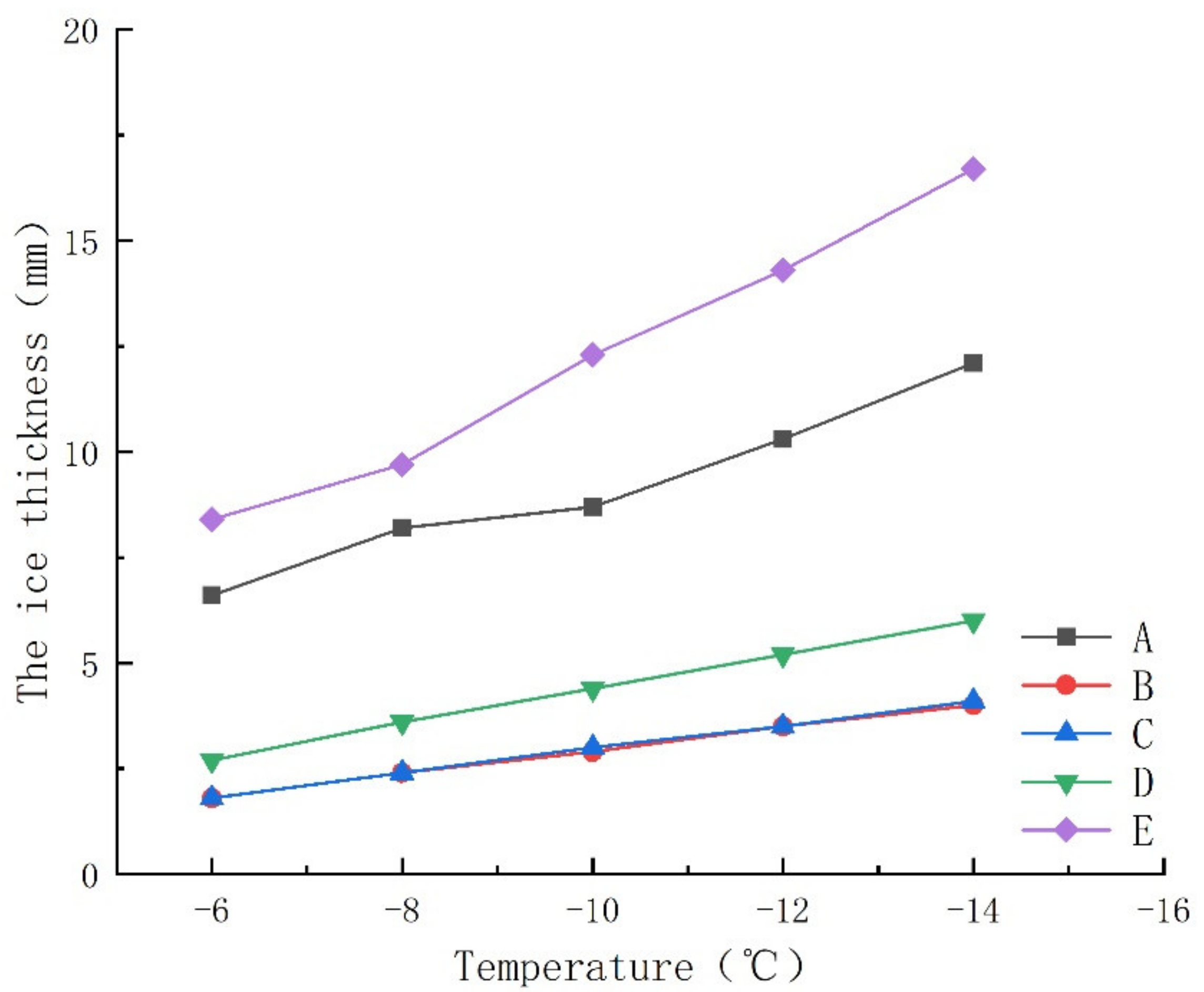
2.3. Effects of Ambient Temperature

Ambient temperature is an important factor affecting icing on the cross beam of bridge towers. In order to study the affecting of temperature to icing on the cross beam, this paper carried out an icing simulation experiment of the cross beam at five temperature conditions: −6 °C, −8 °C, −10 °C, −12 °C, and −14 °C. The wind speed was set to 10 m/s, and the freezing time was set to 3600 s. The side view of ice distribution of the cross beam under different temperatures is shown in Figure 8, and the total mass of ice on the cross beam at different temperature is shown in

Table 2. Total mass of ice on cross beam surface at different temperature.

Temperature (°C)	Total Mass of Ice (kg)
−6	0.433
−8	0.5709
−10	0.7054
−12	0.8367
−14	0.965

. In Figure 9, the curve graph of ice thicknesses of the five reference points under different temperatures is plotted.

It can be seen from Figure 9 that the ice thickness of each point increases constantly with the decrease in temperature. The thickness increase speed of each point is almost the same, so the thickness curve of each point shows a parallel trend. It indicates that the rule of ice distribution on windward surface is almost same at different temperatures. The curves of points E and A in Figure 9 show that the top edge and bottom edge of the windward surface are still the main icing position. The curves of points B, C, and D in Figure 9 show that with the temperature decrease, the main position of icing slightly expands. The main ice coverage positions are essentially constant, and the ice thickness changes little with the temperature decrease, which makes the ice thickness on the positions of points B, C, and D relatively thin. The maximum ice thickness of points B, C, and D is about 5 mm.

As shown in Figure 10, the increase curve of total ice mass to temperature is drawn based on Table 2 when other conditions are same. Figure 10 indicates that the total ice mass and temperature have a negatively linear relationship; the fitting equation based on the increase curve of total ice mass to temperature is as follows:

$$Y=-0.06649T+0.0373$$

(2)

where Y is total ice mass, and T is ambient temperature. The goodness-of-fit (R2) of the fitting equation and curve is 0.9998, meeting the demand that R2 > 0.99. Therefore, the rule of the original curve can be analyzed by Formula (2).

According to the Formula (1) and Formula (2), when the wind speed is 6.02 m/s, the absolute value of slopes of the two equations are equal. It indicates that within the given range of wind speed and temperature, the effects of temperature on icing are greater than that of wind when the wind speed is less than 6.02 m/s, and when the wind speed exceeds 6.02 m/s, the effects of wind will be greater than those of temperature.

Based on the results of the numerical simulation regarding influence of different temperatures to icing on the cross beam, the total ice mass and temperature display a negatively linear relationship. With the decrease of ambient temperature, the total ice mass on the cross beam increases constantly, and the ice thickness of each point shows a trend of uniform increase.

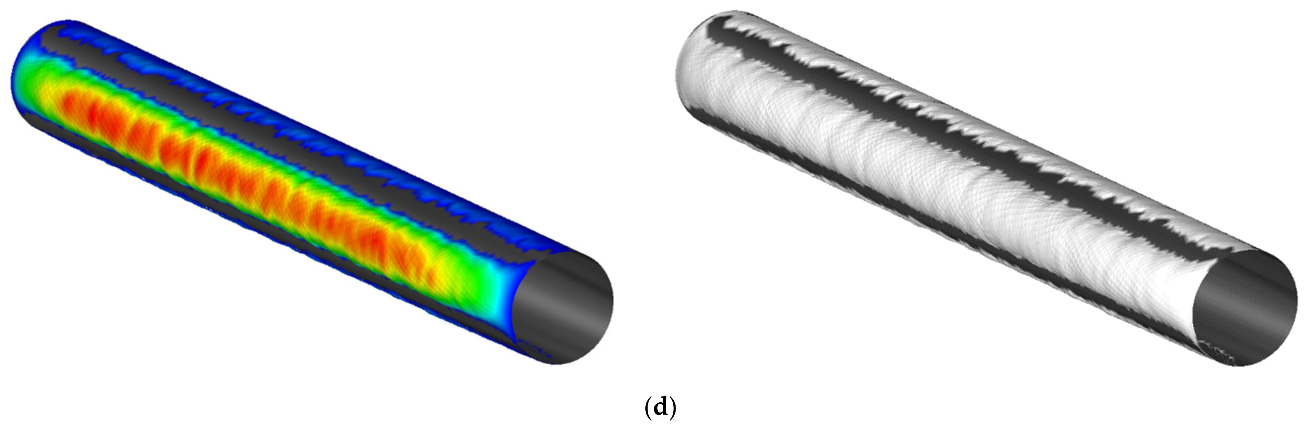
2.4. Validation of Numerical Simulation Method

According to the laboratory ice accretion test results of bridge cables obtained by Demartino et al. [22], a same-size bridge cable model (the nominal diameter is 160 mm and the length is 1.42 m) was established in ANSYS to validate the serviceability of the numerical simulation method. The wind speed was set to 17 m/s, the temperature was set to −5 °C, and the time was set to 1 h. The ice distribution of the simulation test of bridge cables is shown in Figure 11.

2.5. Verification of Mesh Independence and Time Steps Independence

When verifying the mesh independence, the mesh size of flow field were set to 0.25 m, 0.5 m, and 0.75 m, respectively. The wind speed was set to 10 m/s, and temperature was set to −10 °C. The ice accretion results of mesh independence were shown in Figure 12. When verifying the time steps independence, the time steps of the water droplet trajectory calculation were set to 120 s, 240 s, and 480 s, respectively. The wind speed was set to 10 m/s, and temperature was set to −10 °C. The ice accretion results of time steps independence were shown in Figure 13.

Figure 12 and Figure 13 show that the changes of mesh size and time steps have almost no effects on the ice distribution, which means the numerical simulation method has good mesh independence and time steps independence.

3. Study of Ice-Melting Measure

According to the results of icing simulation, this paper proposes a scheme of ice melting based on electric heating method. As shown in Figure 14, a kind of heating module that can be attached to a cross beam was designed. Because the carbon-fiber heating line has the characteristics of rapid heating-up, high electrothermal efficiency, and temperature stabilization [27], the heating module uses it as heat source. The heat will transfer to the ice and the beam to melt ice when the heat source generates heat.

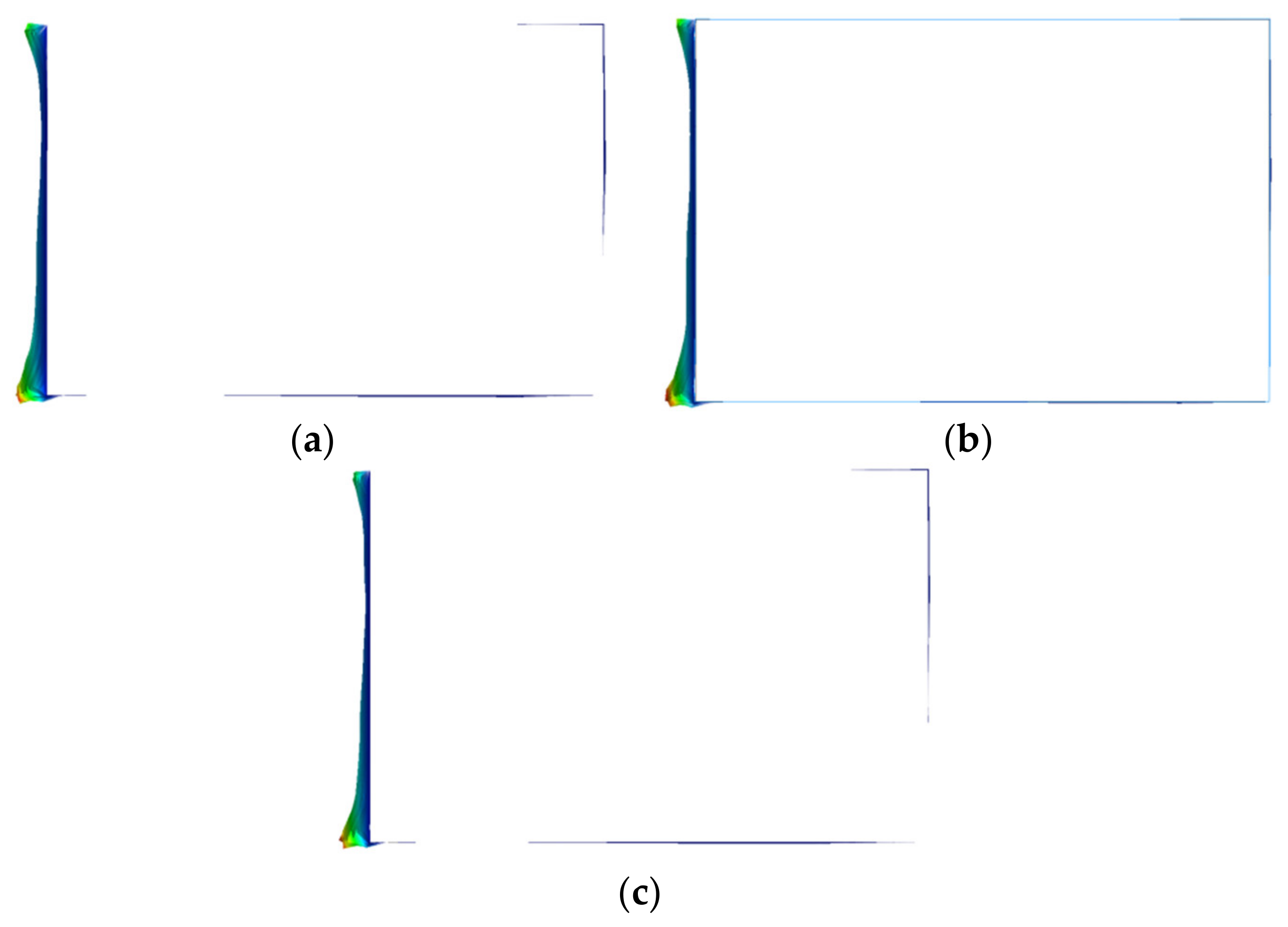
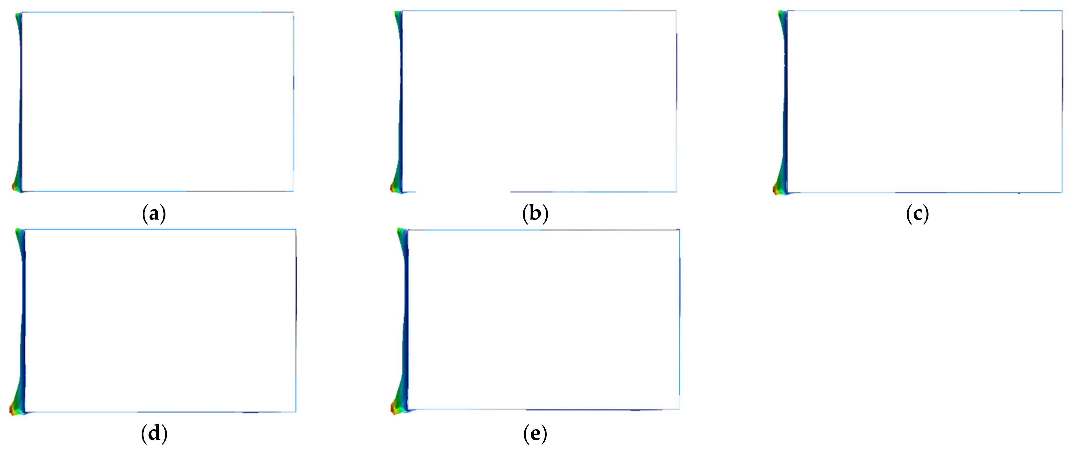
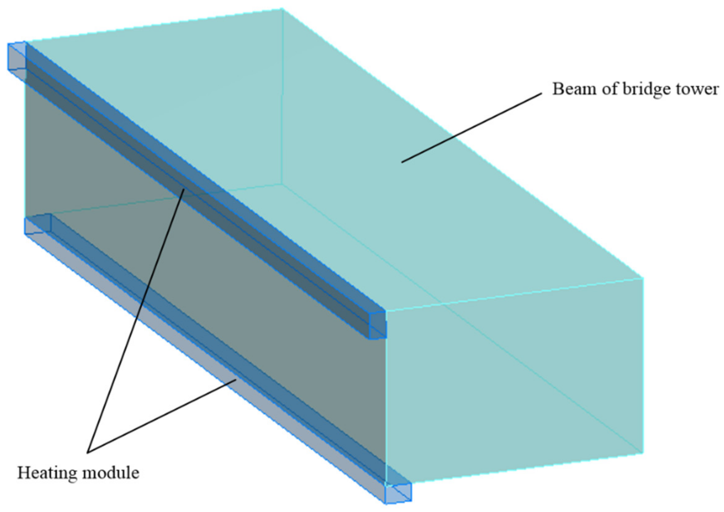
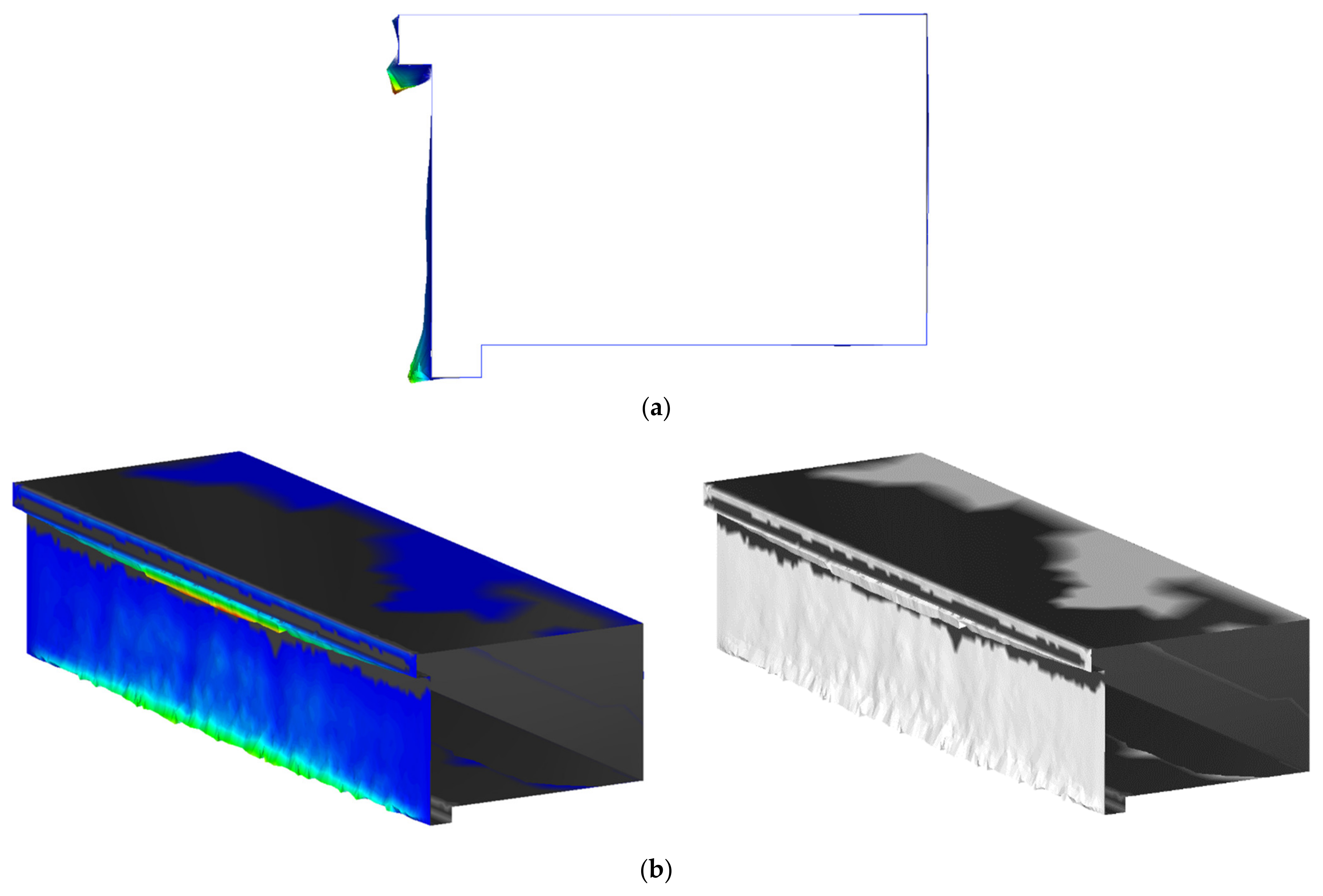
3.1. Effects of Heating Module Layout Position on Ice Simulation

Icing simulation of the cross beam shows that water freezes mainly on the windward surface, making the ice near the bottom and top edge of windward surface thicker than in other areas. At the same time, when the heating module works, a large amount of melted water that comes from melting ice and snow will flow along the beam surface under gravity. The melting water may freeze again outside the scope of the heating module and even form ice cones and icicles, which will cause greater security risks to traffic. Considering these problems, as shown in Figure 15, the heating modules are set on the positions of the largest ice thickness. This arrangement mode can melt as much ice on the windward surface as possible. The heating module on the bottom of the cross beam can prevent the melting water flowing to the bottom of the cross beam and freezing again.

To investigate the influence of heating modules to icing on the cross beam, a cross beam model with heating modules as shown in Figure 15 was established, where the t of heating module is 0.02 m, the w is 0.03 m, and the l is 1 m. The icing simulation was carried with this model. The wind speed was set to 10 m/s, the ambient temperature was set to −10 °C, and the freezing time was set to 3600 s. The ice distribution of the beam he with heating model is shown in Figure 16. The comparison between Figure 8c and Figure 16 shows that the heating modules bring a big change to the distribution of ice. The main icing area on the top of the windward surface moves to the bottom face of the top heating module, and the main icing area on the bottom of windward surface moves to the side face of the bottom heating module, which make the surface of heating module become the main area that ice attaches. This is good for the heating module because the module melts ice and snow by heating its surface, and the changes improve utilization efficiency of heat produced by the carbon-fiber heating line.

According to the results of the icing simulation, the model demonstrates efficient for melting ice and snow by setting heating modules on the cross beam. In addition, the changes of ice distribution make the heating module heat the ice and snow directly, which improves the efficiency of ice and snow melting and the energy utilization.

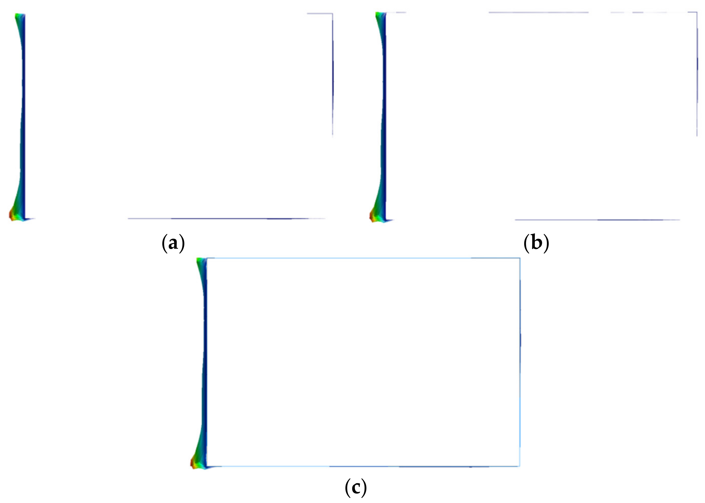
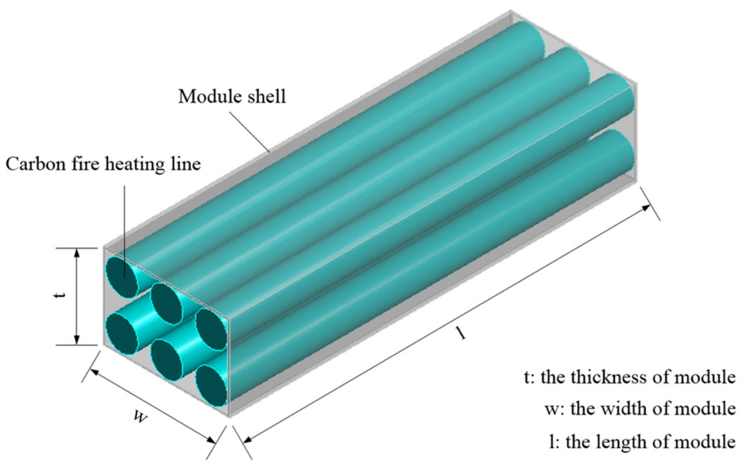
3.2. Effects of Geometrical Dimension of Heating Module on Icing Simulation

To study the effects of geometrical dimensions of the heating module on the icing simulation and explore more reasonable dimensions of the heating module to improve the melting efficiency, four groups of heating modules with different width and thickness were set: (a) w is 0.02 m, t is 0.01 m; (b) w is 0.02 m, t is 0.02 m; (c) w is 0.03 m, t is 0.03 m; and (d) w is 0.04 m, t is 0.03 m. The wind speed was set to 10 m/s, the temperature was set to −10 °C, the freezing time was set to 3600 s, and the ice distribution of each group on the cross beam is shown in Figure 17.

As shown in Figure 17, reducing the thickness of heating module on the top of windward surface will increase the ice thickness on module surface and make the ice distribution uneven, which makes the heating module unable to melt most of the ice in time. When the heating module works, it is easy for the large mass of ice to fall off, which brings great threat to road traffic safety. Thus, the heating module on the top of the windward surface needs to have a greater thickness to decrease the ice thickness on module surface and make the ice distribution more uniform. This is necessary for the module to melt most of the ice in time. The comparison of ice distribution on the top module between Figure 17c,d shows that under the same thickness of heating module, the larger width of module can reduce the thickness of ice on the bottom face of the module. This is helpful to melt ice completely. Increasing the thickness of the module also can enlarge the influence scope of the module, which will help to reduce ice on other areas. Therefore, when choosing the geometrical dimension of the heating module on the top of the windward surface, a larger width and thickness should be rationally selected on the results of icing simulation. Increasing the thickness of the heating module on the bottom of the windward surface can cause the ice to mainly freeze on the side face of the module. This is also helpful to melt ice. According to the results of icing simulation, the bottom of the cross beam does not ice easily. Additionally, the comparison between Figure 16a and Figure 17b shows that the width of the bottom module has little effect on ice distribution. Thus, the width of the bottom module can be advisably decreased to reduce heat loss and improve the energy-utilization efficiency.

The analyses of the icing simulations show that the width and the thickness of the top module can be increased rationally to reduce the ice thickness and make the ice distribute evenly, which is beneficial for the module to work. Increasing the thickness and decreasing the width of the bottom module rationally can make ice mainly form on the side face of module and reduce the heat loss.

4. Conclusions

This paper takes a scale model of the cross beam as an example and presents a new numerical simulation method to study the ice distributions on surface of the cross beam. This method can be used to study the influences of different factors to icing simulation and analyze the general rule of ice distribution characteristics on the surface of structures. Based on the results of the icing simulation, the scheme of ice melting was put forward, and we studied the feasibility and validity of the scheme.

The main conclusions of the present are as follows:

(1)

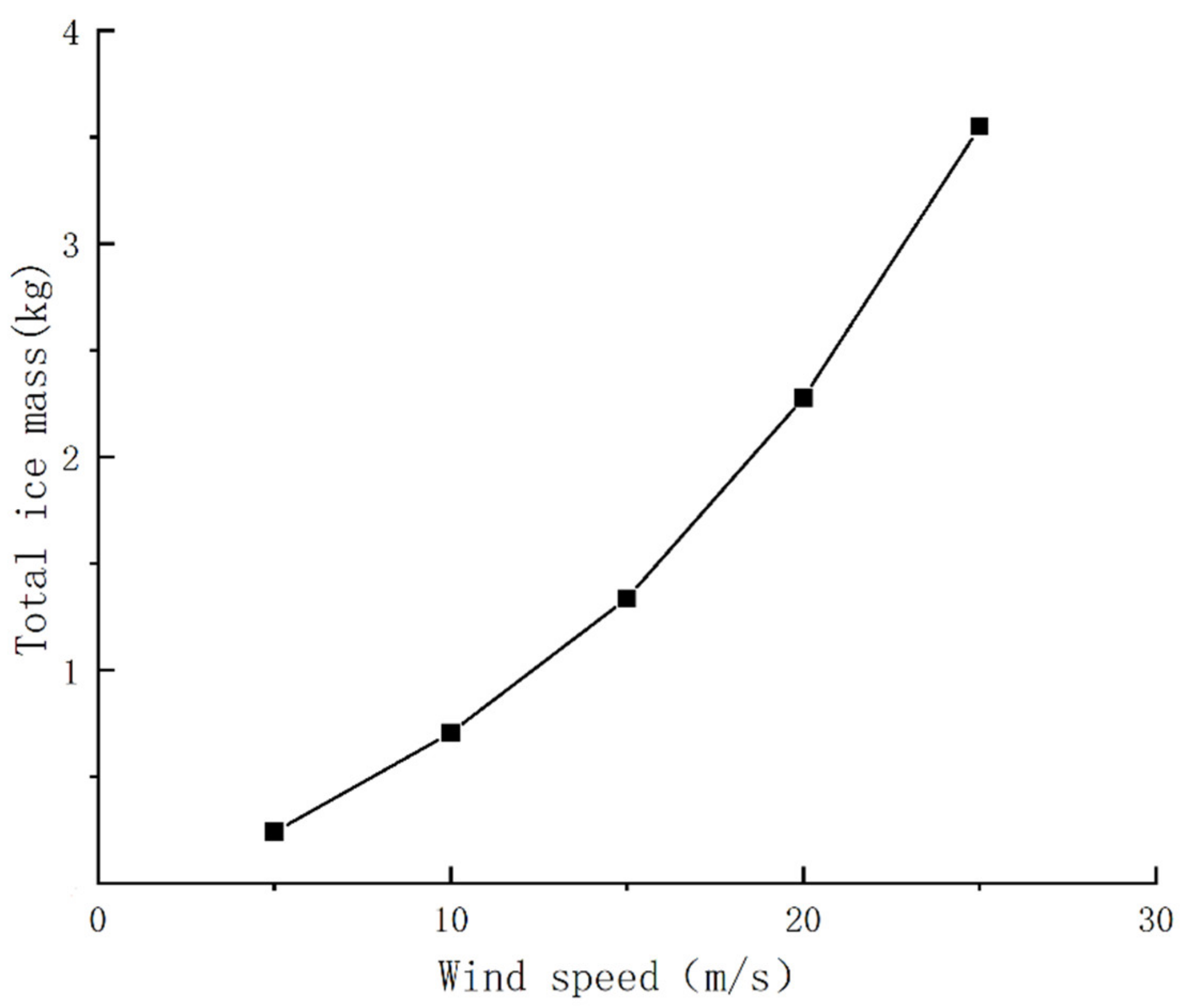
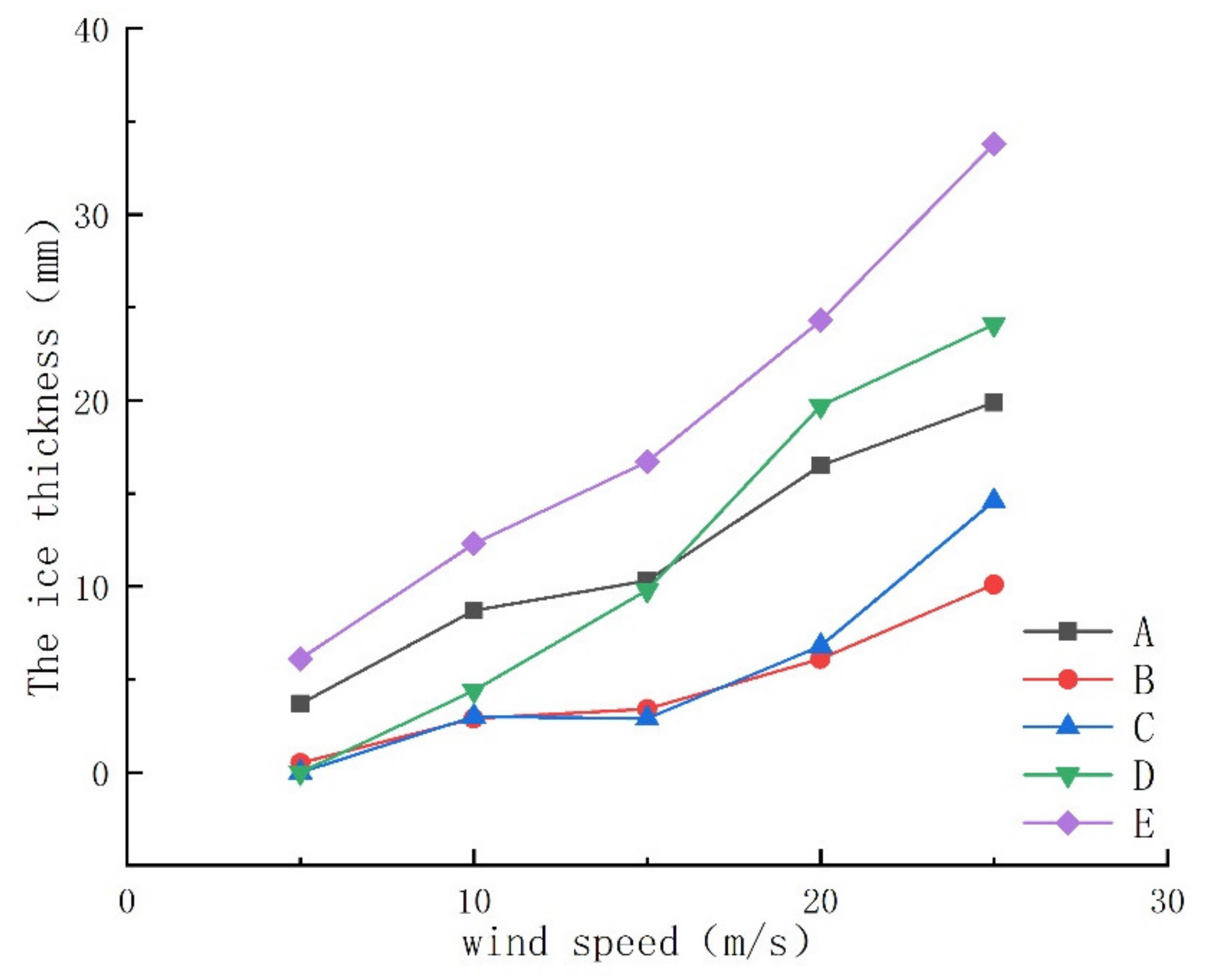
In the ice accretions simulation of the cross beam of a bridge tower, the total ice mass and wind speed are positively correlated quadratic functions. The total ice mass and temperature show a negatively linear relationship. In addition, the influence of wind on the icing process is greater than temperature within the given range of wind speed and temperature.

(2)

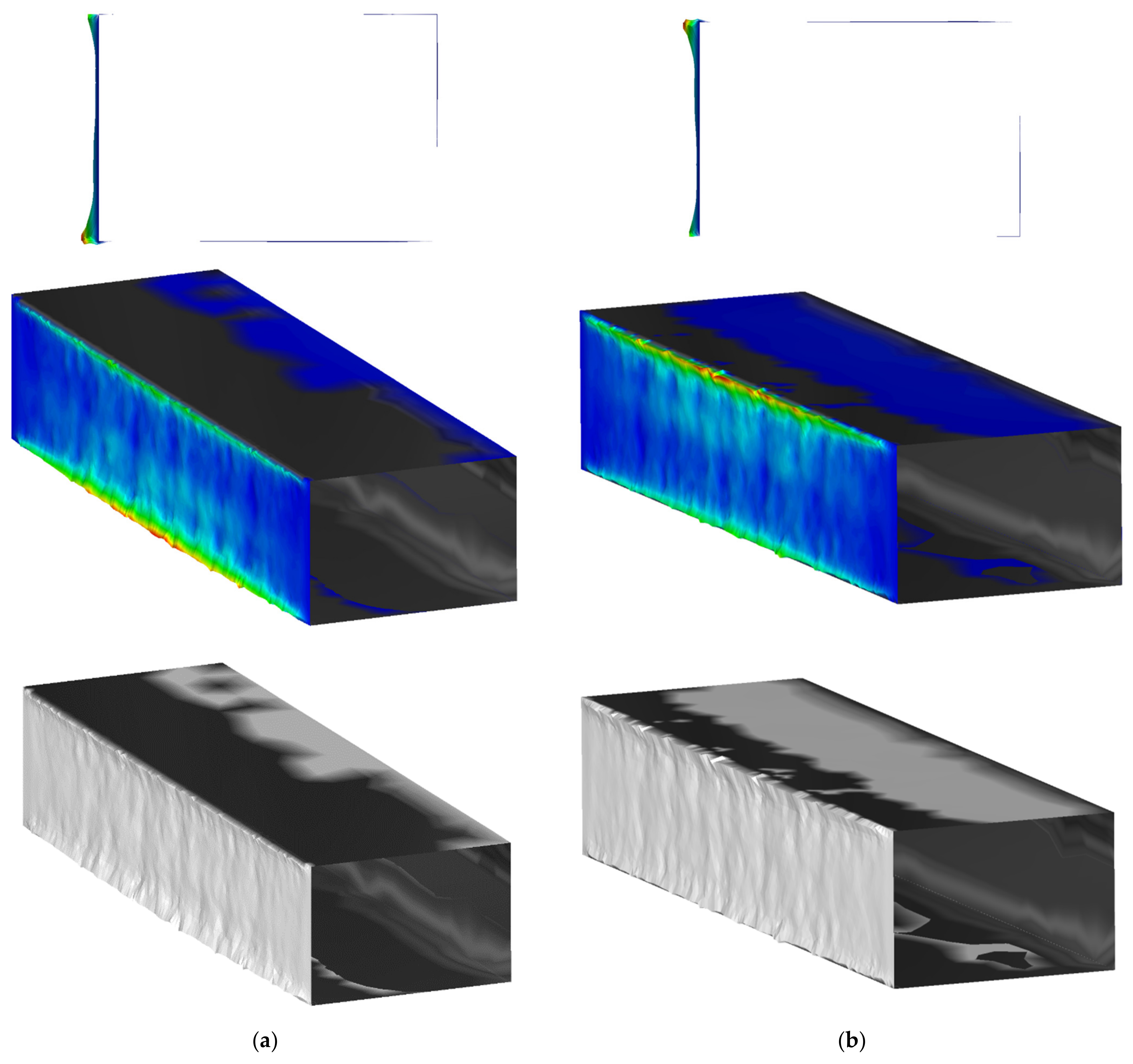
When the wind attack angle is positive, the ice near the bottom edge of the windward surface will be thicker than top edge, and the bottom ice thickness increases faster than top ice with the increase of wind speed, and negative wind attack angle is the opposite.

(3)

After the modules were set, the changes of ice distribution show that using heating modules to melt ice is reasonable and effective. To prevent the melted water from flowing to the bottom surface of the cross beam and freezing again, a heating module should be arranged on the bottom surface. Adjusting the geometrical dimension of the heating module reasonably can reduce heat loss, improve the efficiency of ice melting, and save energy.

(4)

This ice accretion numerical simulation method has good serviceability, and the results of the method conform to reality. Additionally, the method has good mesh independence and time steps independence.

(5)

The size and the location of the actual cross beam are not convenient to study ice-melting schemes through field tests. Therefore, when designing the ice-melting scheme of an actual cross beam, the numerical simulation method proposed in this paper can be used to study the size and layout position of a heating module that is suitable for the actual cross beam.

References

1. Cao, S.; Jalali, H.H.; Dragomirescu, E. Wind-induced response of inclined and yawed ice-accreted stay cable models. Shock. Vib. 2018, 2018, 6853047. [Google Scholar] [CrossRef]
2. Andre, J.; Kiremidjian, A.; Georgakis, C.T. Statistical mdeling of time series for ice accretion detection on bridge cables. J. Cold Reg. Eng. 2018, 32, 04018004. [Google Scholar] [CrossRef]
3. Lyu, W.; Pu, H.; Chen, J.N.; Gao, Z. Numerical study on optimal scheme of the geothermally heated bridge deck system. Energies 2020, 13, 6633. [Google Scholar] [CrossRef]
4. Ozsoy, A.; Yildirim, R. Prevention of icing with ground source heat pipe: A theoretical analysis for Turkey’s climatic conditions. Cold Reg. Sci. Technol. 2016, 125, 65–71. [Google Scholar] [CrossRef]
5. Yiqiu, T.; Chi, Z.; Huijie, L.; Hao, S.; Huining, X. Experimental and numerical analysis of the critical heating strategy for hydronic heated snow melting airfield runway. Appl. Therm. Eng. 2020, 178, 115508. [Google Scholar] [CrossRef]
6. Lei, G.; Yu, X.B.; Li, T.; Habibzadeh-Bigdarvish, O.; Wang, X.; Mrinal, M.; Luo, C. Feasibility study of a new attached multi-loop CO2 heat pipe for bridge deck de-icing using geothermal energy. J. Clean. Prod. 2020, 275, 123160. [Google Scholar] [CrossRef]
7. Mirzanamadi, R.; Hagentoft, C.E.; Johansson, P. An analysis of hydronic heating pavement to optimize the required energy for anti-icing. Appl. Therm. Eng. 2018, 144, 278–290. [Google Scholar] [CrossRef]
8. Yu, X.; Hurley, M.T.; Li, T.; Lei, G.; Pedarla, A.; Puppala, A.J. Experimental feasibility study of a new attached hydronic loop design for geothermal heating of bridge decks. Appl. Therm. Eng. 2019, 164, 114507. [Google Scholar] [CrossRef]
9. Habibzadeh-Bigdarvish, O.; Yu, X.B.; Li, T.; Lei, G.; Banerjee, A.; Puppala, A.J. A novel full-scale external geothermal heating system for bridge deck de-icing. Appl. Therm. Eng. 2020, 185, 116365. [Google Scholar] [CrossRef]
10. Tuan, C.Y. Roca Spur Bridge: The implementation of an innovative deicing technology. J. Cold Reg. Eng. 2008, 22, 6853047. [Google Scholar] [CrossRef]
11. Dehghanpour, H.; Yilmaz, K. Heat behavior of electrically conductive concretes with and without rebar reinforcement. J. Mater. Sci. 2020, 26, 471–476. [Google Scholar] [CrossRef]
12. Sassani, A.; Arabzadeh, A.; Ceylan, H.; Kim, S.; Sadati, S.S.M.; Gopalakrishnan, K.; Taylor, P.C.; Abdualla, H. Carbon fiber-based electrically conductive concrete for salt-free deicing of pavements. J. Clean. Prod. 2018, 203, 799–809. [Google Scholar] [CrossRef]
13. Xie, X.M.; Su, J.F.; Guo, Y.D.; Wang, L.Q. Evaluation of a cleaner de-icing production of bituminous material blending with graphene by electrothermal energy conversion. J. Clean. Prod. 2020, 274, 122947. [Google Scholar] [CrossRef]
14. Lai, J.X.; Liu, C.; Gong, C.B. Research situation and prospect for highway snowmelt deicing technology with electric heat tracing. Appl. Mech. Mater. 2011, 71–78. [Google Scholar] [CrossRef]
15. Mohammed, A.G.; Ozgur, G.; Sevkat, E. Electrical resistance heating for deicing and snow melting applications: Experimental study. Cold Reg. Sci. Technol. 2019, 160, 128–138. [Google Scholar] [CrossRef]
16. Liu, X.; Rees, S.J.; Spitler, J.D. Modeling snow melting on heated pavement surfaces. Part I: Model development. Appl. Therm. Eng. 2007, 27, 1115–1124. [Google Scholar] [CrossRef]
17. Kim, H.S.; Ban, H.; Park, W.J. Deicing concrete pavements and roads with Carbon Nanotubes (CNTs) as heating elements. Materials 2020, 13, 2504. [Google Scholar] [CrossRef]
18. Liu, K.; Huang, S.; Xie, H.; Wang, F. Multi-objective optimization of the design and operation for snow-melting pavement with electric heating pipes. Appl. Therm. Eng. 2017, 122, 359–367. [Google Scholar] [CrossRef]
19. Lai, Y.; Liu, Y.; Ma, D.X.; Wang, P.; Su, X. The influence of wind speed on melting ice on concrete pavement with carbon fiber heating wire. Int. Workshop Mater. Chem. Eng. 2018, 2018, 313–318. [Google Scholar]
20. Wu, J.; Yang, F.; Liu, J. Research on carbon fiber heating wire for pavement deicing. J. Test. Eval. 2015, 43, 574–581. [Google Scholar] [CrossRef]
21. Ypa, B.; Rv, B.; Yang, L.B.; Xhac, D. An experimental study on dynamic ice accretion and its effects on the aerodynamic characteristics of stay cables with and without helical fillets. J. Wind Eng. Ind. Aerodyn. 2020, 205, 104326. [Google Scholar] [CrossRef]
22. Demartino, C.; Koss, H.H.; Georgakis, C.T.; Ricciardelli, F. Effects of ice accretion on the aerodynamics of bridge cables. J. Wind Eng. Ind. Aerodyn. 2015, 138, 98–119. [Google Scholar] [CrossRef]
23. Guo, P.; Li, S.; Wang, D. Effects of aerodynamic interference on the iced straddling hangers of suspension bridges by wind tunnel tests. J. Wind Eng. Ind. Aerodyn. 2019, 184, 162–173. [Google Scholar] [CrossRef]
24. Xu, F.Y.; Yu, H.Y. Effect of ice accretion on the aerodynamic responses of a pipeline suspension bridge. J. Bridge Eng. 2020, 25, 04020091. [Google Scholar] [CrossRef]
25. Zhang, M.J.; Xu, F.Y.; Han, Y. Assessment of wind-induced nonlinear post-critical performance of bridge decks. J. Wind Eng. Ind. Aerodyn. 2020, 203, 104251. [Google Scholar] [CrossRef]
26. Zhang, X.; Sun, X.F.; Zhou, W.S.; Zhang, Y.X. Monitoring of stay-cable icing based on electro-mechanical impedance and principal component analysis. J. Harbin Eng. Univ. 2020. [Google Scholar] [CrossRef]
27. Zhao, H.; Dai, J.; Wu, K.; Kong, F. Experimental and modeling analysis of thermal characteristics in carbon fiber wires. Heat Trans. 2020, 49, 1863–1876. [Google Scholar] [CrossRef]
Figure 1. Beam model (cm).
Energies 14 05584 g001
Figure 2. Flow field model. (a) Mesh arrangement of flow field model. (b) Size of the flow field model and name of the boundaries (m).
Energies 14 05584 g002
Figure 3. The ice distributions of cross beam at different wind attack angles. (a) The wind attack angle is +26.6°. (b) The wind attack angle is −26.6°.
Energies 14 05584 g003
Figure 4. Side view of ice distribution of beams at different wind speeds. (a) The wind speed is 5 m/s. (b) The wind speed is 10 m/s. (c) The wind speed is 15 m/s. (d) The wind speed is 20 m/s. (e) The wind speed is 25 m/s.
Energies 14 05584 g004
Figure 5. Reference points position (cm).
Energies 14 05584 g005
Figure 6. The changes of ice thickness at different wind speeds.
Energies 14 05584 g006
Figure 7. The changes of total ice mass at different wind speeds.
Energies 14 05584 g007
Figure 8. The side view of ice distribution of beams at different temperature. (a) The temperature is −6 °C. (b) The temperature is −8 °C. (c) The temperature is −10 °C. (d) The temperature is −12 °C. (e) The temperature is −14 °C.
Energies 14 05584 g008
Figure 9. The changes of ice thickness at different temperatures.
Energies 14 05584 g009
Figure 10. The changes of total ice mass at different temperatures.
Energies 14 05584 g010
Figure 11. The bridge cable ice distributions of simulation test. (a) Cross-sectional view of cable ice distribution in simulation test. (b) Front view of cable ice distribution in simulation test. (c) Side view of cable ice distribution in simulation test. (d) The 3-D view of cable ice distribution in simulation test. The comparison between the simulation test result and the laboratory ice accretion test result that under the same conditions. Ref [22] shows that the result of the numerical simulation method conforms to reality.
Energies 14 05584 g011aEnergies 14 05584 g011b
Figure 12. The ice distributions at different mesh size. (a) The max mesh size is 0.25 m. (b) The max mesh size is 0.5 m. (c) The max mesh size is 0.75 m.
Energies 14 05584 g012
Figure 13. The ice distributions at different time steps. (a) The time steps are 120 s. (b) The time steps are 240 s. (c) The time steps are 480 s.
Energies 14 05584 g013
Figure 14. Heating module details.
Energies 14 05584 g014
Figure 15. Schematic diagram of heating module positions.
Energies 14 05584 g015
Figure 16. The ice distributions of cross beam. (a) Side view of ice distribution. (b) The 3-D view of ice distribution.
Energies 14 05584 g016
Figure 17. Side view of ice distribution on cross beam with different dimension of module. (a) The model width is 0.02 m and the thickness is 0.01 m. (b) The model width is 0.02 m and the thickness is 0.02 m. (c) The model width is 0.03 m and the thickness is 0.03 m. (d) The model width is 0.04 m and the thickness is 0.03 m.
Energies 14 05584 g017