Abstract
Energy system models for the analysis of future scenarios are mainly driven by the set of energy service demands that define the broad outlines of socio-economic development throughout the model time horizon. Here, the long-term effects of the COVID-19 pandemic on the drivers of the industrial production in six energy-intensive subsectors are addressed using Vector AutoRegressive models. The model results are computed either considering or not considering the effects of the pandemic. The comparison to established pre-pandemic trends allows for validating the robustness of the selected model. The anticipated effect of the pandemic to 2040 shows a long-term reduction by 3% to 10%, according to the different subsector, in the industrial energy service demand. When the computed service demands are used as input to the TIMES-Italy model, which shows good capability to reproduce the energy consumption of the industrial sectors in the period 2006–2020, the impact of the pandemic on energy consumption forecasts can be assessed in a business-as-usual scenario. The results show how the long-term effects of the shock caused by the pandemic could lead, by 2040, to a total industrial energy consumption 5% lower than what was foreseen before the pandemic, while the energy mix remains almost unchanged.
1. Introduction and Objectives
Energy system optimization models serve as a valuable tool to explore the uncertainty around the future evolution of an energy system over medium-to-long-term time scales and to assess the consequences of alternative policy strategies and the competitiveness of current and future energy technologies. Energy models encompassing the four dimensions of Energy, Economy, Engineering and Environment [1]—the so called “4Es”—such as those belonging to the TIMES framework [2], represent a widespread choice for the exploration of contrasted future scenarios. TIMES (an acronym for The Integrated MARKAL-EFOM System) is an economic model generator that provides a technology-rich basis for representing the energy dynamics of the evolution of a specific energy system [2], depicted through a so-called Reference Energy System (RES). The RES is a network diagram identifying all the technologies, commodities and commodity flows of the system under study, as well as the relationships among those entities over a multi-period time horizon. End-use energy service demands (e.g., for the industrial sector debated in this work, the projected production of steel, aluminum, zinc, copper, cement, ceramics, glass, high value chemicals, ammonia, methanol, chlorine and paper [3]) are used as input to the model. Based on them, the TIMES solution algorithm compute a least cost path for the energy system, by simultaneously finding the value of all the decision variables of the model (i.e., the installed capacity and activity level of each technology, as well as the quantity of commodities consumed and produced), based on the techno-economic characteristics of the technologies included in the model dataset, and considering a wide set of constraints, related typically to environmental objectives or the limited availability of some fuels [2].
Estimates of energy service demands are generally provided by the modeler, either through exogenously specified arrays of values obtained from accepted external sources [4], or by computing them by means of Equation (1), where D is a service demand, t the time step, δ the demand driver and e the elasticity of the demand to its driver [2].
Dt = Dt−1 × [1 + (δt/δt−1 – 1) × et−1].
In both options, the set of energy service demands should be internally coherent, with respect to both the different sectors of the energy system and the different regions represented in the model.
If energy service demands are computed through Equation (1), a twofold challenge arises. On one hand, when driver projections are retrieved from external sources, those drivers should be internally coherent as well. In the case of the JRC-EU TIMES Model [5] and the EUROfusion TIMES Model [6] (formerly the EFDA-TIMES Model [7]), the GEM-E3 general dynamic equilibrium model, which combines projections of population growth, energy prices, technical progress, energy intensity and labor productivity evolution, generating a series of national macroeconomic drivers [5], is used to accomplish that purpose [8]. On the other hand, elasticities should be computed based on econometric analyses and be able to capture changing patterns in energy service demands in relation to socio-economic growth, such as a saturation in some energy end-use demands, increased urbanization, or changes in consumption patterns once the basic needs are satisfied [2].
Addressing these challenges properly is complex. When general equilibrium macroeconomic models are used to generate sets of coherent drivers, the requested modeling effort for the drivers becomes comparable to the one carried out to develop the energy system model. Moreover, once the set of drivers is available, the quantitative literature on the elasticities of energy service demands to their drivers is very limited. (In the case of the industrial sector, addressed in this paper, elasticities are set equal to 1 for the entire time horizon, as the drivers already correspond to the service demands.) This paper aims at providing a methodology to overcome the above-mentioned challenges.
Looking at the historical global trends of the energy service demand for Europe and Italy, the five years between 2014 and 2019 saw a steady economic recovery from the last global crisis, started in 2008 [9], coupled with a rise in demand for energy commodities [10]. The unprecedented global crisis connected to the outbreak of the pandemic undermined that recovery, leading to a sudden, unexpected economic collapse [9]. The widespread adoption of total lockdown measures adopted since the first moments to contain the spreading of the disease had an immediate effect on energy use, among other aspects of daily life: total primary energy consumption dropped by about 10% in 2020 [9]. Even though, after a year, the industrial production is now close to its pre-pandemic level all around the world [11]—and that applies to Italy, too [12], where the fastest economic expansion since the 1970s is expected for 2021 after a deep recession [13]—all the economic sectors may observe long-term effects of a structural component in the energy demand drop, as identified for instance in [14] for the transport sector. Instead, no published work so far has shown that the same is happening in the industry sector: in this paper, we develop a mathematical model to predict long-lasting effects of the COVID-19 pandemic on that sector. The long-lasting effects of the pandemic on the whole economy are addressed in [15], where sectors other than transportation are analyzed, relating the overall reduction in the environmental pressure (CO2 emissions) in response to the recession to the energy component, due to the reduction in the consumption, which could also affect the long run with larger impacts than macroeconomic effects. Here, we assume that the drop in the energy consumption is, in the industrial sector, mainly related to the reduction in the manufacturing activity, as an effect of the degrowth of activities in other sectors (e.g., the contraction in buildings construction demand is directly reflected on cement production). Note, however, that the pandemic might also have pushed the different sectors towards the adoption of a different technology mix, which could result in less energy consumption.
During the last year, several works assessed the effects of the pandemic on energy consumption. The change in energy intensity and electricity demand during lockdowns, assessed on different spatial scales in [16], leads to different considerations for energy recovery in areas of the world with the more diverse behaviors, while [17] investigated the electricity demand fluctuation between two subsequent years (2019 and 2020) on a limited spatial scale and [18] the most recent Chinese oil and electricity demand trends in order to drive future policies in the framework of a sustainable recovery. As a common point, those and several other works all focus on final energy use, providing future insights via a simulation approach. Nonetheless, they neglect the underlying socio-economic driver perturbations that would inevitably influence the long-term energy service demand evolution. Attempts to model the response to the pandemic crisis in the evolution of economic indicators such as GDP have been made, as, for instance, in [19], but the results are generally short-term projections that do not fit the needs of long-term analyses performed by energy system optimization models. Furthermore, even considering the possibility of extrapolating long-term forecasts starting from such results, the lack of literature that analyzes more specific socio-economic drivers remains a problem.
In this paper, a simple and time-saving methodology to avoid dealing with complex general equilibrium models such as GEM-E3 is developed, based on the compact Vector AutoRegressive (VAR) model, to project the energy service demands of the most energy-intensive Italian industrial subsectors. The model reliability is verified against the projections used in the PRIMES model (the reference model used to assess the Italian Integrated National Energy and Climate Plan [20]), obtained in turn through a macroeconomic general equilibrium model [4]. After having successfully tested the VAR model to project industrial energy service demands just relying on the historical data up to 2019, the same model is then used to assess to what extent the recent COVID-19 pandemic can have structural effects on socio-economic drivers and energy use in Italy. The developed drivers are then used in an energy-economy optimization model tailored to the Italian RES, namely, the TIMES-Italy model. TIMES-Italy is a model instance of the TIMES family for the development of perspective energy scenarios for Italy [21]. It was developed and maintained at ENEA, the Italian National Agency for new technologies, energy and sustainable economic development, primarily for supporting national energy strategies. It describes the Italian energy system in its totality, from the extraction and import of primary energy to the satisfaction of the demands for energy services, in the transportation, buildings, industrial and agricultural sectors. It was used to produce the Italian National Energy Strategy (SEN) [22] on a time horizon extended until 2030. However, the tool is capable of performing long-term energy projections until 2050. Starting from 2006, the base year to which the model is calibrated (i.e., it matches the actual energy statistics provided by the national energy balances [23]), energy consumption and the related emissions of greenhouse gases, among other aspects, are computed by the model on the basis of the dataset of current and future energy technologies. By selecting the future optimal level of capacity and activity of each energy technology included in the model, each scenario depicts a least cost solution to satisfy the set of energy service demands, also taking into account user-defined constraints on the maximum exploitation of some resources or the short-term penetration of innovative technologies, as well as the policy constraints on the maximum amount of CO2 emissions over a certain time period. In this paper, in a business-as-usual scenario, the medium- and long-term projections of energy demand, resulting from the industrial sector driver evolution computed accounting for or neglecting the effect of the pandemic, are compared. The post-pandemic projections are finally used to investigate the anticipated structural effect of the pandemic on the Italian industrial energy consumption.
The paper is structured as follows. In Section 2, the development of the suitable Auto Regressive models to obtain the projections of industrial production is illustrated. In Section 3, the outcomes of the model are first validated against the pre-pandemic forecasts attached to the Italian Integrated National Energy and Climate Plan. Then, the results obtained accounting for the pandemic effects are presented and discussed, sector by sector. The outcomes of long-term industrial production projections are applied in Section 4 to the TIMES-Italy model, in order to quantify their impact on industrial energy consumption from the year 2020 to 2040. The conclusions of the work are presented in Section 5.
2. Model Development
Industrial production represents an important set of socio-economic drivers utilized to compute energy consumption projections for the entire industrial sector of a country. Six industrial subsectors are considered starting from the typical classification of the IEA Statistics (also embraced by the Italian National Statistics Institute ISTAT): iron and steel; Non-ferrous metals; Chemicals; Non-metallic minerals; Pulp and paper; and Other industrial sectors. The historical datasets considered here consist of monthly values of the Italian industrial production index of such sectors (base 2015 = 100) from January 1990 to April 2021 [24].
Accurate projections for the energy service demand for the industrial subsectors can be non-trivial to perform, given the restricted datasets at disposal and the scarce literature due to the specificity of such sectors and the limited geographical scale. The difficulty in the definition of explanatory and exogenous variables, i.e., the variables needed for such projections and their future values, adds to that, and could dangerously increase the overall arbitrariness of the results [25]. For the abovementioned reasons, VAR models turn out to be useful, considering that the benefits of modeling all the variables to forecast jointly rather than one equation at a time are well established [26], without the need of trying to necessarily define exogenous variables. In the same context of the COVID-19 pandemic, similar tools have already been used for the forecasting of infection cases and deaths from the virus [18].
VAR models are typically used to forecast multiple time-series variables in a single system of equations and to analyze the dynamic impact of the disturbance factors contained in the system variable. They were first proposed in [27] as an alternative to large-scale structural simultaneous econometric models (SSEM) [28] that treat some variables as exogenous by ad-hoc assumptions, though not supported by solid theories. The variables in VAR models are treated as a priori endogenous, and their success depends mostly on their simplicity and their forecast accuracy. They are also used in economic analysis to understand the interrelationship between variables, by means of tools such as impulse response and variance decomposition.
A VAR model can be seen as a generalization of univariate autoregressive models. Its main assumption is that all the variables to forecast affect each other, and they are endogenous.
In the simplest case of two variables and one lag, VAR(1), the model can be written as in Equation (2):
where ε1,t and ε2,t are white noise error terms. The lagged variables of y1,t and y2,t are represented by y1,t−1 and y2,t−1, respectively. In general, the coefficients ϕii,m and ϕij,m describe the relation between the m-th lag of variable yi on itself, and the relation between the mth lag of variable yj on yi [29], respectively. Given its simplicity, the coefficients are estimated by a simple Ordinary Least Squares (OLS) regression.
Forecasts for each variable in the system are generated in a recursive manner. Based on the VAR(1) model described in Equation (2), the one-step-ahead forecasts can be written as:
Equation (3) has the same form as Equation (2), except for the fact that errors are set to zero and parameters are replaced with their estimations. The process can be iterated for all the future time periods by replacing the unknown values of y1 and y2 with their forecasts [29].
The analyzed data represent the monthly industrial production index for the six abovementioned Italian industrial subsectors. Figure 1 shows the historical industrial production index for the six analyzed industrial subsectors during the period 1990–2020. It shows a clear annual seasonal pattern, and this cannot be neglected when constructing a regression model. This is done by implementing centered seasonal dummy variables [30], which are capable of addressing pre-specified seasonality patterns. In fact, they act as regressors and take the value 1 in the season of the year that presents a repeating pattern and 0 in all other seasons. It can be noted that, without a seasonal adjustment, it would be difficult to process any kind of trend that the series can have, considering the high fluctuations of the data.
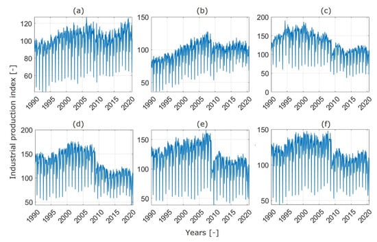
Figure 1.
Historical series of the Italian monthly industrial production index for the (a) Chemicals; (b) Pulp and paper; (c) Non-ferrous metals; (d) Non-metallic minerals; (e) Iron and steel; (f) Other industries subsectors.
To perform accurate projections of the datasets in Figure 1, it is important not only to address the historical trends within each sector, but also to exploit the structural interdependencies among such sectors. This is the main reason to choose a multivariate regression model such as VAR over univariate models such as ARIMA or Exponential Smoothing [29]. The main problem of such models is the over-parameterization derived from the number of variables to be analyzed and the coefficients needed to describe all the relationships among the lagged values. The analysis presented in this work is in principle not exempt from that issue, given the large number of variables to project. In such cases, a sparse VAR modeling approach is very useful [31]. Indeed, it is reasonable that not every coefficient describing the relationship among different lagged values introduces significant information to improve the regression accuracy. In fact, in a sparse VAR model (sVAR) most of the autoregressive coefficients are set equal to zero, and the methods to select which parameters can be set to zero are automatically implemented by the fitting functions in the sparsevar package of the software R, selected here as the computing environment [29].
An important step for the VAR model construction is selecting the best number of lagged variables in the system. Information criteria such as Akaike and Hannan–Quinn criteria (AIC and HQC, respectively) are generally used to select the number of lags to be included and to choose the best regression model. Although, since we are not interested in having a good regression, but we are interested in accurate forecasts, such criteria may not be the best choice [29]. On the other hand, the Bayesian criterion (BIC) is based on log-likelihood function (LLF), similar to AIC, and it is used to measure the predictive ability of different models. Nonetheless, such a criterion heavily penalizes complex models, and this may be a conservative choice for model selection when choosing the number of regression parameters [32]. For such reasons, a cross-validation approach has been used. Cross-validation is widely employed in the regression and prediction of time series to assess the accuracy of a forecast model by averaging predictive errors across mutually exclusive data subsamples. Estimates can then be used to select the most accurate model among multiple candidates [32]. In more detail, a time-series cross-validation procedure based on a rolling forecast origin has been performed [29]. This is an iterative process, where the first iteration has consisted in considering a two-year training set in the period 1990–1991. The test set includes a one-step-ahead forecast (i.e., the projection at January 1992) that represents the starting point for the estimation of a forecast error, performed by comparing the result against historical values. In the second iteration, the training set is increased by one month ahead, and the test set is represented by the forecast for February 1992. This procedure is iterated until the training set corresponds to the last month in the historical dataset. Figure 2 shows the first six steps of the procedure, considering the historical values of the Chemicals industrial production index as an example. It can be clearly seen how the training set for the VAR model selection increases at each iteration, while the test set remains frozen at one step ahead.
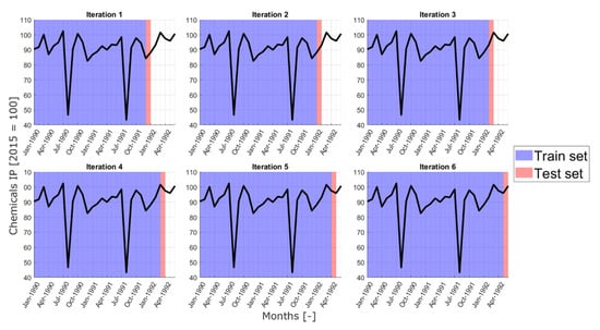
Figure 2.
Cross-validation procedure for model selection. The first six iterations of such a procedure are shown.
The final output of the cross-validation procedure highlighted above is a vector containing the errors computed for the different forecasts, out of which a Root Mean Square Error (RMSE) can be determined, to have a single quantitative evaluation of the overall forecast accuracy of the selected model. RMSE measures the average prediction error made by the model in predicting the outcome for an observation. Therefore, it is defined as the average difference between the observed known outcome values and the values predicted by the model. In fact, the cross-validation has been performed for various VAR models with a different number of lags, and it can be seen that the most accurate model, i.e., the one with the lower RMSE, is the VAR(12) model, as shown in Figure 3. The VAR(12) model is computed using 12 monthly lagged values, confirming then the strong annual seasonality of the time series analyzed.
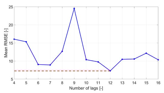
Figure 3.
Selection of the number of lags from RMSE minimization as a function of the number of lagged values.
3. VAR Driver Projection: Results and Discussion
The validation of the forecast model described above has been made by considering the historical series up to 2017 and performing forecasts starting from 2018 up to 2040. As no other source of projections relative to Italy and taking into account the effects of the pandemic is currently available, the projections from in the Italian Integrated National Energy And Climate Plan (PNIEC) [20], which in turn are projections taken from the EU Reference Scenario 2016 [33] (i.e., before the pandemic), have been deemed as the most reliable source of comparison and have been adopted here to validate the computed results.
The results of the validation are reported in Figure 4, Figure 5, Figure 6, Figure 7, Figure 8 and Figure 9, showing the post-2020 projections of the VAR model, along with their 95% confidence bounds.
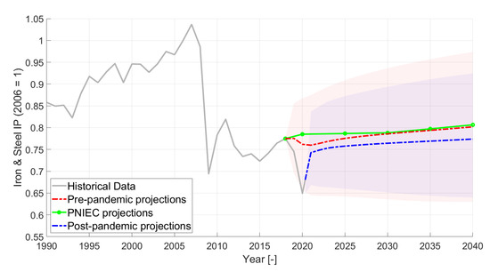
Figure 4.
Iron and steel industrial production projections. The light red area encloses the 95% confidence bound related to the pre-pandemic projections, while the light blue area represents the range enclosed within the 95% confidence bounds related to the post-pandemic projections.
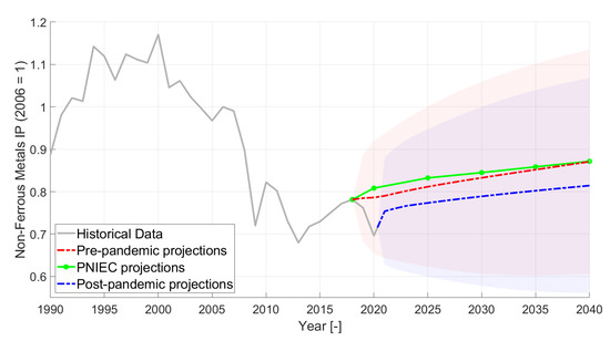
Figure 5.
Non-ferrous metal industrial production projections. The light red area encloses the 95% confidence bound related to the pre-pandemic projections, while the light blue area represents the range enclosed within the 95% confidence bounds related to the post-pandemic projections.
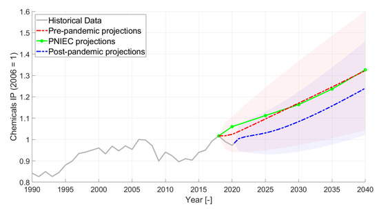
Figure 6.
Chemicals industrial production projections. The light red area encloses the 95% confidence bound related to the pre-pandemic projections, while the light blue area represents the range enclosed within the 95% confidence bounds related to the post-pandemic projections.
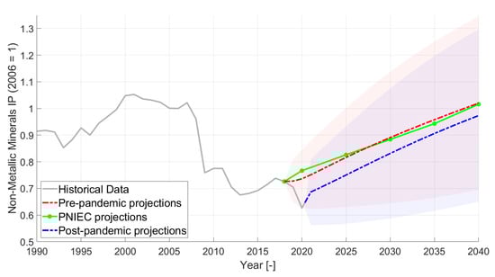
Figure 7.
Non-metallic minerals industrial production projections. The light red area encloses the 95% confidence bound related to the pre-pandemic projections, while the light blue area represents the range enclosed within the 95% confidence bounds related to the post-pandemic projections.
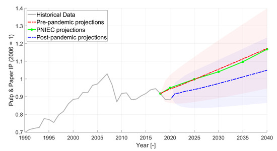
Figure 8.
Pulp, paper and printing industrial production projections. The light red area encloses the 95% confidence bound related to the pre-pandemic projections, while the light blue area represents the range enclosed within the 95% confidence bounds related to the post-pandemic projections.
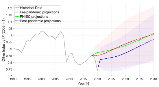
Figure 9.
Other industries industrial production final projections. The light red area encloses the 95% confidence bound related to the pre-pandemic projections, while the light blue area represents the range enclosed within the 95% confidence bounds related to the post-pandemic projections.
Analyzing the results subsector by subsector, Figure 4 shows the projections of iron and steel production, while Figure 5 shows the projections of Non-ferrous metals production. In both cases, the pre-pandemic VAR projections better follow the decreasing trend of the latest years, further dejected by the 2020 economic crisis. On the other hand, both subsector productions show a very similar long-term trend with respect to the ones in the PNIEC scenarios in the pre-pandemic projections.
For iron and steel production in Figure 4, the post-pandemic projections result in a post-crisis recovery that presents the same short-term behavior as in the post-2009 recession. In the long term, a slightly slower increasing trend than the pre-pandemic projections is computed. Note that, despite the growing rate, the production remains significantly smaller than what it was in 2007 (peak level), but post-pandemic projections are able to reach pre-pandemic (2019) historical levels already starting from 2022. For the Non-ferrous metal productions in Figure 5, the post-pandemic projections present again a shock response similar to the one had after the Great Recession. In the long-term there is still an increasing trend, even if it is slower than that of the pre-pandemic projections. Even in this case, the post-pandemic projections are able to reach pre-pandemic historical levels starting from 2022, but the peak production levels of the year 2000 are never reached again.
Eventually, the iron and steel sector in 2040 shows just a −3.5% deviation with respect to PNIEC and pre-pandemic projections, while Non-ferrous metals production in 2040 is computed to be just 6.5% lower than in PNIEC and pre-pandemic projections.
Figure 6 shows the projections for the chemical sector, while the projections of the Non-metallic minerals sector production are reported in Figure 7. Both those sectors present a stronger increasing trend with respect to the iron and steel and Non-ferrous metals, but the computed pre-pandemic VAR projections present, again, a similar behavior to the one discussed above. For Chemicals production, as shown in Figure 6, the post-pandemic projections show a small bouncing effect in the short term, in line with the post-2009 crisis recovery behavior, and no stagnation in the medium term. The pandemic is anticipated to have a very time-limited effect on this set of forecasts, and the growth highlighted by the historical series confirmed both the pre- and post-pandemic projections. The Chemicals sector is the one showing the highest growth rate and the highest absolute growth with respect to the 2006 value, despite the pandemic, but also a wide range between PNIEC/pre-pandemic and post-pandemic projections, with a 6.25% difference. For the Non-metallic minerals production in Figure 7, the short-term bounce is followed by a strong increasing trend, both in the pre-pandemic and the post-pandemic projections. In 2040, the Non-metallic minerals production is anticipated to reach comparable levels with respect to 2006 both in the pre- and post-pandemic projections, with the effects of the pandemic leading to a 4.55% difference in 2040 with respect to the PNIEC/pre-pandemic projections. A steeper growth rate of the post-pandemic projection with respect to the PNIEC/pre-pandemic lines is also visible in the long term.
The results for the pulp, paper and printing sector are presented in Figure 8, and in this case of the pre-pandemic trend, the VAR projections are in line with PNIEC even in the short term. The rest of the industrial production is grouped under “Other industries”, even though it represents an important share of the total Italian industrial production, and the other-industries production trend is shown in Figure 9. The pre-pandemic VAR future projections do not differ much from the results of Non-metallic minerals in Figure 7. The post-pandemic projections for the pulp, paper and printing production in Figure 8 show a smooth recovery from the 2020 decrease. The growth rate is linear and the slope is smaller than the one of the pre-pandemic projections. Such behavior is similar to the chemicals industrial production projection, as expected given the similar historical trends of the two sectors (see Figure 6 and Figure 8). The reason for the lower increase in the projections of Pulp and paper production can be investigated by giving a look at its historical series, and considering that the recovery from the 2009 crisis was very slow. The results of the projections lead to a 10.5% difference between the PNIEC/pre-pandemic and post-pandemic projections in 2040 for the pulp, paper and printing sector. The 2007 peak production is reached and overcome in both pre-pandemic (from 2026 on) and post-pandemic (from 2038 on) projections. In the case of the other industries, a 3.65% smaller industrial production index is computed in 2040 when the effect of the pandemic is considered, and, despite the steeper trend computed in the post-pandemic projections, the 2007 peak production levels are never reached again.
In Table 1, the plotted behavior of the pre-pandemic VAR projections is summarized, translated in terms of average annual growth rates and compared to the annual growth rates of the added values of the industrial sectors in the baseline and PNIEC scenarios, taken as reference for the model validation.

Table 1.
Average annual growth rate of industrial drivers in VAR projections and (in brackets) PNIEC scenarios.
As can be seen from Table 1, the growth rate values computed using VAR present various differences if compared to the PNIEC projections, especially in the short term. Note, however, that the 2019 projections of the VAR model seem globally to better follow the historical decreasing trend, and this good short-term accuracy is important to have reliable forecasts of the post-pandemic recovery. Table 2 shows the absolute values of such projections, in terms of the average annual industrial production index, expressed as industrial output normalized as a base value of 100 at the year 2005. The percentage deviations between the values are also shown, and it can be seen how, in the short term, every VAR projection confirms slightly lower results than the PNIEC values, but such projections are better following the decreasing historical values, as seen in Figure 4, Figure 5, Figure 6, Figure 7, Figure 8 and Figure 9. In any case, the relative difference between the VAR projection and the PNIEC ones is lower than 1.5%. In the long term, all the computed results tend to get closer to the reference projections, with a very small difference in 2040 (<0.8%) with respect to the PNIEC values.
Table 2.
Average annual industrial production projections according to the VAR model adopted in this paper (pre-pandemic projections) and PNIEC projections (base 2015 = 100), along with the percentage deviation of the VAR values with respect to PNIEC estimates.
Table 3 represents the industrial production VAR projections with and without the 2020 pandemic effects. Overall, all the industrial sectors seem to be affected by the crisis, but with different amplitudes, both in the short and long term. In fact, sectors such as Chemicals and Pulp and paper react to the pandemic with a smaller reduction, with respect to the pre-pandemic expectations, if compared to the other subsector. However, in the long term they show a smaller capability to react to the crisis (especially the Pulp, paper and printing sector). In more detail, the Iron and steel and Non-ferrous metals show just a slightly slower increase in the production index, if compared to the pre-pandemic situation. The Non-metallic minerals and the Other industries subsectors increase more steeply in the medium-long term than foreseen before the pandemic in the medium-long term. The main shift in the post-pandemic projections concerns the Pulp, paper and printing sector, which presents in the long run a much lower increase if compared to the pre-pandemic expectations, possibly highlighting some structural change in the industrial production.
Table 3.
Average annual values of the monthly industrial production index (base 2015 = 100) in the post-pandemic projections, together with the absolute difference computed between the post- and pre-pandemic projections (Δ) in the short, medium and long term.
The differences between pre- and post-pandemic projections for the different subsectors in Table 3, as well as in Figure 4, Figure 5, Figure 6, Figure 7, Figure 8 and Figure 9, are mostly related to the reductions registered in 2019 with respect to 2018. In fact, on the one hand, the pre-pandemic projections do not completely catch such a reduction in 2019, and on the other hand post-pandemic projections present an almost full recovery, with 2021 values close to 2019. The Pulp and paper sector is the only exception in terms of a significantly lower long-term trend in the post-pandemic results compared to pre-pandemic. This is mostly due to the autoregressive nature of VAR models, where a longer post-2009 crisis stagnation up to 2021 has led to less optimistic results with respect to pre-pandemic projections.
4. Effect of VAR Driver Projections in the Evolution of the Italian Industrial Sector
Once the industrial production projections are computed via VAR models and validated against PNIEC projections, their application to an energy system modeling framework is presented here, using the TIMES-Italy model mentioned in the introduction and focusing on the outcomes for the Italian industrial sector. Unfortunately, no comparison with other published works is currently possible, due to the absence of similar published analyses, especially concerning the very circumstantiated case of the Italian industrial sector.
Both pre-pandemic and post-pandemic industrial production projections are adopted as drivers in Equation (1) for the calculation of the energy service demand for the Italian RES throughout a time scale from 2006 to 2040. The time horizon is divided into a user-chosen number of time-periods, each period containing a (possibly different) number of years, which are then identified according to a single milestone year per period [2]. The current version of TIMES-Italy is characterized by time intervals with increasing amplitude: the first two periods represent single years, then the duration of each time step increases to two years until 2022, to five years between 2025 and 2030, and to ten years between 2030 and 2040. Therefore, the identified milestone years are: 2006, 2007, 2008, 2010, 2012, 2014, 2016, 2018, 2020, 2022, 2025, 2030, and 2040. For this reason, all drivers but those of the industrial sector are projected according to PNIEC results. As TIMES interpolates the user-defined timeseries data (including drivers) only for the milestone years, and then uses the value at the milestone year as a representative value for the whole period [2], the computed industrial production rates are averaged to representative values for each milestone year in order to be used in TIMES-Italy.
The results from a business as usual (BAU) scenario are presented, without considering the adoption of any particular policy measure neither to contrast the increase in CO2 emission nor any limitation on the use of specific energy carriers, e.g., coal and gas, just to show the effects of the modified drivers on the energy consumption pattern when applied to TIMES-Italy.
Figure 10 presents the total energy consumption patterns in the six Italian industrial subsectors modeled in TIMES-Italy and the whole industry sector.
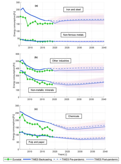
Figure 10.
Energy consumption back-casting and forecasting for the (a) Iron and steel, Non-ferrous metals; (b) Other industries, Non-metallic minerals; and (c) Chemicals, Pulp and paper subsectors using TIMES-Italy. The TIMES-Italy back-casting is benchmarked against Eurostat historical series 2006–2019. Projections obtained using the upper and lower bounds of the 95% confidence interval as drivers are enclosed within the light red (pre-pandemic) and light blue (post-pandemic) areas.
For the period 2006–2019, a benchmark of the computed results against Eurostat historical series is possible, and it is shown that most of the sectors present the same (or very similar) starting point for energy consumption in 2006 (Non-ferrous metals in Figure 10a, Other industries and Non-metallic minerals in Figure 10b, and Pulp and paper in Figure 10c) and comparable trends, confirming the reliability of the TIMES-Italy as a forecasting tool for those subsectors. On the other hand, wide inconsistencies are highlighted in the Iron and steel and Chemicals subsector in Figure 10a,c, for which TIMES-Italy overestimates energy consumption starting levels. The difference throughout the whole back-casting time scale is also reflected in Figure 11 for the total industrial energy consumption. In Figure 10a for the Iron and steel subsector, the initial 45 PJ difference in 2006 reduced along the years due to the strongly decreasing energy consumption trend, resulting from the uptake of the electric arc furnace for steel production. In the Chemicals sector, the initial 39 PJ difference between Eurostat and the TIMES-Italy consumption in 2006 is broadened due to the lower decreasing rate in energy consumption in TIMES-Italy. The main reason for the different starting points is to be found in the change of the accounting method for the compilation of Eurostat energy balances. Indeed, TIMES-Italy calibration was performed using the 2009 version of the IEA energy balances for OECD countries [23], before the update in their accounting methodology.
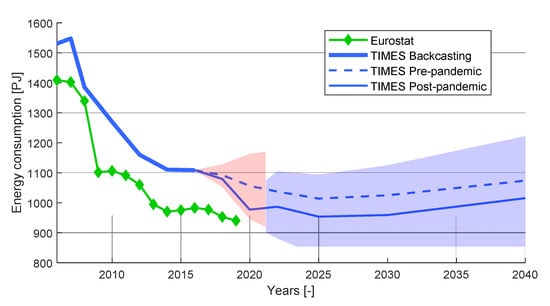
Figure 11.
Energy consumption back-casting and projections for the whole Italian industrial sector. using TIMES-Italy. The TIMES-Italy back-casting is benchmarked against Eurostat historical series 2006–2019.
Looking now at the forecasts in Figure 10, the first and expected outcome is that a lower energy consumption correspond to the lower demand obtained in the post-pandemic projections of industrial productions. Even though the economic shock caused by the pandemic shows its effects in most subsectors, according to the strong bump highlighted in Figure 4, Figure 5, Figure 6, Figure 7, Figure 8 and Figure 9 in the 2020 levels of industrial production, the energy consumption reduction due to the use of post-pandemic drivers is almost imperceptible in the Iron and steel subsector (Figure 10a), also considering that demand growth in that sector after 2025 (see Figure 4) is not dramatic. The low energy consumption level of the Non-ferrous metals subsector (always < 50 PJ) shows an almost negligible difference in the two alternative projection sets (see Figure 10a). In Figure 10b, the Non-metallic minerals, notwithstanding the demand gap between the pre-pandemic and post-pandemic projections highlighted in Figure 7, present a difference of just 4% when it comes to energy consumption. On the other hand, it is interesting to notice how the optimization process encompassed in TIMES can lead to a stronger energy consumption reduction in the Chemical sector, where demand growth, even when considering post-pandemic drivers, leads to a large growth with respect to 2006 levels. However, such a strong demand growth (Figure 6) is reflected on an energy consumption level, which is 40% and 36% lower in 2040 with respect to 2006 for post-pandemic and pre-pandemic projections, respectively.
Eventually, concerning total industrial energy demand in Figure 11, the 7% (79 PJ) energy consumption range between the pre- and post-pandemic driver projections for the year 2020 thins to 59 PJ in 2040, but showing a generally increasing trend that is very slow if compared to a steep demand growth in all sectors except Chemicals.
In Figure 12, the detailed industrial energy mix at three selected time steps (2006, the base year; 2020 and 2040) is shown, using pre-pandemic and post-pandemic drivers in 2020 and 2040. It is evident how the application of the TIMES cost optimization algorithm, coupled to the availability of more efficient technologies in the years following 2006, has the greatest impact on the modifications to the energy mix. Indeed, the decreasing energy demand is mostly due to a steep decline (>60% in the two cases) in oil product consumption from 2006 to 2020. Moreover, natural gas shows a considerable decline (40%) from 2006 to 2020, while the use of biomass is more than doubled, but still negligible with respect to the other sources. The analyzed scenario being a business-as-usual case study in which innovative low-carbon technological options can be adopted, but without considering, e.g., the application of carbon capture and storage (CCS) or the prescription of any CO2 emission target, the energy mix in 2040 practically stays the same as in 2020. Nonetheless, coal is the only one among fossil fuels showing a substantial growth (>90% in both cases using pre- and post-pandemic driver projections), which is mainly due to the considerable uptake of the highly efficient and cost-effective HIsarna-BOF steel production technology [34] and the displacement in fuel use for clinker production in the Non-metallic minerals sectors, where oil is almost totally replaced by coal.
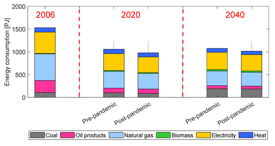
Figure 12.
Energy consumption mix at three selected time steps, as computed by TIMES-Italy.
Comparing in Figure 12 the prediction including or not including the pandemic effect, no substantial structural change in the energy mix behind the industry sector is observed just as an effect of the pandemic, suggesting that no significant structural change in the industry sector has been induced.
5. Conclusions
A new VAR model has been developed here to project the whole set of industrial energy service demands for the Italian industry sector, based on the detailed analysis of the seasonal historical consumption dataset. In a first case, where the reference dataset for the projection development did not include the pandemic period, the VAR model allowed for computing demand projections in line with those from PNIEC, without the need to rely on macro-economic complex tools. The use of regression models such as VAR is shown then to be a valid tool for obtaining reliable forecasts in cases where unexpected events (such as the pandemic crisis) make the picture depicted by macroeconomic models out of date. When considering the effects of the pandemic in the long term, most industrial sectors show a slower decrease than that computed before the pandemic, and, among them, the Pulp and paper subsector is anticipated to have a significant slow-down in the next 15 years.
When the industrial production trends computed using the developed VAR model are applied to the Italian energy system in the long run using the TIMES-Italy modeling framework, in a business-as-usual scenario, the effects of the pandemic affect the long-term energy consumption in the industrial sector with a decrease in the overall energy consumption of ~5% (60 PJ) throughout the entire time horizon to 2040. The computed energy mix composition does not show dramatic changes in 2040 with respect to 2020. Furthermore, in the BAU scenario analyzed here, no significant structural impact of the pandemic has been computed for the industry sector.
Author Contributions
Conceptualization, A.O., F.G., D.L., M.N. and L.S.; methodology, A.O., D.L. and M.N.; software, A.O.; validation, A.O., D.L. and M.N.; formal analysis, A.O., F.G., D.L., M.N. and L.S.; investigation, D.L.; resources, D.L. and M.N.; data curation, A.O. and D.L.; writing—original draft preparation, A.O., D.L. and M.N..; writing—review and editing, F.G. and L.S.; visualization, A.O., D.L. and L.S.; supervision, L.S.; project administration, L.S..; funding acquisition, L.S. All authors have read and agreed to the published version of the manuscript.
Funding
This research received no external funding.
Conflicts of Interest
The authors declare no conflict of interest.
References
- DeCarolis, J.; Hunter, K.; Sreepathi, S. The case for repeatable analysis with energy economy optimization models. Energy Econ. 2012, 34, 1845–1853. [Google Scholar] [CrossRef]
- Loulou, R.; Goldstein, G.; Kanudia, A.; Lettila, A.; Remme, U. Documentation for the TIMES model: Part I; IEA-ETSAP: Paris, France, 2016. [Google Scholar]
- Ekholm, T.; Lehtilä, A. EFDA-TIMES Model Industry Update; VTT Energy System: Espoo, Finland, 2008. [Google Scholar]
- E3MLab/ICCS at National Technical University of and Athens. PRIMES Model. 2014. Available online: https://ec.europa.eu/clima/sites/clima/files/strategies/analysis/models/docs/primes_model_2013-2014_en.pdf (accessed on 1 September 2021).
- Simoes, S.; Nijs, W.; Ruiz, P.; Sgobbi, A.; Radu, D.; Bolat, P.; Thiel, C.; Peteves, S. The JRC-EU-TIMES Model; Assessing the long-term role of the SET Plan Energy technologies, no. EUR 26292 EN; Publications Office of the European Union: Luxembourg, 2013. [Google Scholar]
- EUROfusion. EUROfusion Collaborators—Socio Economic Studies; EUROfusion: Garching, Germany, 2021; Available online: https://collaborators.euro-fusion.org/collaborators/socio-economic-studies/ (accessed on 1 September 2021).
- ORDECSYS; KanORS; HALOA; KUL. EFDA World TIMES Model. 2004. Available online: https://www.euro-fusion.org/fileadmin/user_upload/Archive/wp-content/uploads/2014/12/R37EFDA-final-report_oct_14.pdf (accessed on 1 September 2021).
- Capros, P.; Van Regenmorter, D.; Paroussos, L.; Karkatsoulis, P.; Fragkiadakis, C.; Tsani, S.; Charalampidis, I.; Revesz, T. GEM-E3 Model Documentation; Publications Office of the European Union: Luxembourg, 2013. [Google Scholar]
- International Energy Agency (IEA). Global Energy Review 2020; IEA: Paris, France, 2020. [CrossRef]
- IEA. World Energy Outlook 2020; IEA: Paris, France, 2020.
- Kennedy, S. G-20’s Economy Returns to Pre-Pandemic Level, But Gaps Linger. Bloomberg 2021. Available online: https://www.bloomberg.com/news/articles/2021-06-10/g-20-s-economy-returns-to-pre-pandemic-level-but-gaps-linger (accessed on 1 September 2021).
- Pizzoli, P. Italian industrial production back to pre-pandemic levels. ING Econ. Financ. Anal. 2021. Available online: https://think.ing.com/articles/italy-industrial-production-accelerated-substantially-already-in-april/ (accessed on 1 September 2021).
- Neumann, J.; Goyeneche, A. Italy, Spain Economies Set to Expand at Fastest Rate Since 1970s. Bloomberg 2021. Available online: https://www.bloomberg.com/news/articles/2021-08-16/italy-spain-economies-set-to-expand-at-fastest-rate-since-1970s (accessed on 1 September 2021).
- Zhang, R.; Zhang, J. Long-term pathways to deep decarbonization of the transport sector in the post-COVID world. Transp. Policy 2021, 110, 28–36. [Google Scholar] [CrossRef] [PubMed]
- OECD. The Long-Term Environmental Implications of COVID-19. 2021. Available online: https://www.oecd.org/coronavirus/policy-responses/the-long-term-environmental-implications-of-covid-19-4b7a9937/ (accessed on 1 September 2021).
- Jiang, P.; van Fan, Y.; Klemeš, J.J. Impacts of COVID-19 on energy demand and consumption: Challenges, lessons and emerging opportunities. Appl. Energy 2021, 285, 116441. [Google Scholar] [CrossRef] [PubMed]
- Abu-Rayash, A.; Dincer, I. Analysis of the electricity demand trends amidst the COVID-19 coronavirus pandemic. Energy Res. Soc. Sci. 2020, 68, 101682. [Google Scholar] [CrossRef] [PubMed]
- Norouzi, N.; de Rubens, G.Z.; Choupanpiesheh, S.; Enevoldsen, P. When pandemics impact economies and climate change: Exploring the impacts of COVID-19 on oil and electricity demand in China. Energy Res. Soc. Sci. 2020, 68, 101654. [Google Scholar] [CrossRef] [PubMed]
- Foroni, C.; Marcellino, M.; Stevanovic, D. Forecasting the Covid-19 recession and recovery: Lessons from the financial crisis. Int. J. Forecast. 2020. [Google Scholar] [CrossRef]
- Ministry of Economic Development; Ministry of the Environment and Protection of Natural Resources and the Sea; Ministry of Infrastructure and Transport. Integrated National Energy and Climate Plan; 2019. Available online: https://www.mise.gov.it/images/stories/documenti/it_final_necp_main_en.pdf (accessed on 1 September 2021).
- Gaeta, M.; Baldissara, B. IL MODELLO ENERGETICO TIMES-Italia Struttura e Dati; ENEA: Rome, Italy, 2011. [Google Scholar]
- Ministry of the Environment and Protection of Natural Resources and the Sea. Strategia Energetica Nazionale (SEN), 2017; 2017. Available online: https://www.mise.gov.it/images/stories/documenti/Testo-integrale-SEN-2017.pdf (accessed on 1 September 2021).
- OECD-IEA. Energy Balances of OECD Countries, 2009 ed.; 2009; Available online: https://www.oecd-ilibrary.org/energy/energy-balances-of-oecd-countries-2009_energy_bal_oecd-2009-en-fr (accessed on 1 September 2021).
- ISTAT. Istat Statistics—ICT Indicators; 2017. Available online: http://dati.istat.it/Index.aspx?DataSetCode=DCSC_ORDFATT&Lang=EN# (accessed on 1 September 2021).
- Hunt, L.C.; Ryan, D.L. Economic modelling of energy services: Rectifying misspecified energy demand functions. Energy Econ. 2015, 50, 273–285. [Google Scholar] [CrossRef] [Green Version]
- Kilian, L. Handbook of Research Methods and Applications in Empirical Macroeconomics; Edward Elgar: Cheltenham, UK, 2015. [Google Scholar]
- Sims, C.A. Macroeconomics and Reality. Econometrica 1980, 48, 1. [Google Scholar] [CrossRef] [Green Version]
- Chen, P.; Frohn, J. On the Specification and Estimation of Large Scale Simultaneous Structural Models; Springer: Berlin, Germany, 2006. [Google Scholar]
- Hyndman, R.J.; Athanasopoulos, G. Forecasting: Principles and Practice, 3rd ed.; OTexts: Melbourne, Australia, 2021; Available online: https://otexts.com/fpp3/ (accessed on 17 February 2021).
- Draper, N.R.; Smith, H. ‘Dummy’ Variables. Appl. Regres. Anal. 1998, 299–325. [Google Scholar] [CrossRef]
- Sims, C.A.; Zha, T. Bayesian Methods for Dynamic Multivariate Models. Int. Econ. Rev. (Phila.) 1998, 39, 949. [Google Scholar] [CrossRef] [Green Version]
- Stone, M. Cross-Validatory Choice and Assessment of Statistical Predictions. J. R. Stat. Soc. Ser. B 1974, 36, 111–147. Available online: http://www.jstor.org/stable/2984809 (accessed on 1 September 2021). [CrossRef]
- European Commission. EU Reference Scenario 2016. EU Ref. Scenar. 2016, 2016, 27. Available online: https://ec.europa.eu/energy/sites/ener/files/documents/ref2016_report_final-web.pdf (accessed on 1 September 2021).
- Lerede, D.; Bustreo, C.; Gracceva, F.; Saccone, M.; Savoldi, L. Techno-economic and environmental characterization of industrial technologies for transparent bottom-up energy modeling. Renew. Sustain. Energy Rev. 2021, 140, 110742. [Google Scholar] [CrossRef]
Publisher’s Note: MDPI stays neutral with regard to jurisdictional claims in published maps and institutional affiliations. |
© 2021 by the authors. Licensee MDPI, Basel, Switzerland. This article is an open access article distributed under the terms and conditions of the Creative Commons Attribution (CC BY) license (https://creativecommons.org/licenses/by/4.0/).