
A Robust Optimization Approach for Optimal Power Flow Solutions Using Rao Algorithms

 , ,
, , 

Abstract
:1. Introduction
- To develop Rao algorithms to solve OPF problems with six objective functions, namely FCM, VSE under normal and contingency conditions, VPI, RPLM, and ECM.
- To apply Rao algorithms to solve various multi-objective OPF problems by transforming the multi-objective OPF problem into a single objective OPF problem using weighing factors.
- To check the efficiency and supremacy of Rao algorithms by applying these algorithms to solve the OPF problem in three standard IEEE (30-bus, 57-bus, and 118-bus) test systems.
- To compare the simulation outcomes acquired by Rao algorithms for the above-mentioned objective functions with the results of other methods mentioned in recent literature.
- The OPF results demonstrate that the suggested Rao algorithms are efficient and robust in most of the cases over other popular methods, which are reported in recent literature.
2. Problem Formulation
Constraints
- (a)
- Equality Constraints
- (b)
- Inequality Constraints
- Generator Constraints:
- Shunt VAR compensator constraints:
- Transformer Constraints:
- Security Constraints:
- (c)
- Incorporation of Constraints
3. Rao Algorithms
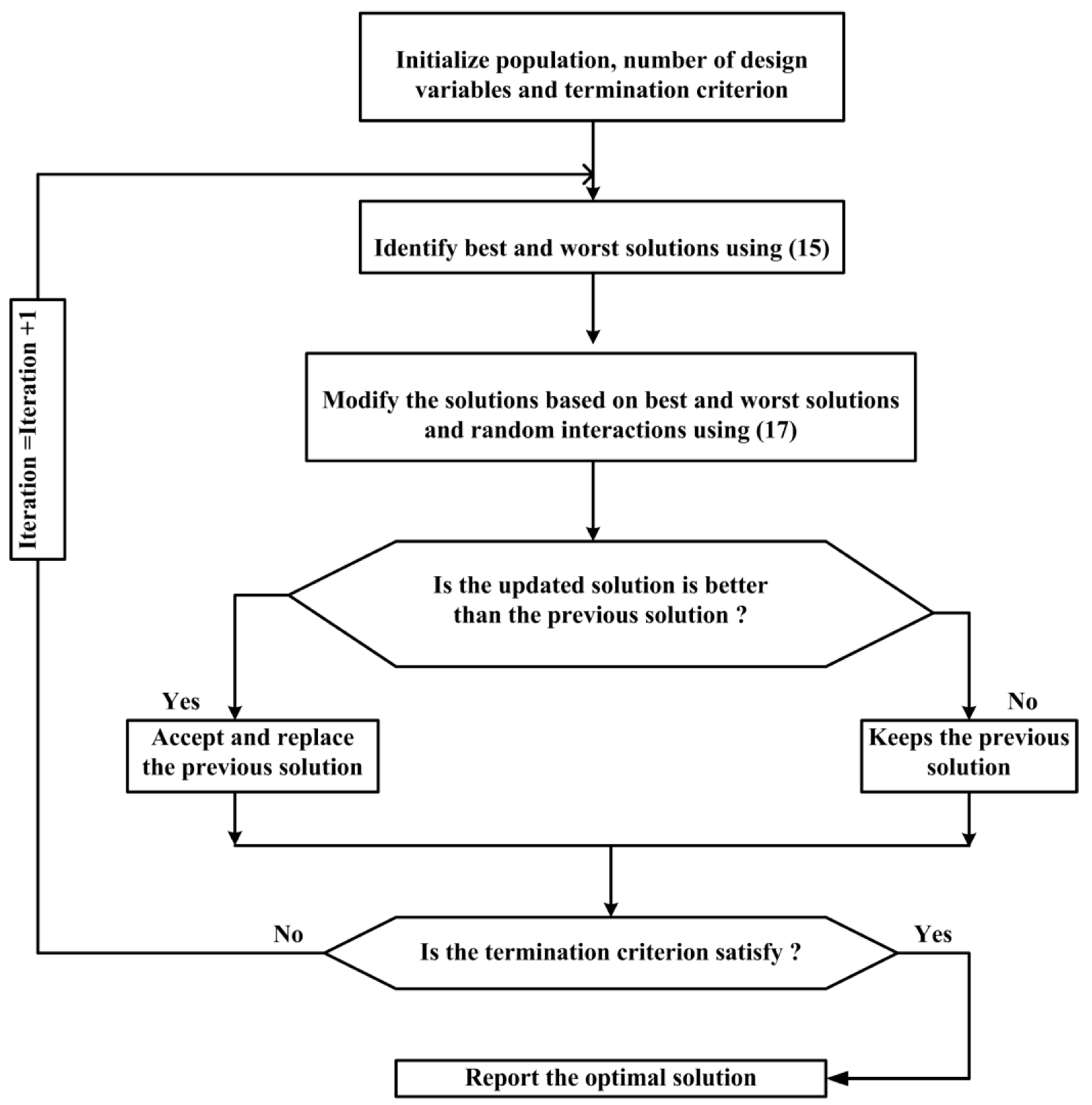
Computational Steps of Rao Algorithms for the OPF Problem
- Randomly generate the initial population with control variables and set the stopping criteria, i.e., It_max.
- Set iterations count to It = 0.
- Identify the worst and best solutions in the population by observing the value of the augmented objective function (15).
- Update the solutions based on the worst and best solutions (17).
- Proceed to step 6 if the updated solution is better than the previous solution; otherwise, proceed to step 7.
- Replace the old solution with the new one. Go to step 8.
- Keep the old solution.
- If It < It_max, increase the count of iteration (i.e., It = It + 1) by 1 and go to step 3. Otherwise go to step 9.
- Stop and display objective function value of best results.
4. OPF Results and Discussion
4.1. IEEE 30-Bus Test System
4.1.1. Case 1: Fuel Cost Minimization (FCM)
4.1.2. Case 2: Voltage Profile Improvement (VPI)
4.1.3. Case 3: Voltage Stability Enhancement (VSE)
4.1.4. Case 4: Voltage Stability Enhancement (VSE) during Contingency
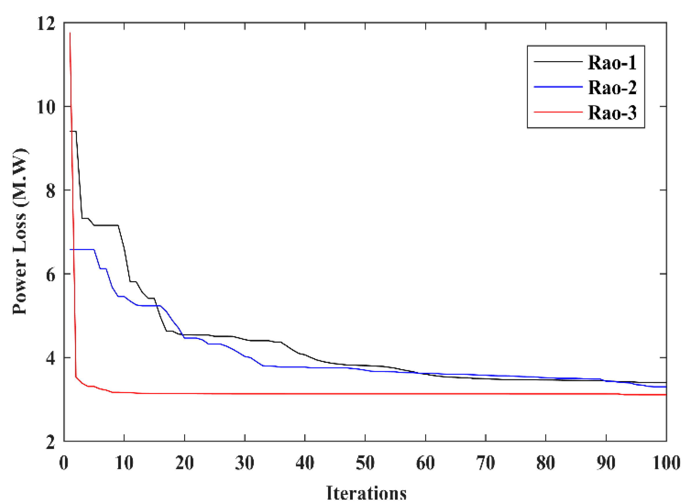
4.1.5. Case 5: Real Power Loss Minimization (RPLM)
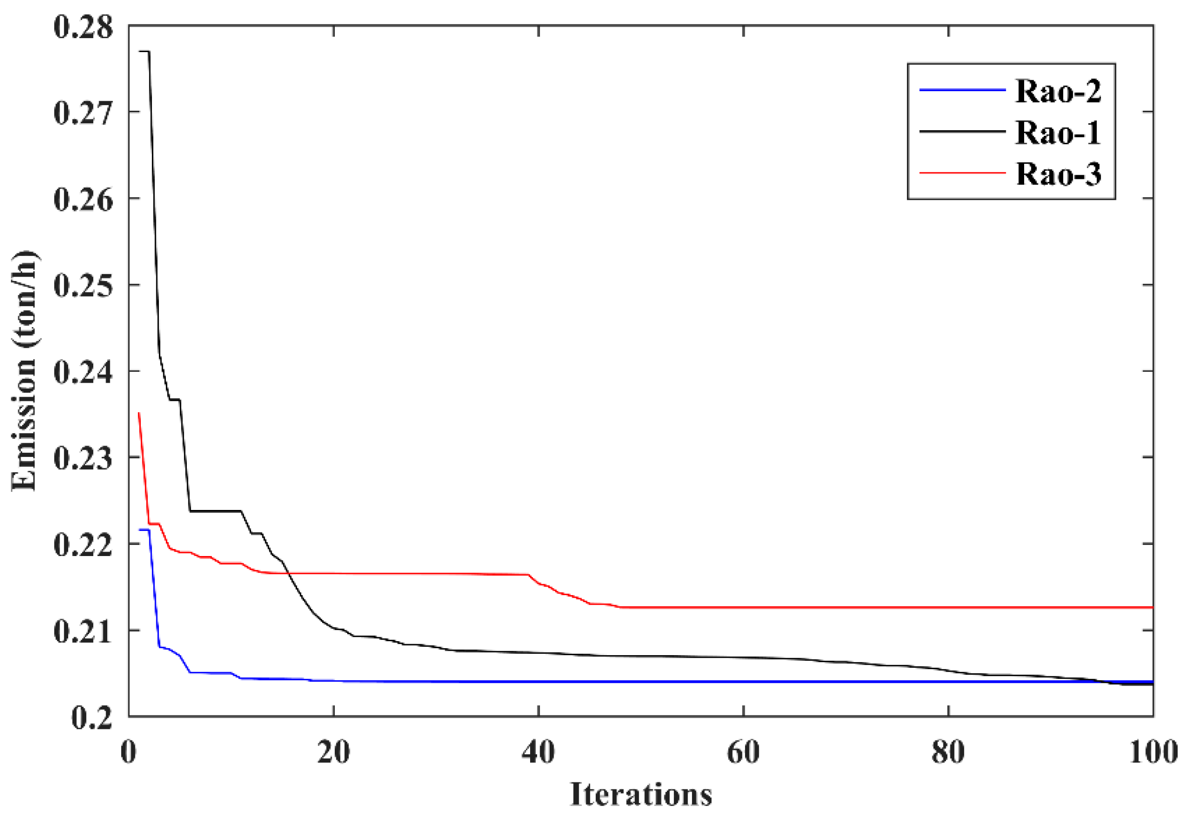
4.1.6. Case 6: Emission Cost Minimization
4.2. IEEE 57-Bus System
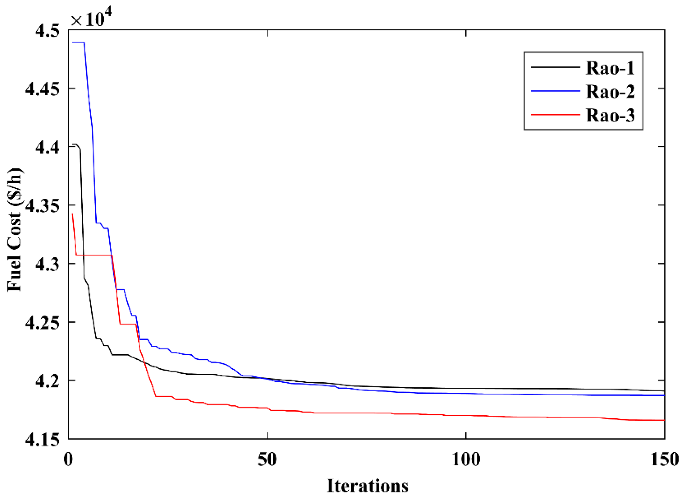
4.2.1. Case 7: Fuel Cost Minimization (FCM)
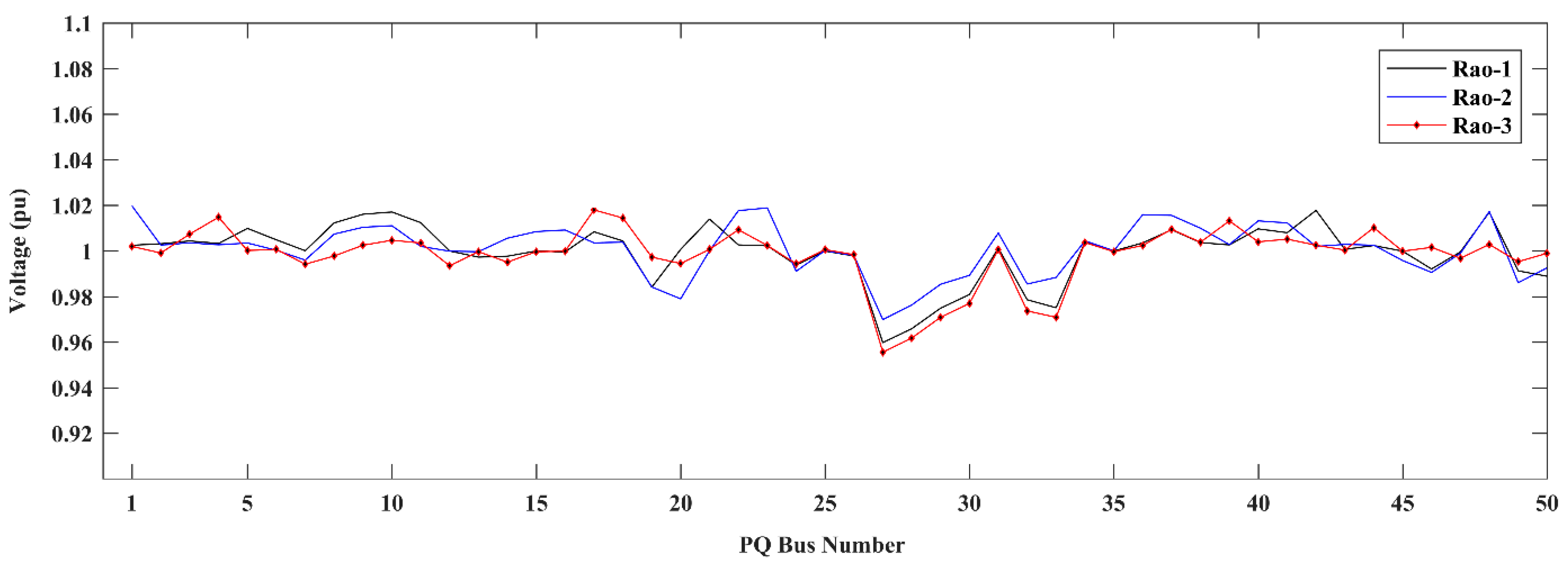
4.2.2. Case 8: Voltage Profile Improvement (VPI)
4.2.3. Case 9: Voltage Stability Enhancement (VSE)
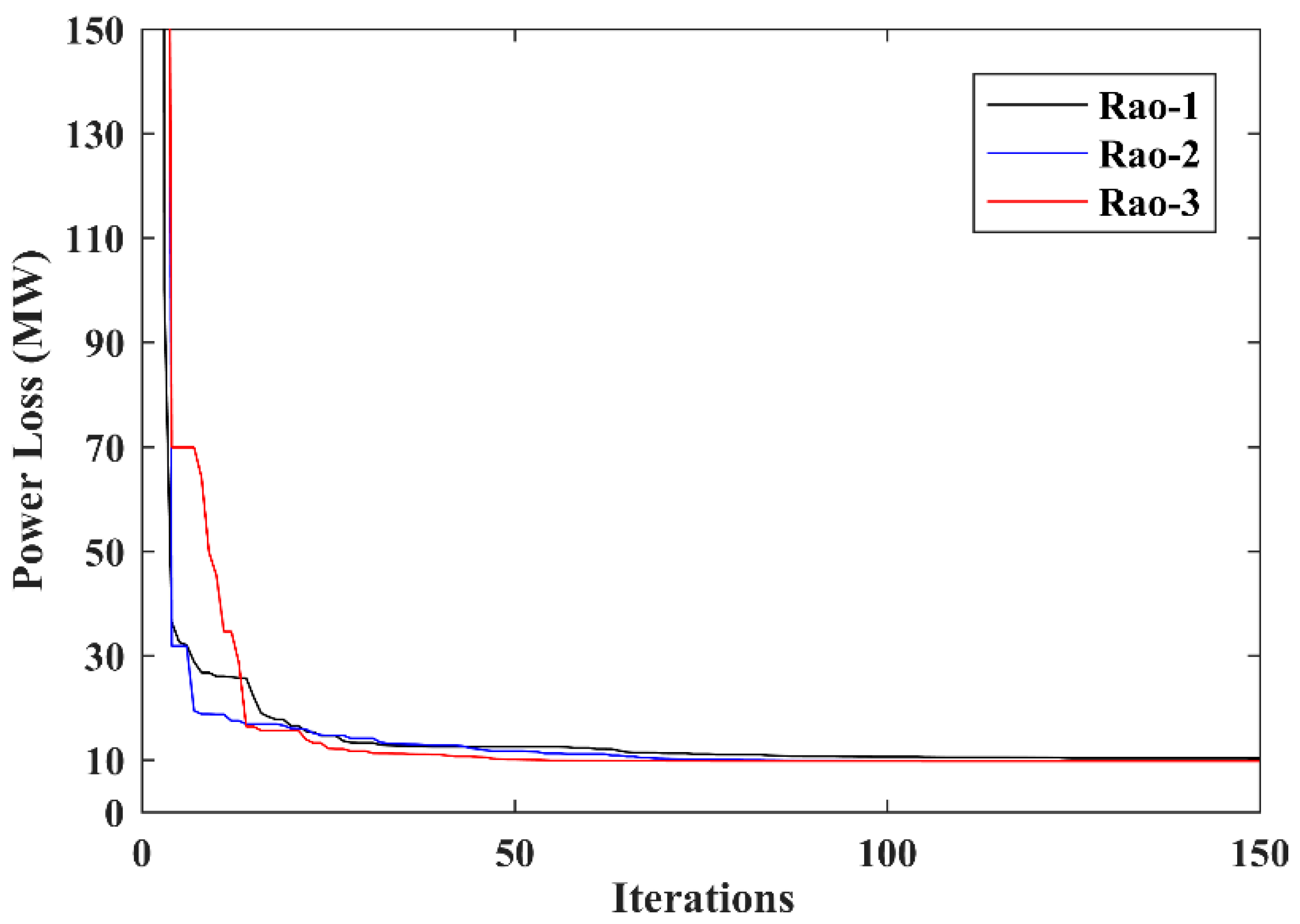
4.2.4. Case 10: Real Power Loss Minimization (RPLM)
4.3. IEEE 118-Bus System
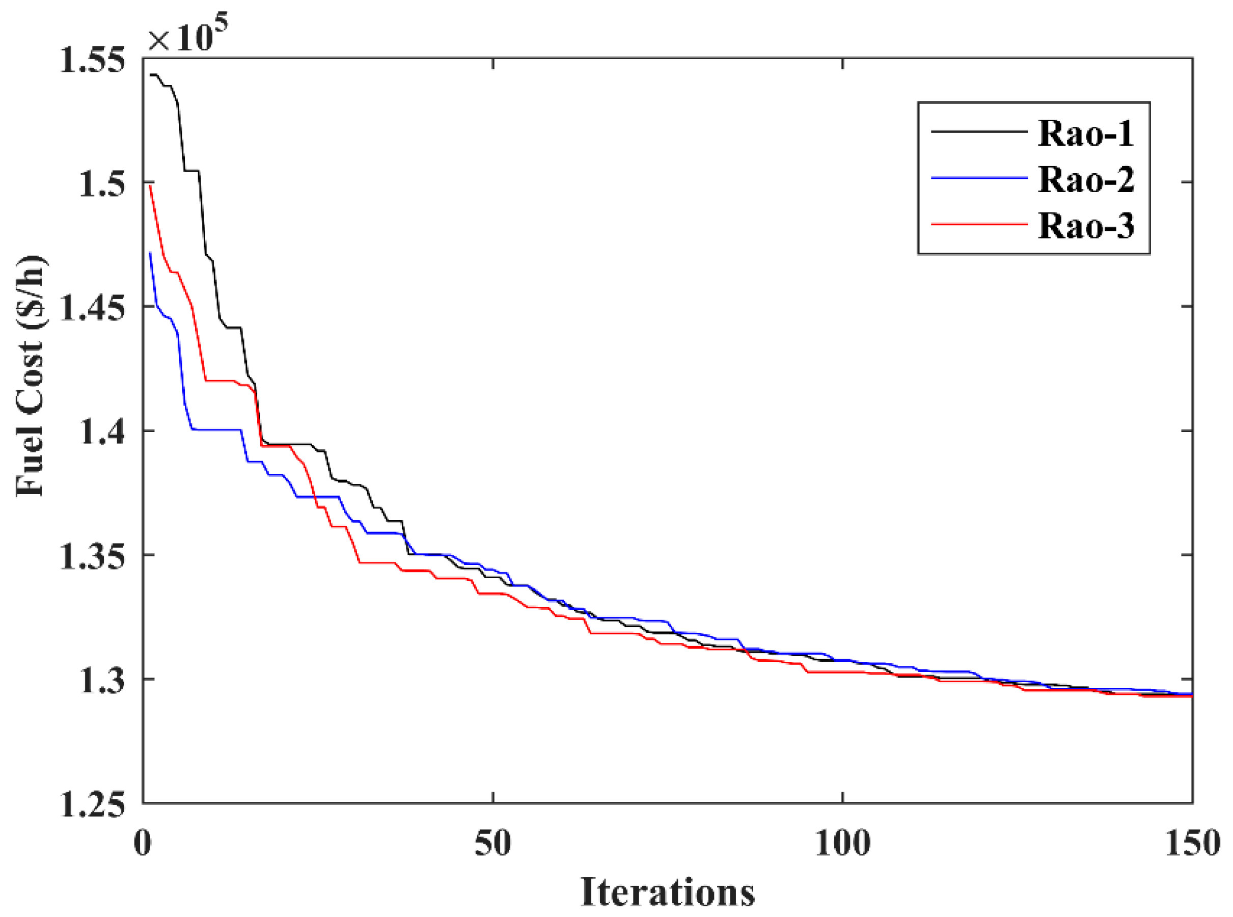
Case 11: Fuel Cost Minimization (FCM)
5. Statistical Comparison of Rao-1, Rao-2, and Rao-3
6. Conclusions
Author Contributions
Funding
Institutional Review Board Statement
Informed Consent Statement
Conflicts of Interest
Nomenclature
| m | state variables |
| n | control variables |
| objective function | |
| g (m, n) | equality constraint |
| h (m, n) | inequality constraint |
| are generator active and reactive power | |
| Nbus | are the set of the bus |
| NLB | are the set of the load bus |
| Ntl | are the set of the transmission line |
| NGN | are the set of generators units |
| NC | are the set shunt compensation switch |
| NTR | are the set of regulating transformers |
| are the load buses’ active and reactive power demand | |
| and | are the total real and reactive power loss |
| and | are maximum and minimum bus voltage limit of the kth generator bus |
| and | are the maximum and minimum limit of the reactive power output of the kth generator bus |
| and | are the maximum and minimum active power limit of the kth generating units |
| and | are the lower and upper voltage limit of the tap setting of the kth transformer |
| and | are the lower and upper voltage limit of the kth load bus |
| is the maximum MVA flow in the kth branch | |
| , , | are the penalty factors |
| , , and | are the ith generator units’ fuel cost coefficients |
| , , , | are the emission coefficients of the ith generator unit |
| PD | active power load demand |
| NB | total number of buses |
| MPSO | modified particle swarm optimization |
| MDE | modified differential evolution |
| MFO | moth flame optimization |
| FPA | flower pollination algorithm |
| QOJA | quasi-oppositional-based Jaya algorithm |
| IMFO | improved moth-flame optimization |
| ARCBBO | adaptive real-coded biogeography-based optimization |
| RCBBO | real-coded biogeography-based optimization |
| GWO | gray wolves optimization |
| MGBICA | multi-objective gaussian bare-bones imperialist competitive algorithm |
| GBICA | gaussian bare-bones imperialist competitive algorithm |
| ABC | artificial bee colony algorithm |
| SKH | stud krill herd algorithm |
| ECHT-DE | ensemble of constraint handling techniques—differential evolution |
| SF-DE | the superiority of feasible solutions–differential evolution |
| SP-DE | self-adaptive penalty–differential evolution |
| MGOA | modified grasshopper optimization algorithm |
| GOA | grasshopper optimization algorithm |
| GPU-PSO | graphics processing unit’s particle swarm optimization |
| ALC-PSO | particle swarm optimization with aging leader and challengers |
| PSOGSA | hybrid particle swarm optimization and gravitational search algorithm |
References
- Roberge, V.; Tarbouchi, M.; Okou, F. Optimal power flow based on parallel metaheuristics for graphics processing units. Electr. Power Syst. Res. 2016, 140, 344–353. [Google Scholar] [CrossRef]
- Saha, A.; Chakraborty, A.K.; Das, P. Quasi-reaction-based symbiotic organisms search algorithm for solving static optimal power flow problem. Sci. Iran. 2019, 26, 1664–1689. [Google Scholar] [CrossRef] [Green Version]
- Carpentier, J. Optimal power flows. Int. J. Electr. Power Energy Syst. 1979, 1, 3–15. [Google Scholar] [CrossRef]
- Maskar, M.B.; Thorat, A.R.; Korachgaon, I. A review on optimal power flow problem and solution methodologies. In Proceedings of the International Conference on Data Management, Analytics and Innovation (ICDMAI), Pune, India, 24–26 February 2017; pp. 64–70. [Google Scholar] [CrossRef]
- Momoh, J.A.; Adapa, R.; El-Hawary, M.E. A review of selected optimal power flow literature to 1993. I. Nonlinear and quadratic programming approaches. IEEE Trans. Power Syst. 1999, 14, 96–104. [Google Scholar] [CrossRef]
- Niu, M.; Wan, C.; Xu, Z. A review on applications of heuristic optimization algorithms for optimal power flow in modern power systems. J. Mod. Power Syst. Clean Energy 2014, 2, 289–297. [Google Scholar] [CrossRef] [Green Version]
- Al Rashidi, M.R.; El-Hawary, M.E. Applications of computational intelligence techniques for solving the revived optimal power flow problem. Electr. Power Syst. Res. 2009, 79, 694–702. [Google Scholar] [CrossRef]
- Gupta, S.; Kumar, N.; Srivastava, L. Bat Search Algorithm for Solving Multi-Objective Optimal Power Flow Problem. In Applications of Computing, Automation and Wireless Systems in Electrical Engineering. Lecture Notes in Electrical Engineering; Springer: Singapore, 2019; Volume 553. [Google Scholar] [CrossRef]
- Bouchekara, H.R.E.H.; Chaib, A.E.; Abido, M.A.; El-Sehiemy, R.A. Optimal power flow using an Improved Colliding Bodies Optimization algorithm. Appl. Soft Comput. J. 2016, 42, 119–131. [Google Scholar] [CrossRef]
- Bouchekara, H.R.E.H. Optimal power flow using black-hole-based optimization approach. Appl. Soft Comput. J. 2014, 24, 879–888. [Google Scholar] [CrossRef]
- Sivasubramani, S.; Swarup, K.S. Multiagent based differential evolution approach to optimal power flow. Appl. Soft Comput. J. 2012, 12, 735–740. [Google Scholar] [CrossRef]
- Daryani, N.; Hagh, M.T.; Teimourzadeh, S. Adaptive group search optimization algorithm for multi-objective optimal power flow problem. Appl. Soft Comput. J. 2016, 38, 1012–1024. [Google Scholar] [CrossRef]
- Roy, P.K.; Ghoshal, S.P.; Thakur, S.S. Multi-objective Optimal Power Flow Using Biogeography-based Optimization. Electr. Power Compon. Syst. 2010, 38, 1406–1426. [Google Scholar] [CrossRef]
- Mohamed, A.A.A.; Mohamed, Y.S.; El-Gaafary, A.A.M.; Hemeida, A.M. Optimal power flow using moth swarm algorithm. Electr. Power Compon. Syst. 2017, 142, 190–206. [Google Scholar] [CrossRef]
- Saha, A.; Das, P.; Chakraborty, A.K. Water evaporation algorithm: A new metaheuristic algorithm towards the solution of optimal power flow. Eng. Sci. Technol. Int. J. 2017, 20, 1540–1552. [Google Scholar] [CrossRef]
- Duman, S. Symbiotic organisms search algorithm for optimal power flow problem based on valve-point effect and prohibited zones. Neural Comput. Applic. 2017, 28, 3571–3585. [Google Scholar] [CrossRef]
- El-Fergany, A.A.; Hasanien, H.M. Tree-seed algorithm for solving optimal power flow problem in large-scale power systems incorporating validations and comparisons. Appl. Soft Comput. J. 2018, 64, 307–316. [Google Scholar] [CrossRef]
- Abaci, K.; Yamacli, V. Differential search algorithm for solving multi-objective optimal power flow problem. Int. J. Electr. Power Energy Syst. 2016, 79, 1–10. [Google Scholar] [CrossRef]
- El-Fergany, A.A.; Hasanien, H.M. Salp swarm optimizer to solve optimal power flow comprising voltage stability analysis. Neural Comput. Applic. 2020, 32, 5267–5283. [Google Scholar] [CrossRef]
- Hassan, M.H.; Kamel, S.; El-Dabah, M.A.; Khurshaid, T.; Dominguez-Garcia, J.L. Optimal Reactive Power Dispatch with Time-Varying Demand and Renewable Energy Uncertainty Using Rao-3 Algorithm. IEEE Access 2021, 9, 23264–23283. [Google Scholar] [CrossRef]
- Rao, R.V.; Keesari, H.S. Rao algorithms for multi-objective optimization of selected thermodynamic cycles. Eng. Comput. 2020, 1–29. [Google Scholar] [CrossRef]
- Rao, R.V.; Pawar, R.B. Constrained design optimization of selected mechanical system components using Rao algorithms. Appl. Soft Comput. 2020, 89, 106141. [Google Scholar] [CrossRef]
- Rao, R.V.; Pawar, R.B. Self-adaptive multi-population Rao algorithms for engineering design optimization. Appl. Artif. Intell. 2020, 34, 187–250. [Google Scholar] [CrossRef]
- Premkumar, M.; Babu, T.S.; Umashankar, S.; Sowmya, R. A new metaphor-less algorithms for the photovoltaic cell parameter estimation. Optik 2020, 208, 164559. [Google Scholar] [CrossRef]
- Sharma, S.R.; Singh, B.; Kaur, M. Classification of Parkinson disease using binary Rao optimization algorithms. Expert Syst. 2021, 38, e12674. [Google Scholar] [CrossRef]
- Rao, R.V.; Pawar, R.B. Quasi-oppositional-based Rao algorithms for multi-objective design optimization of selected heat sinks. J. Comput. Des. Eng. 2020, 7, 830–863. [Google Scholar] [CrossRef]
- Hassan, M.H.; Kamel, S.; Selim, A.; Khurshaid, T.; Domínguez-García, J.L. A Modified Rao-2 Algorithm for Optimal Power Flow Incorporating Renewable Energy Sources. Mathematics 2021, 9, 1532. [Google Scholar] [CrossRef]
- Wolpert, D.H.; Macready, W.G. No free lunch theorems for optimization. IEEE Trans. Evol. Comput. 1997, 1, 67–82. [Google Scholar] [CrossRef] [Green Version]
- Rao, R.V. Rao algorithms: Three metaphor-less simple algorithms for solving optimization problems. Int. J. Ind. Eng. Comput. 2020, 11, 107–130. [Google Scholar] [CrossRef]
- Gupta, S.; Kumar, N.; Srivastava, L. Solution of optimal power flow problem using sine-cosine mutation based modified Jaya algorithm: A Case Study. Energy Sources Part A Recovery Util. Environ. Eff. 2021. [Google Scholar]
- Gupta, S.; Kumar, N.; Srivastava, L. An efficient Jaya algorithm with Powell’s Pattern Search for optimal power flow incorporating distributed generation. Energy Sources Part B Econ. Plan. Policy 2021, 1–28. [Google Scholar] [CrossRef]
- Lee, K.Y.; Park, Y.M.; Ortiz, J.L. A United Approach to Optimal Real and Reactive Power Dispatch. IEEE Trans. Power Appar. Syst. 1985, 104, 1147–1153. [Google Scholar] [CrossRef]
- Niknam, T.; Jabbari, M.; Reza, A. A modified shuffle frog leaping algorithm for multi-objective optimal power flow. Energy 2011, 36, 6420–6432. [Google Scholar] [CrossRef]
- Reddy, S.S.; Bijwe, P.R.; Abhyankar, A.R. Faster evolutionary algorithm based optimal power flow using incremental variables. Int. J. Electr. Power Energy Syst. 2014, 19, 8210–8254. [Google Scholar] [CrossRef]
- Warid, W.; Hizam, H.; Mariun, N.; Abdul-Wahab, N.I. Optimal power flow using the Jaya algorithm. Energies 2016, 9, 678. [Google Scholar] [CrossRef]
- Warid, W.; Hizam, H.; Mariun, N.; Wahab, N.I.A. A Novel Quasi-Oppositional Jaya Algorithm for Optimal Power Flow Solution. In Proceedings of the 2018 International Conference on Computing Sciences and Engineering (ICCSE), Kuwait City, Kuwait, 11–13 March 2018; pp. 1–5. [Google Scholar] [CrossRef]
- Kotb, M.F.; El-Fergany, A.A. Optimal Power Flow Solution Using Moth Swarm Optimizer Considering Generating Units Prohibited Zones and Valve Ripples. J. Electr. Eng. Technol. 2020, 15, 179–192. [Google Scholar] [CrossRef]
- Taher, M.A.; Kamel, S.; Jurado, F.; Ebeed, M. An improved moth-flame optimization algorithm for solving optimal power flow problem. Int. Trans. Electr. Energy Syst. 2019, 29, e2743. [Google Scholar] [CrossRef]
- Kumar, R.A.; Premalatha, L. Optimal power flow for a deregulated power system using adaptive real coded biogeography-based optimization. Int. J. Electr. Power Energy Syst. 2015, 73, 393–399. [Google Scholar] [CrossRef]
- El-Fergany, A.A.; Hasanien, H.M. Single and Multi-Objective Optimal Power Flow Using Grey Wolf Optimizer and Differential Evolution Algorithms. Electr. Power Compon. Syst. 2015, 43, 1548–1559. [Google Scholar] [CrossRef]
- Ghasemi, M.; Ghavidel, S.; Ghanbarian, M.M.; Gitizadeh, M. Multi-objective optimal electric power planning in the power system using Gaussian bare-bones imperialist competitive algorithm. Inf. Sci. 2015, 294, 286–304. [Google Scholar] [CrossRef]
- Adaryani, M.R.; Karami, A. Artificial bee colony algorithm for solving multi-objective optimal power flow problem. Int. J. Electr. Power Energy Syst. 2013, 53, 219–230. [Google Scholar] [CrossRef]
- Pulluri, H.; Naresh, R.; Sharma, V. A solution network based on stud krill herd algorithm for optimal power flow problems. Soft Comput. 2018, 22, 159–176. [Google Scholar] [CrossRef]
- Biswas, P.P.; Suganthan, P.N.; Mallipeddi, R.; Amaratunga, G.A.J. Optimal power flow solutions using differential evolution algorithm integrated with effective constraint handling techniques. Eng. Appl. Artif. Intell. 2018, 68, 81–100. [Google Scholar] [CrossRef]
- Taher, M.A.; Kamel, S.; Jurado, F.; Ebeed, M. Modified grasshopper optimization framework for optimal power flow solution. Electr. Eng. 2019, 101, 121–148. [Google Scholar] [CrossRef]
- Abido, M.A. Optimal power flow using tabu search algorithm. Electr. Power Compon. Syst. 2002, 30, 469–483. [Google Scholar] [CrossRef] [Green Version]
- Reddy, S.S.; Bijwe, P.R. An efficient optimal power flow using bisection method. Electr. Eng. 2018, 100, 2217–2229. [Google Scholar] [CrossRef]
- Power Systems Test Case Archive: University of Washington. Available online: http://www.ee.washington.edu/research/pstca/ (accessed on 1 August 2021).
- Prasada, D.; Mukherjee, A.; Mukherjee, V. Application of chaotic krill herd algorithm for optimal power flow with direct current link placement problem. Chaos Solitons Fractals 2017, 103, 90–100. [Google Scholar] [CrossRef]
- Radosavljević, J.; Klimenta, D.; Jevtić, M.; Arsić, N. Optimal Power Flow Using a Hybrid Optimization Algorithm of Particle Swarm Optimization and Gravitational Search Algorithm. Electr. Power Compon. Syst. 2015, 43, 1958–1970. [Google Scholar] [CrossRef]


| Control Variables | Nbus | Ntl | NGN | NLB | NC | NTR | Voltage Limit (PQ Bus) | Voltage Limit (PV Bus) |
|---|---|---|---|---|---|---|---|---|
| 24 (05+06+09+04) | 30 | 41 | 6 (@ G1, G2, G5, G8, G11, G13) | 24 | 9 (@ Sh 10, Sh 12, Sh 15, Sh 17, Sh 20, Sh 21, Sh 23, Sh 24, Sh29) | 4 (@ Nt 11, Nt 12, Nt 15 & Nt 36) | (0.94:1.06) | (0.95:1.1) |
| Algorithm | Fuel Cost ($/h) | Time (s) |
|---|---|---|
| Rao-3 | 799.9683 | 89.56 |
| Rao-2 | 799.9918 | 89.74 |
| Rao-1 | 800.4391 | 91.62 |
| MSA [14] | 800.5099 | - |
| MPSO [14] | 800.5164 | - |
| MDE [14] | 800.8399 | - |
| MFO [14] | 800.6863 | - |
| FPA [14] | 802.7983 | - |
| DSA [18] | 800.3887 | - |
| EEA [34] | 800.0831 | |
| Jaya [35] | 800.479 | - |
| QOJA [36] | 800.352 | - |
| MSO [37] | 801.571 | - |
| IMFO [38] | 800.3848 | - |
| MFO [38] | 800.6206 | - |
| GA [38] | 800.4346 | - |
| PSO [38] | 800.4075 | - |
| TLBO [38] | 800.4104 | - |
| ARCBBO [39] | 800.5159 | - |
| RCBBO [39] | 800.8703 | - |
| GWO [40] | 801.41 | - |
| DE [40] | 801.23 | - |
| MGBICA [41] | 801.1409 | - |
| GBICA [41] | 801.1513 | - |
| ABC [42] | 800.66 | - |
| SKH [43] | 800.5141 | - |
| ECHT-DE [44] | 800.4148 | - |
| SF-DE [44] | 800.4131 | 133.1 |
| SP-DE [44] | 800.4293 | - |
| MGOA [45] | 800.4744 | - |
| Tabu Search [46] | 800.29 | - |
| S. Number | Control Variable | Case 1 (FCM) | Case 2 (VPI) | Case 3 (VSE) | ||||||
|---|---|---|---|---|---|---|---|---|---|---|
| Rao-1 | Rao-2 | Rao-3 | Rao-1 | Rao-2 | Rao-3 | Rao-1 | Rao-2 | Rao-3 | ||
| Generator active power output | ||||||||||
| 1 | PG2 | 0.4869 | 0.4923 | 0.4879 | 0.4957 | 0.4855 | 0.4827 | 0.4884 | 0.4906 | 0.4873 |
| 2 | PG5 | 0.2131 | 0.2134 | 0.2144 | 0.2137 | 0.2166 | 0.2176 | 0.2127 | 0.2158 | 0.2119 |
| 3 | PG8 | 0.2078 | 0.2059 | 0.2093 | 0.2228 | 0.2188 | 0.2253 | 0.2044 | 0.2087 | 0.2149 |
| 4 | PG11 | 0.1186 | 0.1195 | 0.1192 | 0.1253 | 0.1243 | 0.1227 | 0.1221 | 0.1143 | 0.1159 |
| 5 | PG13 | 0.12 | 0.12 | 0.12 | 0.12 | 0.12 | 0.12 | 0.12 | 0.1201 | 0.1201 |
| Generator voltage | ||||||||||
| 6 | VG1 | 1.1 | 1.0933 | 1.0944 | 1.0444 | 1.0504 | 1.0492 | 1.0909 | 1.0941 | 1.0948 |
| 7 | VG2 | 1.0707 | 1.0751 | 1.0752 | 1.0253 | 1.032 | 1.0319 | 1.0748 | 1.0745 | 1.0758 |
| 8 | VG5 | 1.0299 | 1.0441 | 1.0444 | 1.0078 | 1.0122 | 1.0118 | 1.0475 | 1.0435 | 1.043 |
| 9 | VG8 | 1.0405 | 1.0491 | 1.0486 | 1.0044 | 1.0059 | 1.0072 | 1.052 | 1.0489 | 1.0493 |
| 10 | VG11 | 1.1 | 1.1 | 1.0994 | 1.0751 | 1.073 | 1.0724 | 1.0999 | 1.0981 | 1.1 |
| 11 | VG13 | 1.0592 | 1.0498 | 1.0574 | 0.9904 | 0.9696 | 0.9771 | 1.0551 | 1.0558 | 1.048 |
| Tap settings | ||||||||||
| 12 | T6–9 | 1.1 | 1.0992 | 1.0659 | 1.1 | 1.1 | 1.1 | 1.0806 | 1.0382 | 1.1 |
| 13 | T6–10 | 0.9 | 0.9 | 0.9267 | 0.9 | 0.9 | 0.9002 | 0.9004 | 0.9451 | 0.9014 |
| 14 | T4–12 | 0.9763 | 0.9711 | 0.969 | 0.9451 | 0.9218 | 0.9229 | 0.9708 | 0.9745 | 0.9635 |
| 15 | T28–27 | 0.9813 | 0.9735 | 0.9759 | 0.9708 | 0.9699 | 0.9713 | 0.9815 | 0.9738 | 0.9821 |
| Shunt VAR source | ||||||||||
| 16 | QSh10 | 0.0369 | 0.05 | 0.0442 | 0.05 | 0.0499 | 0.0496 | 0.0457 | 0.0214 | 0.0484 |
| 17 | QSh12 | 0.0003 | 0.05 | 0.0026 | 0 | 0.05 | 0.003 | 0.0053 | 0.05 | 0.05 |
| 18 | QSh15 | 0.0453 | 0.05 | 0.05 | 0.0495 | 0.05 | 0.05 | 0.0481 | 0.0335 | 0.0479 |
| 19 | QSh17 | 0.05 | 0.0492 | 0.0495 | 0 | 0.0001 | 0.0003 | 0.0499 | 0.0493 | 0.0368 |
| 20 | QSh20 | 0.0419 | 0.05 | 0.0414 | 0.0496 | 0.05 | 0.05 | 0.0264 | 0.046 | 0.049 |
| 21 | QSh21 | 0.05 | 0.0499 | 0.05 | 0.0499 | 0.05 | 0.0498 | 0.0499 | 0.0466 | 0.0498 |
| 22 | QSh23 | 0.0332 | 0.037 | 0.0352 | 0.0496 | 0.05 | 0.0497 | 0.0432 | 0.0404 | 0.0418 |
| 23 | QSh24 | 0.05 | 0.0493 | 0.0497 | 0.05 | 0.05 | 0.0491 | 0.05 | 0.0489 | 0.0476 |
| 24 | QSh29 | 0.0278 | 0.0178 | 0.029 | 0.033 | 0.0265 | 0.0285 | 0.0333 | 0.0309 | 0.05 |
| Fuel cost ($\h) | 800.4391 | 799.9918 | 799.9683 | 803.4877 | 803.5375 | 803.5304 | 800.0492 | 800.001 | 800.025 | |
| TVD (pu) | 0.9714 | 1.1168 | 1.1356 | 0.1031 | 0.0993 | 0.1001 | 1.1481 | 1.1409 | 1.1449 | |
| Emission (ton/h) | 0.3362 | 0.3351 | 0.3351 | 0.3315 | 0.3338 | 0.3331 | 0.3357 | 0.3355 | 0.3354 | |
| PLoss(MW) | 9.0613 | 8.91 | 8.8872 | 9.7465 | 9.8209 | 9.7724 | 8.941 | 8.9086 | 8.9098 | |
| L-index (LI) | 0.1307 | 0.1285 | 0.1281 | 0.1404 | 0.1404 | 0.1408 | 0.128 | 0.1278 | 0.1264 | |
| Algorithm | Fuel Cost ($/h) | TVD (pu) | Time (s) |
|---|---|---|---|
| Rao-3 | 803.5304 | 0.1001 | 88.14 |
| Rao-2 | 803.5375 | 0.0993 | 87.36 |
| Rao-1 | 803.4877 | 0.1031 | 89.91 |
| MSA [14] | 803.3125 | 0.1084 | - |
| MPSO [14] | 803.9787 | 0.1202 | - |
| MDE [14] | 803.2122 | 0.1265 | - |
| MFO [14] | 803.7911 | 0.1056 | - |
| FPA [14] | 803.6638 | 0.1366 | - |
| IMFO [38] | 803.5715 | 0.0954 | - |
| MFO [38] | 803.5173 | 0.1007 | - |
| GA [38] | 803.2347 | 0.1018 | - |
| PSO [38] | 803.4736 | 0.0978 | - |
| TLBO [38] | 803.5675 | 0.0939 | - |
| ECHT-DE [44] | 803.7198 | 0.09454 | 123.3 |
| SF-DE [44] | 803.4241 | 0.09772 | - |
| SP-DE [44] | 803.4196 | 0.09776 | - |
| MGOA [45] | 803.4176 | 0.1107 | - |
| GOA [45] | 803.4488 | 0.1709 | - |
| Algorithm | Fuel Cost ($/h) | L-Index | Time (s) |
|---|---|---|---|
| Rao-3 | 800.0250 | 0.1264 | 87.94 |
| Rao-2 | 800.0010 | 0.1278 | 88.50 |
| Rao-1 | 800.0492 | 0.1280 | 88.11 |
| MSA [14] | 801.2248 | 0.1371 | - |
| MPSO [14] | 801.6966 | 0.1375 | - |
| MDE [14] | 802.0991 | 0.1374 | - |
| MFO [14] | 801.668 | 0.1376 | - |
| FPA [14] | 801.1487 | 0.1376 | - |
| IMFO [38] | 800.4762 | 0.1255 | - |
| MFO [38] | 800.9415 | 0.1266 | - |
| GA [38] | 800.4385 | 0.1254 | - |
| PSO [38] | 800.5815 | 0.128 | - |
| TLBO [38] | 800.4738 | 0.1247 | - |
| ECHT-DE [44] | 800.4321 | 0.13739 | 130.4 |
| SF-DE [44] | 800.4203 | 0.13745 | - |
| SP-DE [44] | 800.4365 | 0.13748 | - |
| Bisection method [47] | 958.8330 | 0.1050 | - |
| Algorithm | Fuel Cost ($/h) | L-Index | Time (s) |
|---|---|---|---|
| Rao-3 | 818.5353 | 0.1363 | 90.65 |
| Rao-2 | 810.3012 | 0.1439 | 92.32 |
| Rao-1 | 827.3375 | 0.1485 | 91.87 |
| MSA [14] | 804.4838 | 0.1392 | - |
| MPSO [14] | 807.6519 | 0.1405 | - |
| MDE [14] | 806.6668 | 0.1398 | - |
| MFO [14] | 804.556 | 0.1394 | - |
| FPA [14] | 805.5446 | 0.1415 | - |
| S. Number | Control Variable(p.u) | Case 4 (VSE) during Contingency | Case 5 (RPLM) | Case 6 (ECM) | ||||||
|---|---|---|---|---|---|---|---|---|---|---|
| Rao-1 | Rao-2 | Rao-3 | Rao-1 | Rao-2 | Rao-3 | Rao-1 | Rao-2 | Rao-3 | ||
| Generator active power output | ||||||||||
| 1 | PG2 | 0.4034 | 0.4515 | 0.4811 | 0.8 | 0.8 | 0.8 | 0.6633 | 0.6631 | 0.7421 |
| 2 | PG5 | 0.2951 | 0.2132 | 0.214 | 0.5 | 0.5 | 0.5 | 0.5 | 0.5 | 0.4638 |
| 3 | PG8 | 0.2935 | 0.2808 | 0.2416 | 0.35 | 0.35 | 0.35 | 0.35 | 0.35 | 0.3154 |
| 4 | PG11 | 0.168 | 0.12 | 0.1279 | 0.3 | 0.3 | 0.3 | 0.3 | 0.3 | 0.2867 |
| 5 | PG13 | 0.2854 | 0.12 | 0.12 | 0.4 | 0.4 | 0.4 | 0.4 | 0.4 | 0.3127 |
| Generator voltage | ||||||||||
| 6 | VG1 | 1.0414 | 1.1 | 1.02 | 1.066 | 1.0616 | 1.0718 | 1.0737 | 0.9963 | 1.0473 |
| 7 | VG2 | 1.0035 | 1.469 | 1.02 | 1.0509 | 1.0577 | 1.0679 | 1.0677 | 0.95 | 1.0441 |
| 8 | VG5 | 1.0416 | 1.095 | 1.092 | 1.025 | 1.0381 | 1.0484 | 1.0477 | 0.956 | 1.0317 |
| 9 | VG8 | 1.0799 | 1.095 | 1.08 | 1.0409 | 1.0495 | 1.0552 | 1.0539 | 1.0932 | 1.0488 |
| 10 | VG11 | 1.0602 | 1.06 | 1.1 | 1.02 | 1.1 | 1.1 | 1.1 | 0.9539 | 1.0924 |
| 11 | VG13 | 1.0237 | 1.0714 | 1.1 | 1.0452 | 1.07 | 1.063 | 1.0613 | 1.1 | 1.0719 |
| Tap settings | ||||||||||
| 12 | T6–9 | 0.9602 | 1.0496 | 0.914 | 1.1 | 1.0858 | 1.0822 | 1.0445 | 0.9063 | 1.0493 |
| 13 | T6–10 | 1.0208 | 1.0657 | 0.9747 | 0.9108 | 0.9001 | 0.9 | 0.9518 | 0.9054 | 1.0764 |
| 14 | T4–12 | 1.0379 | 1.0012 | 0.9549 | 1.0307 | 0.9977 | 0.9966 | 0.9928 | 0.9762 | 1.0378 |
| 15 | T28–27 | 0.9724 | 0.9327 | 0.9256 | 1.0072 | 0.9772 | 0.9774 | 0.9761 | 0.9156 | 1.0724 |
| Shunt VAR source | ||||||||||
| 16 | QSh10 | 0.021 | 0.05 | 0.05 | 0.05 | 0 | 0 | 0.0293 | 0.0317 | 0.0217 |
| 17 | QSh12 | 0.0324 | 0.05 | 0.05 | 0.045 | 0.0479 | 0.0478 | 0.05 | 0.0414 | 0.0429 |
| 18 | QSh15 | 0.032 | 0.05 | 0.05 | 0.0495 | 0.039 | 0.0471 | 0.0448 | 0 | 0.0342 |
| 19 | QSh17 | 0.0151 | 0.05 | 0.05 | 0.05 | 0.0499 | 0.0498 | 0.05 | 0.0349 | 0.0343 |
| 20 | QSh20 | 0.0283 | 0.05 | 0.05 | 0.05 | 0.0413 | 0.0412 | 0.0413 | 0.0018 | 0.0122 |
| 21 | QSh21 | 0.0344 | 0.05 | 0.05 | 0.05 | 0.05 | 0.05 | 0.05 | 0.05 | 0.0433 |
| 22 | QSh23 | 0.0147 | 0.05 | 0.05 | 0.0427 | 0.0371 | 0.0341 | 0.0332 | 0.05 | 0.0358 |
| 23 | QSh24 | 0.0282 | 0.05 | 0.05 | 0.05 | 0.05 | 0.05 | 0.05 | 0.05 | 0.0458 |
| 24 | QSh29 | 0.0232 | 0.05 | 0.05 | 0.0205 | 0.0257 | 0.0252 | 0.0236 | 0.05 | 0.0383 |
| Fuel cost ($\h) | 827.3375 | 810.3012 | 818.5353 | 968.1496 | 967.6830 | 967.5828 | 942.3443 | 944.1722 | 915.2185 | |
| TVD (pu) | 0.5925 | 0.5754 | 0.7439 | 0.4125 | 1.0361 | 1.1277 | 1.1261 | 0.821 | 0.5493 | |
| Emission (ton/h) | 0.2792 | 0.3324 | 0.3375 | 0.2066 | 0.2066 | 0.2066 | 0.2037 | 0.204 | 0.2126 | |
| PLoss (MW) | 9.2645 | 11.3868 | 14.145 | 3.3041 | 3.1086 | 3.0675 | 3.2162 | 3.9623 | 4.2325 | |
| L-index | 0.1485 | 0.1439 | 0.1363 | 0.1391 | 0.1302 | 0.1289 | 0.1286 | 0.1328 | 0.1467 | |
| Algorithm | Power Loss (MW) | Time (s) |
|---|---|---|
| Rao-3 | 3.0675 | 85.72 |
| Rao-2 | 3.1086 | 90.89 |
| Rao-1 | 3.3041 | 89.07 |
| MSA [14] | 3.1005 | - |
| MPSO [14] | 3.1031 | - |
| MDE [14] | 3.1619 | - |
| MFO [14] | 3.1111 | - |
| FPA [14] | 3.5661 | - |
| MSO [37] | 3.4052 | - |
| IMFO [38] | 3.0905 | - |
| MFO [38] | 3.139 | - |
| GA [38] | 3.118 | - |
| PSO [38] | 3.103 | - |
| TLBO [38] | 3.088 | - |
| SKH [43] | 3.0987 | - |
| ECHT-DE [44] | 3.0850 | - |
| SF-DE [44] | 3.0845 | - |
| SP-DE [44] | 3.0844 | 136.4 |
| Algorithm | Emission (ton/h) | Time (s) |
|---|---|---|
| Rao-3 | 0.2126 | 87.87 |
| Rao-2 | 0.2040 | 85.45 |
| Rao-1 | 0.2037 | 89.82 |
| MSA [14] | 0.2048 | - |
| MPSO [14] | 0.2325 | - |
| MDE [14] | 0.2093 | - |
| MFO [14] | 0.2049 | - |
| FPA [14] | 0.2052 | - |
| DSA [18] | 0.2058 | - |
| MSO [37] | 0.2175 | - |
| IMFO [38] | 0.2048 | - |
| MFO [38] | 0.2048 | - |
| GA [38] | 0.2048 | - |
| PSO [38] | 0.2048 | - |
| TLBO [38] | 0.2048 | - |
| MGBICA [41] | 0.2048 | - |
| GBICA [41] | 0.2049 | - |
| ABC [42] | 0.2048 | - |
| SKH [43] | 0.2048 | - |
| ECHT-DE [44] | 0.2048 | 138.2 |
| SF-DE [44] | 0.2048 | - |
| SP-DE [44] | 0.2048 | - |
| MGOA [45] | 0.2025 | - |
| GOA [45] | 0.2050 | - |
| Control Variable | Nbus | Ntl | NGN | NLB | NC | NTR | Voltage Limit (PQ Bus) | Voltage Limit (PV Bus) |
|---|---|---|---|---|---|---|---|---|
| 33 (06+07+03+17) | 57 | 80 | 7 (@ G1, G2, G3 G6, G8 G9, G12) | 50 | 3(@ Sh18, Sh25, Sh23) | 17 (@ Nt19, Nt20, Nt31 Nt 35, Nt 36, Nt 37, Nt 41, Nt46, Nt54, Nt58, Nt59, Nt65, Nt66, Nt71, Nt73, Nt76 & Nt80) | (0.94:1.06) | (0.9:1.1) |
| Algorithm | Fuel Cost ($/h) | Time (s) |
|---|---|---|
| Rao-3 | 41,659.2621 | 131.23 |
| Rao-2 | 41,872.0668 | 132.94 |
| Rao-1 | 41,771.1088 | 131.87 |
| MSA [14] | 41,673.7231 | - |
| MPSO [14] | 41,678.6762 | - |
| MDE [14] | 41,695.8123 | - |
| MFO [14] | 41,686.4119 | - |
| FPA [14] | 41,701.9592 | - |
| TSA [17] | 41,685.07 | 75.61 |
| DSA [18] | 41,686.82 | - |
| SSA [19] | 41,672.30 | 80.61 |
| MSO [37] | 41,747.20 | - |
| IMFO [38] | 41,692.7178 | - |
| MFO [38] | 41,719.8471 | - |
| GA [38] | 41,700.4162 | - |
| PSO [38] | 41,684.4009 | - |
| TLBO [38] | 41,694.7778 | - |
| SKH [43] | 41,676.9152 | - |
| ECHT-DE [44] | 41,670.562 | - |
| SF-DE [44] | 41,667.85 | - |
| SP-DE [44] | 41,667.82 | 219.9 |
| MGOA [45] | 41,671.0980 | - |
| GOA [45] | 41,679.6792 | - |
| S. Number | Control Variable (p.u) | CASE 7 (FCM) | CASE 8 (VPI) | ||||
|---|---|---|---|---|---|---|---|
| Rao-1 | Rao-2 | Rao-3 | Rao-1 | Rao-2 | Rao-3 | ||
| Generator active power output | |||||||
| 1 | PG2 | 0.8722 | 0.9999 | 0.8857 | 0.8822 | 0.8866 | 0.4027 |
| 2 | PG3 | 0.42 | 0.5217 | 0.4494 | 0.4506 | 0.4497 | 0.42 |
| 3 | PG6 | 0.7856 | 0.3264 | 0.7324 | 0.7298 | 0.7183 | 0.3135 |
| 4 | PG8 | 4.6615 | 4.5567 | 4.6028 | 4.6168 | 4.5992 | 4.814 |
| 5 | PG9 | 0.8309 | 0.94 | 0.9588 | 0.963 | 0.9726 | 0.962 |
| 6 | PG12 | 3.639 | 3.9341 | 3.5953 | 3.5936 | 3.607 | 4.087 |
| Generator voltage | |||||||
| 7 | VG1 | 1.0791 | 1.0629 | 1.0603 | 1.0484 | 1.0322 | 0.9965 |
| 8 | VG2 | 1.0822 | 1.0694 | 1.0637 | 1.0526 | 1.0362 | 1.014 |
| 9 | VG3 | 1.0602 | 1.0556 | 1.0529 | 1.043 | 1.0255 | 1.0097 |
| 10 | VG6 | 1.0611 | 1.0493 | 1.0615 | 1.057 | 1.04 | 1.0032 |
| 11 | VG8 | 1.0656 | 1.0626 | 1.0741 | 1.0757 | 1.0592 | 1.0135 |
| 12 | VG9 | 1.0508 | 1.0484 | 1.0541 | 1.0502 | 1.0329 | 1.0148 |
| 13 | VG12 | 1.0518 | 1.046 | 1.0462 | 1.0342 | 1.0175 | 1.044 |
| Tap settings | |||||||
| 14 | T4–18 | 1.0824 | 1.001 | 1.1 | 0.982 | 1.0872 | 0.9031 |
| 15 | T4–18 | 1.0075 | 1.0173 | 0.9416 | 1.0113 | 0.9243 | 1.0393 |
| 16 | T21–20 | 1.0187 | 1.0649 | 1.0154 | 0.9892 | 0.991 | 0.9757 |
| 17 | T24–25 | 1.0879 | 1.0289 | 0.9447 | 1.017 | 0.9452 | 1.1 |
| 18 | T24–25 | 1.0887 | 0.9164 | 1.0887 | 1.0503 | 1.0952 | 1.0996 |
| 19 | T24–26 | 1.0277 | 0.9031 | 1.0327 | 1.1 | 1.0224 | 1.0152 |
| 20 | T7–29 | 1.0149 | 1.0082 | 0.9954 | 1.034 | 1.014 | 1.0054 |
| 21 | T34–32 | 1.0011 | 0.9549 | 0.9565 | 0.938 | 0.9356 | 0.9334 |
| 22 | T11–41 | 1.0006 | 0.9111 | 0.9083 | 0.9 | 0.9008 | 0.9002 |
| 23 | T15–45 | 1.01 | 1.1 | 0.9781 | 0.989 | 0.9691 | 0.9524 |
| 24 | T14–46 | 0.9841 | 0.9489 | 0.9612 | 0.9866 | 0.9651 | 0.9798 |
| 25 | T10–51 | 1.0997 | 0.9788 | 0.9748 | 1.0039 | 0.9848 | 1.0138 |
| 26 | T13–49 | 0.9037 | 0.9328 | 0.936 | 0.9553 | 0.9357 | 0.9001 |
| 27 | T11–43 | 1.0938 | 1.0018 | 0.9771 | 1.0047 | 0.9745 | 0.9781 |
| 28 | T40–56 | 0.9067 | 0.9 | 0.9975 | 1.0041 | 0.9975 | 0.9849 |
| 29 | T39–57 | 0.9182 | 0.9 | 0.9675 | 0.9415 | 0.9384 | 0.9 |
| 30 | T9–55 | 1.0134 | 1.1 | 1.0026 | 1.0285 | 1.0115 | 1.0146 |
| Shunt VAR source | |||||||
| 31 | Qsh18 | 0.1858 | 0.0559 | 0.1724 | 0.0127 | 0.0628 | 0.0003 |
| 32 | Qsh25 | 0.2803 | 0.1939 | 0.1439 | 0.163 | 0.1747 | 0.3 |
| 33 | Qsh53 | 0.2381 | 0.1577 | 0.1267 | 0.1705 | 0.1481 | 0.3 |
| Fuel cost ($\h) | 41,771.1088 | 41,872.0668 | 41,659.2621 | 41,688.4417 | 41,691.1102 | 42,043.2728 | |
| TVD (pu) | 1.5465 | 1.6713 | 1.6953 | 0.9882 | 0.7645 | 0.5725 | |
| L-index | 0.231 | 0.2411 | 0.2349 | 0.2438 | 0.2415 | 0.2297 | |
| PLoss (MW) | 17.364 | 16.4837 | 14.7262 | 15.4719 | 15.4214 | 18.0100 | |
| Algorithm | Fuel Cost ($/h) | TVD (pu) | Time (s) |
|---|---|---|---|
| Rao-3 | 42,043.2728 | 0.5725 | 134.25 |
| Rao-2 | 41,691.1102 | 0.7645 | 136.34 |
| Rao-1 | 41,688.4417 | 0.9882 | 131.87 |
| MSA [14] | 41,714.9851 | 0.67818 | - |
| MPSO [14] | 41,721.6098 | 0.67813 | - |
| MDE [14] | 41,717.3874 | 0.6781 | - |
| MFO [14] | 41,718.8659 | 0.67796 | - |
| FPA [14] | 41,726.3758 | 0.69723 | - |
| TSA [17] | 54,045.17 | 0.72 | 75.41 |
| DSA [18] | 41,699.4 | 0.762 | - |
| IMFO [38] | 41,692.7178 | 0.7182 | - |
| MFO [38] | 41,719.8471 | 0.7551 | - |
| GA [38] | 41,700.4162 | 0.8051 | - |
| PSO [38] | 41,684.4009 | 0.7624 | - |
| TLBO [38] | 41,694.7778 | 0.712 | - |
| ECHT-DE [44] | 41,694.82 | 0.81659 | - |
| SF-DE [44] | 41,697.52 | 0.77572 | - |
| SP-DE [44] | 41,697.50 | 0.77253 | 203.6 |
| MGOA [45] | 41,697.9735 | 0.7381 | - |
| GOA [45] | 41,715.1396 | 0.8260 | - |
| S. Number | Control Variable (p.u) | Case 9 (VSE) | Case 10 (RPLM) | ||||
|---|---|---|---|---|---|---|---|
| Rao-1 | Rao-2 | Rao-3 | Rao-1 | Rao-2 | Rao-3 | ||
| Generator active power output | |||||||
| 1 | PG2 | 0.8747 | 0.9749 | 0.9637 | 0.3048 | 0.3 | 0.3 |
| 2 | PG3 | 0.4513 | 0.4486 | 0.4518 | 1.3241 | 1.322 | 1.3549 |
| 3 | PG6 | 0.7085 | 0.7029 | 0.7067 | 0.9937 | 0.9999 | 0.9996 |
| 4 | PG8 | 4.6141 | 4.5994 | 4.5916 | 3.1132 | 3.0842 | 3.0604 |
| 5 | PG9 | 0.9998 | 0.9324 | 0.934 | 0.9978 | 0.9999 | 0.99998 |
| 6 | PG12 | 3.5892 | 3.572 | 3.5912 | 4.1 | 4.1 | 4.0999 |
| Generator voltage | |||||||
| 7 | VG1 | 1.047 | 1.0873 | 1.0873 | 1.0542 | 1.0723 | 1.0712 |
| 8 | VG2 | 1.0502 | 1.1 | 1.1 | 1.0559 | 1.0722 | 1.0721 |
| 9 | VG3 | 1.0425 | 1.0672 | 1.0676 | 1.0563 | 1.067 | 1.0666 |
| 10 | VG6 | 1.0569 | 1.0621 | 1.062 | 1.0623 | 1.0633 | 1.0631 |
| 11 | VG8 | 1.0717 | 1.0689 | 1.0697 | 1.0654 | 1.0697 | 1.0695 |
| 12 | VG9 | 1.0465 | 1.0507 | 1.0509 | 1.0492 | 1.0576 | 1.0572 |
| 13 | VG12 | 1.0328 | 1.0384 | 1.0382 | 1.0441 | 1.0572 | 1.0567 |
| Tap settings | |||||||
| 14 | T4–18 | 1.0999 | 0.9016 | 0.9 | 1.1 | 0.9117 | 1.1 |
| 15 | T4–18 | 0.9081 | 1.1 | 1.0428 | 1.0023 | 1.082 | 0.9014 |
| 16 | T21–20 | 1.0138 | 1.0321 | 1.0025 | 0.998 | 1.042 | 1.0128 |
| 17 | T24–25 | 1.083 | 1.1 | 1.0999 | 0.9036 | 1.0356 | 1.0902 |
| 18 | T24–25 | 1.1 | 1.0998 | 1.1 | 1.0698 | 0.9704 | 0.9354 |
| 19 | T24–26 | 1.0252 | 1.0268 | 1.0262 | 1.0086 | 1.0109 | 1.0098 |
| 20 | T7–29 | 0.9991 | 0.9993 | 0.9986 | 0.9953 | 0.9963 | 0.9961 |
| 21 | T34–32 | 0.9423 | 0.9522 | 0.9476 | 0.9318 | 0.9528 | 0.9526 |
| 22 | T11–41 | 0.9112 | 0.9129 | 0.9002 | 0.9111 | 0.9174 | 0.9025 |
| 23 | T15–45 | 0.9707 | 0.9909 | 0.9916 | 0.9733 | 0.9892 | 0.9889 |
| 24 | T14–46 | 0.9539 | 0.9695 | 0.9686 | 0.9671 | 0.9751 | 0.9722 |
| 25 | T10–51 | 0.9676 | 0.9709 | 0.9699 | 0.9797 | 0.9821 | 0.9819 |
| 26 | T13–49 | 0.9076 | 0.9389 | 0.9365 | 0.9411 | 0.9449 | 0.9451 |
| 27 | T11–43 | 0.9643 | 0.9782 | 0.9811 | 0.9776 | 0.9817 | 0.9939 |
| 28 | T40–56 | 0.9945 | 0.9924 | 1.0152 | 0.9826 | 0.9938 | 0.993 |
| 29 | T39–57 | 0.9753 | 0.9655 | 0.9639 | 0.96 | 0.9624 | 0.9638 |
| 30 | T9–55 | 0.9912 | 0.9934 | 0.9978 | 0.9986 | 0.9961 | 0.9947 |
| Shunt VAR source | |||||||
| 31 | Qsh18 | 0.1139 | 0.0375 | 0.0002 | 0.2771 | 0.0002 | 0.0239 |
| 32 | Qsh25 | 0.2412 | 0.2613 | 0.2576 | 0.1081 | 0.1448 | 0.1554 |
| 33 | Qsh53 | 0.1405 | 0.1428 | 0.1293 | 0.1445 | 0.1339 | 0.129 |
| Fuel cost ($\h) | 41,670.4726 | 41,692.9720 | 41,692.6149 | 44,418.4740 | 44,438.1623 | 44,600.2741 | |
| TVD (pu) | 1.7637 | 1.7835 | 1.8735 | 1.5278 | 1.7464 | 1.793 | |
| PLoss (MW) | 15.0175 | 15.561 | 15.4768 | 10.005 | 9.766 | 9.759 | |
| L-index | 0.22 | 0.2191 | 0.2186 | 0.2434 | 0.2353 | 0.2330 | |
| Algorithm | Fuel Cost ($/h) | L-Index | Time (s) |
|---|---|---|---|
| Rao-3 | 41,692.6149 | 0.2186 | 131.78 |
| Rao-2 | 41,692.9720 | 0.2191 | 132.54 |
| Rao-1 | 41,670.4726 | 0.2200 | 132.76 |
| MSA [14] | 41,675.9948 | 0.27481 | - |
| MPSO [14] | 41,694.1407 | 0.27918 | - |
| MDE [14] | 41,689.5878 | 0.27677 | - |
| MFO [14] | 41,680.1937 | 0.27467 | - |
| FPA [14] | 41,684.1859 | 0.27429 | - |
| DSA [18] | 41,761.22 | 0.2383 | - |
| IMFO [38] | 41,673.6204 | 0.23525 | - |
| MFO [38] | 41,688.6522 | 0.2395 | - |
| GA [38] | 41,670.0872 | 0.2413 | - |
| PSO [38] | 41,670.1755 | 0.242 | - |
| TLBO [38] | 41,685.353 | 0.24787 | - |
| SKH [43] | 43,937.1058 | 0.2721 | - |
| ECHT-DE [44] | 41,671.09 | 0.28152 | - |
| SF-DE [44] | 41,667.53 | 0.28022 | 214.4 |
| SP-DE [44] | 41,668.45 | 0.28092 | - |
| MGOA [45] | 41,682.4031 | 0.2297 | - |
| GOA [45] | 41,698.1175 | 0.2395 | - |
| Algorithm | Power Loss (MW) | Time (s) |
|---|---|---|
| Rao-3 | 9.7590 | 131.26 |
| Rao-2 | 9.7660 | 132.18 |
| Rao-1 | 10.005 | 135.77 |
| TSA [17] | 12.473 | 76.17 |
| SSA [19] | 11.321 | 81.17 |
| SKH [34] | 10.6877 | - |
| MSO [37] | 12.7435 | - |
| CKHA [49] | 11.1224 | - |
| S. Number | Control Variables | Initial | Rao-3 | S. Number | Control Variables | Initial | Rao-3 | S. Number | Control Variables | Initial | Rao-3 |
|---|---|---|---|---|---|---|---|---|---|---|---|
| 1 | PG1 | 0 | 0.07872 | 45 | PG103 | 0.4 | 0.33181 | 89 | VG77 | 1.006 | 1.00706 |
| 2 | PG4 | 0 | 0.07685 | 46 | PG104 | 0 | 0.24175 | 90 | VG80 | 1.04 | 1.02122 |
| 3 | PG6 | 0 | 0.0662 | 47 | PG105 | 0 | 0.06467 | 91 | VG85 | 0.985 | 1.03344 |
| 4 | PG8 | 0 | 0.1337 | 48 | PG107 | 0 | 0.0083 | 92 | VG87 | 1.015 | 1.01663 |
| 5 | PG10 | 4.5 | 4.27188 | 49 | PG110 | 0 | 0.03809 | 93 | VG89 | 1.005 | 1.02186 |
| 6 | PG12 | 0.85 | 0.58259 | 50 | PG111 | 0.36 | 0.33608 | 94 | VG90 | 0.985 | 0.9779 |
| 7 | PG15 | 0 | 0.02101 | 51 | PG112 | 0 | 0.18375 | 95 | VG91 | 0.98 | 0.96364 |
| 8 | PG18 | 0 | 0.00159 | 52 | PG113 | 0 | 0.00423 | 96 | VG92 | 0.99 | 1.0142 |
| 9 | PG19 | 0 | 0.00782 | 53 | PG116 | 0 | 0.0008 | 97 | VG99 | 1.01 | 0.98147 |
| 10 | PG24 | 0 | 0.0178 | 54 | VG1 | 0.995 | 1.02416 | 98 | VG100 | 1.017 | 1.03575 |
| 11 | PG25 | 2.2 | 2.1492 | 55 | VG4 | 0.998 | 1.03241 | 99 | VG103 | 1.01 | 1.05908 |
| 12 | PG26 | 3.14 | 2.84427 | 56 | VG6 | 0.99 | 1.03808 | 100 | VG104 | 0.971 | 1.05774 |
| 13 | PG27 | 0 | 0.31058 | 57 | VG8 | 1.015 | 0.97062 | 101 | VG105 | 0.965 | 1.05895 |
| 14 | PG31 | 0.07 | 0.09645 | 58 | VG10 | 1.05 | 0.9431 | 102 | VG107 | 0.952 | 1.05859 |
| 15 | PG32 | 0 | 0.00434 | 59 | VG12 | 0.99 | 1.05326 | 103 | VG110 | 0.973 | 0.96628 |
| 16 | PG34 | 0 | 0.17751 | 60 | VG15 | 0.97 | 1.01875 | 104 | VG111 | 0.98 | 0.95313 |
| 17 | PG36 | 0 | 0.32141 | 61 | VG18 | 0.973 | 1.0552 | 105 | VG112 | 0.975 | 0.94652 |
| 18 | PG40 | 0 | 0.46268 | 62 | VG19 | 0.962 | 1.02694 | 106 | VG113 | 0.993 | 1.03236 |
| 19 | PG42 | 0 | 0.68702 | 63 | VG24 | 0.992 | 1.04181 | 107 | VG116 | 1.005 | 0.97069 |
| 20 | PG46 | 0.19 | 0.25232 | 64 | VG25 | 1.05 | 1.04186 | 108 | T5–8 | 0.985 | 0.9002 |
| 21 | PG49 | 2.04 | 1.87987 | 65 | VG26 | 1.015 | 0.95537 | 109 | T26–25 | 0.96 | 1.03159 |
| 22 | PG54 | 0.48 | 0.30277 | 66 | VG27 | 0.968 | 1.03944 | 110 | T30–17 | 0.96 | 0.9885 |
| 23 | PG55 | 0 | 0.74996 | 67 | VG31 | 0.967 | 1.03063 | 111 | T38–37 | 0.935 | 0.95581 |
| 24 | PG56 | 0 | 0.35764 | 68 | VG32 | 0.963 | 1.02981 | 112 | T63–59 | 0.96 | 1.09927 |
| 25 | PG59 | 1.55 | 1.53703 | 69 | VG34 | 0.984 | 1.02045 | 113 | T64–61 | 0.985 | 0.91596 |
| 26 | PG61 | 1.6 | 1.65333 | 70 | VG36 | 0.98 | 1.03052 | 114 | T65–66 | 0.935 | 1.08267 |
| 27 | PG62 | 0 | 0.09242 | 71 | VG40 | 0.97 | 0.98601 | 115 | T68–69 | 0.935 | 0.90129 |
| 28 | PG65 | 3.91 | 3.98068 | 72 | VG42 | 0.985 | 0.97303 | 116 | T81–80 | 0.935 | 1.0949 |
| 29 | PG66 | 3.92 | 3.33319 | 73 | VG46 | 1.005 | 1.03671 | 117 | QSh5 | 0 | 0.0397 |
| 30 | PG70 | 0 | 0.12369 | 74 | VG49 | 1.025 | 1.00562 | 118 | Qsh34 | 0 | 0.13264 |
| 31 | PG72 | 0 | 0.04355 | 75 | VG54 | 0.955 | 0.96514 | 119 | Qsh37 | 0 | 0.29284 |
| 32 | PG73 | 0 | 0.01357 | 76 | VG55 | 0.952 | 0.98114 | 120 | Qsh44 | 0 | 0.22743 |
| 33 | PG74 | 0 | 0.05 | 77 | VG56 | 0.954 | 0.96645 | 121 | Qsh45 | 0 | 0.16846 |
| 34 | PG76 | 0 | 0.05541 | 78 | VG59 | 0.985 | 1.04398 | 122 | Qsh46 | 0 | 0.01255 |
| 35 | PG77 | 0 | 0.05941 | 79 | VG61 | 0.995 | 1.05939 | 123 | Qsh48 | 0 | 0.00779 |
| 36 | PG80 | 4.77 | 3.5775 | 80 | VG62 | 0.998 | 1.05898 | 124 | Qsh74 | 0 | 0.27942 |
| 37 | PG85 | 0 | 0.12274 | 81 | VG65 | 1.005 | 0.96444 | 125 | Qsh79 | 0 | 0.01159 |
| 38 | PG87 | 0.04 | 0.01293 | 82 | VG66 | 1.05 | 1.05809 | 126 | Qsh82 | 0 | 0.3 |
| 39 | PG89 | 6.07 | 4.56372 | 83 | VG69 | 1.035 | 1.04551 | 127 | Qsh83 | 0 | 0.15625 |
| 40 | PG90 | 0 | 0.06063 | 84 | VG70 | 0.984 | 0.94113 | 128 | Qsh105 | 0 | 0.13484 |
| 41 | PG91 | 0 | 0.01788 | 85 | VG72 | 0.98 | 0.94008 | 129 | Qsh107 | 0 | 0.26686 |
| 42 | PG92 | 0 | 0.05746 | 86 | VG73 | 0.991 | 0.94036 | 130 | Qsh110 | 0 | 0.01831 |
| 43 | PG99 | 0 | 0.00446 | 87 | VG74 | 0.958 | 1.00781 | ||||
| 44 | PG100 | 2.52 | 2.33746 | 88 | VG76 | 0.943 | 0.96203 | ||||
| Fuel Cost ($/h) | 131,220.0208 | 129,220.6794 | |||||||||
| TVD (p.u) | 1.4389 | 1.5416 | |||||||||
| PLoss (MW) | 132.8101 | 109.1203 | |||||||||
| QLoss (MW) | 782.6073 | 745.9912 | |||||||||
| PG69 (slack bus) | 513.8101 | 471.2005 | |||||||||
| Algorithm | Fuel Cost ($/h) | Time (s) |
|---|---|---|
| Rao-3 | 129,220.6794 | 164.19 |
| Rao-2 | 129,256.5242 | 169.24 |
| Rao-1 | 129,241.1787 | 167.33 |
| GPU-PSO [1] | 129,627.03 | - |
| IMFO [38] | 131.8200 | - |
| PSOGSA [50] | 129,733.58 | - |
| Algorithm | Best | Worst | Mean | Standard Deviation | Best | Worst | Mean | Standard Deviation |
|---|---|---|---|---|---|---|---|---|
| Case 1 | Case 7 | |||||||
| Rao-3 | 799.9683 | 801.8023 | 800.8813 | 0.0186 | 41,659.2621 | 41,674.4259 | 41,669.0213 | 1.7866 |
| Rao-2 | 799.9918 | 801.9718 | 800.9032 | 0.0203 | 41,872.0668 | 41,894.0668 | 41,887.0668 | 2.2906 |
| Rao-1 | 800.4391 | 802.1403 | 801.2391 | 0.0223 | 41,771.1088 | 41,782.4437 | 41,776.6512 | 2.1860 |
| Case 5 | Case 10 | |||||||
| Rao-3 | 3.0675 | 3.1182 | 3.0714 | 0.0288 | 9.7590 | 9.8460 | 9.7971 | 0.0318 |
| Rao-2 | 3.1086 | 3.1761 | 3.1271 | 0.0360 | 9.7660 | 9.8541 | 9.8065 | 0.0339 |
| Rao-1 | 3.3041 | 3.4065 | 3.3389 | 0.0408 | 10.0050 | 10.9451 | 10.4515 | 0.0351 |
| Case 6 | Case 11 | |||||||
| Rao-3 | 0.2126 | 0.2246 | 0.2206 | 0.0166 | 129,220.6794 | 129,440.3458 | 129,331.6023 | 4.0910 |
| Rao-2 | 0.2040 | 0.2065 | 0.2048 | 0.0131 | 129,256.5242 | 129,541.2740 | 129,402.0961 | 4.7350 |
| Rao-1 | 0.2037 | 0.2049 | 0.2043 | 0.0110 | 129,241.1787 | 129,511.7206 | 129,381.4028 | 4.5210 |
Publisher’s Note: MDPI stays neutral with regard to jurisdictional claims in published maps and institutional affiliations. |
© 2021 by the authors. Licensee MDPI, Basel, Switzerland. This article is an open access article distributed under the terms and conditions of the Creative Commons Attribution (CC BY) license (https://creativecommons.org/licenses/by/4.0/).
Share and Cite
Gupta, S.; Kumar, N.; Srivastava, L.; Malik, H.; Anvari-Moghaddam, A.; García Márquez, F.P. A Robust Optimization Approach for Optimal Power Flow Solutions Using Rao Algorithms. Energies 2021, 14, 5449. https://doi.org/10.3390/en14175449
Gupta S, Kumar N, Srivastava L, Malik H, Anvari-Moghaddam A, García Márquez FP. A Robust Optimization Approach for Optimal Power Flow Solutions Using Rao Algorithms. Energies. 2021; 14(17):5449. https://doi.org/10.3390/en14175449
Chicago/Turabian StyleGupta, Saket, Narendra Kumar, Laxmi Srivastava, Hasmat Malik, Amjad Anvari-Moghaddam, and Fausto Pedro García Márquez. 2021. "A Robust Optimization Approach for Optimal Power Flow Solutions Using Rao Algorithms" Energies 14, no. 17: 5449. https://doi.org/10.3390/en14175449
APA StyleGupta, S., Kumar, N., Srivastava, L., Malik, H., Anvari-Moghaddam, A., & García Márquez, F. P. (2021). A Robust Optimization Approach for Optimal Power Flow Solutions Using Rao Algorithms. Energies, 14(17), 5449. https://doi.org/10.3390/en14175449