
A Novel Sooty Terns Algorithm for Deregulated MPC-LFC Installed in Multi-Interconnected System with Renewable Energy Plants

 ,
,  , and
, and 
Abstract
:1. Introduction
- A novel STOA approach is proposed to compute the MPC optimum parameters-based nonlinear deregulated LFC combined with conventional, RESs, and energy storage systems (ESSs).
- Wind turbine (WT), photovoltaic (PV) model with maximum power point tracker (MPPT), hydropower, diesel generator, and thermal plant are presented and modeled in deregulated LFC.
- Practical case study of interconnected system comprising the Kuraymat solar thermal power station is analyzed based on actual recorded solar radiation.
- The proposed MPC-LFC optimized via STOA achieved robust performance under changing some parameters of the system and random load disturbance.
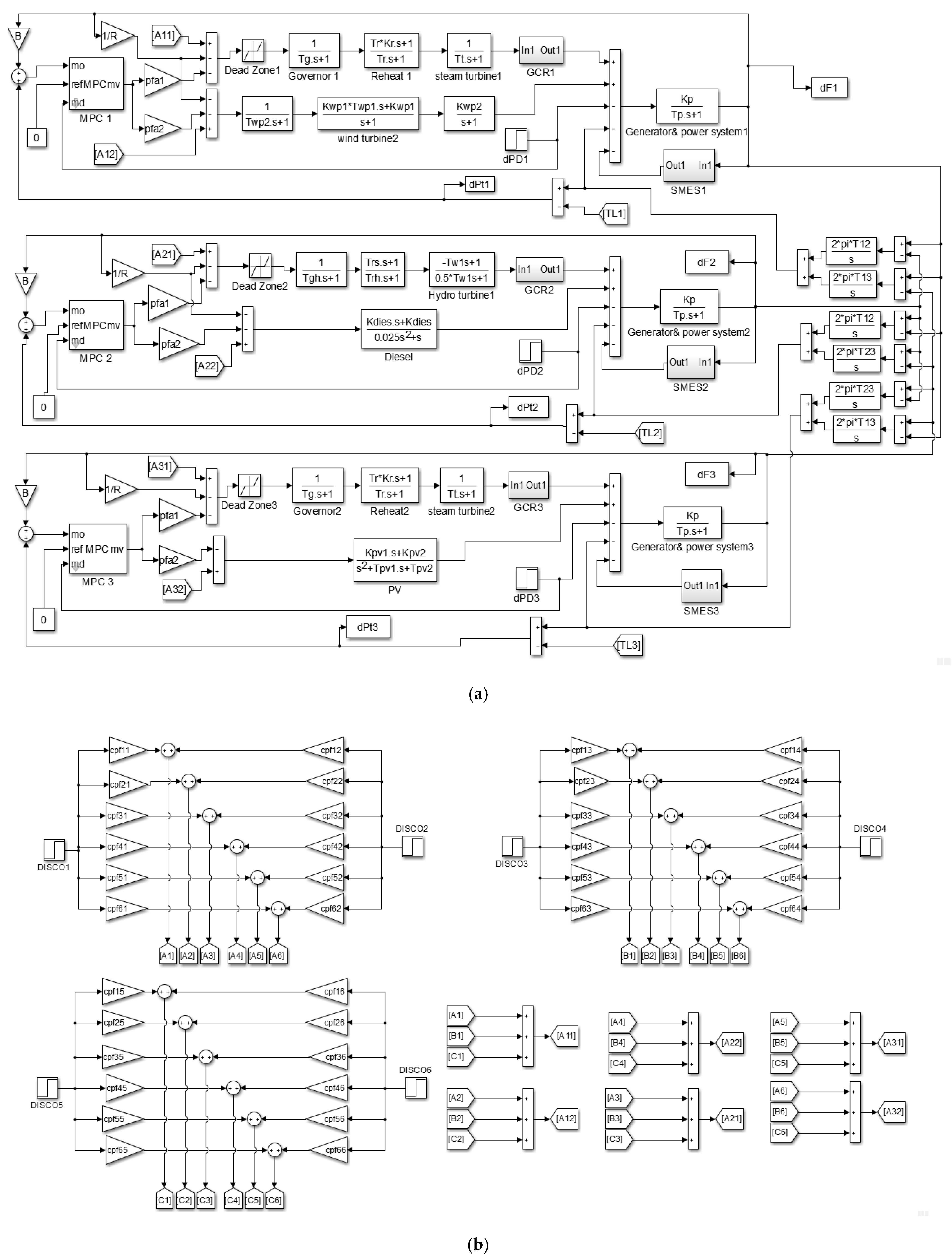
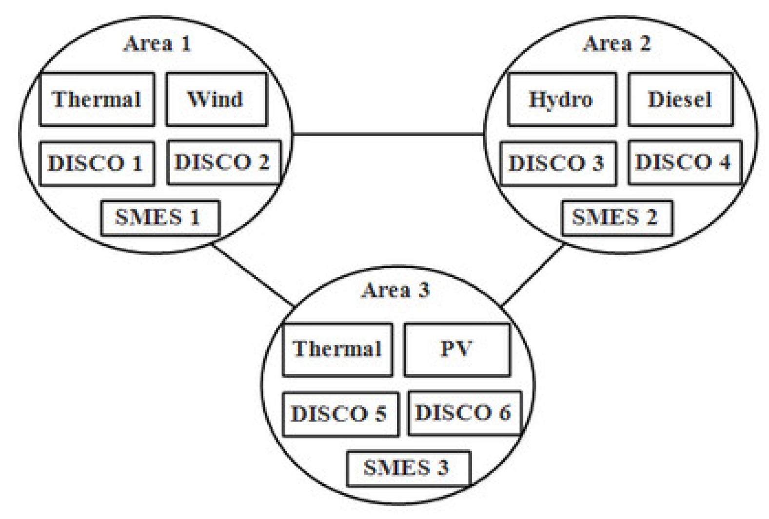
2. Mathematical Model of Deregulated LFC
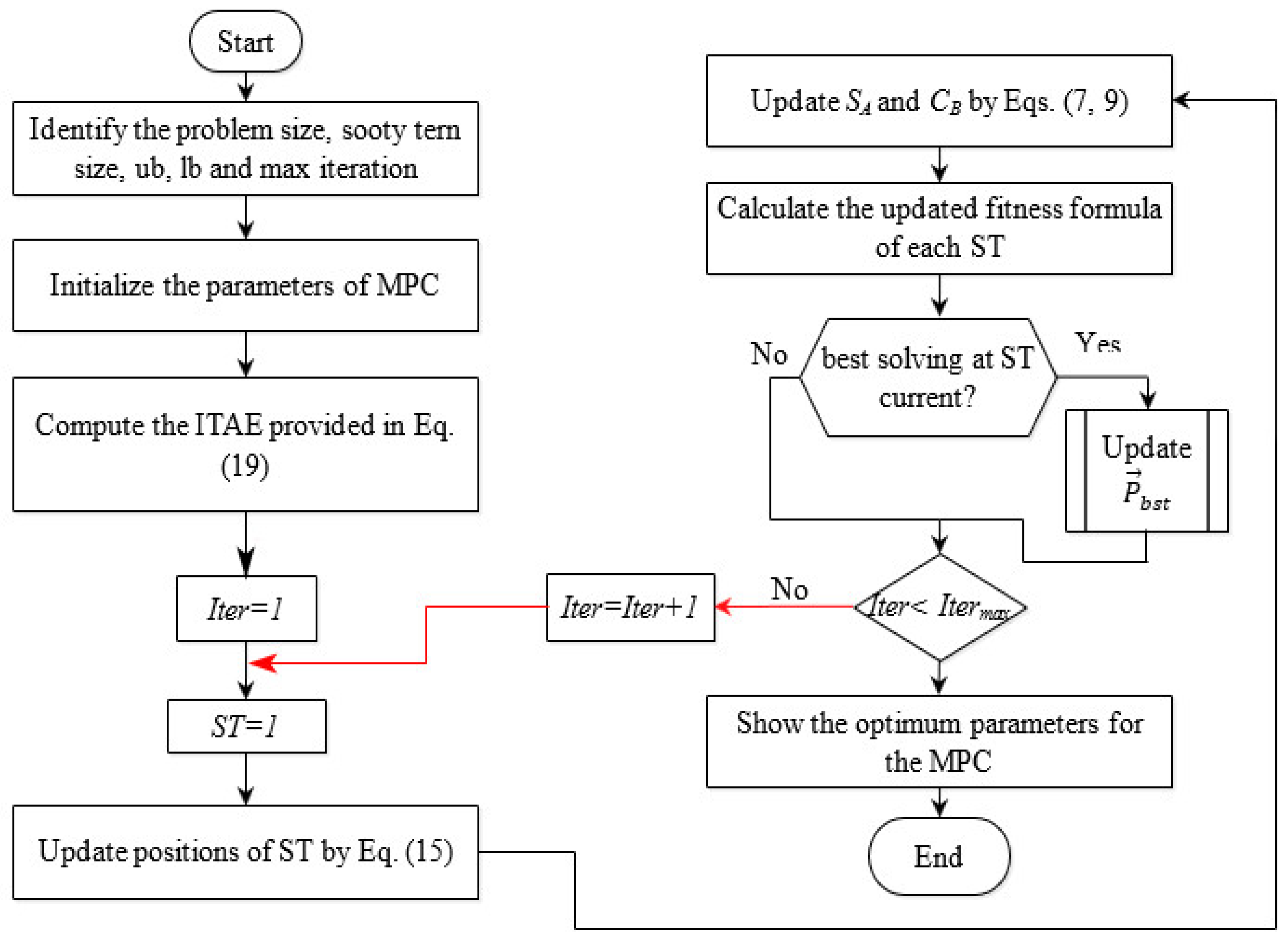
3. Sooty Terns Optimizer Characteristics
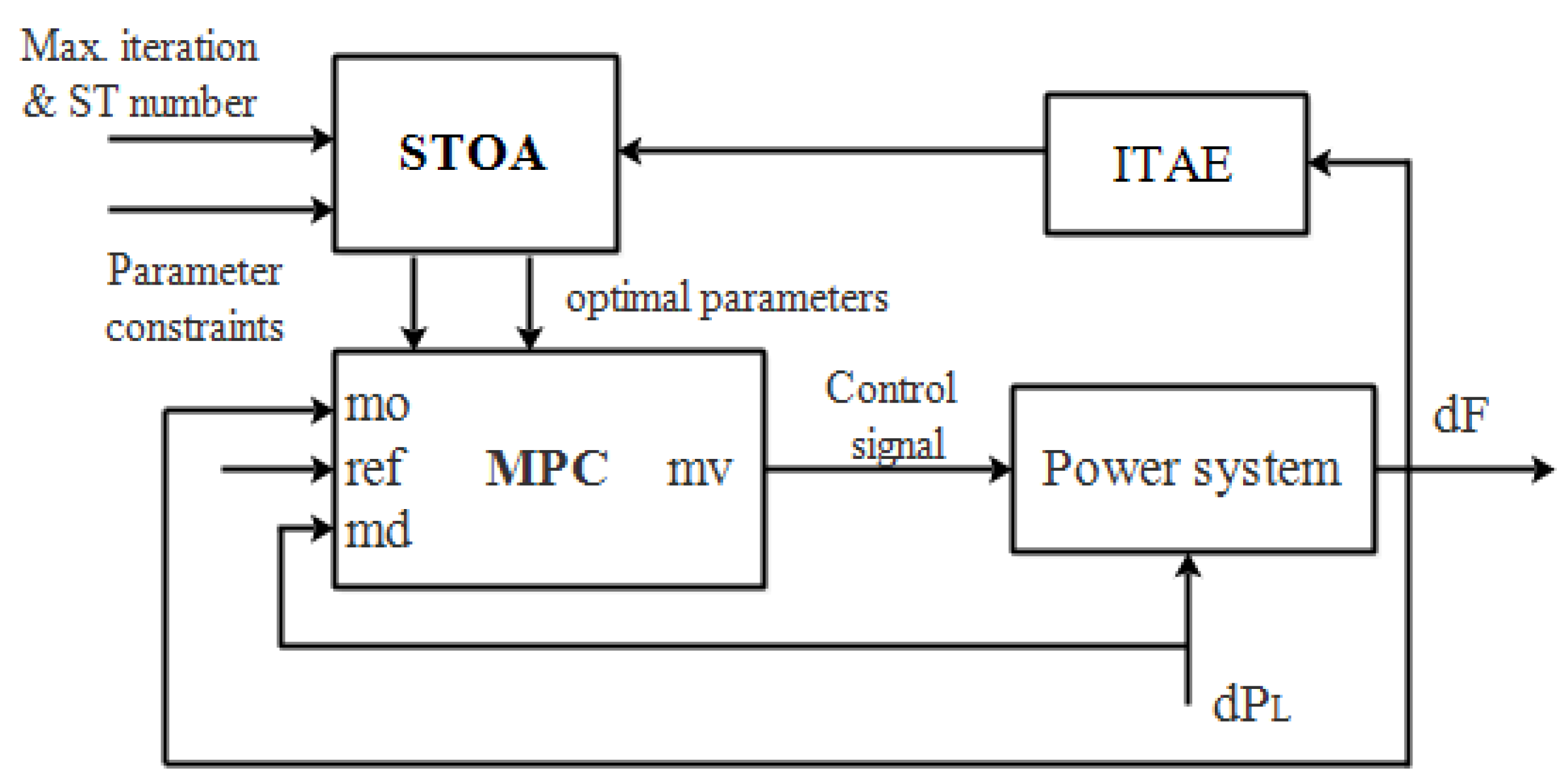
4. The Proposed Approach
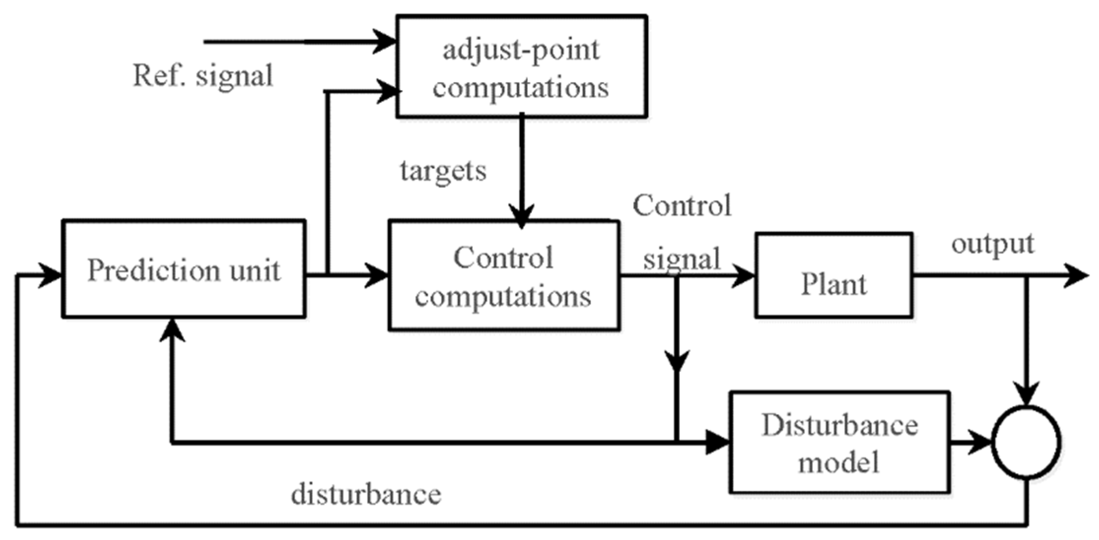
4.1. Model-Predictive Control (MPC)
4.2. Optimal Deregulated LFC Solving Problem
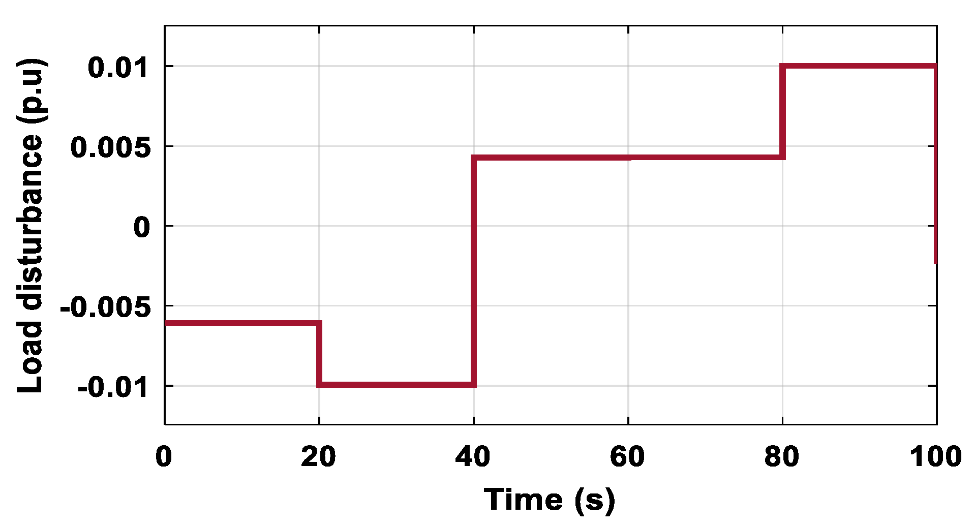
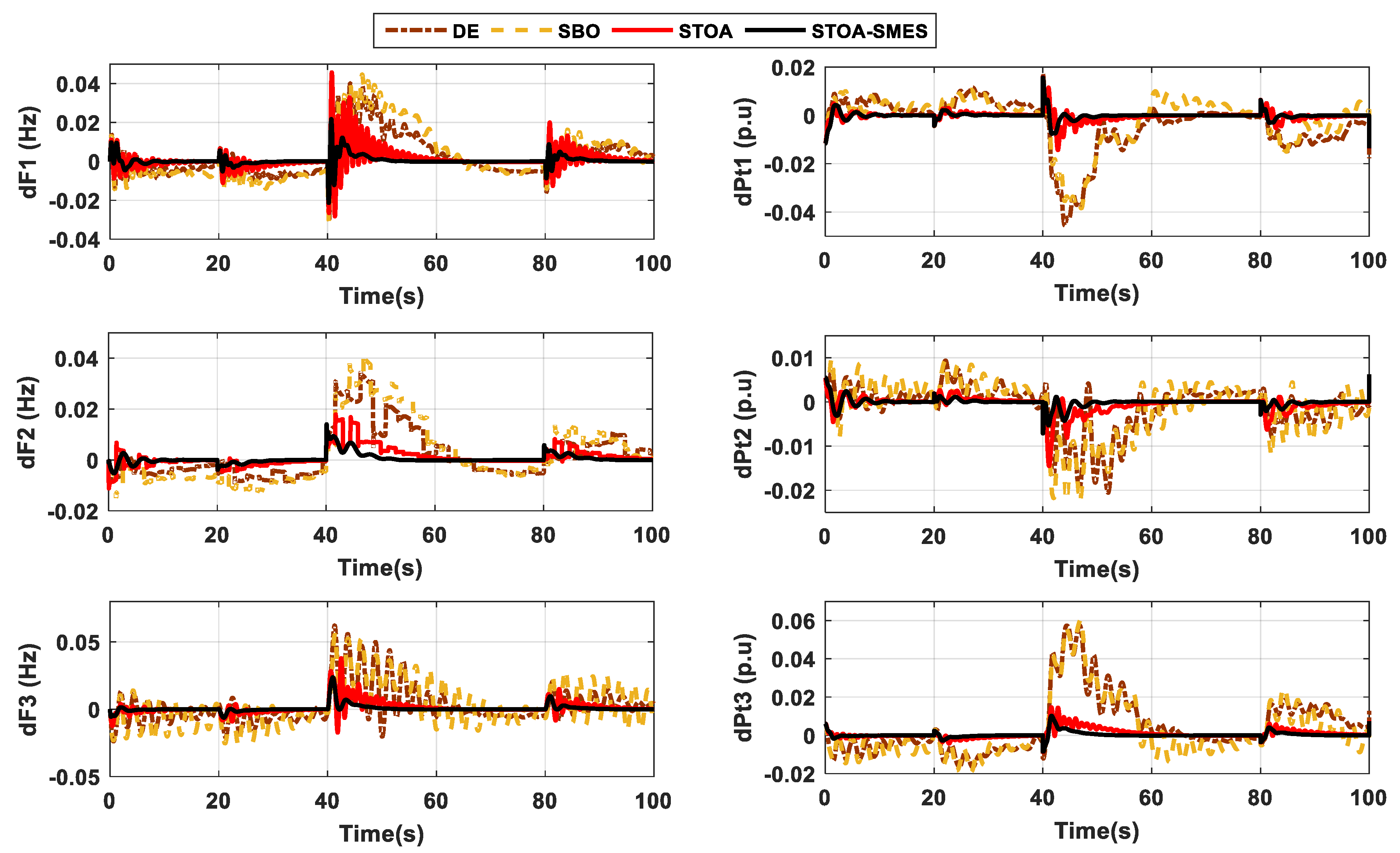
5. Simulation Results
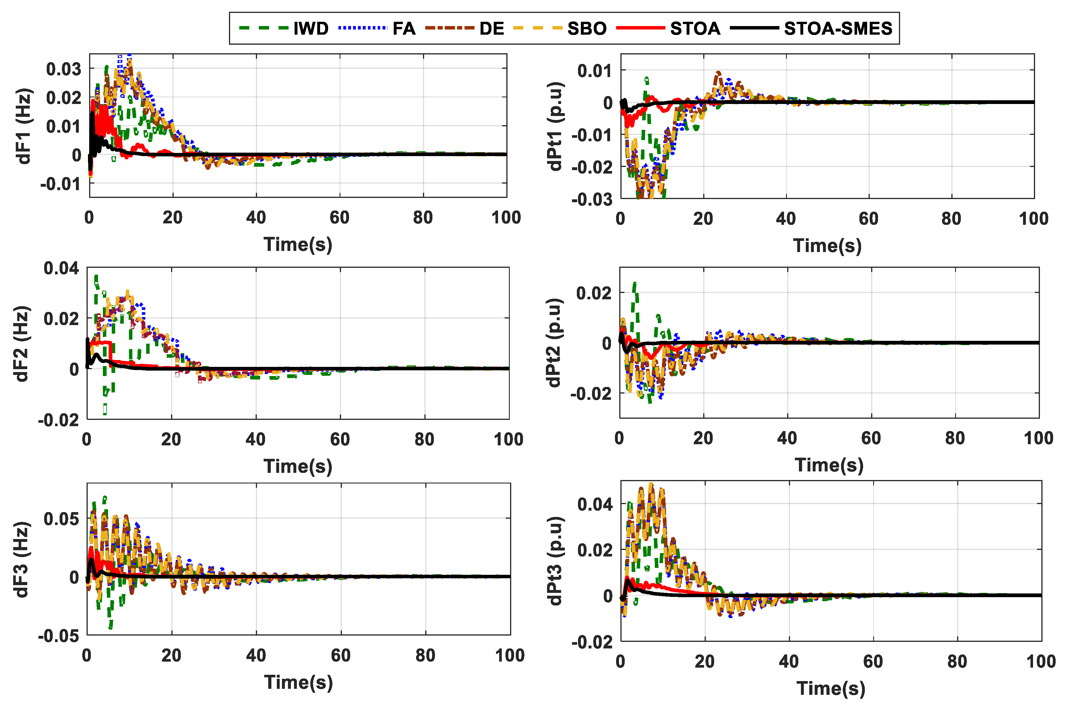
5.1. Unilateral-Based Transaction
5.2. Bilateral Transaction
5.3. Contract Violation Transaction
5.4. Sensitivity Analysis
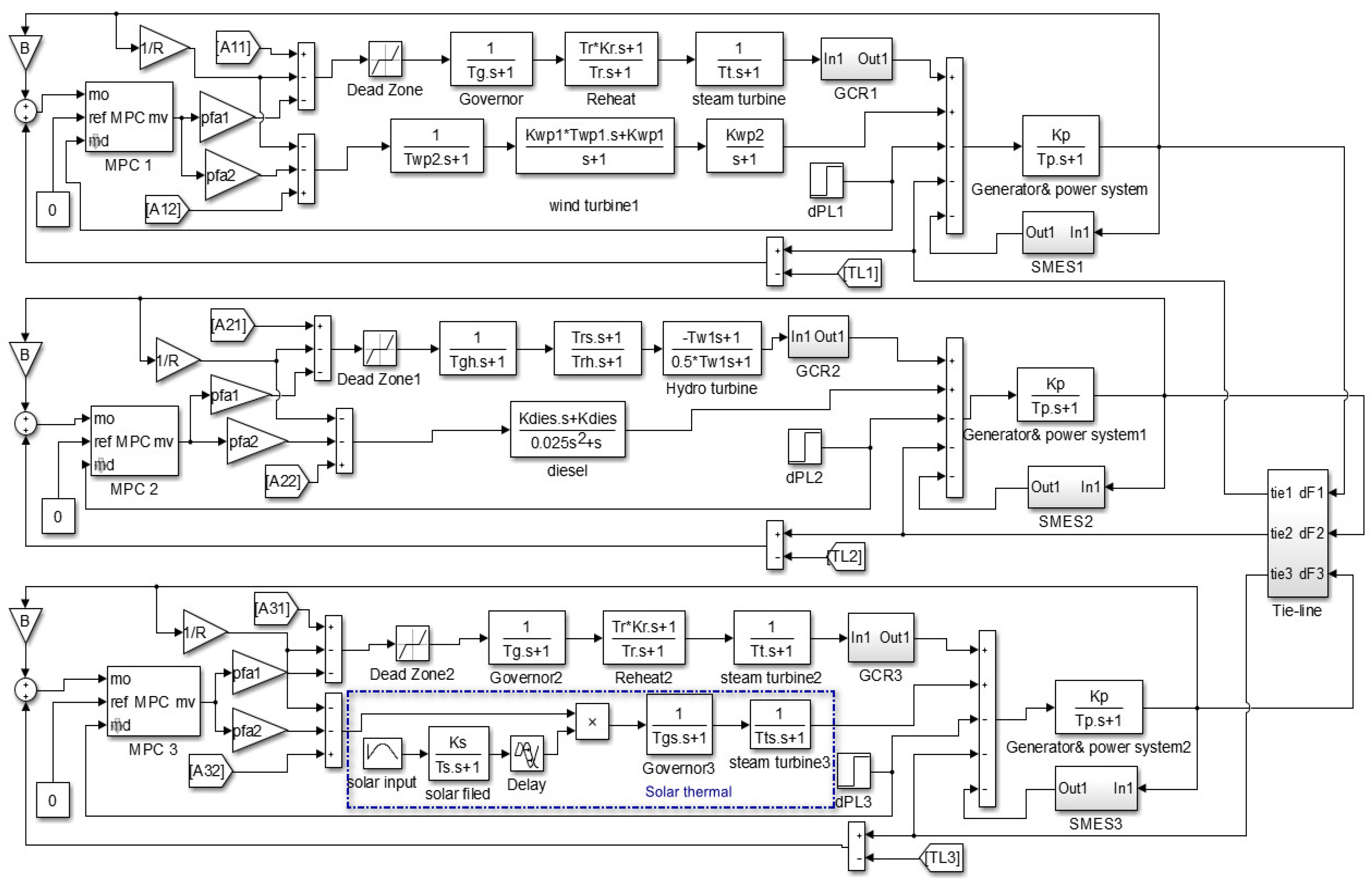
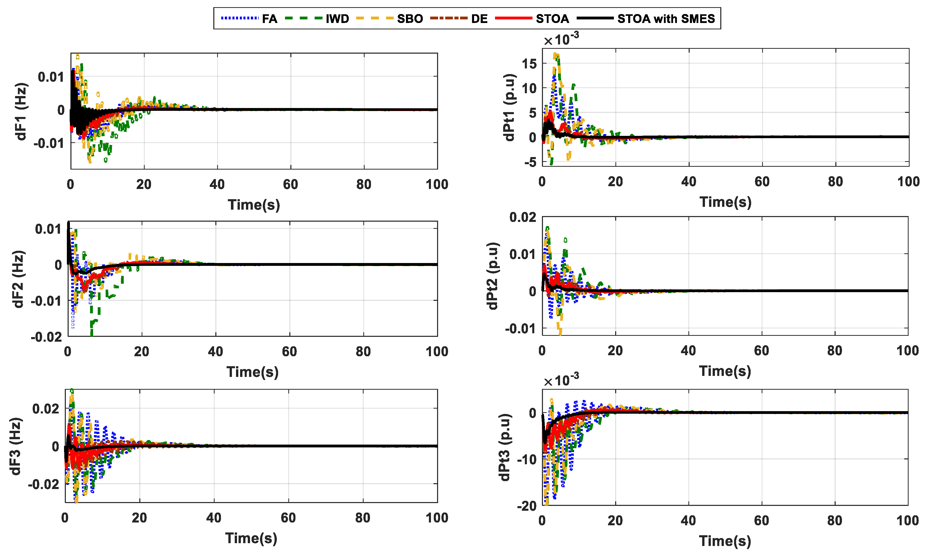
5.5. Practical Case Study
6. Conclusions
Author Contributions
Funding
Acknowledgments
Conflicts of Interest
Nomenclature
| STOA | Sooty terns optimization algorithm | ST | Sooty terns |
| LFC | Load frequency control | SBO | Stain bower braid algorithm |
| MPC | Model predictive control | FA | Firefly algorithm |
| TRANSCOs | Transmission companies | DE | Differential evolution |
| DISCOs | Distribution companies | PUs | Peak undershoot |
| GENCOs | Generation companies | POs | Peak overshoot |
| SMES | Superconducting magnetic energy storage | Ts | Settling time |
| DPM | DISCOs Participation Matrix | cpf | contract participation factor |
| Symbols | |||
| A, B, C and D | The system state space matrices | e | Normal logarithm |
| dPLi | The load disturbance in area i | Radi | The radius of every spiral turn |
| Tij | The coefficient of synchronizing between areas i and j | Rand | The random number in scale of [0, 1] |
| CB | The random variable | dPDi | total load disturbance in area i |
| The position of ST that does not conflict with ST another | x(k) | The system state | |
| Cf | Controlling variable | y(k) | The system outputs |
| The current position of sooty tern | z | The current iteration | |
| The ST positions of other | u and v | The constant of spiral form | |
| The disparity between the ST and excellent fittest ST | Kdies | The constant gain of diesel unit | |
| So and Si | the output and input diagonal array | Kg | The gain of steam plant governor |
| T | Sample time of MPC | Kgh | The gain of hydro plant governor |
| M and P | The control and prediction horizons | Kp | The gain of generator and power system |
| Q and R | Weighting factors | KPV1 and KPV2 | The gains of PV system |
| t | Simulation time | Kpw1, Kpw2 and Kpw3 | Wind plant gains |
| dFi | The frequency deviation of i area | Kr | The gain of reheater |
| dPtie,i | The power deviation of tie-line in area i | Kt | The gain of steam turbine |
| Tg | Time constant of governor (sec.) | Tr | Time constant of reheater (sec.) |
| Tgh | Time constant of hydro governor (sec.) | Trh | Reset time constants of hydro governor (sec.) |
| Tp | Time constant of generator and power system (sec.) | Trs | Hydro governor transient droop |
| TPV1 and TPV2 | Time constants of PV system (sec.) | Tt | Time constant of steam turbine (sec.) |
| Tpw1, Tpw2 and Tpw3 | Time constants of wind plant (sec.) | Tw | Nominal start time of the water in penstock (sec.) |
Appendix A

| Parameter | Value | Parameter | Value | Parameter | Value | |
|---|---|---|---|---|---|---|
| Tg | 0.08 s | Kpv1 | −18 | Kdiesel | 16.5 | |
| Tr | 10 s | Tpv1 | 100 s | R | 0.425 pu MW/Hz | |
| Kr | 0.33 Hz/pu MW | Kpv2 | 900 | B | 2.4 Hz/pu MW | |
| Tt | 0.3 s | Tpv2 | 50 s | apf1 | 0.65 | |
| Kp | 120 Hz/pu MW | Kwp1 | 1.25 | apf2 | 0.35 | |
| Tp | 20 s | Kwp2 | 1.4 | Twp1 | 6 s | |
| TW1 | 1 s | Twp2 | 0.041 s | Trs | 0.513 s | |
| Trh | 10 s | Tgh | 48.7 s | Ks | 1.8 | |
| Ts | 1.8 | Tgs | 1.0 | Tts | 3.0 | |
| Ksmes | T1 | T2 | T3 | T4 | Tsmes | |
| SMES1 | 0.8550 | 0.1279 | 0.1057 | 0.1000 | 0.6131 | 0.0144 |
| SMES2 | 0.8181 | 0.1377 | 0.5205 | 0.1030 | 0.4241 | 0.0849 |
| SMES3 | 0.5336 | 0.6088 | 0.1169 | 0.3597 | 0.2014 | 0.4638 |
References
- Veerasamy, V.; Member, S.; Izzri, N.; Wahab, A. A Hankel matrix based reduced order model for stability analysis of hybrid power system using PSO-GSA optimized cascade PI-PD controller for automatic load frequency control. IEEE Access 2020, 8, 71422–71446. [Google Scholar] [CrossRef]
- Arya, Y. AGC of restructured multi-area multi-source hydrothermal power systems incorporating energy storage units via optimal fractional-order fuzzy PID controller. Neural Comput. Appl. 2019, 31, 851–872. [Google Scholar] [CrossRef]
- Panwar, A.; Sharma, G.; Nasiruddin, I.; Bansal, R.C. Frequency stabilization of hydro–hydro power system using hybrid bacteria foraging PSO with UPFC and HAE. Electr. Power Syst. Res. 2018, 161, 74–85. [Google Scholar] [CrossRef]
- Pappachen, A.; Peer Fathima, A. Critical research areas on load frequency control issues in a deregulated power system: A state-of-the-art-of-review. Renew. Sustain. Energy Rev. 2017, 72, 163–177. [Google Scholar] [CrossRef]
- Haes Alhelou, H.; Hamedani-Golshan, M.E.; Zamani, R.; Heydarian-Forushani, E.; Siano, P. Challenges and opportunities of load frequency control in conventional, modern and future smart power systems: A comprehensive review. Energies 2018, 11, 2497. [Google Scholar] [CrossRef] [Green Version]
- Fathy, A.; Kassem, A.M.; Abdelaziz, A.Y. Optimal design of fuzzy PID controller for deregulated LFC of multi-area power system via mine blast algorithm. Neural Comput. Appl. 2020, 32, 4531–4551. [Google Scholar] [CrossRef]
- Tasnin, W.; Saikia, L.C. Impact of renewables and FACT device on deregulated thermal system having sine cosine algorithm optimised fractional order cascade controller. IET Renew. Power Gener. 2019, 13, 1420–1430. [Google Scholar] [CrossRef]
- Pappachen, A.; Peer Fathima, A. Load frequency control in deregulated power system integrated with SMES-TCPS combination using ANFIS controller. Int. J. Electr. Power Energy Syst. 2016, 82, 519–534. [Google Scholar] [CrossRef]
- Morsali, J.; Zare, K.; Tarafdar Hagh, M. A novel dynamic model and control approach for SSSC to contribute effectively in AGC of a deregulated power system. Int. J. Electr. Power Energy Syst. 2018, 95, 239–253. [Google Scholar] [CrossRef]
- Tasnin, W.; Saikia, L.C.; Raju, M. Deregulated AGC of multi-area system incorporating dish-Stirling solar thermal and geothermal power plants using fractional order cascade controller. Int. J. Electr. Power Energy Syst. 2018, 101, 60–74. [Google Scholar] [CrossRef]
- Khamari, D.; Sahu, R.K.; Gorripotu, T.S.; Panda, S. Automatic generation control of power system in deregulated environment using hybrid TLBO and pattern search technique. Ain Shams Eng. J. 2020, 11, 553–573. [Google Scholar] [CrossRef]
- Arya, Y.; Kumar, N. Design and analysis of BFOA-optimized fuzzy PI/PID controller for AGC of multi-area traditional/restructured electrical power systems. Soft Comput. 2017, 21, 6435–6452. [Google Scholar] [CrossRef]
- Mohanty, B. Hybrid flower pollination and pattern search algorithm optimized sliding mode controller for deregulated AGC system. J. Ambient Intell. Humaniz. Comput. 2020, 11, 763–776. [Google Scholar] [CrossRef]
- Kumari, S.; Shankar, G. Maiden application of cascade tilt-integral-derivative controller in load frequency control of deregulated power system. Int. Trans. Electr. Energy Syst. 2020, 30, e12257. [Google Scholar] [CrossRef]
- Nosratabadi, S.M.; Bornapour, M.; Gharaei, M.A. Grasshopper optimization algorithm for optimal load frequency control considering Predictive Functional Modified PID controller in restructured multi-resource multi-area power system with Redox Flow Battery units. Control Eng. Pract. 2019, 89, 204–227. [Google Scholar] [CrossRef]
- Prakash, A.; Murali, S.; Shankar, R.; Bhushan, R. HVDC tie-link modeling for restructured AGC using a novel fractional order cascade controller. Electr. Power Syst. Res. 2019, 170, 244–258. [Google Scholar] [CrossRef]
- Shiva, C.K.; Mukherjee, V. A novel quasi-oppositional harmony search algorithm for AGC optimization of three-area multi-unit power system after deregulation. Eng. Sci. Technol. Int. J. 2016, 19, 395–420. [Google Scholar] [CrossRef] [Green Version]
- Nandi, M.; Shiva, C.K.; Mukherjee, V. TCSC based automatic generation control of deregulated power system using quasi-oppositional harmony search algorithm. Eng. Sci. Technol. Int. J. 2017, 20, 1380–1395. [Google Scholar] [CrossRef]
- Shiva, C.K.; Mukherjee, V. Design and analysis of multi-source multi-area deregulated power system for automatic generation control using quasi-oppositional harmony search algorithm. Int. J. Electr. Power Energy Syst. 2016, 80, 382–395. [Google Scholar] [CrossRef]
- Mohanty, B.; Hota, P.K. Comparative performance analysis of fruit fly optimisation algorithm for multi-area multisource automatic generation control under deregulated environment. IET Gener. Transm. Distrib. 2015, 9, 1845–1855. [Google Scholar] [CrossRef]
- Prakash, A.; Kumar, K.; Parida, S.K. PIDF(1+FOD) controller for load frequency control with sssc and ac-dc tie-line in deregulated environment. IET Gener. Transm. Distrib. 2020, 14, 2751–2762. [Google Scholar] [CrossRef]
- Shankar, R.; Kumar, A.; Raj, U.; Chatterjee, K. Fruit fly algorithm-based automatic generation control of multiarea interconnected power system with FACTS and AC/DC links in deregulated power environment. Int. Trans. Electr. Energy Syst. 2019, 29, e2690. [Google Scholar] [CrossRef] [Green Version]
- Dhundhara, S.; Verma, Y.P. Capacitive energy storage with optimized controller for frequency regulation in realistic multisource deregulated power system. Energy 2018, 147, 1108–1128. [Google Scholar] [CrossRef]
- Ghasemi-marzbali, A. Multi-area multi-source automatic generation control in deregulated power system. Energy 2020, 201, 117667. [Google Scholar] [CrossRef]
- Selvaraju, R.K.; Somaskandan, G. Impact of energy storage units on load frequency control of deregulated power systems. Energy 2016, 97, 214–228. [Google Scholar] [CrossRef]
- Mishra, D.K.; Panigrahi, T.K.; Mohanty, A.; Ray, P.K. Effect of superconducting magnetic energy storage on two agent deregulated power system under open market. Mater. Today Proc. 2020, 21, 1919–1929. [Google Scholar] [CrossRef]
- Sharma, M.; Dhundhara, S.; Arya, Y.; Prakash, S. Frequency stabilization in deregulated energy system using coordinated operation of fuzzy controller and redox flow battery. Int. J. Energy Res. 2020, 45, 7457–7475. [Google Scholar] [CrossRef]
- Mishra, A.K.; Mishra, P.; Mathur, H.D. Enhancing the performance of a deregulated nonlinear integrated power system utilizing a redox flow battery with a self-tuning fractional-order fuzzy controller. ISA Trans. 2021. [Google Scholar] [CrossRef]
- Babu, N.R.; Saikia, L.C. Load frequency control of a multi-area system incorporating realistic high-voltage direct current and dish-Stirling solar thermal system models under deregulated scenario. IET Renew. Power Gener. 2021, 15, 1116–1132. [Google Scholar] [CrossRef]
- Kumar, R.; Sharma, V.K. Whale Optimization Controller for Load Frequency Control of a Two-Area Multi-source Deregulated Power System. Int. J. Fuzzy Syst. 2020, 22, 122–137. [Google Scholar] [CrossRef]
- Das, M.K.; Bera, P.; Sarkar, P.P. PID-RLNN controllers for discrete mode LFC of a three-area hydrothermal hybrid distributed generation deregulated power system. Int. Trans. Electr. Energy Syst. 2021, 31, 1–21. [Google Scholar] [CrossRef]
- Das, S.; Saikia, L.C.; Datta, S. Maiden application of TIDN-(1+PI) cascade controller in LFC of a multi-area hydro-thermal system incorporating EV–Archimedes wave energy-geothermal-wind generations under deregulated scenario. Int. Trans. Electr. Energy Syst. 2021, 31, e12907. [Google Scholar] [CrossRef]
- Raj, U.; Shankar, R. Deregulated Automatic Generation Control using Novel Opposition-based Interactive Search Algorithm Cascade Controller Including Distributed Generation and Electric Vehicle. Iran. J. Sci. Technol. Trans. Electr. Eng. 2020, 44, 1233–1251. [Google Scholar] [CrossRef]
- Kumar, A.; Shankar, R. A Quasi Opposition Lion Optimization Algorithm for Deregulated AGC Considering Hybrid Energy Storage System. J. Electr. Eng. Technol. 2021. [Google Scholar] [CrossRef]
- Dhiman, G.; Kaur, A. STOA: A bio-inspired based optimization algorithm for industrial engineering problems. Eng. Appl. Artif. Intell. 2019, 82, 148–174. [Google Scholar] [CrossRef]
- Seborg, D.E.; Edgar, T.F.; Mellichamp, D.A.; Doyle, F.J., III. Process Dynamics and Control, 4th ed.; Wiley: Seoul, Korea, 2017; ISBN 9781119298489. [Google Scholar]
- Mayne, D.Q. Model predictive control: Recent developments and future promise. Automatica 2014, 50, 2967–2986. [Google Scholar] [CrossRef]
- Elshafey, S.; Shehadeh, M.; Bayoumi, A.; Díaz, J.; Pernía, A.M.; Jose-Prieto, M.A.; Abdelmessih, G.Z. Solar thermal power in Egypt. In Proceedings of the 2018 IEEE Industry Applications Society Annual Meeting, IAS 2018, Portland, OR, USA, 23–27 September 2018; pp. 1–8. [Google Scholar] [CrossRef]
- Temraz, A.; Rashad, A.; Elweteedy, A.; Elshazly, K. Thermal Analysis of the Iscc Power Plant in Kuraymat, Egypt. Int. Conf. Appl. Mech. Mech. Eng. 2018, 18, 1–15. [Google Scholar] [CrossRef] [Green Version]


| Author | Year | Deregulated/ Conventional | Type of Controller | Optimization Approach | System Construction | Has RESs?/Type | Has ESs?/Type | Defects |
|---|---|---|---|---|---|---|---|---|
| Panwar, A. et al. [3] | 2018 | Conventional | PID | BFOA | 2 areas | √ (Fuel cell) | × |
|
| Shiva, C.K. et al. [17,18,19] | 2016–2017 | Deregulated | PID | QOHS | 2, 3 and 5 areas, multisources | × | × | |
| Mohanty, B. et al. [20] | 2015 | Deregulated | PIDD | FOA | 2-areas, multisources | × | × | |
| Dhundhara, S. et al. [23] | 2018 | Deregulated | PI | SCA | 2 areas, multisources | × | √ (CES) | |
| Ghasemi-marzbali, A. [24] | 2020 | Deregulated | PID | MVCS | 4 areas, multisources | × | × | |
| Selvaraju, R.K. et al. [25] | 2016 | Deregulated | PI | ACSA | 2 areas, multisources | × | √ (SMES and RFB) | |
| Kumar, R. et al. [30] | 2020 | Deregulated | PI | Wahle algorithm | 2 areas, multisources | × | √ (CES) | |
| Shankar, R. et al. [22] | 2019 | Deregulated | PID | FOA | 2 areas, multisources | × | × | |
| Kumar, A. et al. [34] | 2021 | Deregulated | PIDN | QOLOA | 2 areas, multisources | √ (WT and PV) | √ (SMES and RFB) | |
| Morsali, J. et al. [9] | 2018 | Deregulated | FOPID | MGSO | 2 areas, multisources | × | × |
|
| Prakash, A. et al. [21] | 2020 | Deregulated | PIDN(1+FOD) | SSA | 2 areas, multisources | √ (WT) | × | |
| Mishra, D.K. et al. [26] | 2020 | Deregulated | FOPID | Bat Algorithm | 2 areas, multisources | × | √ (SMES) | |
| Arya, Y. [2] | 2019 | Deregulated | FO-fuzzy PID | BFOA | 2 and 3 areas, multisources | × | √ (RFB) | |
| Mishra, A.K. et al. [28] | 2021 | Deregulated | FO-fuzzy PID | SSA | 3 areas, multisources | √ (WT, STPP and GTPP) | √ (RFB) | |
| Fathy, A. et al. [6] | 2020 | Conventional/deregulated | Fuzzy PID | MBA | 2 and 3 areas | × | × |
|
| Arya, Y. et al. [12] | 2017 | Conventional/deregulated | Fuzzy PI/PID | BFOA | 2 area/2 areas, multisources | × | × | |
| Sharma, M. et al. [27] | 2020 | Deregulated | Fuzzy PIDN | SSA | 2 areas, multisources | × | √ (RFB) | |
| Veerasamy, V. et al. [1] | 2020 | Conventional | Cascade PI-PD | PSO-GSA | 2 areas, multisources | √ (WT, Fuel cell) | √ (Battery) |
|
| Tasnin, W. et al. [7] | 2019 | Deregulated | Cascade FOI-FOPD | SCA | 3 areas, multisources | √ (WT, STPP and GTPP) | × | |
| Tasnin, W. et al. [10] | 2018 | Deregulated | Cascade FOPI-FOPID | SCA | 2 areas, multisources | √ (DSTS and GTPP) | × | |
| Kumari, S. et al. [14] | 2020 | Deregulated | Calculus-based cascade TI-TID | WCA | 4 areas, multisources | × | × | |
| Prakash, A. et al. [16] | 2019 | Deregulated | Cascade 2-DOF-PI-FOPDN | VPL | 2 areas, multisources | × | × | |
| Babu, N.R. et al. [29] | 2021 | Deregulated | Cascade FOPDN-FOPIDN | CA | 3 areas, multisources | √ (Realistic DSTS) | × | |
| Raj, U. et al. [33] | 2020 | Deregulated | Cascade 2DOF-PIDN-FOID | OISA | 3 areas, multisources | √ (WT and PV) | × | |
| Pappachen, A. et al. [8] | 2016 | Deregulated | ANFIS | × | 2 areas, multisources | × | √ (SMES) |
|
| Khamari, D. et al. [11] | 2020 | Deregulated | TID | hTLBO-PS | 2 areas, multisources | √ (Solar thermal) | √ (SMES) | |
| Mohanty, B. [13] | 2020 | Deregulated | Output feedback SMC | hFPA-PS | 2 areas, multisources | × | × | |
| Nosratabadi, S.M. et al. [15] | 2019 | Deregulated | Modified PID | GOA | 3 areas, multisources | √ (WT) | √ (RFB) | |
| Das, M.K. et al. [31] | 2021 | Deregulated | PID-RLNN | GOA | 3 areas, multisources | √ (WT) | √ (SMES) | |
| Das, S. et al. [32] | 2021 | Deregulated | TIDN-(1+PI) | MBA | 3 areas, multisources | √ (WT, GTPP and wave energy) | × | |
| Present study | Deregulated | Optimal MPC | STOA | 3 areas, multisources | √ (WT, PV and STPP) | √ (SMES) |
| Author | Year | Type of Controller | Optimization Approach | Linear/Nonlinear | Type of Generator | Has RESs?/Type | Cases Study | Has ESs?/Type | ||||
|---|---|---|---|---|---|---|---|---|---|---|---|---|
| 1 | 2 | 3 | 4 | 5 | ||||||||
| Arya, Y. [2] | 2019 | FO-fuzzy PID | BFOA | Linear | Thermal‒hydro | × | √ | √ | × | × | × | √ (RFB) |
| Tasnin, W. et al. [7] | 2019 | Cascade FOI-FOPD | SCA | Linear | Thermal | √ (WT, STPP and GTPP) | √ | √ | √ | × | × | × |
| Nosratabadi, S.M. et al. [15] | 2019 | Modified PID | GOA | Nonlinear (GRC-GDB) | Thermal‒hydro-gas‒diesel | √ (WT) | √ | √ | √ | √ | × | √ (RFB) |
| Shiva, C.K. et al. [17] | 2016 | PID | QOHS | Linear | Thermal | × | √ | √ | √ | × | × | × |
| Mishra, A.K. et al. [28] | 2021 | FO-fuzzy PID | SSA | Nonlinear (GRC-GDB) | Thermal | √ (WT, STPP and GTPP) | √ | √ | √ | √ | × | √ (RFB) |
| Babu, N.R. et al. [29] | 2021 | Cascade FOPDN-FOPIDN | CA | Nonlinear (GRC) | Thermal | √ (Realistic DSTS) | √ | √ | √ | × | × | × |
| Das, M.K. et al. [31] | 2021 | PID-RLNN | GOA | Linear | Thermal‒hydro‒diesel | √ (WT) | × | √ | √ | √ | × | √ (SMES) |
| Das, S. et al. [32] | 2021 | TIDN-(1 + PI) | MBA | Linear | Thermal‒hydro | √ (WT, GTPP and wave energy) | × | √ | × | × | × | × |
| Raj, U. et al. [33] | 2020 | Cascade 2DOF-PIDN-FOID | OISA | Linear | Thermal‒hydro‒gas‒diesel | √ (WT and PV) | √ | × | √ | × | × | × |
| Present study | Optimal MPC | STOA | Nonlinear (GRC-GDB) | Thermal‒hydro‒diesel | √ (WT, PV and STPP) | √ | √ | √ | √ | √ | √ (SMES) | |
| Algorithm | ITAE | IAE | ITSE | ISE |
|---|---|---|---|---|
| GOA [31] | 1.5881 | 0.1035 | 0.00064 | 0.00012 |
| IWD | 1.6434 | 0.1796 | 0.0022 | 0.0006 |
| FA | 1.5204 | 0.2097 | 0.0036 | 0.00099 |
| DE | 0.7078 | 0.1176 | 0.00096 | 0.00041 |
| SBO | 0.9502 | 0.1573 | 0.0020 | 0.00073 |
| STOA | 0.3736 | 0.0862 | 0.00057 | 0.00036 |
| STOA with SMES | 0.1302 | 0.0357 | 0.00011 | 0.00011 |
| Algorithm | Cont. | Parameter | ||||
|---|---|---|---|---|---|---|
| T | P | M | R | Q | ||
| IWD | MPC1 | 1.0188 | 4.0000 | 3.6313 | 8.0187 | 9.4088 |
| MPC2 | 1.4835 | 7.0000 | 3.0423 | 1.2121 | 4.1062 | |
| MPC3 | 1.7736 | 9.0000 | 2.3223 | 5.8237 | 2.5449 | |
| FA | MPC1 | 4.5778 | 7.0000 | 2.9508 | 7.1024 | 4.9171 |
| MPC2 | 7.9330 | 7.0000 | 2.8788 | 6.8717 | 2.1063 | |
| MPC3 | 4.1919 | 7.0000 | 2.5025 | 6.3966 | 6.1616 | |
| DE | MPC1 | 0.1058 | 10.000 | 1.0000 | 9.5576 | 1.8960 |
| MPC2 | 0.1714 | 10.000 | 1.0316 | 1.0000 | 9.9312 | |
| MPC3 | 8.0646 | 4.0000 | 1.0000 | 9.7133 | 7.2729 | |
| SBO | MPC1 | 2.2503 | 7.0000 | 3.4737 | 4.2343 | 8.6914 |
| MPC2 | 7.2548 | 7.0000 | 2.0266 | 7.2507 | 1.9411 | |
| MPC3 | 6.6740 | 8.0000 | 3.2194 | 8.8556 | 9.1734 | |
| STOA | MPC1 | 0.1015 | 10.000 | 1.6962 | 1.0000 | 4.7993 |
| MPC2 | 0.1425 | 5.0000 | 1.0000 | 1.0098 | 10.000 | |
| MPC3 | 0.1000 | 5.0000 | 2.1788 | 1.0037 | 10.000 | |
| STOA with SMES | MPC1 | 0.9897 | 6.0000 | 3.0211 | 1.0000 | 10.000 |
| MPC2 | 0.1114 | 9.0000 | 1.0329 | 1.0000 | 3.6893 | |
| MPC3 | 0.1163 | 7.0000 | 3.7377 | 9.3049 | 1.0792 | |
| Sig. | MPC via IWD | MPC via FA | MPC via DE | ||||||
|---|---|---|---|---|---|---|---|---|---|
| Ts (s) | PUs (Hz) | Pos (Hz) | Ts (s) | PUs (Hz) | Pos (Hz) | Ts (s) | PUs (Hz) | Pos (Hz) | |
| dF1 | 27.0376 | −0.0086 | 0.0168 | 19.0569 | −0.0067 | 0.0179 | 14.6580 | −0.0066 | 0.0164 |
| dF2 | 31.1874 | −0.0056 | 0.0052 | 31.7522 | −0.0004 | 0.0007 | 20.7756 | −0.0019 | 0.0066 |
| dF3 | 33.0361 | −0.0048 | 0.0080 | 32.3542 | −0.0058 | 0.0090 | 26.9215 | −0.0039 | 0.0081 |
| dPtie1 | 25.2028 | −0.0048 | 0.0062 | 25.3927 | −0.0016 | 0.0102 | 21.6732 | −0.0029 | 0.0061 |
| dPtie2 | 28.6876 | −0.0049 | 0.0033 | 26.9591 | −0.0092 | 0.0018 | 22.6277 | −0.0047 | 0.0023 |
| dPtie3 | 49.6124 | −0.0032 | 0.0024 | 35.4933 | −0.0034 | 0.0021 | 31.1791 | −0.0031 | 0.0015 |
| MPC via SBO | MPC via STOA | MPC via STOA with SMES | |||||||
| dF1 | 19.7260 | −0.0075 | 0.0187 | 10.0692 | −0.0064 | 0.0178 | 10.9544 | −0.0055 | 0.0133 |
| dF2 | 29.1531 | −0.0004 | 0.0007 | 15.7320 | −0.0020 | 0.0053 | 7.8413 | −0.0003 | 0.0022 |
| dF3 | 28.6542 | −0.0062 | 0.0093 | 11.3257 | −0.0078 | 0.0119 | 10.3924 | −0.0006 | 0.0024 |
| dPtie1 | 21.2646 | −0.0016 | 0.0083 | 10.9328 | −0.0028 | 0.0069 | 10.2124 | −0.0012 | 0.0045 |
| dPtie2 | 20.5120 | −0.0097 | 0.0010 | 10.9060 | −0.0046 | 0.0026 | 9.3023 | −0.0024 | 0.0006 |
| dPtie3 | 33.0939 | −0.0035 | 0.0022 | 10.7960 | −0.0032 | 0.0022 | 10.2997 | −0.0021 | 0.0006 |
| Algorithm | ITAE | IAE | ITSE | ISE |
|---|---|---|---|---|
| IWD | 35.6750 | 2.1620 | 0.2921 | 0.0385 |
| FA | 33.2202 | 2.4408 | 0.4506 | 0.0499 |
| DE | 30.1369 | 2.3571 | 0.4204 | 0.0493 |
| SBO | 32.1007 | 2.3821 | 0.4301 | 0.0487 |
| STOA | 3.2369 | 0.3996 | 0.0102 | 0.0028 |
| STOA with SMES | 0.6619 | 0.1343 | 0.0011 | 0.00055 |
| Algorithm | Cont. | Parameter | ||||
|---|---|---|---|---|---|---|
| T | P | M | R | Q | ||
| IWD | MPC1 | 6.1667 | 8.0000 | 3.7863 | 8.2602 | 6.2492 |
| MPC2 | 2.0503 | 5.0000 | 3.8281 | 1.4377 | 5.5301 | |
| MPC3 | 1.8900 | 10.000 | 3.5589 | 5.8544 | 5.7842 | |
| FA | MPC1 | 6.8705 | 6.0000 | 2.5811 | 6.4681 | 3.3892 |
| MPC2 | 2.3363 | 7.0000 | 2.5216 | 5.2274 | 5.8524 | |
| MPC3 | 9.3026 | 8.0000 | 1.6665 | 7.1737 | 4.7571 | |
| DE | MPC1 | 2.5035 | 4.0000 | 2.2353 | 7.0311 | 1.8310 |
| MPC2 | 2.6587 | 6.0000 | 3.6384 | 2.6987 | 9.4498 | |
| MPC3 | 9.4381 | 4.0000 | 1.6674 | 10.000 | 6.0715 | |
| SBO | MPC1 | 2.9720 | 7.0000 | 1.2831 | 9.6783 | 2.6398 |
| MPC2 | 1.1842 | 6.0000 | 1.6785 | 4.3008 | 4.5068 | |
| MPC3 | 9.3530 | 10.000 | 1.1492 | 6.9536 | 5.1313 | |
| STOA | MPC1 | 0.3460 | 10.000 | 3.1737 | 1.0000 | 1.1277 |
| MPC2 | 5.4724 | 6.0000 | 3.3661 | 1.0000 | 7.1087 | |
| MPC3 | 0.1000 | 4.2887 | 4.0000 | 1.0000 | 10.000 | |
| STOA with SMES | MPC1 | 0.1068 | 4.0000 | 3.1802 | 1.2149 | 7.1680 |
| MPC2 | 0.1051 | 4.0000 | 1.8494 | 1.1014 | 7.6772 | |
| MPC3 | 0.1000 | 5.0000 | 3.2439 | 1.0000 | 10.000 | |
| Sig. | MPC via IWD | MPC via FA | MPC via DE | ||||||
|---|---|---|---|---|---|---|---|---|---|
| Ts (s) | PUs (Hz) | Pos (Hz) | Ts (s) | PUs (Hz) | Pos (Hz) | Ts (s) | PUs (Hz) | Pos (Hz) | |
| dF1 | 63.9004 | −0.0072 | 0.0306 | 53.6476 | −0.0074 | 0.0349 | 43.7017 | −0.0078 | 0.0319 |
| dF2 | 63.5724 | −0.0199 | 0.0376 | 53.3038 | 0.0026 | 0.028 | 45.2208 | −0.0057 | 0.0284 |
| dF3 | 60.1116 | −0.0442 | 0.0680 | 56.1535 | −0.0142 | 0.0566 | 52.0592 | −0.0143 | 0.0558 |
| dPtie1 | 68.2425 | −0.0306 | 0.0075 | 45.1001 | −0.0292 | 0.0070 | 42.9730 | −0.0317 | 0.0092 |
| dPtie2 | 61.5340 | −0.0246 | 0.0236 | 54.0869 | −0.0219 | 0.0048 | 51.4809 | −0.0189 | 0.0042 |
| dPtie3 | 54.8649 | −0.0039 | 0.0463 | 49.0363 | −0.0092 | 0.0469 | 46.4990 | −0.0085 | 0.0480 |
| MPC via SBO | MPC via STOA | MPC via STOA with SMES | |||||||
| dF1 | 50.5606 | −0.0077 | 0.0328 | 21.8899 | −0.0069 | 0.0187 | 11.4348 | −0.0053 | 0.0146 |
| dF2 | 49.7371 | −0.0046 | 0.0315 | 41.6452 | −0.0004 | 0.0105 | 10.6745 | −0.0001 | 0.0117 |
| dF3 | 55.3097 | −0.0188 | 0.0553 | 18.4991 | −0.0048 | 0.0242 | 9.9298 | −0.0044 | 0.0146 |
| dPtie1 | 42.3331 | −0.0306 | 0.0061 | 24.2308 | −0.0076 | 0.0016 | 14.1611 | −0.0030 | 0.0007 |
| dPtie2 | 51.1851 | −0.0211 | 0.0044 | 46.4254 | −0.0062 | 0.0023 | 9.5737 | −0.0037 | 7.3 × 10⁻⁵ |
| dPtie3 | 45.8561 | −0.0089 | 0.0487 | 41.7109 | −0.0002 | 0.0078 | 11.7334 | −9.9 × 10⁻⁵ | 0.0066 |
| Algorithm | ITAE | IAE | ITSE | ISE |
|---|---|---|---|---|
| IWD | 53.9881 | 3.1885 | 0.6218 | 0.0785 |
| FA | 49.0131 | 3.7460 | 1.1571 | 0.1293 |
| DE | 46.3893 | 3.6482 | 1.0186 | 0.1222 |
| SBO | 47.0683 | 3.5857 | 1.0208 | 0.1184 |
| STOA | 5.1892 | 0.6027 | 0.0210 | 0.0056 |
| STOA with SMES | 1.0106 | 0.2071 | 0.0025 | 0.0012 |
| Algorithm | Cont. | Parameter | ||||
|---|---|---|---|---|---|---|
| T | P | M | R | Q | ||
| IWD | MPC1 | 6.1667 | 8.0000 | 3.7863 | 8.2602 | 6.2492 |
| MPC2 | 2.0503 | 5.0000 | 3.8281 | 1.4377 | 5.5301 | |
| MPC3 | 1.8900 | 10.000 | 3.5589 | 5.8544 | 5.7842 | |
| FA | MPC1 | 5.2872 | 6.0000 | 2.9868 | 6.3122 | 4.0850 |
| MPC2 | 1.2944 | 8.0000 | 1.7920 | 5.3635 | 6.3384 | |
| MPC3 | 9.3368 | 9.0000 | 1.5967 | 4.5315 | 3.9342 | |
| DE | MPC1 | 10.000 | 6.0000 | 1.0000 | 10.000 | 4.1331 |
| MPC2 | 2.3147 | 9.0000 | 2.3905 | 1.0000 | 3.4827 | |
| MPC3 | 9.2692 | 10.000 | 1.3768 | 7.5380 | 8.5526 | |
| SBO | MPC1 | 2.8428 | 7.0000 | 1.0952 | 9.8400 | 2.6615 |
| MPC2 | 1.3013 | 6.0000 | 1.6362 | 3.7066 | 5.3726 | |
| MPC3 | 9.3763 | 10.000 | 1.3055 | 7.5704 | 3.4958 | |
| STOA | MPC1 | 0.3863 | 6.0000 | 1.3697 | 1.0000 | 10.000 |
| MPC2 | 1.3889 | 10.000 | 1.7762 | 1.0000 | 10.000 | |
| MPC3 | 0.1000 | 4.0000 | 4.0000 | 1.0000 | 10.000 | |
| STOA with SMES | MPC1 | 0.1061 | 8.0000 | 1.1080 | 1.1258 | 8.9523 |
| MPC2 | 0.1092 | 4.0000 | 1.2645 | 2.1158 | 8.0565 | |
| MPC3 | 0.1000 | 7.0000 | 2.4561 | 1.0000 | 10.000 | |
| Sig. | MPC via IWD | MPC via FA | MPC via DE | ||||||
|---|---|---|---|---|---|---|---|---|---|
| Ts (s) | PUs (Hz) | Pos (Hz) | Ts (s) | PUs (Hz) | Pos (Hz) | Ts (s) | PUs (Hz) | Pos (Hz) | |
| dF1 | 63.9340 | −0.0165 | 0.0454 | 47.9268 | −0.0166 | 0.0557 | 51.4054 | −0.0167 | 0.0507 |
| dF2 | 63.5803 | −0.0238 | 0.0497 | 49.1896 | −0.0074 | 0.0511 | 53.2465 | −0.0033 | 0.0450 |
| dF3 | 60.3591 | −0.0558 | 0.0901 | 55.4846 | −0.0242 | 0.0882 | 53.9884 | −0.0259 | 0.0826 |
| dPtie1 | 68.2835 | −0.0448 | 0.0054 | 47.3875 | −0.0447 | 0.0081 | 47.4371 | −0.0558 | 0.0080 |
| dPtie2 | 61.5780 | −0.0344 | 0.0305 | 53.6804 | −0.0333 | 0.0107 | 54.8810 | −0.0256 | 0.0115 |
| dPtie3 | 55.0195 | −0.0047 | 0.0649 | 48.6736 | −0.0102 | 0.0747 | 49.5926 | −0.0066 | 0.0706 |
| MPC via SBO | MPC via STOA | MPC via STOA with SMES | |||||||
| dF1 | 53.5217 | −0.0168 | 0.0516 | 20.5473 | −0.0142 | 0.0331 | 11.4963 | −0.0125 | 0.0176 |
| dF2 | 56.2937 | −0.0047 | 0.0450 | 37.5205 | −0.0004 | 0.0203 | 11.8392 | −0.0002 | 0.0170 |
| dF3 | 53.2066 | −0.0240 | 0.0817 | 19.9847 | −0.0073 | 0.0388 | 10.6878 | −0.0040 | 0.0214 |
| dPtie1 | 42.3381 | −0.0482 | 0.0058 | 22.3325 | −0.0124 | 0.0003 | 12.8129 | −0.0059 | 0.0005 |
| dPtie2 | 53.7500 | −0.0287 | 0.0120 | 35.5661 | −0.0088 | 0.0063 | 21.0063 | −0.0042 | 0.0041 |
| dPtie3 | 46.4073 | −0.0083 | 0.0751 | 41.1126 | −0.0003 | 0.0122 | 11.7787 | −0.0002 | 0.0099 |
| Parameter | Bilateral Transaction | Contract Violation | ||||||
|---|---|---|---|---|---|---|---|---|
| ITAE (0.6619) | ITAE (1.0106) | |||||||
| −50% | −25% | +25% | +50% | −50% | −25% | +25% | +50% | |
| Tg | 0.6619 | 0.6619 | 0.6619 | 0.6618 | 1.0106 | 1.0106 | 1.0106 | 1.0106 |
| Kr | 0.6619 | 0.6619 | 0.6619 | 0.6618 | 1.0106 | 1.0106 | 1.0106 | 1.0106 |
| Tr | 0.6619 | 0.6619 | 0.6619 | 0.6618 | 1.0106 | 1.0106 | 1.0106 | 1.0106 |
| Tt | 0.6619 | 0.6619 | 0.6619 | 0.6618 | 1.0106 | 1.0106 | 1.0106 | 1.0106 |
| Kp | 0.7049 | 0.6651 | 0.6607 | 0.6606 | 1.1089 | 1.0157 | 1.0094 | 1.0090 |
| Tp | 0.6826 | 0.6606 | 0.6640 | 0.6678 | 1.0105 | 1.0094 | 1.0137 | 1.0195 |
| Algorithm | ITAE | IAE | ITSE | ISE |
|---|---|---|---|---|
| IWD | 8.1699 | 0.7598 | 0.0419 | 0.0074 |
| FA | 5.7623 | 0.5724 | 0.0253 | 0.0052 |
| DE | 2.7636 | 0.2837 | 0.0054 | 0.0012 |
| SBO | 6.0784 | 0.5965 | 0.0230 | 0.0055 |
| STOA | 1.9642 | 0.2347 | 0.0036 | 9.74 × 10⁻⁴ |
| STOA with SMES | 0.7647 | 0.1092 | 6.65 × 10⁻⁴ | 3.03 × 10⁻⁴ |
| Algorithm | Cont. | Parameter | ||||
|---|---|---|---|---|---|---|
| T | P | M | R | Q | ||
| IWD | MPC1 | 2.2386 | 6.0000 | 2.7958 | 3.1128 | 8.6028 |
| MPC2 | 2.0960 | 5.0000 | 1.7696 | 3.0907 | 5.4609 | |
| MPC3 | 3.2193 | 10.000 | 2.8946 | 2.7096 | 9.1469 | |
| FA | MPC1 | 2.3419 | 5.0000 | 2.5255 | 3.8603 | 7.9511 |
| MPC2 | 1.1804 | 5.0000 | 1.6602 | 2.6835 | 5.7731 | |
| MPC3 | 2.6442 | 9.0000 | 2.1220 | 2.1650 | 9.2610 | |
| DE | MPC1 | 0.1000 | 7.0000 | 2.6028 | 1.1892 | 9.7307 |
| MPC2 | 0.1003 | 8.0000 | 1.0000 | 1.0010 | 9.8950 | |
| MPC3 | 0.1000 | 10.000 | 4.0000 | 1.0007 | 9.9993 | |
| SBO | MPC1 | 2.2841 | 6.0000 | 2.5856 | 3.1844 | 8.4974 |
| MPC2 | 1.8531 | 6.0000 | 1.6108 | 3.1598 | 5.2159 | |
| MPC3 | 3.03711 | 9.0000 | 2.3412 | 1.0113 | 9.2644 | |
| STOA | MPC1 | 0.1306 | 6.0000 | 1.1957 | 1.6546 | 4.2269 |
| MPC2 | 0.1072 | 10.000 | 1.4580 | 1.2117 | 4.0086 | |
| MPC3 | 0.1000 | 4.0000 | 1.2055 | 1.0000 | 10.0000 | |
| STOA with SMES | MPC1 | 0.1000 | 5.0000 | 3.2188 | 1.0000 | 10.000 |
| MPC2 | 0.1000 | 10.000 | 1.9825 | 1.0000 | 8.5687 | |
| MPC3 | 0.1000 | 5.0000 | 1.1332 | 1.0000 | 10.000 | |
| Sig. | MPC via IWD | MPC via FA | MPC via DE | ||||||
|---|---|---|---|---|---|---|---|---|---|
| Ts (s) | PUs (Hz) | Pos (Hz) | Ts (s) | PUs (Hz) | Pos (Hz) | Ts (s) | PUs (Hz) | Pos (Hz) | |
| dF1 | 38.2310 | −0.0157 | 0.0163 | 35.5070 | −0.0091 | 0.0124 | 29.0191 | −0.0079 | 0.0098 |
| dF2 | 33.5896 | −0.0207 | 0.0106 | 33.0856 | −0.0178 | 0.0106 | 28.0973 | −0.0078 | 0.0117 |
| dF3 | 34.2854 | −0.0273 | 0.0300 | 33.3888 | −0.0297 | 0.0240 | 38.2454 | −0.0132 | 0.0118 |
| dPtie1 | 32.4268 | −0.0055 | 0.0172 | 31.6296 | −0.0011 | 0.0126 | 30.9189 | −0.0007 | 0.0047 |
| dPtie2 | 30.0549 | −0.0077 | 0.0141 | 29.4559 | −0.0075 | 0.0089 | 30.1285 | −0.0014 | 0.0051 |
| dPtie3 | 34.7497 | −0.0174 | 0.0020 | 31.8582 | −0.0187 | 0.0026 | 30.9790 | −0.0017 | 0.0011 |
| MPC via SBO | MPC via STOA | MPC via STOA with SMES | |||||||
| dF1 | 35.4207 | −0.016 | 0.0165 | 25.3660 | −0.0087 | 0.0117 | 15.3465 | −0.0073 | 0.0115 |
| dF2 | 35.2094 | −0.0132 | 0.0106 | 25.7349 | −0.0068 | 0.0115 | 14.3275 | −0.0027 | 0.0115 |
| dF3 | 32.4255 | −0.0308 | 0.0287 | 26.5229 | −0.0118 | 0.0103 | 14.9977 | −0.0082 | 0.0054 |
| dPtie1 | 30.6435 | −0.0053 | 0.0170 | 27.0556 | −0.0012 | 0.0051 | 20.9348 | −0.0006 | 0.0034 |
| dPtie2 | 32.5795 | −0.0121 | 0.0073 | 22.5349 | −0.0004 | 0.0045 | 13.8070 | −1.6 × 10⁻⁶ | 9.4805 |
| dPtie3 | 32.9513 | −0.0173 | 0.0029 | 27.0283 | −0.0005 | 0.0006 | 11.7035 | −4.5 × 10⁻⁵ | 5.6 × 10⁻⁵ |
Publisher’s Note: MDPI stays neutral with regard to jurisdictional claims in published maps and institutional affiliations. |
© 2021 by the authors. Licensee MDPI, Basel, Switzerland. This article is an open access article distributed under the terms and conditions of the Creative Commons Attribution (CC BY) license (https://creativecommons.org/licenses/by/4.0/).
Share and Cite
Ali, H.H.; Fathy, A.; Al-Shaalan, A.M.; Kassem, A.M.; M. H. Farh, H.; Al-Shamma’a, A.A.; A. Gabbar, H. A Novel Sooty Terns Algorithm for Deregulated MPC-LFC Installed in Multi-Interconnected System with Renewable Energy Plants. Energies 2021, 14, 5393. https://doi.org/10.3390/en14175393
Ali HH, Fathy A, Al-Shaalan AM, Kassem AM, M. H. Farh H, Al-Shamma’a AA, A. Gabbar H. A Novel Sooty Terns Algorithm for Deregulated MPC-LFC Installed in Multi-Interconnected System with Renewable Energy Plants. Energies. 2021; 14(17):5393. https://doi.org/10.3390/en14175393
Chicago/Turabian StyleAli, Hossam Hassan, Ahmed Fathy, Abdullah M. Al-Shaalan, Ahmed M. Kassem, Hassan M. H. Farh, Abdullrahman A. Al-Shamma’a, and Hossam A. Gabbar. 2021. "A Novel Sooty Terns Algorithm for Deregulated MPC-LFC Installed in Multi-Interconnected System with Renewable Energy Plants" Energies 14, no. 17: 5393. https://doi.org/10.3390/en14175393
APA StyleAli, H. H., Fathy, A., Al-Shaalan, A. M., Kassem, A. M., M. H. Farh, H., Al-Shamma’a, A. A., & A. Gabbar, H. (2021). A Novel Sooty Terns Algorithm for Deregulated MPC-LFC Installed in Multi-Interconnected System with Renewable Energy Plants. Energies, 14(17), 5393. https://doi.org/10.3390/en14175393