Healthy and Faulty Experimental Performance of a Typical HVAC System under Italian Climatic Conditions: Artificial Neural Network-Based Model and Fault Impact Assessment

Abstract

The heating, ventilation, and air conditioning (HVAC) system serving the test room of the SENS i-Lab of the Department of Architecture and Industrial Design of the University of Campania Luigi Vanvitelli (Aversa, south of Italy) has been experimentally investigated through a series of tests performed during both summer and winter under both normal and faulty scenarios. In particular, five distinct typical faults have been artificially implemented in the HVAC system and analyzed during transient and steady-state operation. An optimal artificial neural network-based system model has been created in the MATLAB platform and verified by contrasting the experimental data with the predictions of twenty-two different neural network architectures. The selected artificial neural network architecture has been coupled with a dynamic simulation model developed by using the TRaNsient SYStems (TRNSYS) software platform with the main aims of (i) making available an experimental dataset characterized by labeled normal and faulty data covering a wide range of operating and climatic conditions; (ii) providing an accurate simulation tool able to generate operation data for assisting further research in fault detection and diagnosis of HVAC units; and (iii) evaluating the impact of selected faults on occupant indoor thermo-hygrometric comfort, temporal trends of key operating system parameters, and electric energy consumptions.

1. Introduction

The building sector contributes to approximately 40% of overall energy demand in industrialized countries, with Heating, Ventilation, and Air Conditioning (HVAC) systems accounting for a large part of this energy consumption [1,2]. Several scientific publications have discussed the application of efficient/innovative technologies [3] and/or optimal control strategies [4] with the aim of reducing the energy demand and related greenhouse gas emissions of HVAC units. However, HVAC systems could be exposed to various abnormal faults during operation as a consequence of a failure of components, lack of correct maintenance, or wrong installation. Each component of HVAC systems can be eventually altered by a fault, where a fault is an anomalous state of the system, i.e., an undesired divergence of at least one of the properties of the HVAC unit with respect to healthy/standard conditions [5]. The faults can involve sensors, devices, equipment, and controllers [5]. A study conducted on more than 55,000 Air Handling Units (AHUs) showed that up to 90% runs with one or multiple faults [6]. Lin et al. [7] underlined that an effective detection of faults in HVAC units could save from 15% to 30% of overall energy required by buildings. In addition, Au-Yong et al. [8] highlighted a relevant impact of poor maintenance of HVAC systems on indoor thermo-hygrometric comfort, identifying several maintenance factors significantly correlated with occupants’ satisfaction. This means that adopting a proper maintenance strategy is fundamental. Companies generally adopt a reactive maintenance or a preventive maintenance. Repairs are carried out only in the case of failures when a reactive maintenance is adopted; this approach could be expensive and may cause safety issues. In the case of a preventive maintenance, systems are examined and maintained at given periods (whatever their state is); however, this approach requires identifying a proper maintenance schedule in order to not waste component life that is still profitable as well as avoid safety problems.

1.1. Automated Fault Detection and Diagnosis Methods for HVAC Systems

Critical points of reactive and preventive maintenance approaches underline how “predicting” the faults of HVAC units could be essential. This task could be performed by means of the so-called Automated Fault Detection and Diagnosis (AFDD), which is an automated process of detecting faults and diagnosing the type of problem and/or its location [5,7,9]. It could be adopted to take advantage of potentialities associated to building energy management systems in quasi-real-time by comparing expected behavior with actual performance over a predefined period. AFDD technologies can provide numerous benefits, such as improved operational efficiency, energy savings, reductions of utility costs, as well as reduced equipment downtime [5,7,9]. Although currently underutilized, AFDD products represent one of the most active research areas as well as a very fast-growing market section in the sector of building analytics technologies [10]. The methodologies adopted for carrying out AFDD analyses can be categorized as (i) data-driven-based, (ii) quantitative model-based, and (iii) qualitative model-based [5]. The first category needs pre-labeled operational data acquired from the system under investigation in order to the develop AFDD models; data-driven AFDD approaches achieved promising results thanks to their applicability even in the case of simulation models are challenging to be developed [5,10]. The quantitative model-based approach relates to the methods involving simulation models physically describing the system at different levels of detail. Finally, the qualitative models are based on the knowledge of the system deriving from area expertise.

Nowadays, buildings are equipped with numerous sensors used for their energy management. In addition, innovative devices are allowed to connect occupancy sensors, power meters, and appliances that collect data in order to derive information with the aim of taking data-driven actions. In this context, the integration of artificial intelligence technologies (that highlighted fast advancements in last years), including both unsupervised and supervised algorithms [5,11], is particularly encouraging due to the fact that they could allow to improve self-diagnosis capabilities and optimize energy management systems. In particular, an Artificial Neural Network (ANN) represents a kind of artificial intelligence that simulates the operation of the human brain; it can learn from training data and replicate the trends of data time series, approximating nonlinear relationships between inputs and outputs of advanced energy systems without involving explicit mathematical representations [11]. The data-driven approach integrating artificial intelligence [5,12,13], with respect to the other methods, allows (i) achieving higher accuracy of fault detection and diagnosis; (ii) learning patterns from field data without involving physical models as well as needing an a priori knowledge of connections among faults and associated symptoms; and (iii) performing AFDD analyses considering a restricted number of variables and, therefore, limiting the number of sensors. In more detail, supervised approaches use the domain knowledge with the aim of developing a prediction tool, while the unsupervised methods get out concealed knowledge without a predefined goal [5,12,13]. Supervised models are mainly based on the implementation of residual analyses to perform an AFDD process [5,14,15], where a residual is the difference between the predicted and the experimental values of a specific parameter.

Several studies focusing on supervised techniques for AFDD of HVAC systems are reported in the scientific literature. Piscitelli et al. [5] suggested an innovative AFDD method based on both unsupervised and supervised data-driven approaches by considering the operational data of an AHU recorded during steady-state and transient periods. Dehestani et al. [16] suggested a methodology based on a multi-class support vector machine with the aim of identifying faults related to air dampers and fans of AHUs. A Bayesian network was considered in [17,18] for diagnosing faults associated to air dampers, return fan failure, and cooling coil valve; the network exploited as inputs the residuals derived from a set of statistical models and checking rules. Mulumba et al. [19] suggested a method to predict the occurrence of faults related to return air fan, air dampers, and cooling coil valve by means of a support vector machine combined with an autoregressive model. Yan et al. [20] presented a mixing of two supervised methods to detect blockage of coil valves and air dampers, return air fan failure, and duct leakage; a classification tree has been developed using as inputs both field data and residuals derived from a regression model, while the labels of different faults have been assumed as outputs; the method described in [20] can be helpful in performing AFDD analyses without considering transient operation of HVAC systems. McHugh et al. [21] compared several classification models for AFDD and the classification tree model was identified as the best option for chilled water or steam leakage.

1.2. Novelty and Structure of the Paper

The literature review performed in the previous subsection demonstrates how the scientific community is engaged in the research area of artificial intelligence techniques-based AFDD for HVAC units. According to the authors of [1,7,22], even if AFDD is an effective approach to guarantee an efficient operation of HVAC systems and associated technology is growing, it is still in the initial stage of utilization. This means that additional investigations are still mandatory in order to address several research gaps.

First, the architecture of sensors in HVAC units is usually not designed with AFDD in mind, and therefore some important variables are generally not measured causing a lack of labeled data. Moreover, measurements under faulty conditions are even more challenging to be obtained due to the uncommon faults’ occurrence as well as the inconvenience of implementing faults into complex and expensive devices with the purpose of collecting data [23]. In addition, relatively few studies give detailed information on how faults are empirically introduced into an existing HVAC system [5,24]; almost all the works only take into account one HVAC operating mode under different weather scenarios [5,24]. Lin et al. [7] highlighted that there is a need of standard datasets for assessing the accuracy of AFDD methods and future AFDD studies should focus on the expansion of databases as well as their provision for public use. Granderson et al. [25] also underlined that it is unusual to find datasets characterized by labeled data clearly indicating whether they represent faulty, healthy, or simply unusual operating states. Finally, Casillas et al. [26] indicated that one of the most important challenges of researches focusing on AFDD methods is represented by the insufficiency of shared databases to benchmark the performance of algorithms with the aim of assessing improvements and prioritizing future investments in these methods. With reference to this point, it should be highlighted that most of AFDD studies are based on the ASHRAE RP-1312 data set [24] (dated 2011) consisting of measurements recorded every minute from an experimental set-up comprising two AHUs; recently, Piscitelli et al. [5], Yun et al. [27], as well as Fan et al. [28] proposed novel methodologies for performing AFDD analyses of AHUs based on the ASHRAE RP-1312 data set [24]. Therefore, as also suggested by Hu et al. [23], additional researches are required in order to obtain more experimental data under both normal and faulty operation considering the occurrence of a number of different faults upon varying the boundary conditions.

One more research gap associated with the application of AFDD analyses is related to the fact that not many studies quantitatively examine how various faults and fault severities impact energy consumption, user comfort, maintenance cost, and equipment life cycle [6]. This point represents a demanding task taking into account that (i) several faults could have comparable symptoms and (ii) faults of AHUs could interact each other and, therefore, it could be challenging to isolate multiple faults of AHUs [1,24]. According to the authors of [7], additional works better characterizing faults’ impact based on field measurements could prove valuable in addressing future developments and implementation attempts of AFDD techniques. Piscitelli et al. [5] also indicated that the majority of AFDD applications are used for detecting and/or diagnosing faults of HVAC units during steady-state operation, and therefore they could not be effectively used with reference to transient periods because they are not fully able to automatically determine the system operation mode and prevent false alarms. In this context, accurate simulation models of HVAC units can provide significant benefits for performing AFDD analyses taking into account that they could help in quantifying faults’ impact on both energy demand and occupant comfort and, therefore, supporting corrective actions which can facilitate more reliable commissioning decisions, more efficient system operation, improved indoor conditions, and prolonged equipment service life [29]. However, according to the authors of [30,31], most existing simulation models of HVAC systems assume normal/healthy conditions without any operational faults and do not capture the significant impact of faults on energy consumption and indoor comfort conditions. In addition, Zhang and Hong [31] highlighted that modeling activities of HVAC systems operating under faulty conditions are still insufficient mostly due to the fact that several fault-related researches focus on single subcomponent operation rather than whole system performance and, consequently, they cannot predict the comprehensive faults’ impact.

One additional knowledge gap to be underlined relates to the fact that models of HVAC units developed for AFDD purposes should be fully validated via extensive comparisons with experimental data under both faulty and normal conditions as well as different boundary scenarios. However, comparative analyses against field measurements are usually not performed for validation purposes mainly because, as mentioned above, accurate experimental datasets, covering a wide range of operating conditions and including faulty data, are not generally available. For example, Zhang and Hong [31] introduced a methodology for modeling operational faults of HVAC units by using a comprehensive whole-building performance simulation program; impacts of faults with reference to a small-size office building have been investigated in [31], but a validation process against experimental data has not been carried out; similarly, Basarkar et al. [30] assessed the effects of four typical faults on the HVAC unit serving a commercial reference building by means of a simulation program; the results of comparisons between predictions and field measures have not been reported in the paper in order to check the models’ accuracy.

In this paper, the operation of the HVAC system assisting the integrated test room of the SENS i-Lab of the Department of Architecture and Industrial Design of the University of Campania Luigi Vanvitelli (located in Aversa, south of Italy) has been experimentally characterized on the basis of a series of tests performed during both summer and winter under both normal and faulty operating conditions (transient and non-transient). In particular, five different typical faults (affecting the supply/return air fans, the valve supplying the heating coil, the valve supplying the cooling coil, and the valve supplying the steam humidifier) have been artificially implemented in the HVAC system and analyzed during transient and steady-state operation. An optimal artificial neural network-based system model has been identified and verified by contrasting the experimental data with the predictions of twenty-two different neural network architectures developed in the MATLAB environment [32]; the selected artificial neural network has been coupled with a dynamic simulation model developed using the TRaNsient SYStems (TRNSYS) software platform (version 17) [33]. The effect of selected faults on occupant indoor comfort, temporal trends of key operating system parameters, as well as electric energy consumptions has been assessed.

This paper addresses several research gaps highlighted by the literature review focusing on AFDD applications to HVAC systems. In fact, the dataset described in this article includes fault free and faulty operational data of a typical HVAC unit, coupled with ground-truth information and the indication of absence or presence of faults. In addition, this dataset covers a wide range of operating scenarios (both transient and steady-state) and weather conditions while encompassing five typical fault types. Moreover, a whole-system simulation model using both MATLAB and TRSNSYS environments has been created and extensively validated by contrasting predicted data with measurements; then, it has been used to discover a number of patterns related to the faulty system operation and assess the impacts of selected typical faults. Both the labeled measured data as well as the developed simulation models will be made available on a public data repository allowing access, consultation, and utilization to readers and organizations for institutional and research purposes.

The paper consists of six main sections. In Section 2, the experimental setup is detailed. Section 3 describes the investigated faults as well as the experimental results of both fault free and faulty tests. A detailed outline of the simulation model is reported in Section 4. An assessment of faults’ impact is performed and discussed in Section 5. Finally, the conclusions and future research steps are indicated in Section 6.

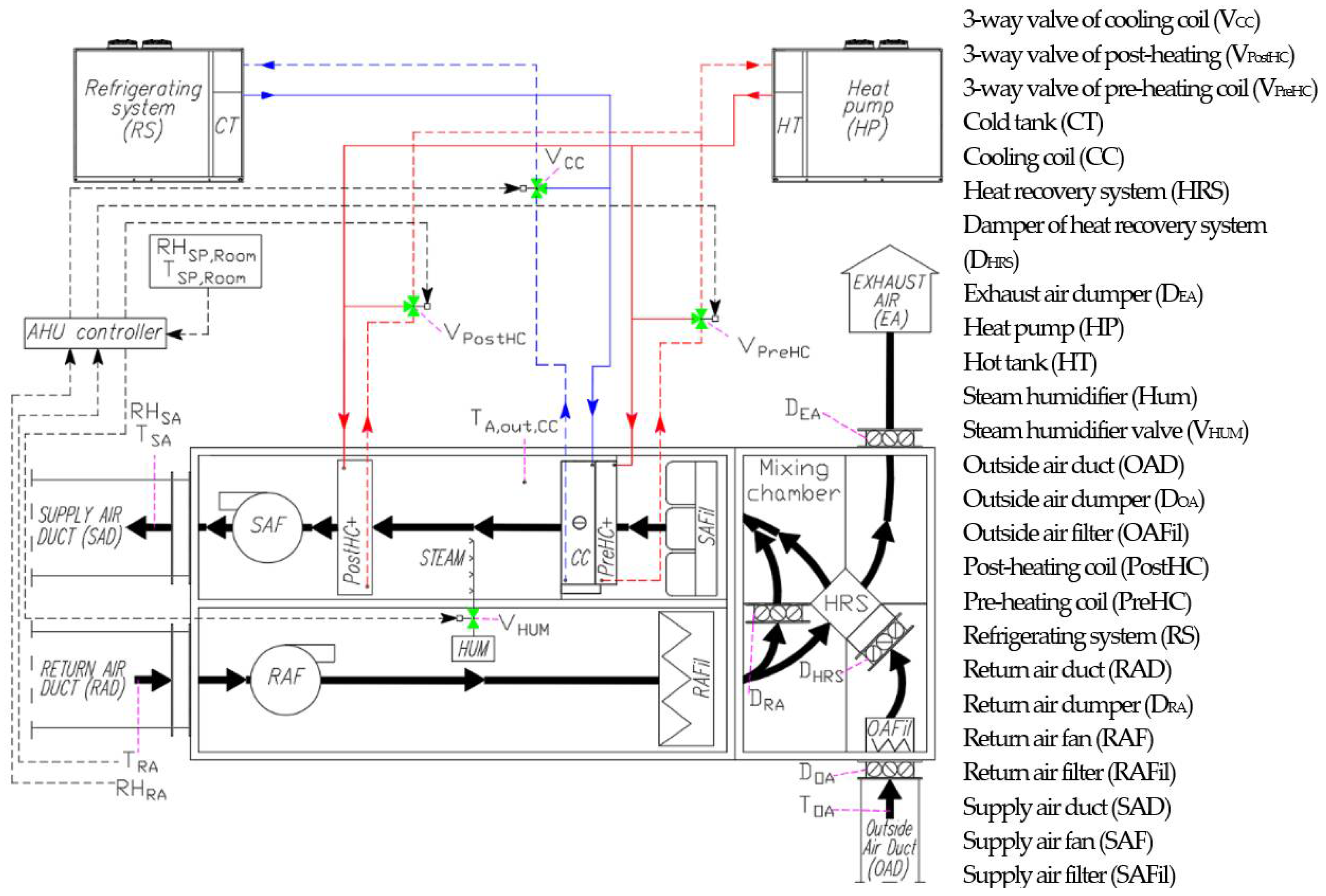
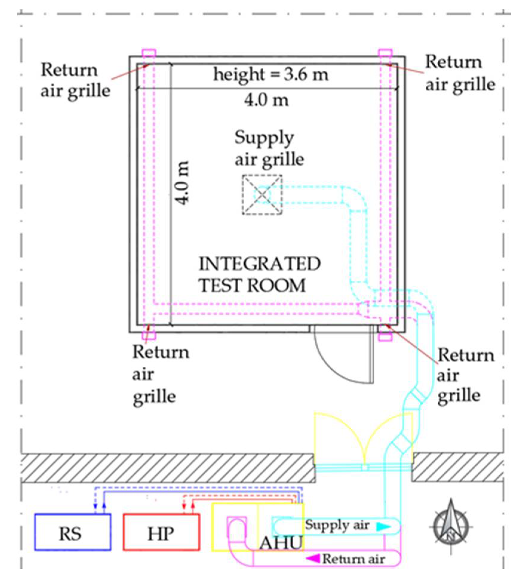
2. Description of the Experimental Setup

The SENS i-Lab is a multi-sensorial laboratory of the Department of Architecture and Industrial Design of the University of Campania Luigi Vanvitelli (Aversa, southern Italy, longitude: 14°12′26″ E, latitude: 40°58′21″ N). The SENS i-Lab consists of a human-centered, multi-physical, and multi-purpose test room served by an HVAC system, including a single duct dual-fan constant air volume (CAV) air handling unit, controlling indoor air temperature, indoor air relative humidity, indoor air velocity, and indoor air quality. The test room has a floor area of 16.0 m² (its height is 3.6 m) and four vertical walls (without windows and one door); both the ceiling and floor are horizontal. It is installed inside the Department, so that its indoor conditions are not directly affected by external climatic conditions.

Table A1. Properties of walls of the test room.

	Material (from Outside to Inside)	Thickness (m)	Thermal Conductivity (W/mK)	Thermal Resistance (m2K/W)		Heat Transfer Area (m2)
Ceiling	Plasterboard	0.0125	0.250	0.050	2.023	16.00
	Rock wool	0.0800	0.042	1.905
	Polyurethane panel	0.0150	0.220	0.068
Floor	Subfloor	0.1000	1.350	0.074	3.107	16.00
	Tiles	0.0500	2.100	0.024
	Polystyrene panel	0.0800	0.035	2.286
	Galvanized steel slab	0.0020	52.000	0.000
	Tiles	0.0100	1.050	0.010
West and East oriented vertical walls	Plasterboard	0.0125	0.250	0.050	2.005	14.40
	Rock wool	0.0800	0.042	1.905
	Radiant panel	0.0150	0.300	0.050
South and North oriented vertical walls	Plasterboard	0.0125	0.250	0.050	1.998	14.40
	Rock wool	0.0800	0.042	1.905
	Fiber-cement panel	0.0150	0.350	0.043
Door	Soft wood	0.0500	0.140	0.357	0.357	1.68

in Appendix A describes the material, thickness, thermal conductivity, conductive thermal resistance of each layer composing the walls, the ceiling, and the floor of the integrated test room.

A CAV AHU is commonly used in buildings; it is more common in existing old buildings or small new buildings, while in new medium/large buildings variable air volume (VAV) AHUs are the common choice of installation. In the case of CAV AHUs, volumetric flow rate of supply air is constant, while its supply temperature and relative humidity are varying. With respect to VAV AHUs, CAV AHUs are easier, cheaper, and quicker to install, but they are less efficient and with higher lifetime running costs. The AHU of the SENS i-Lab consists of these main functional subcomponents: return air fan (RAF); supply air fan (SAF); pre-heating coil (PreHC); post-heating coil (PostHC); cooling coil (CC); steam humidifier (HUM); static cross-flow heat recovery system (HRS); vapor compression air-to-water single-stage electric refrigerating system (RS) connected with the cooling coil; vapor-compression air-to-water single-stage electric heat pump (HP) connected with the pre-heating coil and the post-heating coil; valves (V_PreHC, V_PostHC, V_CC, V_HUM) controlling the flow rate of heat carrier fluid entering, respectively, the pre-heating coil, the post-heating coil, the cooling coil and the steam humidifier; return air damper (D_RA); outside air damper (D_OA); exhaust air damper (D_EA); damper of the HRS (D_HRS); return air filter (RAFil); outside air filter (OAFil); supply air filter (SAFil). Two 0.08 × 0.18 cm² air grilles are mounted on the south-oriented wall at floor level and two 0.08 × 0.18 cm² air grilles are mounted on the north-oriented wall at floor level with the aim of extracting air from indoor space to be moved into the AHU; a 0.60 × 0.60 cm² swirl diffuser acting as supply air grille is mounted on the ceiling of the test room. Figure 1 reports the scheme of the AHU together with its main components.

Figure A1 of Appendix A shows the floor plan of the test room including the AHU, together with the refrigerating system (RS), the heat pump (HP), as well as the return and supply air ducts.

Table 1. Main AHU components’ characteristics.

Supply air fan (SAF)	Maximum number of revolutions per minute (rpm)	3640
	Nominal velocity of supply air fan (%)	50
Return air fan (RAF)	Maximum number of revolutions per minute (rpm)	3080
	Nominal velocity of return air fan (%)	50
Cross flow heat recovery system (HRS)	Nominal recovery capacity (kW)	3.1
	Nominal efficiency (%)	74.7
	Nominal pressure drops on external/exhaust air side (kPa)	0.047/0.048
Return air filter (RAFil) and outside air filter (OAFil)	Type/Efficiency class	Fluted/G4
Supply air filter (SAFil)	Type/Efficiency class	Rigid pocket/G4
Return air duct (RAD) and supply air duct (SAD)	Diameter (m)	0.25
	Supply/Return length (m)	9.8/16.8
	Thermal resistance of insulating material (m2K/W)	0.25
Pre-heating coil (PreHC)	Nominal heating capacity (kW)	4.1
	Nominal air/fluid volumetric flow rate (m3/h)	600/0.710
	Nominal air/fluid pressure drops (kPa)	0.00321/12.43
Colling coil (CC)	Nominal cooling capacity (kW)	5.0
	Nominal air/fluid volumetric flow rate (m3/h)	600/0.860
	Nominal air/fluid pressure drops (kPa)	0.0178/13.56
Steam humidifier (HUM) [35]	Nominal steam capacity (kg/h)	5.0
	Nominal power (kW)	3.7
Post-heating coil (PostHC)	Nominal heating capacity (kW)	5.0
	Nominal air/fluid volumetric flow rate (m3/h)	600/0.860
	Nominal air/fluid pressure drops (kPa)	0.0497/20.35
Heat Pump (HP) [36]	Nominal capacity (kW)	14.0
	Nominal input power (kW)	4.75
	Nominal heat carrier fluid volumetric flow rate (m3/h)	2.41
Refrigerating System (RS) [36]	Nominal capacity (kW)	13.4
	Nominal input power (kW)	4.48
	Nominal heat carrier fluid volumetric flow rate (m3/h)	2.31

indicates the characteristics of the functional components of the HVAC serving the SENS i-Lab. The system fulfills the requirements prescribed by the Ecodesign Directive 1253/2014 [34] introduced by the European Union in order to support the diffusion of energy efficient AHUs. The HVAC unit is equipped with a number of sensors to observe and register the key operating system parameters. The measuring range as well as the accuracy of the sensors are showed in

Table 2. Measuring range and the accuracy of the AHU sensors.

Sensor Model	Monitored Parameter	Measuring Range	Accuracy
Siemens QFM2160 [37]	Return air temperature (TRA)	0 ÷ 50 °C	±0.8 °C
	Return air relative humidity (RHRA)	0 ÷ 100%	±3%
Siemens QFM2160 [37]	Supply air temperature (TSA)	0 ÷ 50 °C	±0.8 °C
	Supply air relative humidity (RHSA)	0 ÷ 100%	±3%
Siemens QAM2161.040 [38]	Outside air temperature (TOA)	−50 ÷ 50 °C	±0.75 °C
Siemens QAM2161.040 [38]	Cooling coil outlet air temperature (TA,out,CC)	−50 ÷ 50 °C	±0.75 °C
TSI 7575, 982 IAQ [39]	Temperature of air around the test room (TBEA)	−10 ÷ 60 °C	±0.50 °C
	Relative humidity of air around the test room (RHBEA)	5 ÷ 95%	±3%

.

The AHU is operated according to a specific control logic. In particular, the following parameters are manually set (and eventually modified during the test) by the end users: (i) the desired targets of both indoor relative humidity (RH_SP,Room) and indoor air temperature (T_SP,Room) to be reached and maintained into the test room; (ii) the deadband DB_T for T_SP,Room and the deadband DB_RH for RH_SP,Room; (iii) air flow rate of both the supply air fan (OL_SAF) and the return air fan (OL_RAF); (iv) opening percentages of the outside air damper (OP_DOA), the return air damper (OP_DRA), and the exhaust air damper (OP_DEA); and (v) activation of the heat recovery system damper (OP_DHRS). Flow rate of air moved by the supply air fan can range between 0 (OL_SAF = 0%) and 1080 m³/h (OL_SAF = 100%), while flow rate of air moved by the return air fan is between 0 (OL_RAF = 0%) and 1460 m³/h (OL_RAF = 100%); the maximum electric consumption of the SAF and RAF are, respectively, 1.22 kW and 0.48 kW. The parameter OP_DHRS can be fixed at 100% (no heat recovery) or 0% (heat recovery takes place). The variation range of the parameters OP_DRA, OP_DOA, and OP_DEA is 0÷100% (100% corresponds to the dampers fully open). Once the previous parameters are manually set by the end-users, opening percentages of the valves (OP_{V_PreHC}, OP_{V_PostHC}, OP_{V_CC} and OP_{V_HUM}) are automatically managed in the range 0 ÷ 100% by proportional-integral-derivative (PID) controllers in order to achieve the indoor desired targets. Opening percentages of the valves are continuously regulated between 0% and 100% as a function of differences between the targets of air temperature and relative humidity into the test room and their current values. In more detail, volumetric flow rate of fluid streaming inside the coils can be modulated between 0 and 0.860 m³/h, while flow rate of steam mass of the steam humidifier can be varied from 0 up to 5 kg/h.

Table 3. Activation criteria of the AHU’s components.

Component of AHU	ON	OFF
Steam humidifier (HUM)	RHRA ≤ (RHSP,Room − DBRH)	RHRA ≥ (RHSP,Room + DBRH)
Cooling coil (CC)	TRA ≥ (TSP,Room + DBT) OR RHRA ≥ (RHSP,Room + DBRH)	TRA ≤ (TSP,Room − DBT) AND RHRA ≤ (RHSP,Room − DBRH)
Post-heating coil (PostHC)	TRA ≤ (TSP,Room − DBT)	TRA ≥ (TSP,Room + DBT)
Heat Pump (HP) [36]	THT < 44 °C	THT ≥ 46 °C
Refrigerating System (RS) [36]	TCT > 8 °C	TCT ≤ 6 °C

reports the main criteria for activating and deactivating the main functional subsystems of the AHU serving the test room. The pre-heating coil is not included in the table because this subsystem has been kept deactivated during the entire duration of all experimental tests. The post-heating coil is activated when return air temperature becomes not larger than the temperature difference (T_SP,Room − DB_T), while it is deactivated in the case of T_RA assumes a value not lower than the temperature (T_SP,Room + DB_T). The cooling coil is activated when return air temperature becomes not lower than the temperature (T_SP,Room + DB_T), while it is deactivated in the case of T_RA assumes a value not larger than the temperature difference (T_SP,Room − DB_T). The steam humidifier is activated when return air relative humidity becomes not larger than the air relative humidity difference (RH_SP,Room − DB_RH), while it is deactivated in the case of RH_RA assumes a value not lower than the air relative humidity (RH_SP,Room + DB_RH). The heat pump is activated when temperature into the hot tank T_HT is lower than 44 °C, while it is deactivated in the case of T_HT assumes a value not lower than 46 °C. The refrigerating device is activated when the temperature into the cold tank T_CT is larger than 8 °C, while it is deactivated in the case that T_CT assumes a value not larger than 6 °C. The signals managing the opening percentages of the valves (OP_{V_PreHC,} OP_{V_PostHC}, OP_{V_CC}, and OP_{V_HUM}) are generated by PID controllers. As an alternative to the automatic operation based on PID controllers, the opening percentages of the valves (OP_{V_PreHC,} OP_{V_PostHC}, OP_{V_CC}, and OP_{V_HUM}) can be also forced by the end-users; therefore, the end user is allowed to force component operation/parameters based on specific research purposes.

However, alternatively, the end users can also manually force (at the beginning or during the test) the opening percentages of the valves for research purposes (instead of operating according to the automatic control logic).

3. Experimental Tests

A set of 18 fault-free and faulty daily experimental tests has been performed in order to examine the HVAC system operation during transient and steady-state operation under both winter and summer conditions.

Table 4. Operating conditions of the experimental tests under fault free (tests 1–4) and faulty operation (tests 5–9) during summer.

Test n.	TSP,Room (°C)	RHSP,Room (%)	TOA (°C)	OLRAF (%)	OLSAF (%)	OPV_PostHC (%)	OPV_CC (%)	OPV_HUM (%)	Date (dd/mm/yyyy)
1	26	50	20.6 ÷ 26.7	50	50	0 ÷ 100	0 ÷ 100	0 ÷ 100	29/06/2020
2	26	50	29.1 ÷ 35.2	50	50	0 ÷ 100	0 ÷ 100	0 ÷ 100	28/07/2020
3	26	50	25.3 ÷ 32.0	50	50	0 ÷ 100	0 ÷ 100	0 ÷ 100	23/07/2020
4	26	50	28.6 ÷ 35.3	50	50	0 ÷ 100	0 ÷ 100	0 ÷ 100	21/07/2020
5 (fault1)	26	50	30.4 ÷ 34.9	50	20	0 ÷ 100	0 ÷ 100	0 ÷ 100	31/07/2020
6 (fault2)	26	50	32.1 ÷ 38.8	20	50	0 ÷ 100	0 ÷ 100	0 ÷ 100	03/08/2020
7 (fault3)	26	50	33.8 ÷ 38.4	50	50	0	0 ÷ 100	0 ÷ 100	16/09/2020
8 (fault4)	26	50	29.4 ÷ 35.8	50	50	0 ÷ 100	0	0 ÷ 100	16/09/2020
9 (fault5)	26	50	28.7 ÷ 38.2	50	50	0 ÷ 100	0 ÷ 100	0	18/09/2020

and

Table 5. Operating conditions of the experimental tests under fault free (tests 10–13) and faulty operation (test 14–18) during winter.

Test n.	TSP,Room (°C)	RHSP,Room (%)	TOA (°C)	OLRAF (%)	OLSAF (%)	OPV_PostHC (%)	OPV_CC (%)	OPV_HUM (%)	Date (dd/mm/yyyy)
10	20	50	10.3 ÷ 15.0	50	50	0 ÷ 100	0 ÷ 100	0 ÷ 100	23/12/2020
11	20	50	13.2 ÷ 15.4	50	50	0 ÷ 100	0 ÷ 100	0 ÷ 100	28/12/2020
12	20	50	12.7 ÷ 18.6	50	50	0 ÷ 100	0 ÷ 100	0 ÷ 100	29/12/2020
13	20	50	8.0 ÷ 13.5	50	50	0 ÷ 100	0 ÷ 100	0 ÷ 100	05/01/2021
14 (fault1)	20	50	12.3 ÷ 20.0	50	20	0 ÷ 100	0 ÷ 100	0 ÷ 100	12/01/2021
15 (fault2)	20	50	5.6 ÷ 12.2	20	50	0 ÷ 100	0 ÷ 100	0 ÷ 100	14/01/2021
16 (fault3)	20	50	10.5 ÷ 15.9	50	50	0	0 ÷ 100	0 ÷ 100	28/01/2021
17 (fault4)	20	50	7.8 ÷ 16.8	50	50	0 ÷ 100	0	0 ÷ 100	15/02/2021
18 (fault5)	20	50	9.2 ÷ 13.3	50	50	0 ÷ 100	0 ÷ 100	0	12/02/2021

describe the operating of the experimental tests under summer and winter conditions, respectively.

During all the tests, a number of system parameters have been kept constant: DB_T = 1 °C, DB_RH = 5%, OP_DRA = 100%, OP_DOA = 20%, OP_DEA = 20%, and OP_DHRS = 100. In more detail, 8 tests have been performed under fault free conditions (tests n. 1, 2, 3, 4 in Table 4 carried out during summer and tests n. 10, 11, 12, 13 in Table 5 carried out during winter). The remaining 10 tests have been carried out while artificially introducing specific faults (tests n. 5, 6, 7, 8, 9 in Table 4 carried out during summer and tests n. 14, 15, 16, 17, 18 in Table 5 carried out during winter). The experiments have been performed by measuring every minute all the parameters indicated in Table 2. In this study, the recording time step of measured data has been defined according to the experimental approaches adopted in similar works available in the scientific literature. For example, the ASHRAE RP-1312 data set [24] developed for AFDD purposes consists of experimental data recorded every minute from a facility comprising two AHUs; recently, Piscitelli et al. [5], Yun et al. [27], as well as Fan et al. [28] proposed novel methodologies for performing AFDD analyses of AHUs based on this ASHRAE RP-1312 database [24]; Cheng et al. [40] developed a new AFDD method for AHUs using experimental data measured every minute. Therefore, a measurement time step of one minute could be reasonably assumed as acceptable in order to take into account the response time of HVAC components.

Only during the faulty tests, the operation of specific AHU components has been forced to assure user-specified positions in order to artificially simulate the following 5 specific typical faults (named fault 1, 2, 3, 4, 5):

• Fault 1 has been implemented during both the tests n. 5 and n. 14, i.e., the velocity of the supply air fan has been kept at 20% (instead of the nominal value of 50%);
• Fault 2 has been implemented during both the tests n. 6 and n. 15, i.e., the velocity of the return air fan has been kept at 20% (instead of the nominal value of 50%);
• Fault 3 has been implemented during both the tests n. 7 and 16, i.e., the valve managing the flow rate entering the post-heating coil has always been kept closed (instead of allowing its normal operation with an opening percentage in the range 0 ÷ 100% according to the AHU automatic control logic);
• Fault 4 has been implemented during both the tests n. 8 and n. 17, i.e., the valve managing the flow rate entering the cooling coil has always been kept closed (instead of allowing its normal operation with an opening percentage in the range 0 ÷ 100% according to the AHU automatic control logic);
• Fault 5 has been implemented during both the tests n. 9 and n. 18, i.e., opening percentage of the valve managing the flow rate entering the steam humidifier has always been kept closed (instead of allowing its normal operation with an opening percentage in the range 0 ÷ 100% according to the AHU automatic control logic).

In this study, the above-mentioned faults have been introduced at the beginning of the faulty tests and maintained during the entire duration of the experiments (what happens in the case of the faults are shorter has not been investigated).

During the tests n. 1–4 and n. 10–13 (fault free tests), the AHU’s components have been operated without any artificial faults.

In both Table 4 and Table 5, the parameters characterizing the corresponding faults have been highlighted in red.

Figure 2a–d and Figure 3a–e highlight the experimental trends of return air temperature T_RA, supply air temperature T_SA, outside air temperature T_OA, air temperature around the test room T_BEA, return air relative humidity RH_RA, supply air relative humidity RH_SA, and air relative humidity around the test room RH_BEA recorded during the fault free and faulty tests, respectively, performed under summer conditions (detailed in Table 4).

Figure 2a reports the experimental trends of T_RA, T_SA, T_OA, T_BEA, RH_RA, RH_SA, RH_BEA during the fault free test n.1; Figure 2b shows the measured parameters T_RA, T_SA, T_OA, T_BEA, RH_RA, RH_SA, RH_BEA during the fault free test n.2; Figure 2c indicates the measured data associated to T_RA, T_SA, T_OA, T_BEA, RH_RA, RH_SA, RH_BEA during the fault free test n.3; Figure 2d highlights the temporal variation of T_RA, T_SA, T_OA, T_BEA, RH_RA, RH_SA, RH_BEA during the fault free test n.4.

Figure 3a reports the experimental trends of T_RA, T_SA, T_OA, T_BEA, RH_RA, RH_SA, RH_BEA during the faulty test n.5; Figure 3b shows the measured parameters T_RA, T_SA, T_OA, T_BEA, RH_RA, RH_SA, RH_BEA during the faulty test n.6; Figure 3c indicates the measured data associated to T_RA, T_SA, T_OA, T_BEA, RH_RA, RH_SA, RH_BEA during the faulty test n.7; Figure 3d highlight the temporal variation of T_RA, T_SA, T_OA, T_BEA, RH_RA, RH_SA, RH_BEA during the faulty test n.8; the values of T_RA, T_SA, T_OA, T_BEA, RH_RA, RH_SA, RH_BEA recorded during the faulty test n.9 are depicted in Figure 3e.

Figure 4a–d and Figure 5a–e report the experimental trends of T_RA, T_SA, T_OA, T_BEA, RH_RA, RH_SA, RH_BEA recorded during the fault free and faulty tests, respectively, performed under winter conditions (detailed in Table 5).

Figure 4a reports the experimental trends of T_RA, T_SA, T_OA, T_BEA, RH_RA, RH_SA, RH_BEA during the fault free test n.10; Figure 4b shows the measured parameters T_RA, T_SA, T_OA, T_BEA, RH_RA, RH_SA, RH_BEA during the fault free test n.11; Figure 4c indicates the measured data associated to T_RA, T_SA, T_OA, T_BEA, RH_RA, RH_SA, RH_BEA during the fault free test n.12; Figure 4d highlights the temporal variation of T_RA, T_SA, T_OA, T_BEA, RH_RA, RH_SA, RH_BEA during the fault free test n.13.

Figure 5a reports the experimental trends of T_RA, T_SA, T_OA, T_BEA, RH_RA, RH_SA, RH_BEA during the faulty test n.14; Figure 5b shows the measured parameters T_RA, T_SA, T_OA, T_BEA, RH_RA, RH_SA, RH_BEA during the faulty test n.15; Figure 5c indicates the measured data associated to T_RA, T_SA, T_OA, T_BEA, RH_RA, RH_SA, RH_BEA during the faulty test n.16; Figure 5d highlight the temporal variation of T_RA, T_SA, T_OA, T_BEA, RH_RA, RH_SA, RH_BEA during the faulty test n.17; the values of T_RA, T_SA, T_OA, T_BEA, RH_RA, RH_SA, RH_BEA recorded during the faulty test n.18 are depicted in Figure 5e.

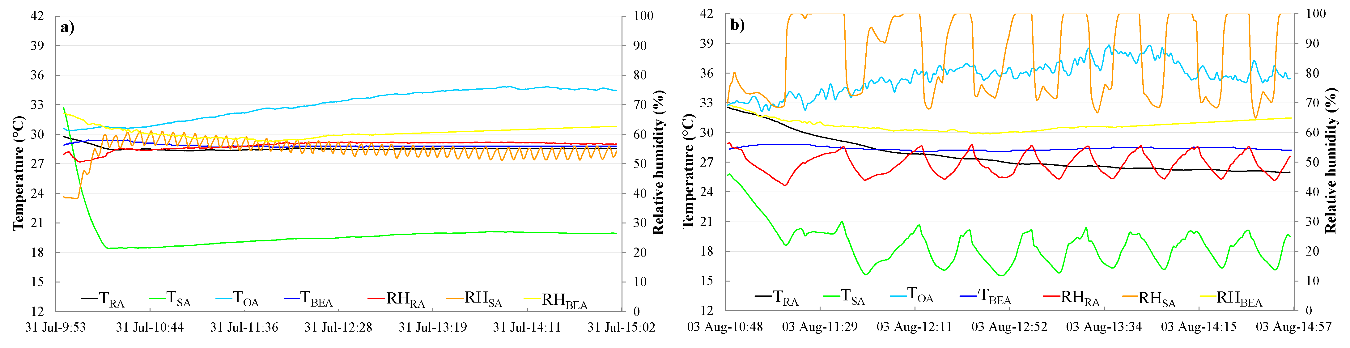
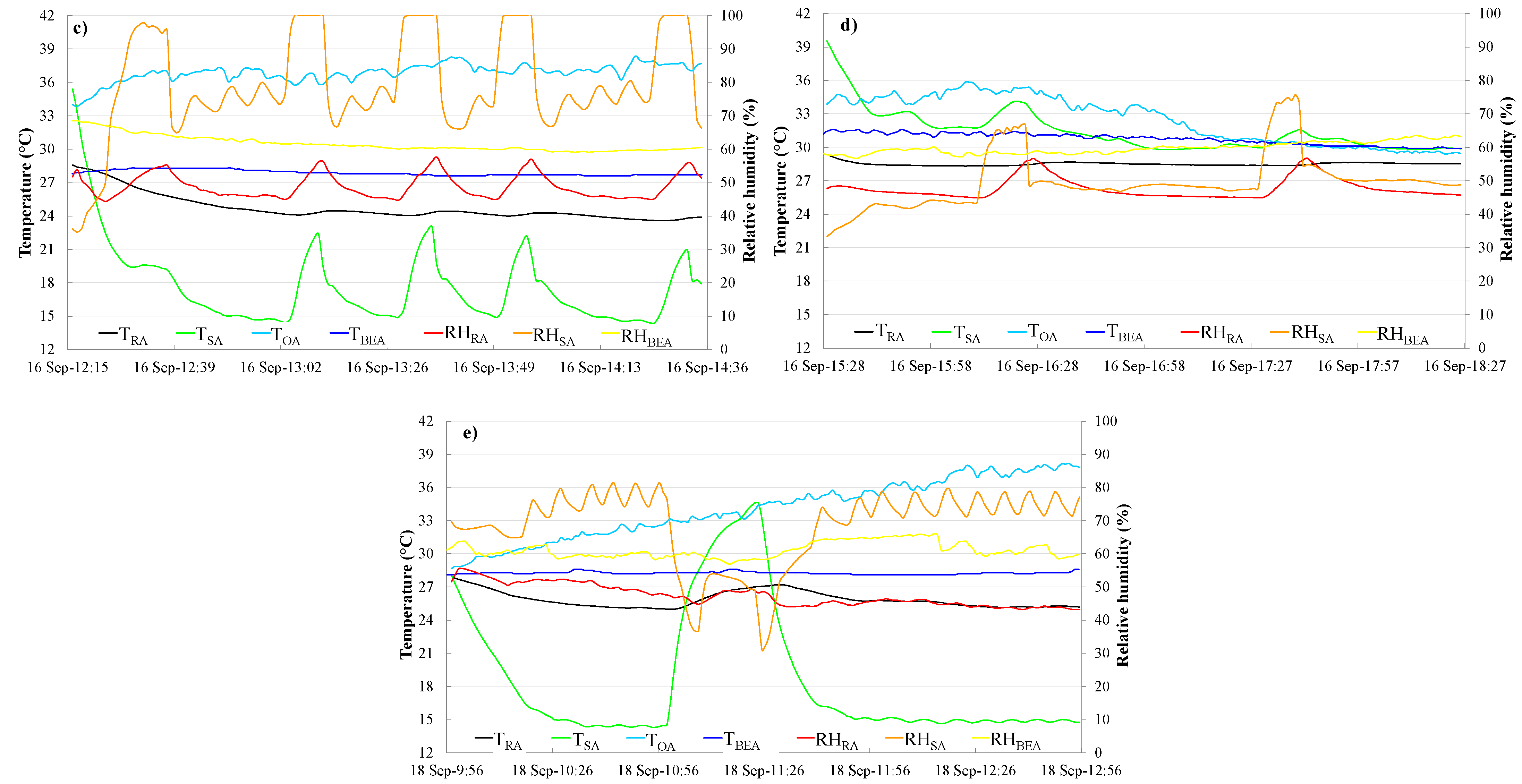
Analysis of Experimental Trends

The data acquired during normal and faulty operation tests (and reported in previous section) highlight that the percentages of time with values of indoor air temperature within the given deadband (1 °C) around the user-defined target (setpoint 26/20 °C for summer/winter season) are equal to 69.8%, 57.0%, 71.3%, 69.1%, 0%, 36.1%, 13.4%, 0%,86.6%, 68.3%, 69.6%, 72.5%, 71.4%, 75.4%, 68.7%, 0.0%, 15.7%, and 64.9% for the tests 1–18, respectively. Furthermore, the percentages of time with values of air relative humidity inside the test room within the deadband (5%) around the target (50%) are equal to 98.4%, 84.9%, 83.5%, 88.3%, 16.2%, 80.6%, 88.1%, 90.6%, 65.4%, 84.7%, 80.7%, 87.3%, 81.2%, 49.4%, 82.3%, 99.6%, 80.5%, and 76.0%, during the tests 1–18, respectively. The results of calculation highlight a good capability of the HVAC unit under healthy operation (tests n. 1–4 and 10–13) to accurately control indoor conditions. The previously mentioned percentages are lower than 100% because (a) the initial values of return air temperature and return air relative humidity are in some cases far from target values and (b) during the start-up phases the AHU operates under transient conditions trying to approach the steady-state conditions to achieve the desired targets.

In more detail, Figure 3a–e (associated to the faulty tests performed during summer) highlights the different trends/patterns associated to key operating parameters with respect to the scenarios without faults:

• In Figure 3a (corresponding to the fault 1, i.e., velocity of the supply air fan reduced at 20%), supply air temperature and supply air relative humidity are in a much narrower range as it would expected in the case of reduced supply air flow; in this case, T_SA drops to about 18.4 °C and then it remains below 20.5 °C (out of the desired thermal comfort range) during the remaining part of the test, while RH_SA is in the range of 51% to 61% with a larger number of oscillations; in addition, it can be noticed that both return air temperature T_RA and return air relative humidity RH_RA vary much more slowly as a function of time;
• Figure 3b (corresponding to the fault 2, i.e., velocity of the return air fan reduced at 20%) indicates that, as supposed, supply air temperature varies in a smaller range (in this case between 15.5 °C and 21.0 °C) when return air flow rate is reduced;
• In Figure 3c (corresponding to the fault 3, i.e., post-heating coil valve kept fully closed), supply air temperature T_SA assumes lower average values, ranging in a narrower interval (in this case between 14.5 °C and 23.0 °C) due to the fact that post-heating coil is not active; as a consequence, return air temperature, after the initial drop from ~28.5 °C down to ~24.0 °C, remains almost constant during the remaining part of the test (with a value smaller than its lower deadband and, therefore, out of desired thermal comfort range); in addition, it should be underlined that average values of supply air relative humidity are greater;
• In Figure 3d (corresponding to the fault 4, i.e., cooling coil valve kept fully closed), supply air temperature is characterized by much larger average values (as it would be expected due to the missing contribution of the cooling coil), with a narrower variation range (in this case between 30.0 °C and 34.0 °C); return air temperature is substantially constant, assuming a value larger than its upper deadband (in this case equal to ~28.5 °C) and, therefore, out of the desired thermal comfort range;
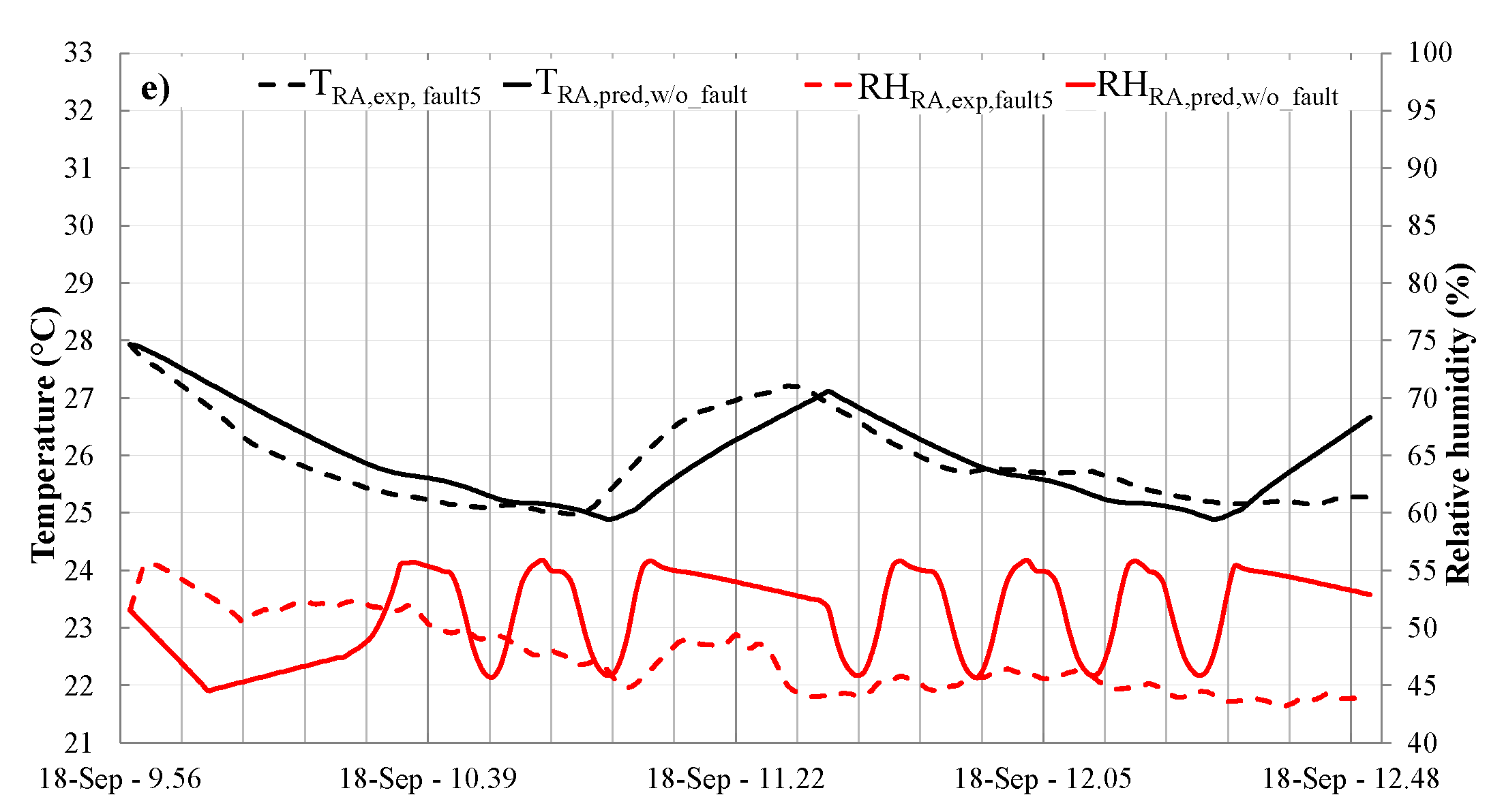
• In Figure 3e (corresponding to the fault 5, i.e., steam humidifier valve kept fully closed), return air relative humidity varies in a narrower range (in this case between 43.0% and 55.5%), highlighting a significantly reduced number of oscillations (as it would be presumed in the case of the humidifier is not active).

Figure 5a–e (associated to the faulty tests performed during winter) allows to underline the different trends/patterns of key operating parameters with respect to the cases without faults:

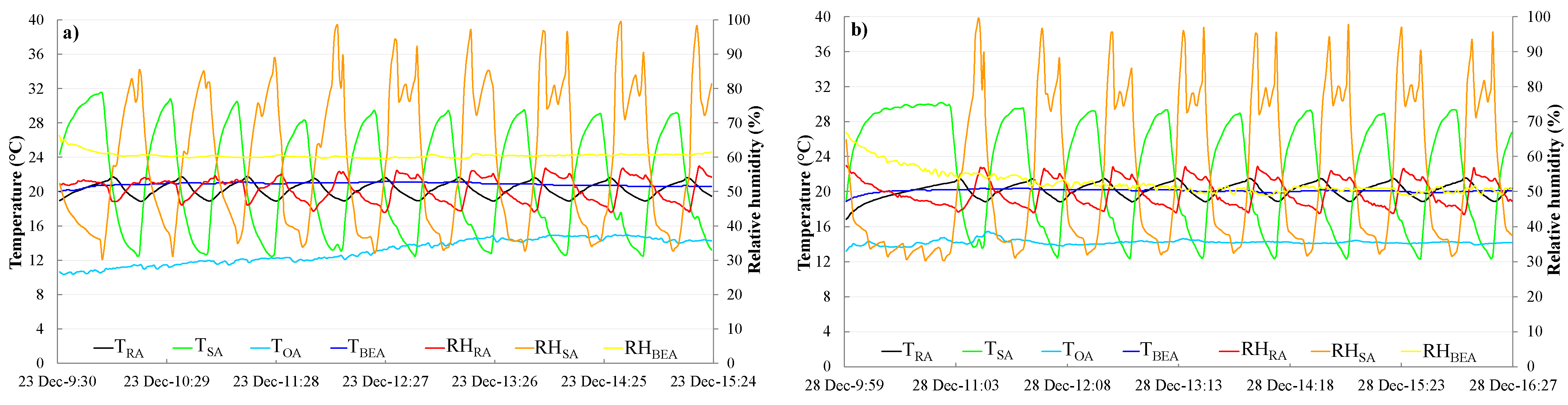
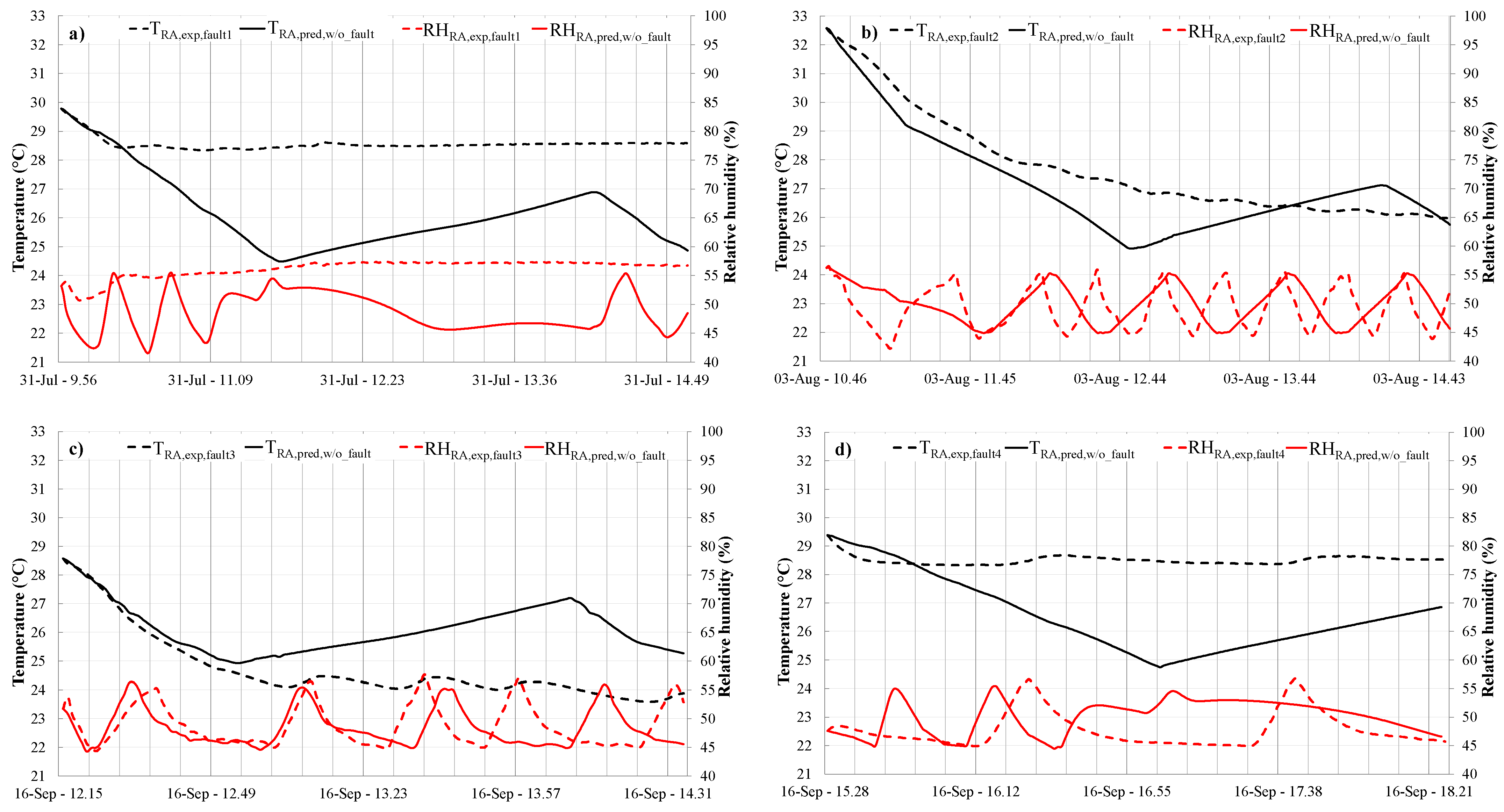
• In Figure 5a (corresponding to the fault 1, i.e., velocity of the supply air fan reduced at 20%), the supply air temperature and supply air relative humidity are in a wider range, with a much lower number of oscillations; similar trends can be recognized for both return air temperature and return air relative humidity;
• Figure 5b (corresponding to the fault 2, i.e., velocity of the return air fan reduced at 20%) indicates that the impact of a reduced return ai flow rate is almost negligible in terms of supply and return air temperature as well as supply and return air relative humidity;
• In Figure 5c (corresponding to the fault 3, i.e., post-heating coil valve kept fully closed), supply air temperature assumes lower average values (as post-heating coil is not active); in particular, T_SA is almost constant (and equal to ~12.0 °C in this case). As a consequence, return air temperature remains almost constant during the test, assuming a value much smaller than its lower deadband and, therefore, out of the desired thermal comfort range. In addition, it should be underlined that average values of supply air relative humidity are greater and included in a narrower range (without significant oscillations); return air relative humidity is almost constant (and equal to about 47% in this case);
• In Figure 5d (corresponding to the fault 4, i.e., cooling coil valve kept fully closed), supply air temperature is characterized by lower average values (as it would be presumed due to the missing contribution of the cooling coil), with a narrower variation range (approximately 19.0–24.0 °C in this case); return air temperature is substantially constant, assuming a value out of desired thermal comfort range (slightly larger than its upper deadband and equal to about 22.0 °C in this case);
• In Figure 5e (corresponding to the fault 5, i.e., steam humidifier valve kept fully closed), return air relative humidity varies in a slightly narrower range (as it would be expected in the case of the humidifier is not active).

4. Simulation Model

In this paper, an artificial neural network (ANN)-based model has been developed in the MATLAB environment. The aim was to predict (i) the supply air temperature, (ii) the supply air relative humidity, (iii) the opening percentage of the valve supplying the post-heating coil, (iv) the opening percentage of cooling coil valve, and (v) the opening percentage of the steam humidifier valve. This ANN has been first validated with measured data and then coupled with a dynamic simulation model developed in TRNSYS environment in order to simulate (i) the return air temperature; (ii) the return air relative humidity; as well as (iii) the electric energy consumptions (not measured) of the heat pump, the refrigerating system, the steam humidifier, the supply air fan, and the return air fan with the aim of rating the effects of the selected faults on both energy consumption as well occupant indoor thermo-hygrometric comfort. The artificial neural network-based model is described in Section 4.1, Section 4.1.1, Section 4.1.2 and Section 4.1.3, while the description of the TRNSYS model is reported in Section 4.2.

4.1. Artificial Neural Network-Based Model

In this section, the ANN-based models developed with the aim of simulating the performance of the test room-integrated HVAC system under both normal and faulty scenarios are described.

4.1.1. Artificial Neural Networks’ Architecture

ANNs usually consist of three parts: one input layer; one or more hidden layers, and one output layer. All layers include neurons, and each neuron in a given layer is linked to the neurons of previous as well as successive layers. Each link between two neurons is characterized by an adaptable synaptic weight and bias. Three main different functional operations occur in ANNs:

• all the inputs are multiplied by their weights;
• the weighted values are added to the bias in order to form the net inputs;
• the net inputs are passed by means of the transfer function, which generates the outputs.

ANNs are trained by means of a suitable learning method in order to obtain a specific target output from a particular input by regulating the weights and biases. The training process is stopped only when the error between the desired target and the corresponding network output is lower than a given tolerance value or when the maximum number of epochs (given number of iterations) is achieved. A transfer function is a mathematical representation of the relation between inputs and outputs. Transfer functions generally have a sigmoid shape, but they may also assume the form of piecewise linear functions, nonlinear functions, or step functions. One of the most commonly adopted transfer functions for multilayer networks is the hyperbolic tangent sigmoid transfer function (tansig) [32] generating outputs between −1 and 1.

Performance of artificial neural networks is sensitive to both the number of hidden layers as well as the number of neurons in their hidden layers [32]. In particular, networks with more hidden layers require a larger computation time, but their use gives the network more flexibility and could result in resolving challenging tasks more efficiently [32]. Larger numbers of neurons allow the network to figure out more difficult issues; however, they require more computation and they can play a part to “overfitting” (in that case the fitting curve fluctuates wildly among training points, even if these points are well fitted); on the other hand, few neurons can reduce the computation time, but they could also lead to “underfitting”.

The MATLAB (The MathWorks Inc., Natick, Massachusetts, USA) Neural Network Toolbox [32] has been used in this work in order to develop and analyze 22 artificial neural network-based simulation models (ANN1-ANN22) of the HVAC system. All the artificial neural networks have been configured with 10 inputs and 5 outputs, varying the number of hidden layers and neurons in each hidden layer. One of the most common issues to be addressed in configuring the architecture of ANNs is connected to the ANNs topology allowing to achieve the requested accuracy and/or minimize the computation time. Several studies [41,42,43,44,45,46] have determined the number of hidden layers and the number of neurons in the hidden layers by trial and error, employing a grid search technique to find them. A sensitivity analysis has been performed in this study in order to find out the optimal number of hidden layers and neurons in each hidden layer according to the information and approaches reported in the current literature. In particular, several scientific papers investigated the application of ANNs for HVAC systems’ modeling [41,42,43], adopting a number of hidden layers varying from a minimum of 1 [41] up to a maximum of 5 [41,42,43]. In addition, several formulas are available in the scientific literature [44,45,46] in order to provide a starting point for determining the optimal number of neurons in each hidden layer of ANNs as a function of (i) number of inputs [44,45,46], (ii) number of outputs [44], (iii) number of hidden layers [45], and (iv) number of training examples [45,46]; these formulas suggest a number of neurons per hidden layer in the range of 7 to 83 when applied to the ANNs investigated in this paper.

4.1.2. Sensitivity Analysis of Artificial Neural Networks

Table 6. Architectures of the investigated ANNs.

ANN ID	Number of Hidden Layers	Number of Neurons in Each Hidden Layer
ANN1	1	10
ANN2	1	20
ANN3	1	30
ANN4	1	40
ANN5	1	50
ANN6	1	60
ANN7	1	70
ANN8	2	10
ANN9	2	20
ANN10	2	30
ANN11	2	40
ANN12	2	50
ANN13	3	10
ANN14	3	20
ANN15	3	30
ANN16	3	40
ANN17	4	10
ANN18	4	20
ANN19	4	30
ANN20	5	10
ANN21	5	20
ANN22	5	30

describes the architectures of the 22 ANN-based models investigated in this paper, highlighting both number of hidden layers as well as number of neurons in each hidden layer.

The following 10 variables have been set as inputs of all ANNs:

• difference between current return air temperature and related target (ΔT)
• difference between current return air relative humidity and related target (ΔRH)
• supply air temperature at previous minute (T_SA-1)
• supply air relative humidity at previous minute (RH_SA-1)
• outside air temperature (T_OA)
• opening percentage of the valve managing the flow entering the post-heating coil at previous minute (OP_{V_PostHC-1})
• opening percentage of the valve managing the flow entering the cooling coil at previous minute (OP_{V_CC-1})
• opening percentage of the valve managing the flow entering the steam humidifier at previous minute (OP_{V_HUM-1})
• supply air fan velocity (OL_SAF)
• return air fan velocity (OL_RAF).

The following five parameters have been set as outputs of all ANNs:

• supply air temperature (T_SA)
• supply air relative humidity (RH_SA)
• opening percentage of the post-heating coil valve (OP_{V_PostHC})
• opening percentage of the cooling coil valve (OP_{V_CC})
• opening percentage of the steam humidifier valve (OP_{V_HUM}).

Table 7. Inputs and outputs of the ANNs.

Number of Inputs	Input ID	Number of Outputs	Outputs ID
1	ΔT	1	TSA
2	ΔRH
3	TSA-1	2	RHSA
4	RHSA-1
5	TOA	3	OPV_PostHC
6	OPV_PostHC-1
7	OPV_CC-1	4	OPV_CC
8	OPV_HUM-1
9	OLSAF	5	OPV_HUM
10	OLRAF

summarizes the inputs and the outputs used in the artificial neural networks. Each ANN has 1 input layer with 10 neurons and 1 output layer with 5 neurons.

The hyperbolic tangent sigmoid transfer function (tansig) has been adopted in the hidden and output layers of each ANN. Levenberg–Marquart back-propagation training algorithms (trainlm) have been selected as training function with the aim of updating the weights and biases.

4.1.3. Training, Testing and Validation of ANNs

The experimental data measured during the tests described in Section 3 have been used for training, testing, and validating the ANNs. Two different datasets have been randomly extracted from the entire database (5352 data points in total): the first dataset (3746 points) has been utilized for training purposes, while the second one (1606 points) has been considered for testing and validating the networks. The predictions of the ANN-based models have been compared with the whole experimental dataset (containing all training, testing, and validation points) to evaluate the reliability of the ANNs by means of the metrics reported below (the average error $\overline{\mathsf{\epsilon }}$, the average absolute error $\left|\overline{\mathsf{\epsilon }}\right|$, the mean square error MSE, the root mean square error RMSE, and the coefficient of determination R²):

$${\mathsf{\epsilon }}_{\mathrm{i}}{=\mathrm{g}}_{\mathrm{pred},\mathrm{i}}{-\mathrm{g}}_{\exp ,\mathrm{i}}$$

(1)

$$\overline{\mathsf{\epsilon }}={\displaystyle \sum _{\mathrm{i}=1}^{\mathrm{N}}{\mathsf{\epsilon }}_{\mathrm{i}}/\mathrm{N}}$$

(2)

$$\left|\overline{\mathsf{\epsilon }}\right|={\displaystyle \sum _{\mathrm{i}=1}^{\mathrm{N}}\left|{\mathsf{\epsilon }}_{\mathrm{i}}\right|}/\mathrm{N}$$

(3)

$$\mathrm{MSE}=\frac{1}{\mathrm{N}}{{\displaystyle \sum _{\mathrm{i}=1}^{\mathrm{N}}\left({\mathsf{\epsilon }}_{\mathrm{i}}-\overline{\mathsf{\epsilon }}\right)}}^2$$

(4)

$$\mathrm{RMSE}=\sqrt{{\displaystyle \sum _{\mathrm{i}=1}^{\mathrm{N}}\frac{{\left({\mathsf{\epsilon }}_{\mathrm{i}}-\overline{\mathsf{\epsilon }}\right)}^2}{\mathrm{N}}}}$$

(5)

$${\mathrm{R}}^2=1-\left[{\displaystyle \sum _{\mathrm{i}=1}^{\mathrm{N}}\frac{{\left({\mathrm{g}}_{\exp ,\mathrm{i}}-{\mathrm{g}}_{\mathrm{pred},\mathrm{i}}\right)}^2}{{\left({\mathrm{g}}_{\exp ,\mathrm{i}}-{\overline{\mathrm{g}}}_{\mathrm{pred},\mathrm{i}}\right)}^2}}\right]$$

(6)

where N is the total number of experimental points, while g_pred,i, g_exp,I, and $\overline{\mathrm{g}}$_pred are, respectively, the predictions at time step i, the measurements at time step i, and the arithmetic mean of the predicted values.

Table 8. Errors between predictions of ANN-based models and measurements.

Errors	ANN Outputs	ANN1	ANN2	ANN3	ANN4	ANN5	ANN6	ANN7	ANN8	ANN9	ANN10	ANN11	ANN12	ANN13	ANN14	ANN15	ANN16	ANN17	ANN18	ANN19	ANN20	ANN21	ANN22
$\overline{\mathsf{\epsilon }}$	TSA (°C)	−0.11	−0.03	0.00	−0.01	−0.01	−0.01	−0.01	0.00	−0.01	0.00	0.05	−0.01	−0.09	0.00	0.01	0.00	0.00	0.04	−0.02	0.02	10.71	−0.01
	RHSA (%)	0.22	−0.02	0.10	0.08	0.04	−0.06	0.04	−0.03	0.06	−0.02	−0.24	0.06	0.18	0.05	0.00	−0.01	−0.04	0.02	−0.05	−0.02	0.01	0.01
	OPV_PostHC (%)	0.00	0.01	0.00	0.01	0.00	0.01	−0.01	−0.01	0.00	0.01	0.00	0.00	0.00	−0.01	−0.01	0.02	0.00	0.01	−0.01	0.00	3.66	−0.01
	OPV_CC (%)	0.00	−0.02	0.00	0.06	0.01	0.04	0.01	−0.02	0.01	0.02	−0.02	−0.01	−0.03	0.00	0.02	0.01	−0.03	0.01	−2.48	0.00	0.02	0.01
	OPV_HUM (%)	0.01	0.00	−0.03	0.04	−0.01	−0.02	−0.02	0.01	−0.01	−0.02	−0.02	−0.02	0.03	−0.03	0.01	0.01	0.07	0.00	0.03	0.03	−0.02	0.01
$\left|\overline{\mathsf{\epsilon }}\right|$	TSA (°C)	0.72	0.36	0.36	0.36	0.31	0.26	0.25	0.62	0.41	0.42	0.44	0.34	0.70	0.47	0.43	0.27	0.72	0.46	0.45	0.69	10.71	0.36
	RHSA (%)	2.80	2.00	2.00	1.95	1.80	1.67	1.75	2.32	2.02	1.98	1.99	1.77	2.46	2.13	1.94	1.62	2.26	2.00	1.88	2.57	2.00	1.83
	OPV_PostHC (%)	0.08	0.06	0.08	0.19	0.12	0.10	0.12	0.06	0.06	0.20	0.13	0.11	0.07	0.10	0.13	0.06	0.05	0.11	0.07	0.10	3.66	0.05
	OPV_CC (%)	0.07	0.07	0.06	0.15	0.08	0.09	0.08	0.07	0.07	0.14	0.09	0.10	0.07	0.08	0.11	0.07	0.09	0.08	2.48	0.09	0.12	0.05
	OPV_HUM (%)	0.19	0.13	0.15	0.20	0.15	0.13	0.17	0.13	0.12	0.23	0.15	0.18	0.16	0.17	0.18	0.11	0.16	0.15	0.13	0.16	0.16	0.11
MSE	TSA (°C)	0.81	0.26	0.26	0.28	0.21	0.16	0.14	0.77	0.35	0.38	0.36	0.24	0.94	0.50	0.40	0.16	1.15	0.50	0.44	1.04	6.01	0.27
	RHSA (%)	16.59	10.00	9.86	10.14	9.18	8.05	8.60	13.07	10.13	10.48	9.74	8.73	13.77	11.16	10.17	7.69	13.30	10.17	8.93	15.38	9.48	8.31
	OPV_PostHC (%)	0.49	0.35	0.43	0.82	0.50	0.38	0.51	0.37	0.32	0.81	0.51	0.51	0.42	0.43	0.49	0.36	0.32	0.52	0.38	0.47	36.62	0.28
	OPV_CC (%)	0.41	0.48	0.28	0.75	0.40	0.65	0.39	0.57	0.28	0.57	0.49	0.46	0.59	0.39	0.37	0.41	0.61	0.41	24.83	0.47	0.80	0.33
	OPV_HUM (%)	1.10	0.79	0.82	1.12	0.71	0.72	1.17	0.94	0.68	1.03	0.74	0.75	1.12	0.88	0.94	0.77	1.21	0.75	0.72	1.11	0.78	0.68
RMSE	TSA (°C)	0.89	0.51	0.51	0.53	0.46	0.40	0.38	0.88	0.59	0.61	0.60	0.49	0.97	0.71	0.63	0.40	1.07	0.71	0.66	1.02	7.17	0.52
	RHSA	4.07	3.16	3.14	3.18	3.03	2.84	2.93	3.62	3.18	3.24	3.11	2.95	3.71	3.34	3.19	2.77	3.65	3.19	2.99	3.92	3.08	2.88
	OPV_PostHC (%)	0.70	0.59	0.66	0.90	0.71	0.62	0.71	0.60	0.57	0.90	0.71	0.72	0.65	0.66	0.70	0.60	0.56	0.72	0.62	0.69	4.82	0.53
	OPV_CC (%)	0.64	0.69	0.53	0.86	0.63	0.80	0.63	0.75	0.53	0.75	0.70	0.68	0.76	0.62	0.61	0.64	0.78	0.64	4.32	0.68	0.89	0.57
	OPV_HUM (%)	1.05	0.89	0.90	1.06	0.84	0.85	1.08	0.97	0.83	1.01	0.86	0.86	1.06	0.94	0.97	0.88	1.10	0.87	0.85	1.06	0.88	0.83
R2	TSA (°C)	0.985	0.995	0.994	0.994	0.996	0.996	0.997	0.980	0.991	0.990	0.991	0.996	0.976	0.987	0.990	0.996	0.967	0.988	0.989	0.978	0.118	0.994
	RHSA (%)	0.955	0.975	0.976	0.975	0.978	0.981	0.979	0.957	0.972	0.974	0.977	0.977	0.963	0.967	0.974	0.982	0.964	0.973	0.976	0.956	0.976	0.980
	OPV_PostHC (%)	0.979	0.989	0.982	0.981	0.982	0.988	0.990	0.987	0.987	0.985	0.980	0.978	0.982	0.981	0.987	0.982	0.987	0.984	0.978	0.984	0.140	0.993
	OPV_CC (%)	0.981	0.986	0.985	0.976	0.975	0.980	0.983	0.979	0.983	0.969	0.984	0.968	0.974	0.977	0.986	0.973	0.962	0.981	0.131	0.971	0.974	0.983
	OPV_HUM (%)	0.965	0.975	0.978	0.972	0.982	0.973	0.977	0.970	0.977	0.957	0.977	0.981	0.961	0.965	0.969	0.970	0.975	0.975	0.966	0.969	0.990	0.981

reports the calculated values of $\overline{\mathsf{\epsilon }}$, $\left|\overline{\mathsf{\epsilon }}\right|$, MSE, RMSE, and R² associated with the performance of all the ANNs developed in this study, highlighting in green and red, respectively, the best and worst results.

For each line of Table 8 the green shade has been assigned to the cell corresponding to the best performance (the readers can find more green cells for each line in the cases of more ANNs achieve the same best performance), while the worst results have been highlighted by red shades.

The results reported in this table highlight that:

• the overall minimum value of $\overline{\mathsf{\epsilon }}$ (−2.48%) is obtained in the case of the ANN19 for the parameter OP_{V_CC}; the overall maximum value of $\overline{\mathsf{\epsilon }}$ (10.71 °C) is obtained in the case of the ANN21 for the parameter T_SA;
• the overall minimum value of $\left|\overline{\mathsf{\epsilon }}\right|$ (0.05%) is achieved by the ANN22 for the parameters OP_{V_PostHC} and OP_{V_CC} as well as in the case of the ANN17 for the parameter OP_{V_PostHC}; the overall worst value of $\left|\overline{\mathsf{\epsilon }}\right|$ (10.71 °C) is obtained in the case of the ANN21 for the parameter T_SA;
• the overall minimum value of MSE (0.14 °C) is obtained in the case of the ANN7 for the parameter T_SA; the overall maximum value of MSE (36.62%) is obtained in the case of the ANN21 for the parameter OP_{V_PostHC};
• the overall minimum value of RMSE (0.38 °C) is achieved by the ANN7 for the parameter T_SA; the overall worst value of RMSE (7.17 °C) is obtained by the ANN21 for the parameter T_SA;
• with reference to all the ANNs, average values of coefficient of determination R² in predicting supply air temperature, supply air relative humidity, opening percentage of the post-heating coil valve, opening percentage of the cooling coil valve, and opening percentage of the humidifier valve are very close to 1 and, respectively, equal to 0.95 °C, 0.97%, 0.95%, 0.94%, and 0.97%; the overall worst value of R² (0.118) is obtained in the case of the ANN21 for the parameter T_SA; the overall best value of R² (0.997) is achieved by the ANN7 for the parameter T_SA;
• the ANN22 is characterized by 8 green cells in Table 8, i.e., it works better than the other ANNs with reference to 8 lines of this table; the ANNs 3, 9, and 16 denote 5 green cells, while a lower number of green cells can be recognized for the other ANNs; the ANN4 has no green cells, while the ANN with the largest number of red cells (denoting the worst performance) is the ANN21;
• whatever the metric is, the ANN16 is characterized by greater performance in comparison to the ANN22 with reference to the predictions of both supply air temperature and supply air relative humidity. The percentage difference between the ANN16 and the ANN22 in predicting T_SA is 27% in terms of $\left|\overline{\mathsf{\epsilon }}\right|$, 40% in terms of MSE, 22% in terms of RMSE, and 0.21% in terms of R². The percentage difference between the ANN16 and the ANN22 in predicting RH_SA is 11% in terms of $\left|\overline{\mathsf{\epsilon }}\right|$, 7% in terms of MSE, 4% in terms of RMSE, and 0.21% in terms of R²;
• ANN22 provides better results than ANN16 in predicting the opening percentages of the post-heating coil valve, the cooling coil valve as well as the humidifier valve. The maximum percentage difference in terms of $\left|\overline{\mathsf{\epsilon }}\right|$ between the ANN22 and the ANN16 in predicting OP_{V_PostHC,} OP_{V_CC} and OP_{V_HUM} is 26%; the maximum percentage difference in terms of MSE between the ANN22 and the ANN16 in predicting OP_{V_PostHC}, OP_{V_CC}, and OP_{V_HUM} is 21%; the maximum percentage difference in terms of RMSE between the ANN22 and the ANN16 in predicting OP_{V_PostHC}, OP_{V_CC} and OP_{V_HUM} is 11%; the maximum difference in terms of R² between the ANN22 and the ANN16 in predicting OP_{V_PostHC}, OP_{V_CC}, and OP_{V_HUM} is 1.13%.

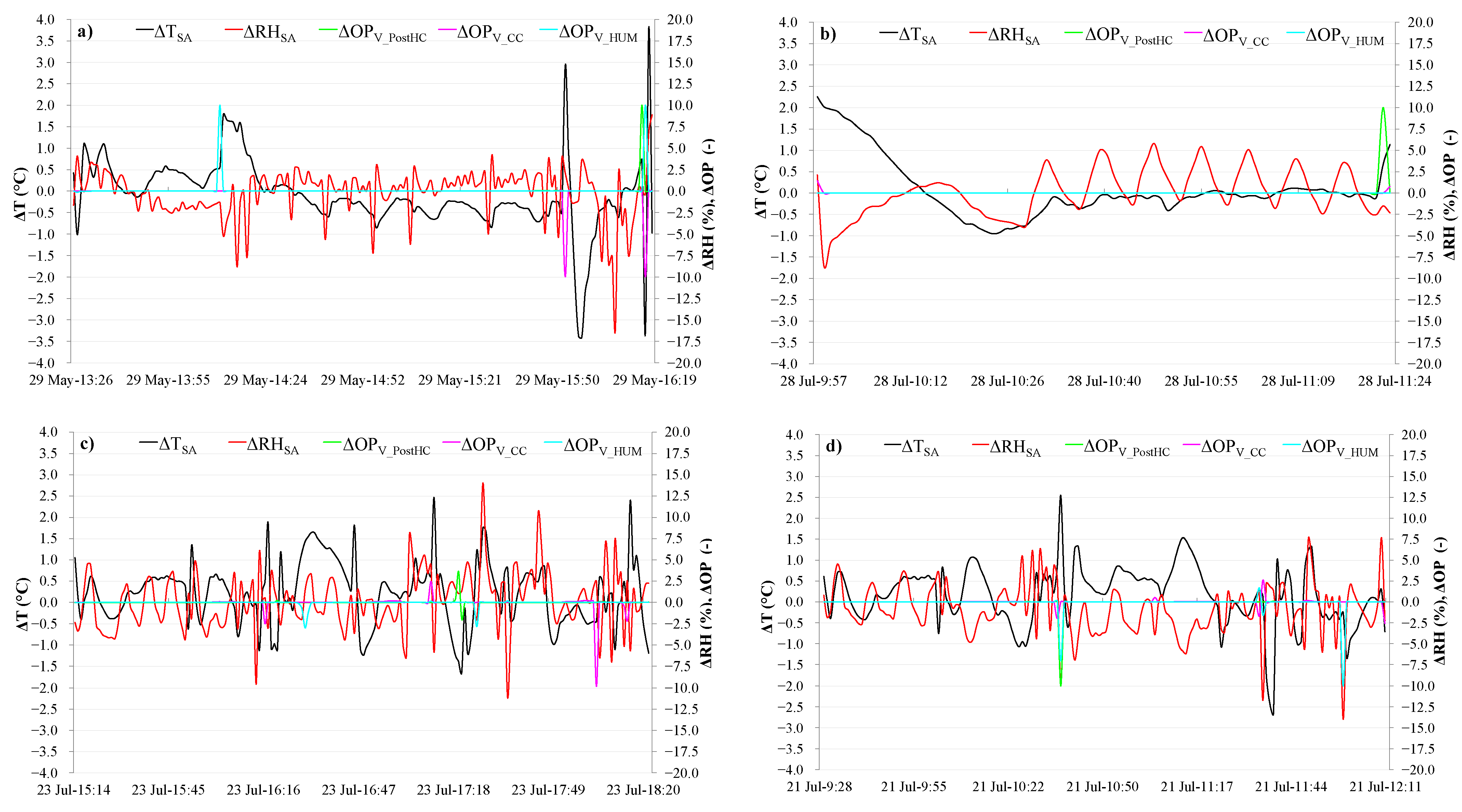
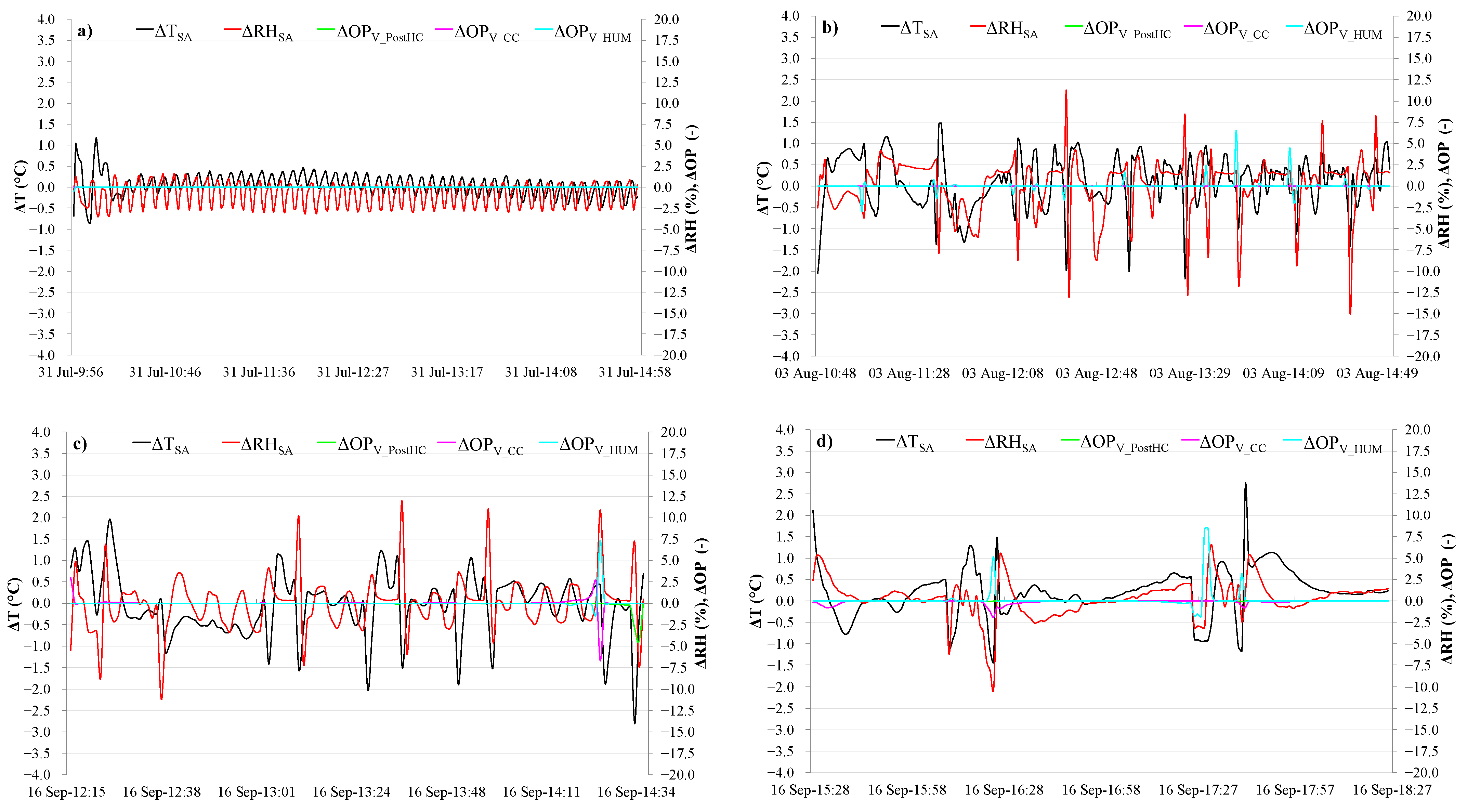
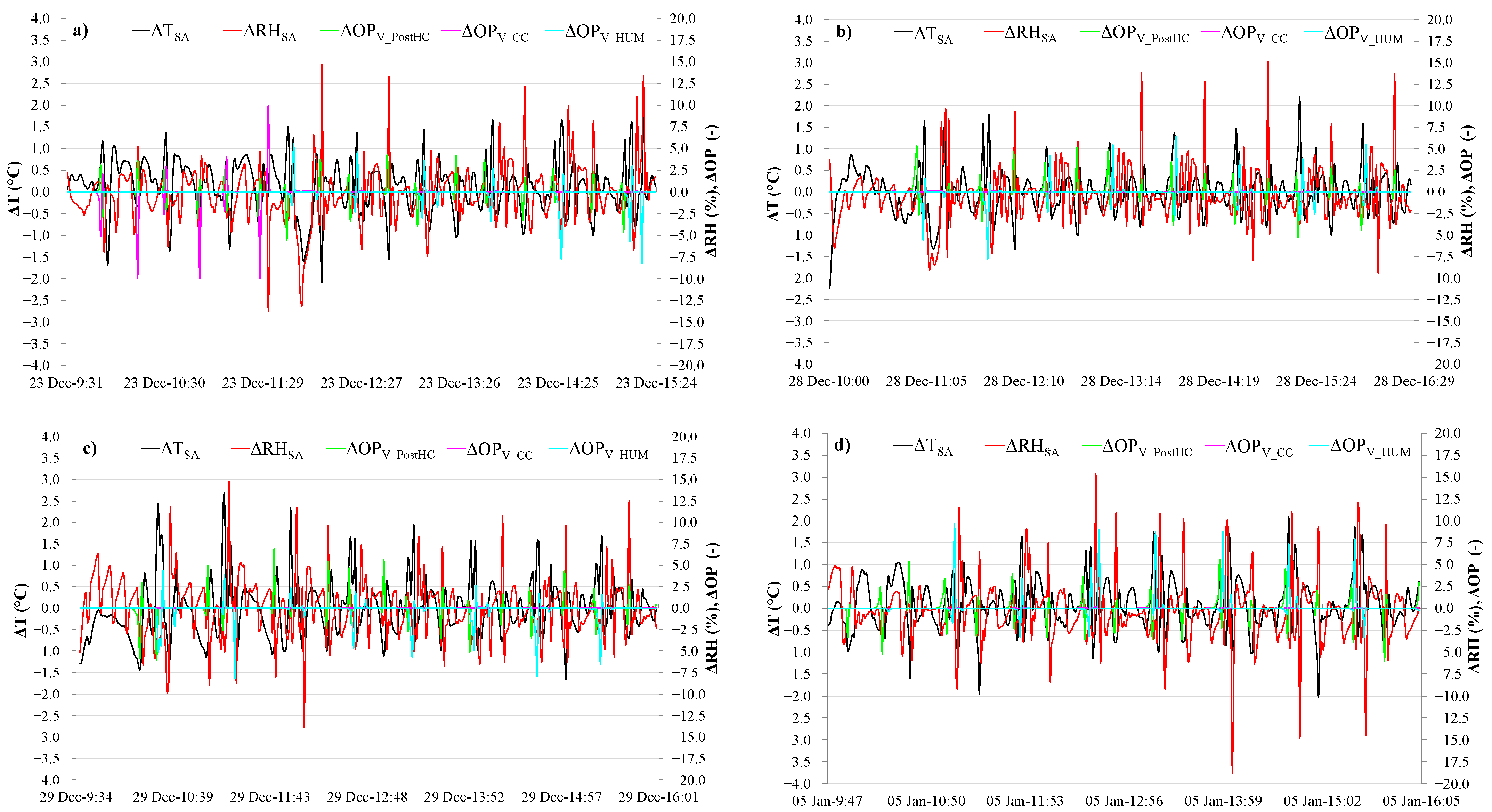
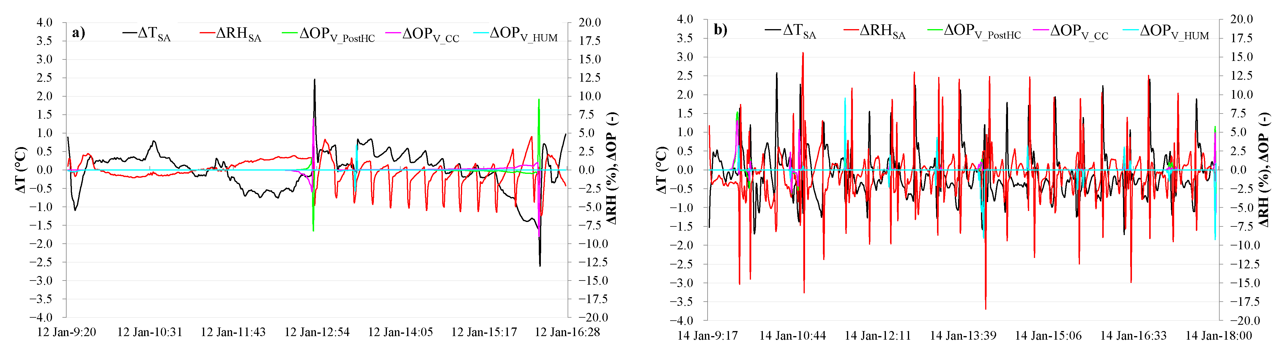
Even if the ANN22 performs better than the ANN16 in predicting the opening percentages of the valves, in this paper the ANN16 has been selected in order to obtain improved predictions in terms of supply air temperature as well as supply air relative humidity (that represent the fundamental outputs of AHU operation), while maintaining an adequate accuracy in forecasting the valves operation. The errors reported in Table 8 demonstrate how the ANN16 can be effectively used to generate operation data for assisting further research in fault detection and diagnosis of HVAC units.

Figure 6, Figure 7, Figure 8 and Figure 9 report the instantaneous errors between the values predicted by the ANN16 and the measured data in terms of (i) supply air temperature (T_SA), (ii) supply air relative humidity (RH_SA), (iii) opening percentage of the post-heating coil valve (OP_{V_PostHC}), (iv) opening percentage of the cooling coil valve (OP_{V_CC}), and (v) opening percentage of the humidifier valve (OP_{V_HUM}) as a function of time.

In more detail, the following parameters are showed in Figure 6, Figure 7, Figure 8 and Figure 9:

$${\mathsf{\Delta }\mathrm{T}}_{\mathrm{SA}}{=\mathrm{T}}_{\mathrm{SA},\mathrm{pred}}{-\mathrm{T}}_{\mathrm{SA},\exp }$$

(7)

$${\mathsf{\Delta }\mathrm{RH}}_{\mathrm{SA}}{=\mathrm{RH}}_{\mathrm{SA},\mathrm{pred}}{-\mathrm{RH}}_{\mathrm{SA},\exp }$$

(8)

$${\mathsf{\Delta }\mathrm{OP}}_{\mathrm{V}\text{\_}\mathrm{PostHC}}{=\mathrm{OP}}_{\mathrm{V}\text{\_}\mathrm{PostHC},\mathrm{pred}}{-\mathrm{OP}}_{\mathrm{V}\text{\_}\mathrm{PostHC},\exp }$$

(9)

$${\mathsf{\Delta }\mathrm{OP}}_{\mathrm{V}\text{\_}\mathrm{CC}}{=\mathrm{OP}}_{\mathrm{V}\text{\_}\mathrm{CC},\mathrm{pred}}{-\mathrm{OP}}_{\mathrm{V}\text{\_}\mathrm{CC},\exp }$$

(10)

$${\mathsf{\Delta }\mathrm{OP}}_{\mathrm{V}\text{\_}\mathrm{HUM}}{=\mathrm{OP}}_{\mathrm{V}\text{\_}\mathrm{HUM},\mathrm{pred}}{-\mathrm{OP}}_{\mathrm{V}\text{\_}\mathrm{HUM},\exp }$$

(11)

where T_{SA, pred}, RH_{SA, pred}, OP_{V_PostHC, pred}, OP_{V_CC, pred}, and OP_{V_HUM, pred} are, respectively, the values predicted by the ANN16, while T_{SA, exp}, RH_{SA, exp}, OP_{V_PostHC, exp}, OP_{V_CC, exp}, and OP_{V_HUM, exp} represent the experimental values.

Figure 6, Figure 7, Figure 8 and Figure 9 highlight that:

• the minimum value of $∆{\mathrm{T}}_{\mathrm{SA}}$ is −3.41 °C (test n. 1), while its maximum value is 3.80 °C (test n. 1);
• the values of $∆{\mathrm{RH}}_{\mathrm{SA}}$ range from −19.20% (test n. 17) up to 17.03% (test n. 17);
• the parameter $∆{\mathrm{OP}}_{\mathrm{V}\text{\_}\mathrm{PostHC}}$ is in the range −10.05% ÷ 10.12%, where the minimum is achieved during the test n. 4, while the maximum refers to the test n. 2;
• the values of $∆{\mathrm{OP}}_{\mathrm{V}\text{\_}\mathrm{CC}}$ vary from −10.03% (test n. 18) up to 10.09% (test n. 9);
• the values of $∆{\mathrm{OP}}_{\mathrm{V}\text{\_}\mathrm{HUM}}$ range between −9.97% (test n. 4) and 10.11% (test n.17).

In order to better point out the results of comparisons between predicted and experimental values reported in Figure 6, Figure 7, Figure 8 and Figure 9, the values of the metrics defined by the Equations (1)–(6), calculated for the parameters specified by the Equations (7)–(11), have been summarized in

Table 9. Errors between the ANN16-based model predictions and experimental points.

		Fault Free Tests during Summer				Faulty Tests during Summer					Fault Free Tests during Winter				Faulty Tests during Winter
Errors	Parameters	Test n. 1	Test n. 2	Test n. 3	Test n. 4	Test n. 5	Test n. 6	Test n. 7	Test n. 8	Test n. 9	Test n. 10	Test n. 11	Test n. 12	Test n. 13	Test n. 14	Test n. 15	Test n. 16	Test n. 17	Test n. 18
$\overline{\mathsf{\epsilon }}$	∆TSA (°C)	−0.10	0.09	0.22	0.17	0.06	0.09	−0.04	0.21	0.01	0.11	−0.01	−0.02	0.07	−0.02	−0.11	0.01	0.22	0.16
	∆RHSA (%)	−0.18	0.04	0.28	−0.88	−0.87	0.11	0.01	0.33	−0.05	−0.24	−0.43	−0.03	−0.36	−0.08	−0.61	−0.22	−0.02	−0.39
	∆OPV_PostHC (%)	0.06	0.11	0.02	−0.06	0.00	−0.01	−0.07	0.00	−0.11	0.01	0.06	0.00	0.02	−0.03	0.05	−0.10	0.00	0.05
	∆OPV_CC (%)	−0.12	0.03	−0.05	−0.01	0.00	0.01	0.03	−0.10	0.06	−0.06	0.02	0.01	0.01	0.02	0.06	0.02	−0.01	−0.31
	∆OPV_HUM (%)	0.12	0.00	−0.04	−0.10	0.00	0.03	0.04	0.12	−0.03	−0.07	−0.03	−0.16	0.11	−0.01	−0.04	0.00	−0.01	−0.16
$\left|\overline{\mathsf{\epsilon }}\right|$	∆TSA (°C)	0.55	0.46	0.60	0.56	0.19	0.38	0.53	0.44	0.43	0.47	0.38	0.48	0.43	0.41	0.47	0.30	0.45	0.46
	∆RHSA (%)	1.97	2.19	2.57	2.40	1.21	11.09	2.12	1.47	1.99	2.24	2.04	2.49	2.32	1.18	2.26	0.70	2.84	1.69
	∆OPV_PostHC (%)	0.06	0.11	0.04	0.06	0.00	0.00	0.07	0.00	0.11	0.24	0.23	0.26	0.30	0.09	0.12	0.10	0.00	0.25
	∆OPV_CC (%)	0.12	0.03	0.11	0.07	0.00	0.00	0.13	0.10	0.07	0.18	0.02	0.01	0.01	0.13	0.12	0.02	0.01	0.36
	∆OPV_HUM (%)	0.12	0.00	0.05	0.13	0.00	0.37	0.07	0.21	0.03	0.19	0.20	0.26	0.22	0.02	0.15	0.00	0.45	0.16
MSE	∆TSA (°C)	0.71	0.51	0.58	0.51	0.07	0.38	0.52	0.36	0.47	0.36	0.27	0.42	0.32	0.28	0.38	0.14	0.34	0.32
	∆RHSA (%)	8.59	7.44	11.13	10.23	2.48	11.09	10.08	4.85	6.15	10.50	9.12	11.06	12.27	2.73	13.25	1.08	22.41	5.19
	∆OPV_PostHC (%)	0.58	1.15	0.09	0.62	0.00	0.00	0.22	0.00	1.18	0.74	0.73	0.99	0.95	0.40	0.43	0.31	0.00	0.87
	∆OPV_CC (%)	1.16	0.03	0.60	0.13	0.00	0.00	0.47	0.07	0.60	1.33	0.00	0.00	0.00	0.38	0.40	0.00	0.00	3.00
	∆OPV_HUM (%)	1.16	0.00	0.10	0.95	0.00	0.37	0.42	1.12	0.03	0.85	0.79	1.10	1.38	0.05	0.78	0.00	2.63	0.29
RMSE	∆TSA (°C)	0.84	0.71	0.73	0.70	0.25	0.61	0.72	0.57	0.67	0.59	0.52	0.65	0.56	0.53	0.61	0.37	0.54	0.54
	∆RHSA (%)	2.93	2.74	3.34	3.09	1.32	3.34	3.19	2.18	2.42	3.24	2.99	3.33	3.49	1.65	3.59	1.02	4.74	2.25
	∆OPV_PostHC (%)	0.76	1.07	0.30	0.79	0.00	0.01	0.46	0.01	1.05	0.86	0.85	1.00	0.98	0.63	0.65	0.55	0.01	0.93
	∆OPV_CC (%)	1.08	0.17	0.78	0.35	0.00	0.01	0.68	0.25	0.75	1.15	0.03	0.02	0.02	0.61	0.63	0.04	0.07	1.71
	∆OPV_HUM (%)	1.07	0.00	0.32	0.97	0.03	0.61	0.65	1.05	0.17	0.92	0.89	1.04	1.17	0.21	0.89	0.01	1.62	0.51
R2	∆TSA (°C)	0.98	0.99	0.99	0.99	0.98	0.85	0.96	0.92	0.99	0.99	0.99	0.99	0.99	1.00	0.99	0.60	0.85	0.99
	∆RHSA (%)	0.97	0.76	0.97	0.96	0.89	0.92	0.93	0.94	0.96	0.97	0.98	0.97	0.97	1.00	0.97	0.77	0.87	0.98
	∆OPV_PostHC (%)	0.95	0.49	1.00	0.98	1.00	1.00	1.00	1.00	1.00	0.97	0.97	0.96	0.96	0.98	0.89	1.00	1.00	0.96
	∆OPV_CC (%)	0.91	1.00	0.95	0.99	1.00	1.00	0.97	1.00	1.00	0.91	1.00	1.00	1.00	0.98	0.90	1.00	1.00	0.88
	∆OPV_HUM (%)	0.94	1.00	0.99	0.94	1.00	0.98	0.98	0.92	1.00	0.93	0.95	0.92	0.86	1.00	0.94	1.00	0.87	1.00

. For each line of this table, the green shade has been assigned to the cells corresponding to the best performance, while the worst results have been highlighted by red shades.

This table underlines that the ANN16 is able to carefully predict the experimental data measured during summer and winter under both normal and faulty conditions and it provides a rigorous representation of the HVAC system’s steady-state and transient operation taking into account that:

• with reference to all the tests, the average values of R² in predicting T_SA, RH_SA, OP_{V_PostHC}, OP_{V_CC} and OP_{V_HUM} are, respectively, 0.95 °C, 0.93%, 0.95%, 0.97%, and 0.96%;
• with reference to the tests n. 1–4 (performed without faults during summer), the values of R² are always larger than 0.9 for all the parameters, except the cases of ∆RH_SA and ∆OP_{V_PostHC} for the test n. 2;
• with reference to the tests n. 5–9 (performed with faults during summer), the coefficient of determination is always greater than 0.9 for all the parameters, except the cases of ∆RH_SA for the test n. 5 (with fault 1) and ∆T_SA for the test n. 6 (with fault 2);
• with reference to the tests n. 10–13 (performed without faults during winter), the values of R² are always larger than 0.9 for all the parameters, except the case of ∆OP_{V_HUM} for the test n. 13;
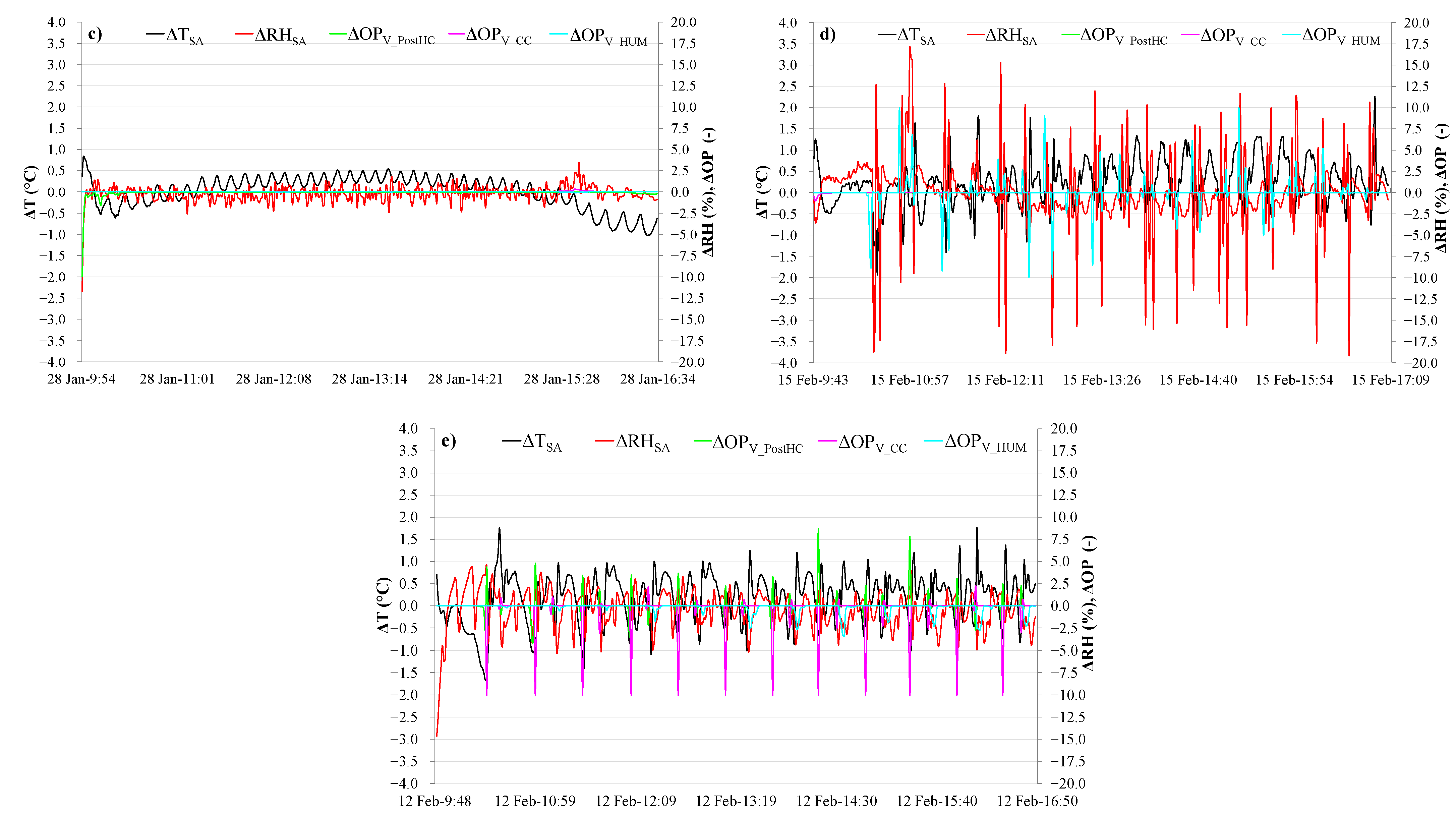
• with reference to the tests n. 14–18 (performed with faults during winter), the coefficient of determination is always greater than 0.9 for all the parameters, except (i) the cases of both ∆T_SA and ∆RH_SA for both the tests n. 16 (fault 3) and n. 17 (fault 4), (ii) the cases of both ∆OP_{V_PostHC} and ∆OP_{V_CC} for the test n. 15 (fault 2), (iii) the case of ∆OP_{V_CC} for the test n. 18 (fault 5) as well as (iv) the case of ∆OP_HUM for the test n. 17 (fault 4);
• whatever the test is, the values of $\left|\overline{\mathsf{\epsilon }}\right|$ for the parameter ∆T_SA are always lower than 0.8 °C (that is the accuracy of the sensor used for measuring T_SA), with a minimum of 0.19 °C (test n. 5) up to a maximum of 0.60 °C (test. n. 3);
• the values of $\left|\overline{\mathsf{\epsilon }}\right|$ for the parameter ∆RH_SA range between a minimum of 0.7% up to a maximum of 11.1% and, therefore, they are always smaller than 3% (that is the accuracy of the sensor used for measuring RH_SA), except the only case of the test n. 6 (performed with fault 2 during summer);
• the maximum values of MSE and RMSE with reference to the parameter ∆T_SA are, respectively, not larger than 0.71 °C and 0.84 °C (obtained for the test n. 1 performed without faults during summer);
• the maximum values of MSE and RMSE with reference to the parameter ∆RH_SA are, respectively, not larger than 22.4% and 4.74% (achieved for the test n. 17 performed with fault 4 during winter);
• the maximum value of MSE with reference to the parameters ∆OP_{V_PostHC}, ∆OP_{V_CC} and ∆OP_{V_HUM} is 3.0%, obtained in the case of the test n. 18 performed with fault 5 during winter;
• the maximum value of RMSE with reference to the parameters ∆OP_{V_PostHC}, ∆OP_{V_CC} and ∆OP_{V_HUM} is 1.7%, achieved in the case of the test n. 18 performed with fault 5 during winter.

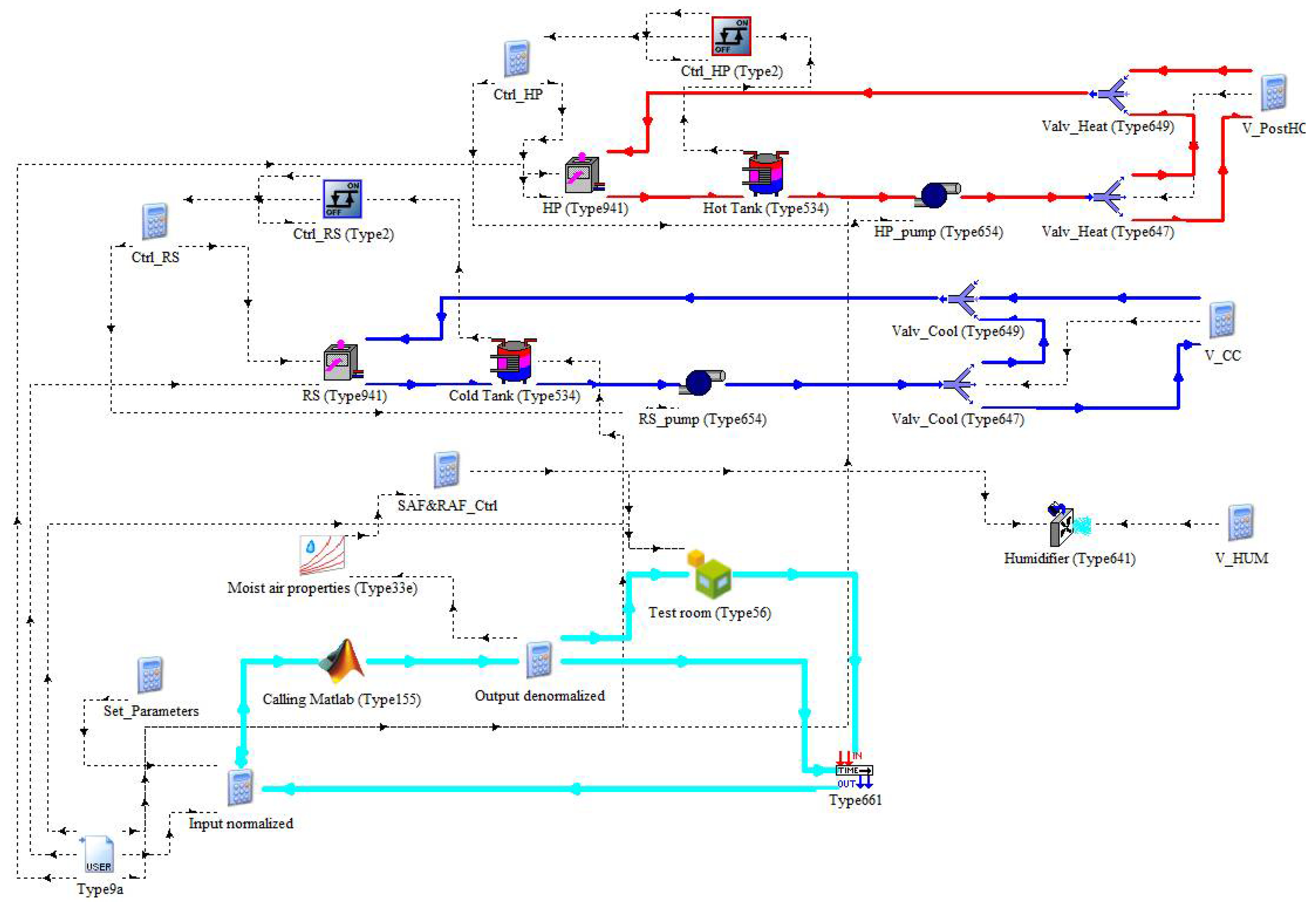
4.2. TRNSYS Model

In the dynamic simulation software TRNSYS (version 17) [33], the whole system is first broken up into specific models (named “Types”) of each single system component, where each “Type” is represented by a FORTRAN code. The users can assemble the TRNSYS Types by connecting component outputs with component inputs and then specifying the corresponding components’ performance parameters. Finally, the software solves the corresponding equations in order to characterize the component/system operation every time step.

In this study, a detailed model in TRNSYS environment has been developed to simulate, using a time step of 1 min (according to the time step of experimental data utilized in this work for training, testing, and validating the ANN-based model), (i) the return air temperature (T_RA); (ii) the return air relative humidity (RH_RA); as well as the electric energy consumptions (not measured) of (iii) the heat pump (HP), (iv) the refrigerating system (RS), (v) the humidifier (HUM), (vi) the supply air fan (SAF), and (vii) the return air fan (RAF). With reference to the several performance parameters to be specified in the TRNSYS Types used into the simulation model, it can be noticed that, in this study, some of the parameters have been directly identified or calculated based on catalog data; the remaining parameters have been defined based on field measurements.

Table 10. Main simulated components and corresponding types of TRNSYS software.

Simulated Component	TRNSYS Type/Model
Test room	56
Heat pump/Refrigerating system	941
Hot and cold tanks	534
Humidifier	641
HP/RS pump	654
Diverting/mixing valves	647/649
On/Off differential controllers	2
Moist air properties	33e
Integrated test room	56

lists the main modeled components and the corresponding TRNSYS Types used in the simulation model.

Figure 10 depicts a screenshot of the TRNSYS model, highlighting the main circuits with different colors. In particular, the circuit of cold fluid supplied by the refrigerating system to the cooling coil is depicted in blue; the circuit of hot fluid supplied by the heat pump to the post-heating coil is indicated in red; finally, the inputs and outputs of the ANN-based model are highlighted in light blue. The other connections of TRNSYS Types are pointed out by dashed black lines.

The TRNSYS model has been coupled with the artificial neural network ANN16 (described in the previous section) via the TRNSYS Type 155.

The ANN16 uses as inputs the 10 variables indicated in the previous section and provides as outputs the 5 parameters specified in the same section.

The Type 155 links ANN16 with both the Type 56 as well as the Type 661. In particular, the Type 155 provides two of the outputs of the ANN16, i.e., the supply air temperature and relative humidity, as inputs to the Type 56. In addition, the Type 155 provides as inputs to the Type 661 all the outputs of the ANN16, i.e., the supply air temperature, the supply air relative humidity, as well as the opening percentages of the valves supplying the humidifier, the pre-heating coil, and the cooling coil. The Type 661 models a “sticky” controller with its outputs assumed equal to the inputs at the earlier time step; the outputs of the Type 661 are then provided as inputs to the Type 155.

A dynamic model of the “building” corresponding to the integrated test room has been developed by means of the Type 56. This model allows calculation of the return air temperature and relative humidity (then assigned as inputs to the Type 661) according to the geometry, thermo-physical properties of walls’ layers, air infiltration rate, as well as internal loads/gains. In particular, the geometry and walls’ layers have been characterized according to the content of the previous section, while air infiltration rate as well as internal loads/gains are kept equal to zero according to the experimental conditions.

The Type 941 has been considered for simulating the operation of both the refrigerating unit (RS) and the heat pump (HP) of the experimental setup. This Type allows to obtain as outputs (a) the absorbed power and (b) the exiting fluid temperature in the case of (i) the outside air temperature, (ii) the entering fluid temperature, (iii) the fluid flow rate, as well as (iv) the performance maps of the devices are provided as inputs. In this study, the outside temperature has been assumed to be equal to the measured values (the Type 9a has been used for reading data from an external file and making them available to the TRNSYS Types 941), the fluid mass flow rate is set to 2310 kg/h for the refrigerating system and 2410 kg/h for the heat pump according to the manufacturer datasheet [36], and the performance maps suggested by the manufacturer [36] and reported in Figure A2a,b of Appendix A have been provided. In particular, Figure A2a,b, respectively, indicates the coefficient of performance COP of the heap pump (useful thermal power output divided by required electric power input) and the energy efficiency ratio EER of the refrigerating system (useful cooling power output divided by required electric power input) depending on supply fluid temperature and outside air temperature.

Both the heat pump and the refrigerating system are coupled with a 75 L tank that is devoted to storing the hot and cold fluids, respectively. The operations of both hot and cold tanks have been simulated with the Type 534. This Type models a cylindrical vertical tank; it divides the tanks into 10 isothermal temperature layers in order to carefully consider thermal stratification (where the layer n. 1 is positioned on the uppermost portion of the tank and the layer n. 10 is positioned on the lowest part of the tank).

With reference to the modeling of the fans, a specifically devoted data set was gathered from a calibration activity performed by adjusting and maintaining the supply and return fans at various speeds from 10% to 100%. Figure A3 in Appendix A shows the air volumetric flow rate Q_V measured at SENS i-Lab and the power consumption P_el suggested by the manufacturer as a function of the fan’ velocity OL. In particular, Figure A3a refers to the supply air fan, while Figure A3b is related to the return air fan.

The following equations, interpolating the values reported in Figure A3a,b, have been derived to calculate both the air volumetric flow rate Q_V as well as the power consumption P_el of both supply and return air fans as a function of fans’ velocity:

Q_V^SAF = −0.00001∙OL_SAF³ + 0.0634∙OL_SAF² + 5.1789∙OL_SAF + 8.7704

(12)

P_el^SAF = 0.0003∙OL_SAF³ + 0.1068∙OL_SAF² + 0.7383∙OL_SAF + 4.9372

(13)

Q_V^RAF = 14.491∙ OL_RAF + 12.352

(14)

P_el^RAF = 0.001∙OL_RAF³ – 0.078∙OL_RAF² + 3.120∙OL_RAF − 2.102

(15)

Equations (12)–(15) have been included in the TRNSYS project via the Type 9a (external file data reader) for calculating the fans’ power consumption according to the fans’ velocity.

The operation of the adiabatic steam humidifier has been modeled via the Type 641; this model permits the humidifier not to respond instantaneously to the control signal, but to get the steady-state values of both power consumption and gain rate exponentially. In the TRNSYS project, the control signal associated to the opening percentage of the humidifier valve is provided as input to the Type 641 by the ANN16 through the Type 155. Based on catalog data, the humidifier power consumption has been considered equal to the nominal value of 3.7 kW, while the humidifier is activated taking into account that it has been experimentally verified that water flow rate supplied by the humidifier increases from the minimum to the maximum value (5 kg/h) almost instantaneously.

The Type 654 has been used for modeling the single-speed pumps maintaining a constant fluid flow exiting/entering the heat pump and the refrigerating system.

The Type 647 has been used to model the diverting valves that split a liquid inlet flow into two fractional outlet flows, while the Type 649 is adopted to simulate the mixing valves that combine two individual liquid streams into a single outlet.

The moist air properties have been evaluated by means of the Type 33e; this Type takes as inputs the air relative humidity and the air dry bulb temperature and generate the other corresponding air properties as outputs.

In this paper, the Type 2 has been adopted for simulating on/off differential controllers. These devises generate a value in the range between 0 and 1 that is used to deactivate or activate the refrigerating system or the heat pump. In particular, this Type activates the component generating a signal equal to 1 when the observed parameter becomes lower than the user-defined setpoint by a certain value (upper deadband), while it is switched off in the case of the observed parameter approaches the user-defined setpoint within a given limit (lower deadband). The successive value generated by the differential controller is also affected by the value assumed by the control signal used as input at the earlier time step. In this work, the differential controller is operated by connecting the input and output signals in order to give a hysteresis effect. In greater detail, the temperature at node 2 of the tank storing the cold fluid has been assumed as the observed temperature for activating/deactivating the refrigeration unit; with reference to the hot tank, the temperature at node 8 has been adopted as the watched temperature for operating the heat pump. A target temperature of 45 °C was assumed for activating the heap pump, with a turn-on temperature difference of 1 °C and a turn-off temperature difference of −1 °C. A target temperature of 7 °C was defined for activating the refrigeration unit, with a turn-on temperature difference of 1 °C and a turn-off temperature difference of −1 °C. The hot/cold heat carrier fluid is moved by the pumps into the post-heating/cooling coil according to the opening percentage of the corresponding valves defined by the related outputs of the ANN16 via the Type 155. The temperature of the hot heat carrier fluid is assumed to be reduced by 5 °C when flowing into the post-heating coil (before entering the hot tank), while the temperature of the cold heat carrier fluid is assumed as increased by 5 °C when flowing into the cooling coil (before entering the cold tank).

5. Assessment of Faults’ Impact

In this section, the experimental performances of the HVAC system operating under faulty conditions (summer tests n. 5–9 of Table 4 and winter tests n. 14–18 of Table 5) have been compared with those predicted by the artificial neural network ANN16 (described in Section 4a), coupled with the TRNSYS model (described in Section 4b), in the cases of the HVAC system is operating under the same boundary conditions without faults. In more detail, the following inputs have been provided to the ANN16 in order to simulate the HVAC performance without faults: (i) return air temperature calculated by the TRNSYS Type 56 as well as target of indoor air temperature equal to 26 °C; (ii) return air relative humidity calculated by the TRNSYS Type 56 as well as target of indoor air relative humidity equal to 50%; (iii) supply air temperature calculated by the ANN16 itself at previous time step; (iv) supply air relative humidity calculated by the ANN16 itself at previous time step; (v) experimental value of outside air temperature; (vi) opening percentage of the valve supplying the post-heating coil calculated by the ANN16 itself at previous time step; (vii) opening percentage of the valve supplying the cooling coil calculated by the ANN16 itself at previous time step; (viii) opening percentage of the valve supplying the humidifier calculated by the ANN16 itself at previous time step; (ix) velocity of supply air fan equal to the nominal value of 50%; and (x) velocity of return air fan equal to the nominal value of 50%.This means that:

• The experimental tests n. 5 and n. 14 (with the fault 1, i.e., with the velocity of the supply air fan kept at 20%) have been compared with the simulation cases where the velocity of supply air fan has been kept at the nominal value of 50%;
• The experimental tests n. 6 and n. 15 (with the fault 2, i.e., the velocity of the return air fan kept at 20%) have been compared with the simulation cases where the velocity of return air fan has been kept at the nominal value of 50%;
• The experimental tests n. 7 and n. 16 (with the fault 3, i.e., the post-heating coil valve kept always closed) have been compared with the simulation cases where the values of OP_{V_PostHC} can vary according to the automatic control logic in the range of 0 to 100;
• The experimental tests n. 8 and n. 17 (with the fault 4, i.e., the cooling coil valve kept always closed) have been compared with the simulation cases where the values of OP_{V_CC} can vary according to the automatic control logic in the range of 0 to 100;
• The experimental tests n. 9 and n. 18 (with the fault 5, i.e., the opening percentage of the steam humidifier valve kept always closed) have been compared with the simulation cases where the values of OP_{V_HUM} can vary according to the automatic control logic in the range of 0 to 100.

Figure 11 and Figure 12 highlight the values of return air temperature (T_RA) and return air relative humidity (RH_RA) over time, for the cases without faults (predicted values represented by solid lines) and the cases when only one of the 5 above-mentioned faults is occurred (experimental values indicated by dashed lines) with the aim of helping the contrast between normal and faulty scenarios. In particular, Figure 11 refers to the summer tests, while Figure 12 corresponds to the winter tests.

These comparisons have been performed in order to assess the impact of each fault on (i) the capability to achieve the desired indoor conditions, (ii) the arithmetic mean and standard deviation of return air temperature and relative humidity, as well as (iii) the electric energy consumptions. In particular, the effects of faults on occupant thermo-hygrometric comfort are reported in Section 5.1.; the faults’ impact associated with the trends of return air temperature and relative humidity is described in Section 5.2.; the influence of each fault on electric energy consumptions is indicated in Section 5.3. The discussion about all the results is performed in last Section 5.4.

5.1. Results: Faults’ Impact on Thermo-Hygrometric Comfort

Table 11. Thermal-hygrometric time with/without faults.

	ID Test		Thermal Comfort Time (%)	Hygrometric Comfort Time (%)
Summer tests	Test 5	With fault 1 (experimental)	0.00	16.17
		Without fault (predicted)	65.79	86.84
		Difference between faulty and healthy operation	−65.79	−70.67
	Test 6	With fault 2 (experimental)	50.61	81.38
		Without fault (predicted)	58.70	88.26
		Difference between faulty and healthy operation	−8.09	−6.88
	Test 7	With fault 3 (experimental)	13.43	88.06
		Without fault (predicted)	81.95	88.72
		Difference between faulty and healthy operation	−68.52	−0.66
	Test 8	With fault 4 (experimental)	0.00	90.59
		Without fault (predicted)	63.31	94.67
		Difference between faulty and healthy operation	−63.31	−4.08
	Test 9	With fault 5 (experimental)	86.59	65.36
		Without fault (predicted)	84.00	81.14
		Difference between faulty and healthy operation	2.59	−15.78
Winter tests	Test 14	With fault 1 (experimental)	75.41	49.41
		Without fault (predicted)	76.11	87.35
		Difference between faulty and healthy operation	−0.70	−37.94
	Test 15	With fault 2 (experimental)	68.71	82.34
		Without fault (predicted)	69.23	86.23
		Difference between faulty and healthy operation	−0.52	−3.89
	Test 16	With fault 3 (experimental)	0.00	99.75
		Without fault (predicted)	69.75	86.25
		Difference between faulty and healthy operation	−69.75	13.50
	Test 17	With fault 4 (experimental)	15.73	80.45
		Without fault (predicted)	67.79	95.72
		Difference between faulty and healthy operation	−52.06	−15.27
	Test 18	With fault 5 (experimental)	64.85	22.67
		Without fault (predicted)	70.48	51.03
		Difference between faulty and healthy operation	−5.63	−28.36

compares the thermal/hygrometric comfort times (i.e., the percentage of time during with values of indoor air temperature/relative humidity within the given deadbands) of the simulation tests without faults with respect to those associated to the corresponding experimental tests when only one of the five faults (described in the previous Section 3) is occurring.

5.2. Results: Faults’ Impact on Key Operating Parameters

Experimental data under faulty operation and predicted data under fault-free operation were compared by calculating the arithmetic mean μ and the standard deviation σ of (1) return air temperature (T_RA) and (2) return air relative humidity (RH_RA). The arithmetic mean μ and standard deviation σ have been calculated by means of the following formulas:

$$\mathsf{\mu }={\displaystyle \sum _{\mathrm{i}=1}^{\mathrm{N}}\frac{{\mathrm{d}}_{\mathrm{i}}}{\mathrm{N}}}$$

(16)

$$\mathsf{\sigma }=\sqrt{\frac{{\displaystyle \sum _{\mathrm{i}=1}^{\mathrm{N}}{\left({\mathrm{d}}_{\mathrm{i}}-\mathsf{\mu }\right)}^2}}{\mathrm{N}}}$$

(17)

where N is the whole number of points, while d_i is the value at time step i of the above-mentioned parameters.

Table 12. Differences between predicted fault free data and experimental faulty data in terms of T_RA and RH_RA.

	ID Test		TRA (°C)		RHRA (%)
			μ	σ	μ	σ
Summer tests	Test 5	With fault 1 (experimental)	28.55	0.22	56.17	1.54
		Without fault (predicted)	26.20	1.28	48.58	3.36
		%D	8.98%	−82.73%	15.64%	−54.25%
	Test 6	With fault 2 (experimental)	27.72	1.78	49.32	3.59
		Without fault (predicted)	27.16	1.79	49.97	3.30
		%D	2.07%	−0.17%	−1.30%	8.75%
	Test 7	With fault 3 (experimental)	24.72	1.20	48.88	3.56
		Without fault (predicted)	26.12	0.84	48.42	3.22
		%D	−5.34%	42.68%	0.96%	10.46%
	Test 8	With fault 4 (experimental)	28.50	0.14	47.77	3.06
		Without fault (predicted)	26.57	1.28	50.13	2.92
		%D	7.24%	−89.05%	−4.69%	4.93%
	Test 9	With fault 5 (experimental)	25.88	0.74	47.50	3.31
		Without fault (predicted)	25.95	0.77	51.15	3.71
		%D	−0.27%	−3.48%	−7.14%	−10.79%
Winter tests	Test 14	With fault 1 (experimental)	19.77	0.80	45.18	1.48
		Without fault (predicted)	20.14	0.84	49.61	3.38
		%D	−1.85%	−4.26%	−8.93%	−56.06%
	Test 15	With fault 2 (experimental)	20.18	0.86	50.12	4.01
		Without fault (predicted)	20.21	0.88	49.70	3.42
		%D	−0.13%	−1.35%	0.85%	17.23%
	Test 16	With fault 3 (experimental)	15.71	0.69	47.22	0.91
		Without fault (predicted)	20.21	0.87	49.67	3.41
		%D	−22.25%	−20.88%	−4.94%	−73.38%
	Test 17	With fault 4 (experimental)	21.55	0.59	49.99	3.95
		Without fault (predicted)	20.38	1.06	50.48	2.76
		%D	5.77%	−44.25%	−0.98%	43.17%
	Test 18	With fault 5 (experimental)	20.30	0.97	47.05	2.41
		Without fault (predicted)	20.25	0.89	49.56	3.46
		%D	0.25%	9.53%	−5.07%	−30.29%

compares the arithmetic mean μ and standard deviation σ during tests 5–9 (summer tests) and 14–18 (winter tests).

Table 12 also shows the percentage difference (%D) between the values of arithmetic mean and the standard deviation under faulty (predicted values) and fault free operation (experimental values) for each of the above-mentioned parameters. The percentage difference %D has been calculated by means of the following formula:

$$\%\mathrm{D}=\frac{\left({\mathrm{X}}_{\mathrm{fault},\mathrm{i}}{-\mathrm{X}}_{\mathrm{w}/\mathrm{o}\text{\_}\mathrm{fault},\mathrm{i}}\right)}{{\mathrm{X}}_{\mathrm{w}/\mathrm{o}\text{\_}\mathrm{fault},\mathrm{i}}}\times 100$$

(18)

where X is the arithmetic mean μ or the standard deviation σ of T_RA or RH_RA.

Table 13. Summary of symptoms associated to the 5 typical faults on T_RA and RH_RA.

	ID Fault	TRA		RHRA
		μ	σ	μ	σ
Summer tests	Fault 1 (related to velocity of the supply air fan)	0	-	0	-
	Fault 2 (related to velocity of the return air fan)	0	0	0	0
	Fault 3 (related to the post-heating coil valve)	0	+	0	0
	Fault 4 (related to the cooling coil valve)	0	-	0	0
	Fault 5 (related to the humidifier valve)	0	0	0	0
Winter tests	Fault 1 (related to velocity of the supply air fan)	0	0	0	-
	Fault 2 (related to velocity of the return air fan)	0	0	0	0
	Fault 3 (related to the post-heating coil valve)	-	-	0	-
	Fault 4 (related to the cooling coil valve)	0	-	0	+
	Fault 5 (related to the humidifier valve)	0	0	0	-

summarizes the comments described above; for each of five typical faults considered and for each of four parameters, a performance index has been assigned with the following signs: “+” indicates that the fault causes substantial positive changes (greater than 20%) of %D; “-” indicates that the fault causes substantial negative changes (greater than −20%) of %D; “0” indicates that the fault causes not substantial changes (between −20% and 20%) of %D.

5.3. Results: Faults’ Impact on Electric Energy Consumption

Table 14. Electric energy consumption with and without faults.

	ID Test		Electric Energy Consumption
			EEHP (kWh)	EERS (kWh)	EEHUM (kWh)	EESAF (kWh)	EERAF (kWh)	EETOT (kWh)
Summer tests	Test 5	With fault 1 (experimental)	0.28	19.37	0.00	0.17	0.43	20.25
		Without fault (predicted)	9.43	18.99	4.75	1.29	0.43	34.89
		EPD	+97%	−2%	+100%	+87%	0%	+42%
	Test 6	With fault 2 (experimental)	0.29	16.68	9.00	1.04	0.12	27.13
		Without fault (predicted)	5.45	13.88	7.09	1.04	0.35	27.81
		EPD	+95%	−20%	−27%	0%	+66%	+2%
	Test 7	With fault 3 (experimental)	0.22	7.19	2.65	0.56	0.19	10.81
		Without fault (predicted)	4.35	6.91	2.34	0.56	0.19	14.35
		EPD	+95%	−4%	−13%	0%	0%	+25%
	Test 8	With fault 4 (experimental)	0.22	0.99	1.48	0.72	0.24	3.65
		Without fault (predicted)	4.94	10.13	2.96	0.72	0.24	18.99
		EPD	+96%	+90%	+50%	0%	0%	+81%
	Test 9	With fault 5 (experimental)	2.65	8.76	0.00	0.74	0.25	12.40
		Without fault (predicted)	3.90	10.94	3.88	0.74	0.25	19.71
		EPD	+32%	+20%	+100%	0%	0%	+37%
Winter tests	Test 14	With fault 1 (experimental)	13.13	8.49	11.04	0.17	0.61	33.44
		Without fault (predicted)	16.30	13.56	16.16	1.81	0.61	48.44
		EPD	+19%	+37%	+32%	+91%	0%	+31%
	Test 15	With fault 2 (experimental)	28.95	20.23	17.70	2.21	0.25	69.34
		Without fault (predicted)	20.90	21.01	19.36	2.21	0.74	64.22
		EPD	−39%	+4%	+9%	0%	+66%	−8%
	Test 16	With fault 3 (experimental)	0.61	16.27	0.00	1.70	0.57	19.15
		Without fault (predicted)	16.37	12.26	14.00	1.70	0.57	44.90
		EPD	+96%	−33%	+100%	0%	0%	+57%
	Test 17	With fault 4 (experimental)	0.61	0.37	7.65	1.89	0.63	11.15
		Without fault (predicted)	14.85	18.06	9.31	1.89	0.63	44.74
		EPD	+96%	+98%	+18%	0%	0%	+75%
	Test 18	With fault 5 (experimental)	9.05	11.24	0.00	1.78	0.60	22.67
		Without fault (predicted)	16.20	17.10	15.35	1.78	0.60	51.03
		EPD	+44%	+34%	+100%	0%	0%	+56%

shows the electric energy consumptions of: the heat pump (EE_HP), the refrigerating system (EE_RS), the humidifier (EE_HUM), the supply air fan (EE_SAF), the return air fan (EE_RAF), and the total electric energy consumption (EE_TOT), with and without faults; in particular, the values associated to the faulty tests have been derived as outputs of the TRNSYS model by using the measured data as inputs, while the values associated to the fault free tests have been predicted by the coupling of the ANN16 and the TRNSYS model. Moreover, Table 14 reports the energy percentage difference (EPD) that has been valuated as follows:

$$\mathrm{EPD}=\frac{{\mathrm{EE}}_{\mathrm{w}/\mathrm{o}\text{\_}\mathrm{fault},\mathrm{i}}{-\mathrm{EE}}_{\mathrm{fault},\mathrm{i}}}{{\mathrm{EE}}_{\mathrm{w}/\mathrm{o}\text{\_}\mathrm{fault},\mathrm{i}}}\times 100$$

(19)

where EE_{w/o_fault,i} and EE_fault,i are, respectively, the electric energy consumption of AHU component for the case without faults and with one of the above-mentioned faults.

5.4. Discussion

With respect to the case without faults, Table 11 and Table 14 indicate the effects of the occurrence of fault 1 (velocity of supply air fan kept reduced at 20% instead of the nominal value of 50%):

• During summer (test n. 5) it strongly reduces both the thermal comfort time (66%) and the hygrometric comfort time (71%), while significantly lowering the overall electric energy consumption (42%) thanks to reduced consumption of the heat pump (97%), the steam humidifier (100%), and the supply air fan (87%);
• During winter (test n. 14) it decreases the hygrometric comfort time (38%), without significant variation of the hygrometric comfort time (1%), while considerably lowering the total electric energy consumption (31%) thanks to reduced consumption of the refrigerating system (37%), the heat pump (19%), the steam humidifier (32%), and the supply air fan (91%).

With respect to the case without fault, Table 11 and Table 14 demonstrate the effects of the occurrence of fault 2 (velocity of return air fan kept reduced at 20% instead of the nominal value of 50%):

• During summer (test n. 6) slightly decreases both the thermal comfort time (8%) and the hygrometric comfort time (7%), while slightly reducing the overall electric energy consumption (2%) because of the lower consumption of both the heat pump (95%) and return air fan (66%);
• During winter (test n. 15) slightly decreases the hygrometric comfort time (4%), without relevant variation of the hygrometric comfort time (1%), while increasing the overall electric energy consumption (8%) due to greater consumption of heat pump (39%).

With respect to the case without fault, Table 11 and Table 14 show how the occurrence of the fault 3 (the opening percentage of the valve regulating the flow to the post-hating coil kept closed instead of allowing its normal operation in the range of 0 to 100 according to the automatic control logic):

• During summer (test n. 7) strongly reduces the thermal comfort time (69%), without significant variation of the hygrometric comfort time (1%), while lowering the overall electric energy consumption (25%) because of the reduced consumption of the heat pump (95%);
• During winter (test n. 16) strongly reduces the thermal comfort time (70%) and slightly decreases the hygrometric comfort time (14%), while significantly lowering the overall electric energy consumption (57%) because of the reduced consumption of both the heat pump (96%), and the steam humidifier (100%).

With respect to the case without fault, Table 11 and Table 14 highlight how the occurrence of the fault 4 (the opening percentage of the valve regulating the flow to the cooling coil kept closed instead of allowing its normal operation in the range of 0 to 100 according to the automatic control logic):

• During summer (test 8) significantly decreases the thermal comfort time (63%) and slightly reduces the hygrometric comfort time (4%), while greatly lowering the overall electric energy demand (81%) because of the reduced consumption of the heat pump (96%), the refrigerating system (90%), and the steam humidifier (50%);
• During winter (test n. 17) significantly decreases the thermal comfort time (52%) and slightly reduces the hygrometric comfort time (15%), while considerably lowering the overall electric energy demand (75%) because of the reduced consumption of the heat pump (96%), the refrigerating system (98%), and the steam humidifier (18%).

With respect to the case without fault, Table 11 and Table 14 indicate how the occurrence of the fault 5 (the opening percentage of the valve regulating the flow to the steam humidifier kept closed instead of allowing its normal operation in the range of 0 to 100 according to the automatic control logic):

• During summer (test n. 9) reduces the thermal comfort time by a slight amount (3%) and decreases the hygrometric comfort time (16%), while decreasing the overall electric energy demand (37%) because of the lower consumption of the heat pump (32%), the refrigerating system (20%), and the humidifier (100%);
• During winter (test n. 18) reduces the thermal comfort time by a slight amount (6%) and significantly decreases the hygrometric comfort time (28%), while decreasing the overall electric energy demand (56%) because of the lower consumption of the heat pump (44%), the refrigerating system (34%), and the humidifier (100%).

Table 13 underlines that:

• The fault 1 significantly affects the values of σ for both T_RA and RH_RA under summer conditions as well as the values of σ for RH_RA only under winter conditions;
• The effects of the fault 2 are negligible with reference to the values of both σ and μ for both T_RA and RH_RA under both summer and winter conditions;
• The fault 3 greatly affects the values of σ for T_RA under summer conditions, the values of both σ and μ for T_RA under winter conditions, as well as the values of σ for RH_RA under winter conditions;
• The impact of the fault 4 is significant with reference to the values of σ for T_RA under summer conditions as well as the values of σ for both T_RA and RH_RA under winter conditions;
• The fault 5 significantly affects only the values of σ associated to RH_RA under winter conditions.

6. Conclusions

In this study, a database consisting of experimental measurements of key operating parameters during transient and steady-state operation of a typical HVAC system under both normal and faulty conditions has been obtained with reference to a wide range of summer and winter scenarios. In particular, five different typical faults (affecting the supply air fan, the return air fan, the post-heating coil valve, the cooling coil valve, and the humidifier valve) have been artificially implemented in the HVAC system and analyzed.

An artificial neural network-based model of the HVAC system has also been developed in the MATLAB environment [32] and contrasted with measured data, highlighting that it is able to provide a rigorous characterization of the HVAC system’s steady-state and transient performance under both normal and faulty scenarios. In more detail, the model is characterized by average values of coefficient of determination R² in predicting supply air temperature, supply air relative humidity, opening percentage of the post-heating coil valve, opening percentage of the cooling coil valve, and opening percentage of the humidifier valve very close to the maximum values and, respectively, equal to 0.95 °C, 0.93%, 0.95%, 0.97%, and 0.96%.

The ANN-based model has also been coupled with a dynamic simulation model developed in TRNSYS environment [33] and then the experimental operation of the HVAC unit without faults has been compared with the predicted performance of the same system while operating with one of the five above-mentioned faults under the same boundary conditions. The results of this analysis highlighted that:

• Fault 3 is associated with the valve supplying the post-heating coil (always kept closed) is the one significantly affecting indoor thermal comfort, with a reduction of about 68% (during summer) and 70% (during winter) with respect to the fault free conditions;
• Fault 1 is associated with the supply air fan (kept at a reduced velocity of 20% instead of the nominal value of 50%) is the one considerably influencing indoor hygrometric comfort, with a reduction of about 71% (during summer) and 38% (during winter) in comparison to the fault free tests;
• Fault 4 is associated with the valve supplying the cooling coil (always kept closed) is the one causing important variation in terms of overall electric energy consumption (81% during summer and 75% during winter) with reference to the fault free scenarios.

In addition, the following results in terms of standard deviation σ and arithmetic mean μ of return air temperature (T_RA) and relative humidity (RH_RA) have been obtained:

• The fault 1 significantly affects the values of σ for both T_RA and RH_RA under summer conditions as well as the values of σ for RH_RA only under winter conditions;
• The fault 3 greatly affects the values of σ for T_RA under summer conditions, the values of both σ and μ for T_RA under winter conditions, as well as the values of σ for RH_RA under winter conditions;
• The impact of the fault 4 is significant with reference to the values of σ for T_RA under summer conditions as well as the values of σ for both T_RA and RH_RA under winter conditions;
• The fault 5 significantly affects only the values of σ associated to RH_RA under winter conditions.

Both the labeled measured data as well as the developed simulation models (together with their learning/validation datasets) will be uploaded in a public data repository and utilization will be permitted to readers for institutional and research purposes. This will allow AFDD developers, AFDD users, and research organizations to (i) explore the symptoms associated to the selected faults on the performance of a typical HVAC system, (ii) exploit the experimentally validated simulation model in order to generate operational data for assisting further research for AFDD of HVAC units, (iii) compare accuracy among AFDD methods, and (iv) identify research gaps to be addressed and future AFDD developments.

The presented experimental database will be extended over time with the aim of investigating a broader range of boundary conditions as well as different fault types. In particular, in the future the authors would like to perform additional tests with the aim of analyzing the effects associated to new faults regarding sensors (e.g., positive and negative offsets in measuring return air relative humidity and temperature), devices (e.g., blockage of air dampers and coil/humidifier valves at different levels), equipment (e.g., complete failure of fans), or controllers (e.g., frozen control signal for coils, dampers, or fans). A measurement time step equal to 1 s will be used during future experiments in order to more carefully take into account the response time of some HVAC components. In addition, the authors will extend the present analysis (where the faults have been introduced at the beginning of the faulty tests and maintained during the entire duration of the experiments) by also considering (i) faults arising suddenly during HVAC operation and remaining at a constant level after occurrence as well as (ii) shorter faulty scenarios where a component is ‘sticky’ and takes more time to be moved/operated with respect to normal operation. Finally, the authors in the future would like to (i) compare experimental fault free operation against experimental faulty performance of the HVAC system working under same boundary conditions, (ii) refine and improve the simulation model, and (iii) develop and test an innovative method for performing AFDD analyses based on supervised data-driven methods customized on experimental results.

References

1. Wang, H.; Chen, Y. A robust fault detection and diagnosis strategy for multiple faults of VAV air handling units. Energy Build. 2016, 127, 442–451. [Google Scholar] [CrossRef]
2. Lee, K.P.; Wu, B.H.; Peng, S.L. Deep-learning-based fault detection and diagnosis of air-handling units. Build. Environ. 2019, 157, 24–33. [Google Scholar] [CrossRef]
3. Schibuola, L.; Scarpa, M.; Tambani, C. Variable speed drive (VSD) technology applied to HVAC systems for energy saving: An experimental investigation. Energy Procedia 2018, 148, 806–813. [Google Scholar] [CrossRef]
4. Tang, R.; Wang, S.; Shan, K. Optimal and near-optimal indoor temperature and humidity controls for direct load control and proactive building demand response towards smart grids. Autom. Construct. 2018, 96, 250–261. [Google Scholar] [CrossRef]
5. Piscitelli, M.S.; Mazzarelli, D.M.; Capozzoli, A. Enhancing operational performance of AHUs through an advanced fault detection and diagnosis process based on temporal association and decision rules. Energy Build. 2020, 226, 110369. [Google Scholar] [CrossRef]
6. Yan, K.; Zhong, C.; Ji, Z.; Huang, J. Semi-supervised learning for early detection and diagnosis of various air handling unit faults. Energy Build. 2018, 181, 75–83. [Google Scholar] [CrossRef]
7. Lin, G.; Kramer, H.; Granderson, J. Building fault detection and diagnostics: Achieved savings, and methods to evaluate algorithm performance. Build. Environ. 2020, 168, 106505. [Google Scholar] [CrossRef] [Green Version]
8. Au-Yong, C.P.; Ali, A.S.; Ahmad, F. Improving occupants’ satisfaction with effective maintenance management of HVAC system in office buildings. Autom. Constr. 2014, 43, 31–37. [Google Scholar] [CrossRef] [Green Version]
9. Rosato, A.; Guarino, F.; Filomena, V.; Sibilio, S.; Maffei, L. Experimental calibration and validation of a simulation model for fault detection of HVAC systems and application to a case study. Energies 2020, 13, 3948. [Google Scholar] [CrossRef]
10. Granderson, J.; Lin, G.; Singla, R.; Mayhorn, E.; Ehrlich, P.; Vrabie, D.; Franck, S. Commercial Fault Detection and Diagnostics Tools: What They Offer, How They Differ, and What’s Still Needed; Lawrence Berkeley National Laboratory: Berkeley, CA, USA, 2018. Available online: https://escholarship.org/uc/item/4j72k57p (accessed on 26 August 2021). [CrossRef]
11. Entchev, E.; Yang, L.; Ghorab, M.; Rosato, A.; Sibilio, S. Energy, economic and environmental performance simulation of a hybrid renewable microgeneration system with neural network predictive control. Alex. Eng. J. 2018, 57, 455–473. [Google Scholar] [CrossRef] [Green Version]
12. Kim, W.; Katipamula, S. A review of fault detection and diagnostics methods for building systems. Sci. Technol. Built Environ. 2018, 24, 3–21. [Google Scholar] [CrossRef]
13. Zhao, Y.; Li, T.; Zhang, X.; Zhang, C. Artificial intelligence-based fault detection and diagnosis methods for building energy systems: Advantages, challenges and the future. Renew. Sustain. Energy Rev. 2019, 109, 85–101. [Google Scholar] [CrossRef]
14. Yu, Y.; Woradechjumroen, D.; Yu, D. A review of fault detection and diagnosis methodologies on air-handling units. Energy Build. 2014, 82, 550–562. [Google Scholar] [CrossRef]
15. Beghi, A.; Brignoli, R.; Cecchinato, L.; Menegazzo, G.; Rampazzo, M.; Simmini, F. Data-driven Fault Detection and Diagnosis for HVAC water chillers. Control Eng. Pract. 2016, 53, 79–91. [Google Scholar] [CrossRef]
16. Dehestani, D.; Eftekhari, F.; Guo, Y.; Ling, S.; Su, S.; Nguyen, H. Online Support Vector Machine Application for Model Based Fault Detection and Isolation of HVAC System. Int. J. Mach. Learn. Comput. 2011, 1, 66–72. [Google Scholar] [CrossRef] [Green Version]
17. Zhao, Y.; Wen, J.; Xiao, F.; Yang, X.; Wang, S. Diagnostic Bayesian networks for diagnosing air handling units faults—part I: Faults in dampers, fans, filters and sensors. Appl. Therm. Eng. 2017, 111, 1272–1286. [Google Scholar] [CrossRef]
18. Zhao, Y.; Wen, J.; Wang, S. Diagnostic Bayesian networks for diagnosing air handling units faults-Part II: Faults in coils and sensors. Appl. Therm. Eng. 2015, 90, 145–157. [Google Scholar] [CrossRef]
19. Mulumba, T.; Afshari, A.; Yan, K.; Shen, W.; Norford, L.K. Robust model-based fault diagnosis for air handling units. Energy Build. 2015, 86, 698–707. [Google Scholar] [CrossRef]
20. Yan, R.; Ma, Z.; Zhao, Y.; Kokogiannakis, G. A decision tree based data-driven diagnostic strategy for air handling units. Energy Build. 2016, 133, 37–45. [Google Scholar] [CrossRef]
21. Mchugh, M.K. Data-Driven Leakage Detection in Air-Handling Units on a University Campus. In Proceedings of the ASHRAE Annual Conference, Kansas City, MO, USA, 5 March 2019. [Google Scholar]
22. Du, Z.M.; Jin, X.Q. Detection and diagnosis for multiple faults in VAV systems. Energy Build. 2007, 39, 923–934. [Google Scholar] [CrossRef]
23. Hu, R.I.; Granderson, J.; Auslader, D.M.; Agogino, A. Design of machine learning models with domain experts for automated sensor selection for energy fault detection. Appl. Energy 2019, 235, 117–128. [Google Scholar] [CrossRef]
24. Wen, J.; Li, S. ASHRAE RP-1312—Tools for Evaluating Fault Detection and Diagnostic Methods for Air-Handling Units; American Society of Heating, Refrigeration and Air-Conditioning Engineers: Atlanta, GA, USA, 2012; Available online: https://www.techstreet.com/ashrae/standards/rp-1312-tools-for-evaluating-fault-detection-and-diagnostic-methods-for-air-handling-units?gateway_code=ashrae&product_id=1833299 (accessed on 26 August 2021).
25. Granderson, J.; Lin, G.; Harding, A.; Im, P.; Chen, Y. Building Fault Detection Data to Aid Diagnostic Algorithm Creation and Performance Testing. Sci. Data 2020, 7, 65. Available online: https://www.nature.com/articles/s41597-020-0398-6.pdf (accessed on 14 August 2021). [CrossRef]
26. Casillas, A.; Lin, G.; Granderson, J. Curation of Ground-Truth Validated Benchmarking Datasets for Fault Detection & Diagnostics Tools; Lawrence Berkeley National Laboratory: Berkeley, CA, USA, 2021. Available online: https://eta-publications.lbl.gov/sites/default/files/curation_of_ground-truth_validated_benchmarking_datasets_for_fault_detection_acasillas_0.pdf (accessed on 14 August 2021).
27. Yun, W.S.; Hong, W.H.; Seo, H. A data-driven fault detection and diagnosis scheme for air handling units in building HVAC systems considering undefined states. J. Build. Eng. 2021, 35, 102111. [Google Scholar] [CrossRef]
28. Fan, C.; Liu, X.; Xue, P.; Wang, J. Statistical characterization of semi-supervised neural networks for fault detection and diagnosis of air handling units. Energy Build. 2021, 234, 110733. [Google Scholar] [CrossRef]
29. Wang, L.; Greenberg, S.; Fiegel, J.; Rubalcava, A.; Earni, S.; Pang, X.; Yin, R.; Woodworth, S.; Hernandez-Maldonado, J. Monitoring-based HVAC commissioning of an existing office building for energy efficiency. Appl. Energy 2013, 102, 1382–1390. [Google Scholar] [CrossRef]
30. Basarkar, M. Modeling and Simulation of Hvac Faults in Energyplus; Lawrence Berkeley National Laboratory: Berkeley, CA, USA, 2011. Available online: https://escholarship.org/uc/item/9ps43482 (accessed on 14 August 2021).
31. Zhang, R.; Hong, T. Modeling of HVAC operational faults in building performance simulation. Appl. Energy 2017, 202, 178–188. [Google Scholar] [CrossRef]
32. MathWorks. Available online: https://it.mathworks.com/products/matlab.html (accessed on 21 July 2021).
33. TRNSYS—Transient System Simulation Tool. Available online: http://www.trnsys.com (accessed on 21 July 2021).
34. COMMISSION REGULATION (EU) No 1253/2014 of 7 July 2014 Implementing Directive 2009/125/EC of the European Parliament and of the Council with Regard to Ecodesign Requirements for Ventilation Units. Available online: https://eur-lex.europa.eu/legal-content/EN/TXT/PDF/?uri=CELEX:32014R1253&from=FR (accessed on 14 August 2021).
35. CAREL Humidifiers Datasheet. Available online: https://www.carel.com/documents/10191/0/%2B030220621/92fca658-a251-49ee-9979-b8829fcba49f?version=1.0 (accessed on 21 July 2021).
36. AERMEC Reversible Air/Water Heat Pump Datasheet. Available online: https://download.aermec.com/docs/schede/ANL-021-203-HP_Y_UN50_03.pdf?r=14395 (accessed on 21 July 2021).
37. SIEMENS Duct Sensors Datasheet. Available online: https://www.downloads.siemens.com/download-center/Download.aspx?pos=download&fct=getasset&id1=24897 (accessed on 21 July 2021).
38. SIEMENS Duct Temperature Sensors Datasheet. Available online: https://www.downloads.siemens.com/download-center/Download.aspx?pos=download&fct=getasset&id1=10859 (accessed on 21 July 2021).
39. TSI Q-TRAK Datasheet. Available online: https://tsi.com/getmedia/d2a8d1d1-7551-47fe-8a0f-3c14b09b494b/7575_QTrak_A4_UK_5001356-web?ext=.pdf (accessed on 21 July 2021).
40. Cheng, F.; Cai, W.; Zhang, X.; Liao, H.; Cui, C. Fault detection and diagnosis for Air Handling Unit based on multiscale convolutional neural networks. Energy Build. 2021, 236, 110795. [Google Scholar] [CrossRef]
41. Lee, J.M.; Hong, S.H.; Seob, B.M.; Leec, K.H. Application of artificial neural networks for optimized AHU discharge air temperature set-point and minimized cooling energy in VAV system. Appl. Therm. Eng. 2019, 153, 726–738. [Google Scholar] [CrossRef]
42. Jang, J.; Baek, J.; Leigh, S.B. Prediction of optimum heating timing based on artificial neural network by utilizing BEMS data. J. Build. Eng. 2019, 22, 66–74. [Google Scholar] [CrossRef]
43. Elnour, M.; Meskin, N.; Al-Naemi, M. Sensor data validation and fault diagnosis using Auto-Associative Neural Network for HVAC systems. J. Build. Eng. 2020, 27, 100935. [Google Scholar] [CrossRef]
44. Shibata, K.; Ikeda, Y. Effect of number of hidden neurons on learning in large-scale layered neural networks. In Proceedings of the ICROS-SICE International Joint Conference, Fukuoka, Japan, 18–21 August 2009; pp. 5008–5013. [Google Scholar]
45. Jinchuan, K.; Xinzhe, L. Empirical analysis of optimal hidden neurons in neural network modeling for stock prediction. In Proceedings of the Pacific-Asia Workshop on Computational Intelligence and Industrial Application, Wuhan, China, 19–20 December 2008; pp. 828–832. [Google Scholar]
46. Xu, S.; Chen, L. A novel approach for determining the optimal number of hidden layer neurons for FNN’s and its application in data mining. In Proceedings of the 5th International Conference on Information Technology and Applications, Cairns, Australia, 23–26 June 2008; pp. 683–686. [Google Scholar]
Figure 1. Air handling unit scheme.
Energies 14 05362 g001
Figure 2. Experimental data measured during the fault free tests under summer conditions: test n. 1 (a), test n. 2 (b), test n. 3 (c), and test n. 4 (d).
Energies 14 05362 g002
Figure 3. Experimental data measured during the faulty tests under summer conditions: test n. 5 (a), test n. 6 (b), test n. 7 (c), test n. 8 (d), and test n. 9 (e).
Energies 14 05362 g003aEnergies 14 05362 g003b
Figure 4. Experimental data measured during the fault free tests under winter conditions: test n. 10 (a), test n. 11 (b), test n. 12 (c), and test n. 13 (d).
Energies 14 05362 g004aEnergies 14 05362 g004b
Figure 5. Experimental data measured during the faulty tests under winter conditions: test n. 14 (a), test n. 15 (b), test n. 16 (c), test n. 17 (d), and test n. 18 (e).
Energies 14 05362 g005
Figure 6. Comparison between ANN16 predicted values and experimental data under fault free tests during summer: test n. 1 (a), test n. 2 (b), test n. 3 (c), and test n. 4 (d).
Energies 14 05362 g006
Figure 7. Comparison between ANN16 predicted values and experimental data under faulty tests during summer: test n. 5 (a), test n. 6 (b), test n. 7 (c), test n. 8 (d), and test n. 9 (e).
Energies 14 05362 g007aEnergies 14 05362 g007b
Figure 8. Comparison between ANN16 predicted values and experimental data under fault free tests during winter: test n. 10 (a), test n. 11 (b), test n. 12 (c), and test n. 13 (d).
Energies 14 05362 g008
Figure 9. Comparison between ANN16 predicted values and experimental data under faulty tests during winter: test n. 14 (a), test n. 15 (b), test n. 16 (c), test n. 17 (d), and test n. 18 (e).
Energies 14 05362 g009aEnergies 14 05362 g009b
Figure 10. Screenshot of the TRNSYS model.
Energies 14 05362 g010
Figure 11. Comparison between experimental faulty operation (dashed lines) and predicted normal operation tests (solid lines) during summer in terms of TRA and RHRA: test n. 5 (a), test n. 6 (b), test n. 7 (c), test n. 8 (d), and test n. 9 (e).
Energies 14 05362 g011aEnergies 14 05362 g011b
Figure 12. Comparison between experimental faulty operation (dashed lines) and predicted fault free operation tests during winter in terms of TRA and RHRA: test n. 14 (a), test n. 15 (b), test n. 16 (c), test n. 17 (d), and test n. 18 (e).
Energies 14 05362 g012