Numerical and Experimental Investigation of Internal Flow Characteristics and Pressure Fluctuation in Inlet Passage of Axial Flow Pump under Deflection Flow Conditions

Abstract

The deflection flow of inlet passage seriously affects the performance of axial flow pump devices, and reduces the operation efficiency and stability of pumping station systems. In this paper, the influence of different deflection angles on the internal flow characteristics and outlet pulsation characteristics of the inlet passage of the vertical axial flow pump are studied. Based on the Reynolds time-averaged N-S equation of the three-dimensional incompressible fluid and the standard k-ε turbulence model, the model axial flow pump device was numerically simulated. Under optimal working conditions (Q_bep = 31.04 L/s), the internal flow field of the axial flow pump was analyzed to study the change law of the axial flow pump performance under different deflection angles. Under the flow conditions of 0.6 Q_bep, 1.0 Q_bep and 1.2 Q_bep, the pulsation characteristics of the outlet of inlet passage in axial flow pump at different deflection angles were analyzed. The result shows that with the increase of the deflection angle, the flow pattern of the inlet passage becomes turbulent, forming vortices of different sizes, the hydraulic loss of the inlet passage increases continuously, and the uniformity of the outlet flow velocity of the inlet passage increases first and then decreases. The time-domain waveform of outlet of the inlet passage at the pressure pulsation monitoring point has obvious periodicity, and the dominant frequency of the monitoring point is four times the rotation frequency, which corresponds to the number of impeller blades. It shows that the numerical calculation is in good agreement with the experimental results, which proves the reliability and validity of the numerical simulation calculation.

1. Introduction

Axial flow pump has the characteristics of high-rate flow and low head, which is the main pump type applied to low-head pumping stations. In the eastern plains of China, the use ratio of axial flow pump is more than 90%. Axial flow pumps are mainly distributed in the middle and lower reaches of the Yangtze River, Dongting Lake area, Jianghan Plain, the Pearl River Delta and along the Grand Canal in China due to their simple structure, flexible installation and various forms [1]. They are commonly used for drainage in low-lying areas, agricultural irrigation and urban water supply. Axial flow pump also plays an extremely important role in the construction of large-scale inter-basin water transfer projects. For example, axial flow pumps are widely used in the East Route of South-to-North Water Transfer Project and the Yangtze-Huaihe River Diversion Project.

The flow pattern of the vertical axial flow pump directly affects the performance of the whole device. The quality of the flow pattern mainly depends on the hydraulic performance of the inlet passage. If the flow pattern of the inlet passage is disordered, it will form a vortex, resulting in uneven distribution of the inlet velocity of the impeller, thus affecting the performance of the whole pump device [2,3,4]. Due to the limitation of geographical conditions, the flow direction of the front pool of the axial flow pump station often obliquely intersects with the axial direction of the inlet channel, which makes it easy for backflow or vortex to form. The flow velocity distribution in the inlet channel is not uniform, and the flow pattern is disordered, which often leads to great differences in the hydraulic performance of the different units of the axial flow pump station. This will raise the vibration and noise of the pump station units and affect the safe and stable operation of the pump station. The energy consumption of the pump station is increased, and the life and operation efficiency of pump unit are reduced [5].

Deflection angle refers to the angle between the flow direction and the axis of the inlet passage, and the different angles have different effects on the flow pattern. Good inflow is the key to ensure the performance of the pump device, and the pump is organically combined with the water inlet system. Due to various reasons such as geographical constraints, the inlet flow cannot often provide uniform inflow, resulting in the deflection of the inlet flow of the impeller. In an axial flow pump station, if the flow pattern of the intake tank is bad, and the uneven flow field from the bell mouth to the impeller will cause the uneven distribution of pressure and produce pressure pulsation. Large pressure pulsation will cause vibration and noise of the pump, make the blade crack, and reduce the pump efficiency. The pressure pulsation distribution is directly related to the internal flow characteristics of the pump. The internal flow mechanism of the pump can be monitored by studying the pressure pulsation characteristics.

In recent years, scholars in China and abroad have conducted many studies on the hydraulic performance of the pump device. Liu et al. [6] tested the flow velocity field of one-way and two-way bell-shaped inlet passages step by step through five-hole probes, and compared them with the CFD calculation results. Tokyay et al. [7] used CFD to numerically calculate and analyze the vortex inside the inlet pool of a pump device and concluded that the whole large eddy simulation (LES) can accurately predict the average flow and turbulence statistics. Yang et al. [8] used CFD to numerically calculate the axial flow pump device, and studied the quantitative relationship between the hydraulic performance of the elbow inlet passage and the operating conditions of the pump device. Zhang et al. [9] carried out numerical and experimental visualization simulation of tip leakage vortex (TLV) cavity flow in an axial flow pump, and studied the generation and dynamics of the TLV cavity in the blade cascade at different acupoints. The investigation results show that the corner vortex cavitation in the tip clearance is correlated with the reversed flow at the pressure side (PS) corner of blade, and TLV shear layer cavitation is caused by the interaction between the wall jet flow in the tip and the main flow in the impeller. Xie et al. [10] conducted computational fluid dynamics monitoring and dynamic measurement on the pump model, and studied the internal pulsation characteristics of the prototype pump device and the model pump device under different working conditions and measuring points. Results show that the numerical calculation results are almost the same as those of prototype and model devices, which has significance for the design and stable operation of similar pumping stations. Choi et al. [11] investigated the internal flow characteristics and their influence on the performance of a very low specific speed centrifugal pump. They concluded that large reverse flow at the semi-open impeller outlet decreases absolute tangential velocity considerably which in turn decreases the pumping head. Kan et al. [12] investigated the rotating stall steady and unsteady internal flow field in a large vertical axial-flow pump using 3D computational fluid dynamic (CFD) technology. They revealed the mechanism of low-frequency pressure fluctuation in a pump unit under stall conditions.

In recent years, research has focused on the analysis of hydraulic performance under uniform inflow conditions [13,14,15,16,17,18,19,20]. There are few studies on the hydraulic performance of pump devices under deflection flow conditions, which is different from the situation encountered in practical engineering. The influence of different deflection angles on the performance of the pump device is not fully revealed. In order to ensure the efficient and stable operation of the axial flow pump device, study is needed on the flow pattern and pressure pulsation of the axial flow pump device under deflection flow conditions. In this paper, a three-dimensional steady numerical simulation of the axial flow pump inlet passage under different deflection angles was carried out. The purpose was to analyze the variation law of the performance of the elbow inlet passage of the axial flow pump under different deflection angles from the aspects of internal flow field and outlet pulsation, and provide certain reference value for the operation and management of practical engineering.

2. Experimental Setup and Uncertainty Analysis

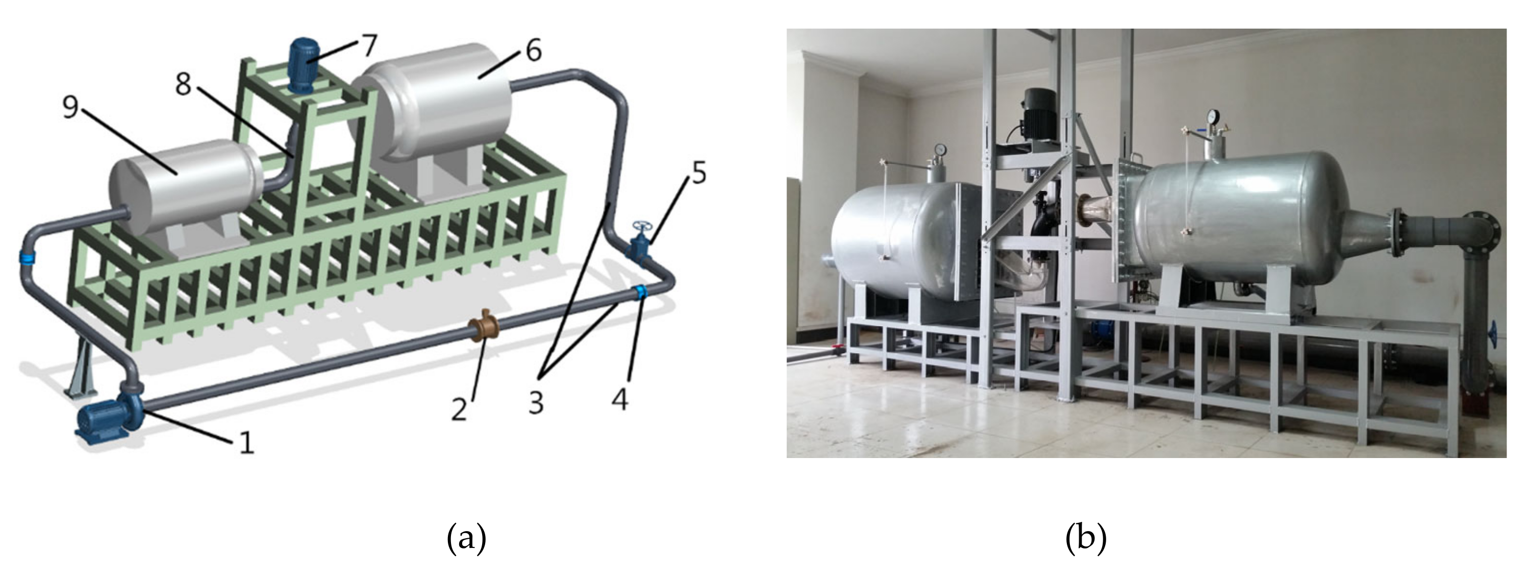
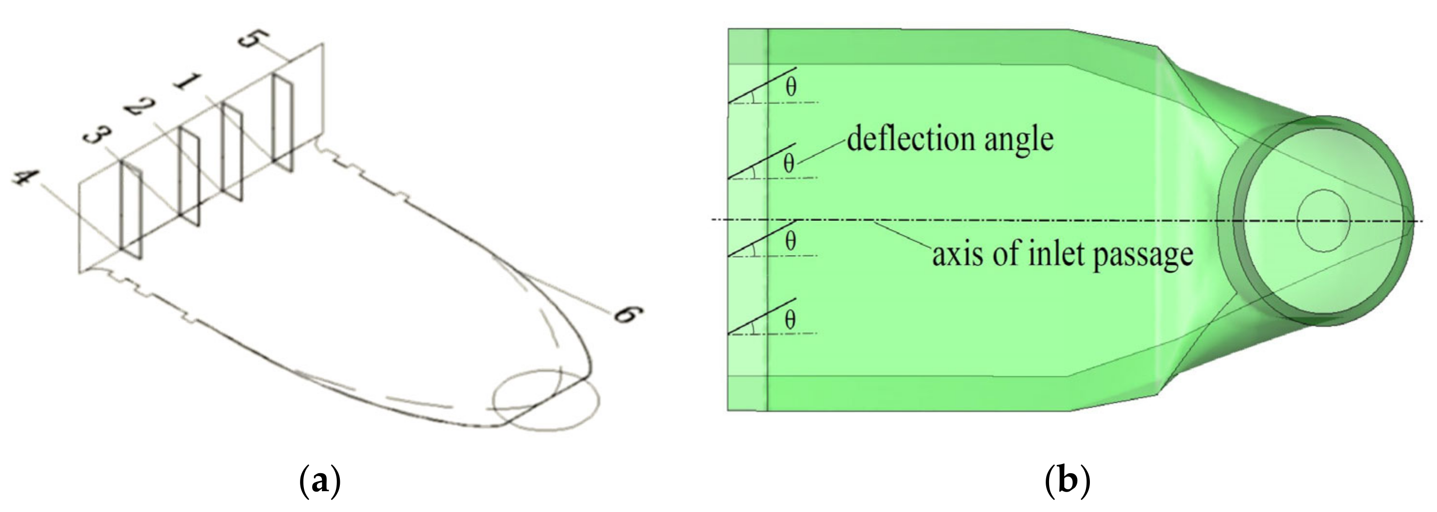
2.1. Pump Device

The vertical axial flow pump device includes five flow parts: inlet passage, impeller, guide vane, elbow and outlet passage. The nominal diameter of the impeller is 120 mm, the hub ratio is 0.40, the number of blades is 4, the blade placement angle is 0°, the average blade tip clearance is 0.2 mm and the impeller speed is 2200 r/min. The number of blades of the guide vane is five. The main dimensions of the elbow inlet passage include: the upper side line inclination angle is 28°, the lower side line inclination angle is 9°, the horizontal projection length of the runner is 3.73 D (D is the nominal diameter of the impeller), and the inlet height of the runner is 1.98 D, the width of the inlet of the runner is 2 D, the outlet section diameter is equal to the nominal diameter of the impeller, and the horizontal projection length of the curved section is 1.23 D. The three-dimensional solid diagram of the pump device is shown in Figure 1.

In this experiment, the deflector plates were used to offset the flow entering the inlet passage, so that the performance difference of the pump device under different deflection angles could be analyzed. The deflector had a thickness of 0.125 D and a length of 0.833 D, which is located at the inlet of the inlet passage. The cross section of the deflector is streamlined and suitable for fluids, and the longitudinal section is rectangular. Four deflector plates with equal intervals were arranged at the inlet of the inlet passage. The schematic diagrams of deflector plates layout and deflection angle are shown in Figure 2. The deflection angle could be changed in the range of −90°~+90°. The deflector was fixed by threads, and connected to the traction device through a lead rod. When the traction device was moved, all the deflectors could be guided in the same direction.

In order to monitor the internal pressure pulsation characteristics of the axial flow pump device, three monitoring points were set at the exit section of the inlet flow passage. If a straight line was drawn to connect each monitoring point with the center point of the exit section, and the angle between every two lines was 120°. The layout of the monitoring points is shown in Figure 3. A 485-20 digital sensor hub and CY302 high precision digital pressure sensor were used to measure pressure pulsation. The probe size of the pressure sensor was 5 mm, the sampling frequency was 1000 Hz, the accuracy was 0.1% FS and the test range was 0~30 kPa.

2.2. Uncertainty Analysis of Experiment

2.2.1. Uncertainty Analysis of Pumping System

Figure 1 shows the sketch of the experimental pump device. There was a long enough straight pipe section in front of the electromagnetic flowmeter to ensure smooth flow into the test instrument and ensure the accuracy of the test. The LDG-125S electromagnetic flowmeter was used for flow measurement, and it was verified before installation. The head of the pumping system was measured by the differential pressure transmitter EJA110A. A JW-3 speed torque sensor was installed between the electric motor and the pump shaft to measure the speed and input torque of the pump shaft.

Efficiency synthesis error is the square sum root of systematic error and random error [21]:

$$E_{\eta }=\pm \sqrt{E_{\eta ,S}^2+E_{\eta ,R}^2}$$

(1)

The total system error of the efficiency of the pump device performance test of the test bench is the root and square of the individual system errors:

$$E_{\eta ,S}=\pm \sqrt{E_{Q·S}^2+E_{H·S}^2+E_{n·S}^2+E_{M·S}^2}$$

(2)

where $E_{Q·S}$ is systematic error of electromagnetic flowmeter, $E_{H·S}$ is systematic error of differential pressure transmitter, $E_{n·S}$ is systematic error of torque speed sensor, and $E_{M·S}$ is systematic error of torque meter. These systematic error parameters are dependent on testing equipment shown in

Table 1. The main equipment of the experimental test system.

Terms	Equipment	Type	Systematic Error
Flow	Electromagnetic flowmeter	EJA110A	±0.1%
Head	Differential pressure	LDG-125S	±0.01%
Torque and speed	Transmitter	JW-3	±0.1%
	Torque speed sensor

.

The total random error can be calculated with the following equation:

$$E_{\eta ,R}=\pm \sqrt{E_{Q·R}^2+E_{H·R}^2+E_{n·R}^2+E_{M·R}^2}$$

(3)

where $E_{Q·R}$ is the random error of efficiency testing, $E_{H·R}$ is the random error of head testing, $E_{n·R}$ is the random error of rotation speed testing, and $E_{M·R}$ is the random error of torque testing.

The systematic error was estimated based on the systematic error of each testing equipment and the previous test experience. The total random error was calculated by the method of probability statistics based on the test data of this pumping system model. The total uncertainty $E_{\eta }$ was ±0.190%.

In order to verify the reliability of the test bench, the vertical axial flow pump device at the speed of 2200 r/min was repeatedly tested under the same test method and operating conditions. The test results are shown in Figure 4. With the increase of the flow rate, the trends of the flow-head curves of the vertical axial flow pump device tested three times are almost the same. The data collected under similar working conditions are very close, indicating the reliability of the test results.

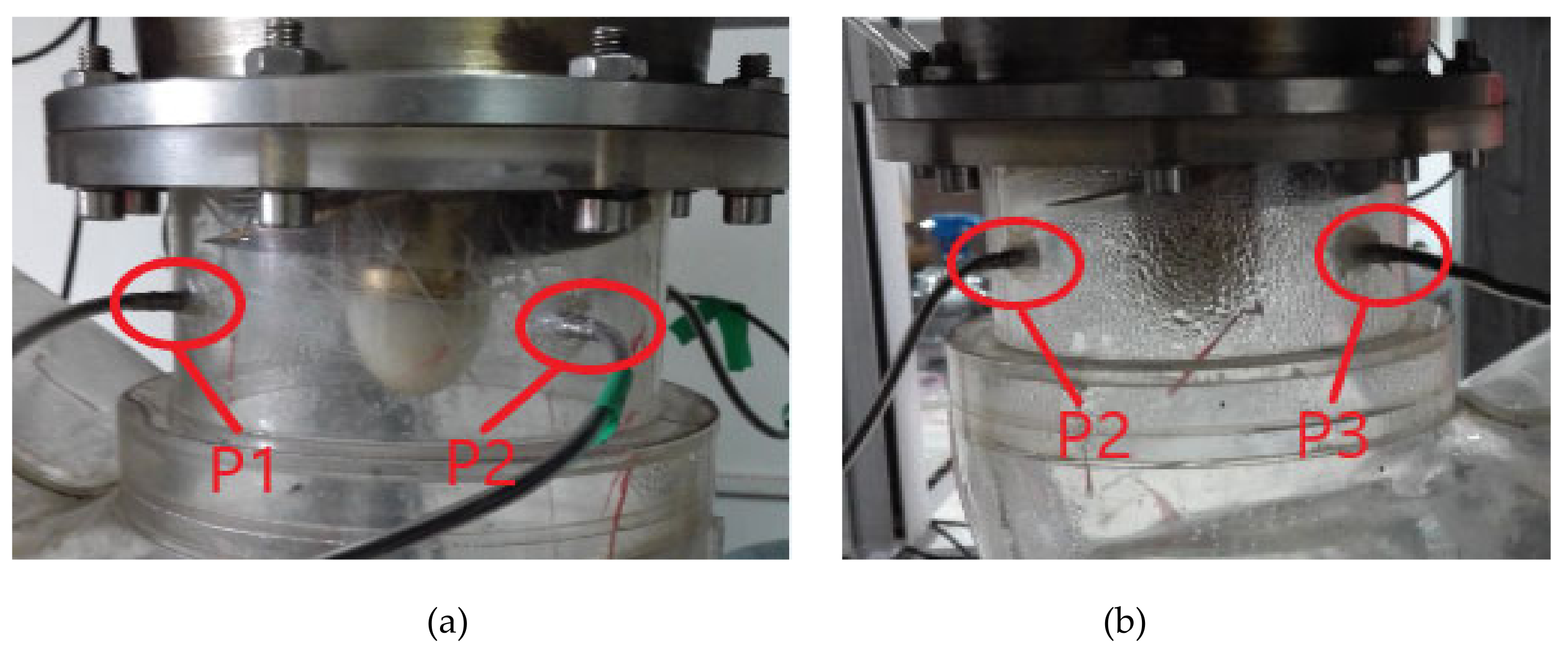
2.2.2. Uncertainty Analysis of Pressure Fluctuation Test

In order to test the reliability of the pressure pulsation test, the monitoring point P1 was tested under the 1.0 Q_bep optimal working condition for the repeatability test at a speed of 2200 r/min and a deflection angle of 0°. The residual error result corresponding to the dominant frequency amplitude is shown in Figure 5. The residual error of the dominant frequency amplitude corresponding to different test results fluctuates around the regression value. The overall deviation amplitude is small, and the collected data results are very close, indicating the pressure pulsation reliability of test results.

3. Numerical Simulation Model and Method

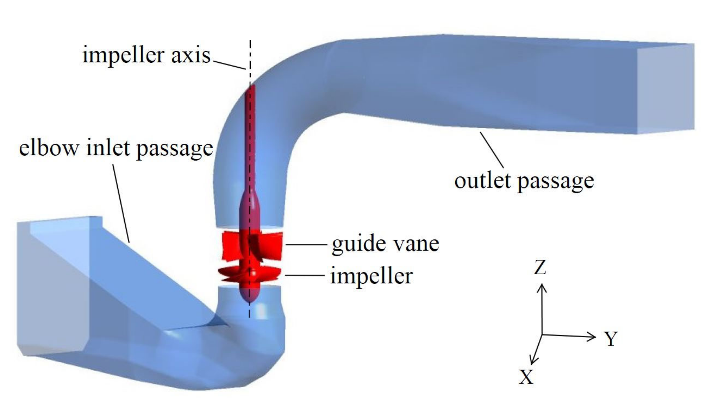
3.1. Numerical Calculation Model

Siemens NX 3D solid modeling software was used to establish 3D solid models of inlet passage, bell pipe, elbow pipe and outlet passage of vertical axial flow pump device. The origin of the reference coordinate system selects the center of the impeller, with Y axis in the water flow direction, X axis perpendicular to the flow direction and Z axis in the impeller axis. The numerical calculation model of the pump device is shown in Figure 6 and Figure 7 shows the inlet passage models with different deflection angles.

In order to facilitate the analysis of the inlet area blockage of deflectors to the elbow inlet at different deflection angles, the inlet area blockage ratio of the deflector was defined as the ratio of the area of the deflector vertically projected on the inlet section to the area of inlet section. The inlet area blockage ratio of the deflector at different deflection angles is shown in

Table 2. Inlet area blockage ratio of deflectors under different deflection angles.

Deflection Angle(°)	Inlet Area Blockage Ratio (%)	Deflection Angle(°)	Inlet Area Blockage Ratio (%)
0	6.07	50	57.31
20	25.21	80	68.54

. Under different flow rate conditions, the inlet area blockage ratio of the deflectors with the same deflection angle at the inlet of the elbow inlet passage was the same.

3.2. Governing Equation and Turbulence Model

The water in the pump device was considered as an incompressible viscous fluid. The governing equation used in the calculation was the Reynolds time-averaged N–S equation. There are many turbulence models suitable for incompressible fluid flow. In the numerical calculation of pump devices, the standard k-ε model is widely used in engineering, and its numerical calculation results and model test results match well [22,23,24,25,26]. The modified turbulent viscosity of the model considers the rotation and rotation flow in the average flow, which can better deal with the flow with high strain rate and large streamline curvature [27]. In this paper, the standard k-ε model was used to numerically calculate the internal flow field of the axial flow pump model under different deflection angles to improve the reliability of the calculation results and predict the performance of the axial flow pump device:

$$\frac{\partial \left(\rho k\right)}{\partial t}+\frac{\partial \left(\rho k{u}_i\right)}{\partial x_i}=\frac{\partial }{\partial x_j}\left[\left(\mu +\frac{u_t}{{\sigma }_k}\right)\frac{\partial k}{\partial x_j}\right]+{\mu }_t\left(\frac{\partial u_i}{\partial x_j}+\frac{\partial u_j}{\partial x_i}\right)\frac{\partial u_i}{\partial x_j}-\rho \epsilon$$

(4)

$$\frac{\partial \left(\rho \epsilon \right)}{\partial t}+\frac{\partial \left(\rho \epsilon u_i\right)}{\partial x_i}=\frac{\partial }{\partial x_j}\left[\left(\mu +\frac{{\mu }_t}{{\sigma }_{\epsilon }}\right)\frac{\partial \epsilon }{\partial x_j}\right]+\frac{C_{1\epsilon }}{k}{\mu }_t\left(\frac{\partial u_i}{\partial x_j}+\frac{\partial u_j}{\partial x_i}\right)\frac{\partial u_i}{\partial x_j}-C_{2\epsilon }\rho \frac{{\epsilon }^2}{K}$$

(5)

where $k$ is the turbulent kinetic energy, $\epsilon$ is the turbulent energy dissipation rate and ${\mu }_t$ is the turbulent viscosity coefficient as shown in Equation (6). ${\sigma }_k$ and ${\sigma }_{\epsilon }$ are the Prandtl numbers corresponding to $k$ and $\epsilon$, respectively.

$${\mu }_t=C_{\mu }\rho \frac{k^2}{\epsilon }$$

(6)

In the standard k-ε model, $C_{1\epsilon }$, $C_{2\epsilon }$, $C_{\mu }$, ${\sigma }_k$ and ${\sigma }_{\epsilon }$ is recommended by experts or empirical value, the values are $C_{1\epsilon }$ = 1.44, $C_{2\epsilon }$ = 1.92, $C_{\mu }$ = 0.09, ${\sigma }_k$ = 1.0 and ${\sigma }_{\epsilon }$ = 1.3.

3.3. Boundary Condition Setting

The commercial 3D CFD code ANSYS-CFX was employed in this work. ANSYS CFX utilizes a finite-element based finite-volume method discrete to the transport equations. The calculation domain of the selected axial flow pump model included five parts: inlet passage, impeller, guide vane, elbow and outlet passage. The inlet of the calculation domain was the inlet of inlet passage, and the inlet boundary condition was set to the total pressure condition, the total pressure at the inlet was set to 1 standard atmospheric pressure, the impeller was a rotating part, and the others were static parts. The dynamic and static interface was set to Stage [28], and the static and static interface was set to None. The impeller speed was 2200 r/min, the outlet of the calculation domain was the outlet of the outlet passage, the outlet boundary condition was set to the mass flow outlet and the wall was smooth without slippage. Scalable wall functions were used in the near wall region. The calculation accuracy was set to 1.0 × 10⁻⁵. The advantage of the scalable wall functions is that no matter how dense the grid is, the logarithmic law formula can always be used to calculate the average velocity without problems. Boundary conditions settings are collected in

Table 3. Boundary conditions setting.

Locations	Type
Inlet of model pump	Total pressure, 1 standard atmosphere
Outlet of model pump	Mass flow rate
Solid wall surface	No-slip wall
Convergence criterion	10−5
Interface on both sides of impeller	Stage
Static and static interface	None

.

3.4. Analysis of Grid Irrelevance of Computational Model

The grids of the pump device in this paper were all structured grids. The H/J/C/L grid method was used to generate the topology of the impeller and the topology was adjusted by adjusting the control points to generate the grid. The ATM Optimized method was used to automatically generate the topology mesh of the guide vane. The minimum surface angle of the mesh generated by the impeller and the guide vane was above 15°, the maximum surface angle was below 165° and the two options of maximum mesh volume rate and maximum boundary mesh rate did not exceed 30%. The grids of the inlet passage, elbow and outlet passage were generated in ICEM software.

Considering that the y+ of the boundary layer grid met the requirements, the analysis of grid number independence is meaningful. y+ represents the distance from the nearest grid node to the wall, which is a dimensionless variable. In the viscous bottom layer, the flow was almost a laminar flow, therefore the viscosity played an absolute role, and the turbulent stress almost did not work. The high Reynolds number turbulence model could not be used to solve the flow in this region. The accuracy of the calculation results could be effectively improved by adjusting the grid y+ value. Referring to the research conclusion of reference [29], the k-ε turbulence model with a high Reynolds number based on wall function was used to solve the internal flow of pump, which requires y+ to meet 30 < y+ < 300. In the optimal working condition, with the increase of the deflection angle, the y+ at inlet passage, impeller, guide vane, elbow and outlet passage were 100~185, 27~28, 46~47, 150~162 and 36~45, respectively, which met the requirements for solving the flow field of the pump device [30]. The grids of inlet passage, impeller, guide vane and outlet passage are shown in Figure 8.

Figure 9 shows the effect of different grid numbers on the energy performance of the pump device at the optimal working condition, comparing the pump head and efficiency under different grid numbers. When the influence error of the increase in the number of grids on the head and efficiency of pump device was within 2%, it was considered that the numerical simulation results were grid-independent. In order to ensure the accuracy of the calculation while saving computing resources, the total number of final grids in the domain was set to 4.51 million.

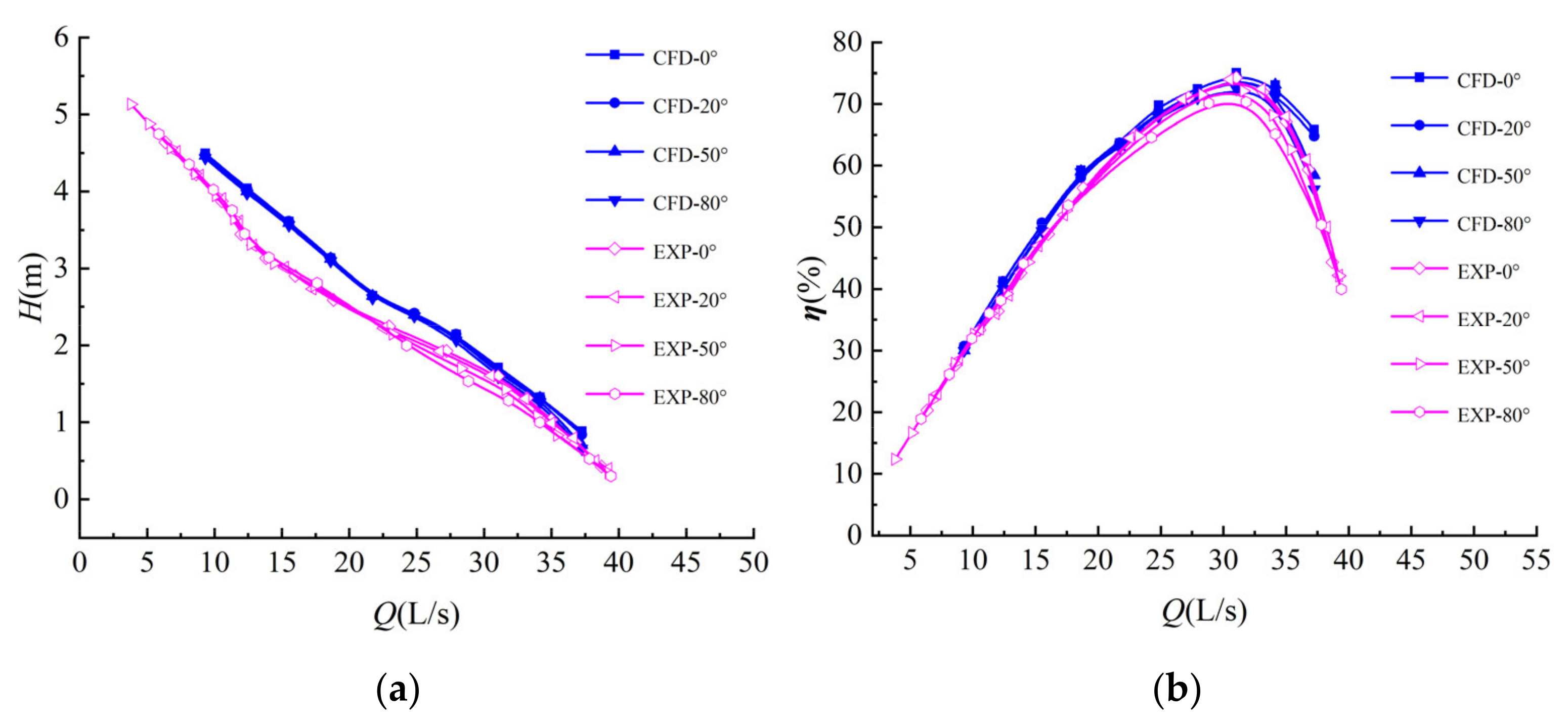
3.5. Validation of the Numerical Simulation

In order to further verify the validity of the numerical calculation results, the physical model test of the pump device was carried out on the hydraulic machinery test bench of the Jiangsu Key Laboratory of Water Conservancy and Power Engineering. The test bench is composed of a water outlet tank, PVC pipe, ISWH125-100A type 304 stainless steel pipe centrifugal pump and steel soft sealing butterfly valve, which is shown in Figure 1. The inlet and outlet sections of the electromagnetic flowmeter have straight pipe sections with a length greater than 5D, which ensures the stable and smooth water flow into the electromagnetic flowmeter and ensures the accuracy of measurement. The comparison between the numerical prediction results of the energy performance of the pump device and the physical model test results is shown in Figure 10.

With the change of the deflection angle, the flow-head curve and flow-efficiency curve corresponding to numerical simulation and model test results of pump device have no obvious changes at low-rate flow conditions, which is related to the unstable turbulent flow under low-rate flow conditions. The digital simulation results of the flow-head curve and the flow-efficiency curve are basically higher than the test results. At the deflection angles of 0°, 20°, 50° and 80°, the maximum efficiency points of the numerical simulation are 0.767%, 0.456%, 1.649% and 2.093% higher than the test results, respectively. This is due to the differences in boundary conditions between numerical simulation and experiment, e.g., the wall of the flow passage was set to a smooth wall in the numerical simulation, and the wall of the experiment was obviously not smooth. In general, the performance curves predicted by the numerical simulation were generally in good agreement with the test results. Qualitative agreement of the dependence of global characteristics on the flow intensity proves that the theoretical model was qualitatively correct. So, it can be used for the detailed but rather qualitative analysis of the structure of the flow in the pump.

4. Results and Analysis

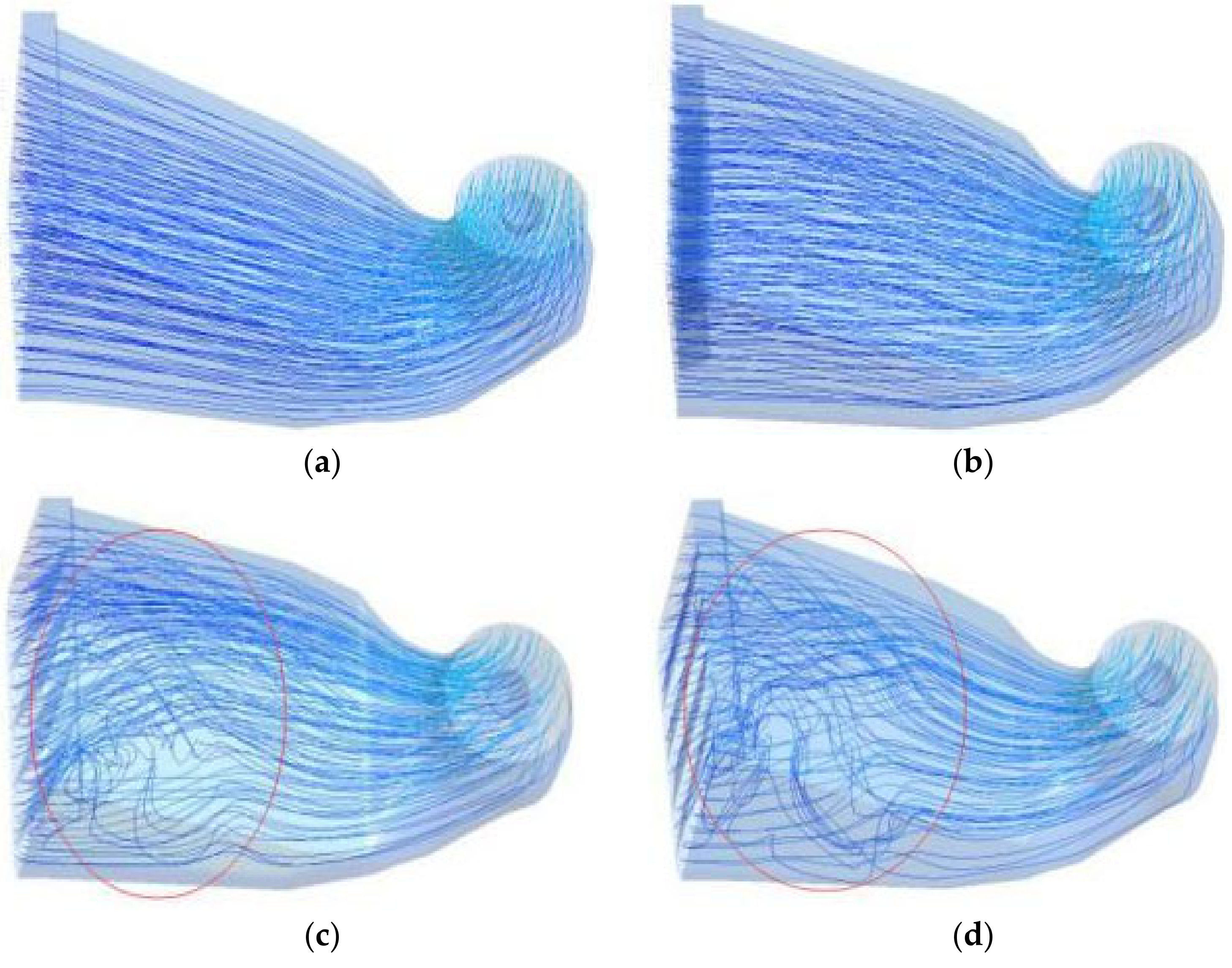
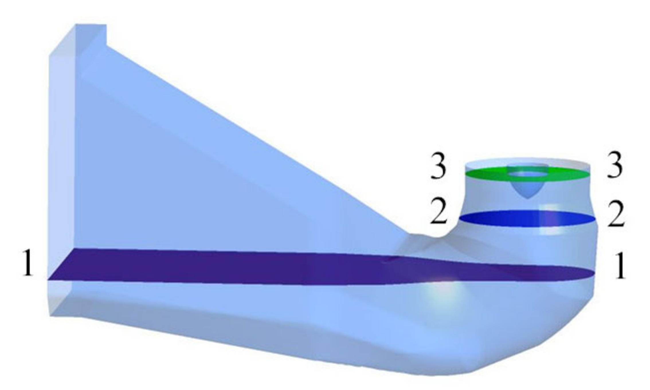
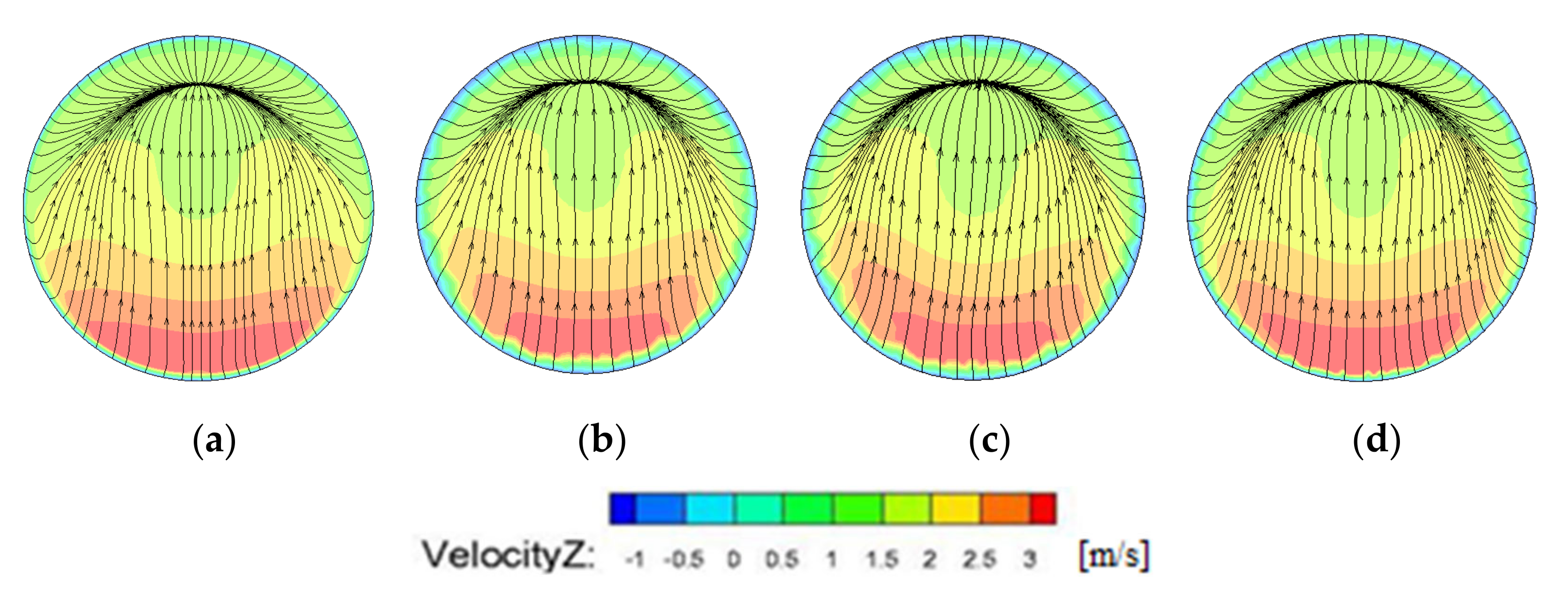
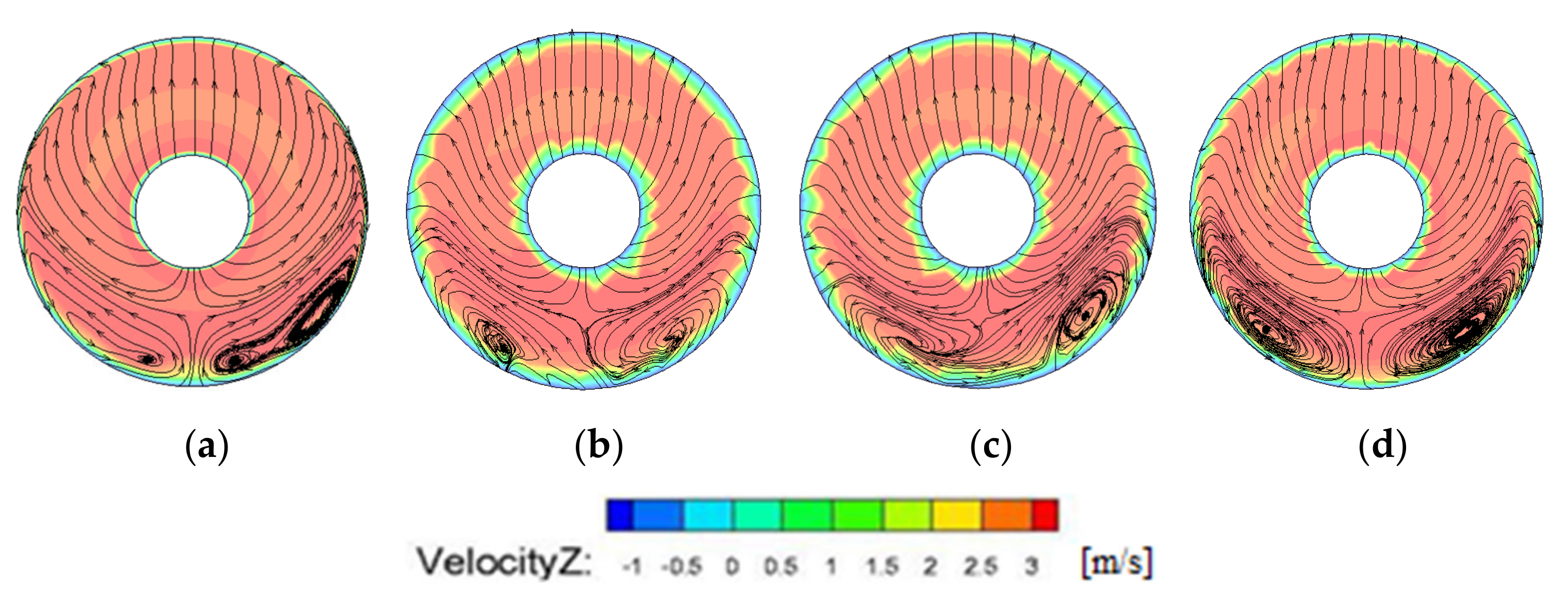
4.1. Analysis of Flow Characteristics in Inlet Passage

In order to study the variation law of the internal flow in the axial flow pump under different deflection angles, the three-dimensional flow field inside the inlet passage with different deflection angles was analyzed under the optimal working conditions. At the deflection angle of 0°, the water in the inlet passage flowed smoothly from the inlet to the horn. At the deflection angle of 20°, the water flow at the inlet of the inlet passage was slightly offset upwards, and the overall streamline had no significant change compared with deflection angle of 0°, so the flow was relatively smooth. At the deflection angle of 50°, due to the guiding effect of the deflector, the flow at the front of the inlet passage significantly deviated, the streamline was inclined upward and a local vortex band was formed below the inlet passage, the flow streamline near the horn tube was relatively smooth. At the deflection angle of 80°, the flow pattern of the flow was more turbulent than the deflection angle of 50° and the disturbance was obvious. The streamline offset range was expanded, and the streamline near the horn tube had a small range of offset, which was related to the forward movement of vortex band driven by flow. The three-dimensional streamline diagram is shown in Figure 11.

In order to further analyze the flow characteristics of the flow in the inlet passage, three sections were selected to analyze the changes of the flow pattern in inlet passage at the optimal working condition and different deflection angles. The schematic diagram of the position of the sections is shown in Figure 12, in which section 1-1 is located in the middle section of the inlet passage, and sections 2-2 and 3-3 are located inside the horn tube.

Figure 13 shows the streamline and axial velocity distribution (Y direction) of section 1-1.

At the deflection angle of 0°, the flow velocity first increases and then decreases along the axis direction of the inlet passage. The velocity near the elbow is the maximum, and the axial velocity under the horn is the minimum. There are three high velocity zones at the elbow, which are symmetrically distributed. At the deflection angle of 20°, the low velocity zones caused by the deflector plates from the leftmost to the rightmost are distributed in parallel, and the area of the low velocity areas is increasing compared with the deflection angle of 0°. There are small-scale vortices near each deflector. Due to the impact of water flow, there is a local high velocity area near the right wall. Compared with deflection angle of 0°, the high velocity area at the elbow shifts to the left, and the high velocity area at the right side of the elbow gradually disappears, which is related to the deviation of the streamline to the left. At the deflection angle of 50°, the area of the low velocity zone caused by the rightmost deflector expands, forming two large-scale vortex bands in the low velocity area, and there is a small range of high velocity area on the right wall. Due to the overall flow shift to the left side, the elbow high velocity area is expanded and irregular. At the deflection angle of 80°, due to the strong guiding effect of the deflector, there are local high velocity areas generated at intervals near the left and right walls. The low velocity area caused by the deflector on the rightmost is larger than that caused by the 50° deflector, and the low velocity area near each deflector is irregularly distributed. The high velocity area at the elbow is similar to that caused by the 20° deflector, but the area of the high velocity zone increases.

Figure 14 and Figure 15 show the contours of streamline and axial velocity distribution (Z direction) in 2-2 and 3-3.

Due to the contraction of water flow and the rotation of impeller, the flow velocity from section 2-2 to section 3-3 generally shows an overall increasing trend. With the increase of the deflection angle, the 2-2 section shows the increase trend with the increase of the deflection angle, but the velocity field shifts slightly to the right. According to the streamline diagram, due to the backflow of the side wall, the streamline is mainly concentrated above the section. At the deflection angles of 20°, 50° and 80°, the flow velocity at the side wall of section 2-2 is different from the 0° deflection angle, and the area of the high velocity area below slightly decreases with the change of the deflection angle. Since the 3-3 section is close to the inlet side of the impeller, there are two vortex bands on both sides at different deflection angles. Except for the 0° deflection angle, there is a small area of low velocity near the side wall and the middle ring of the other deflection angles. At the deflection angle of 50°, the right vortex shifts to the left, and the range of vortex band slightly increases at the 80° deflection angle.

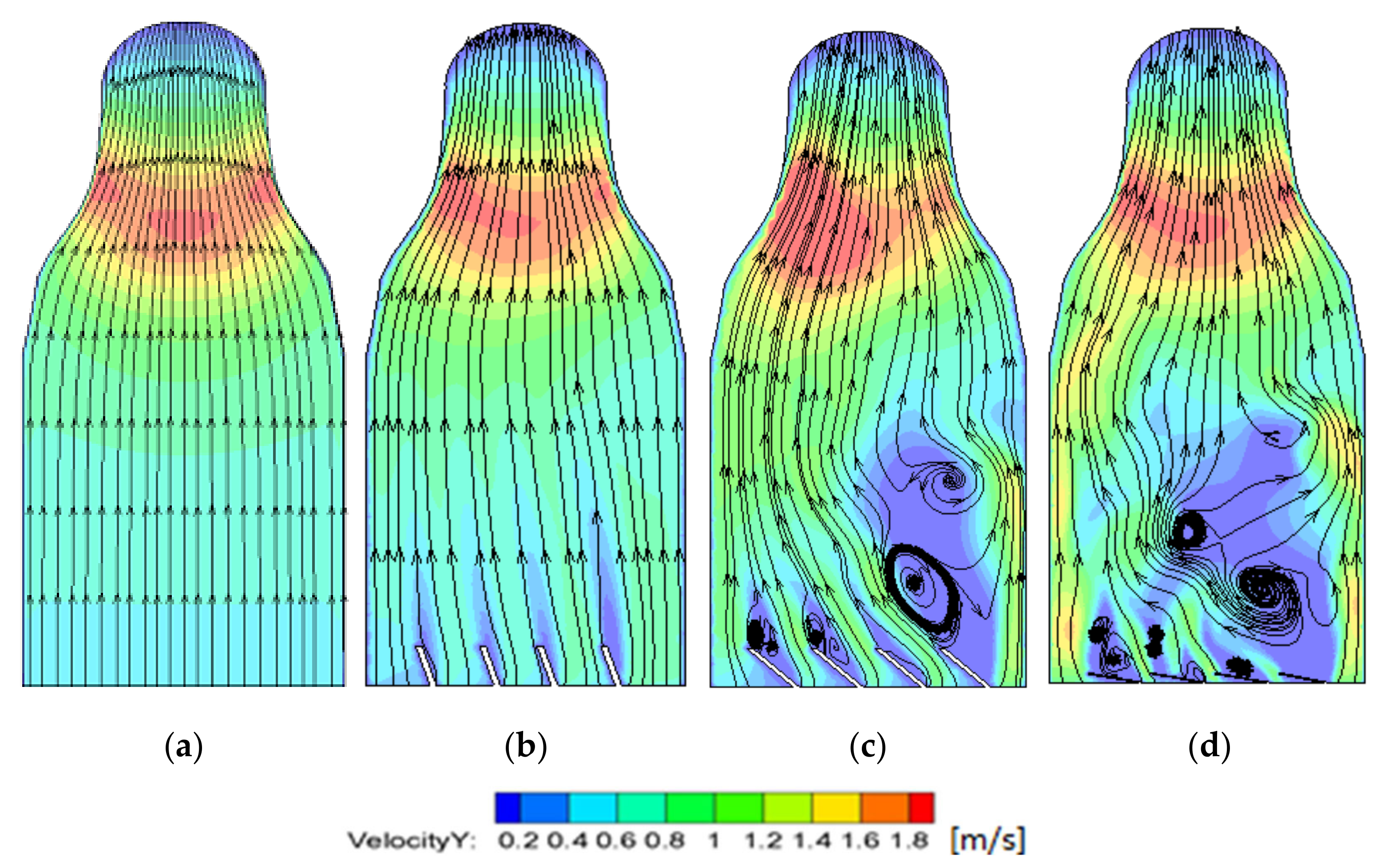
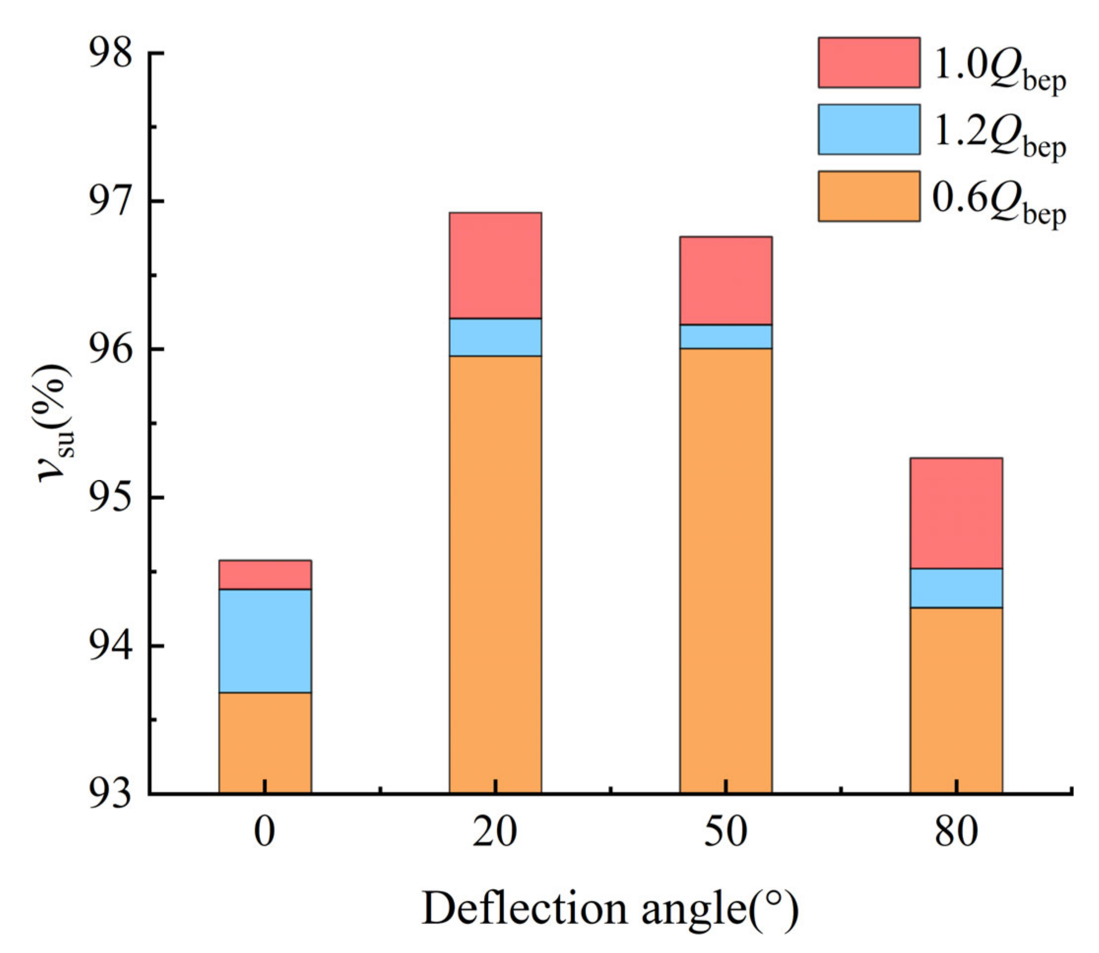
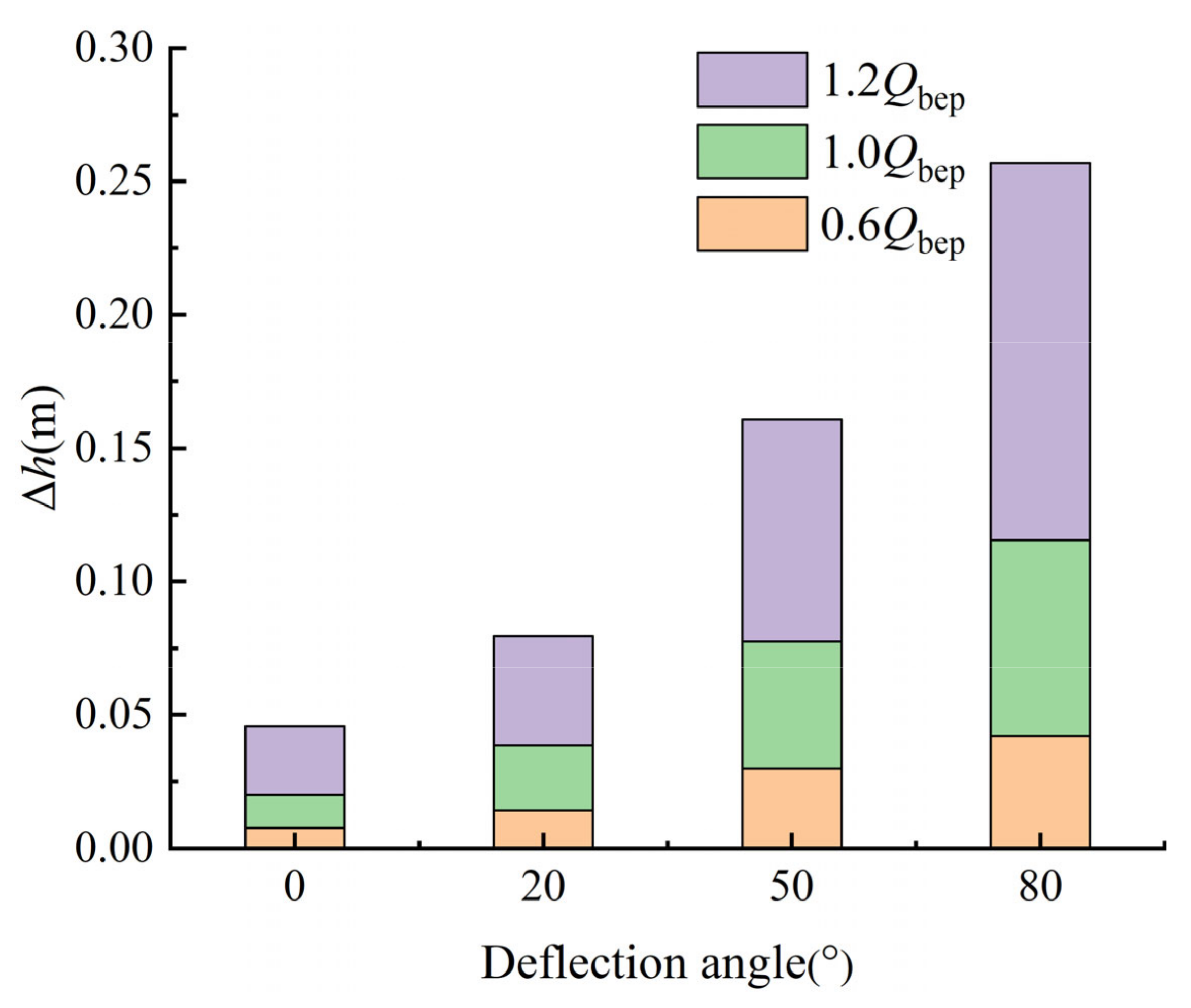
4.2. Analysis of Axial Velocity Uniformity at Outlet of Inlet Passage and the Hydraulic Loss of Inlet Passage

The axial velocity distribution uniformity v_su of the outlet section of the inlet passage and the hydraulic loss of the inlet passage are introduced to analyze the hydraulic performance of the elbow inlet passage under different deflection angles. The uniformity of the outlet flow velocity can be used to quantitatively reflect the distribution of the outlet flow velocity of the inlet passage, which is an important indicator for evaluating the hydraulic characteristics of the inlet passage. The uniformity of flow velocity distribution is represented by v_su, v_su = 100% is the ideal situation, and the calculation formula is as follows:

$$v_{\mathrm{su}}=[1-\frac{1}{\overline{v_a}}\sqrt{\frac{{{\displaystyle \sum }}_{i=1}^n{\left(v_{\mathit{ai}}-\overline{v_a}\right)}^2\Delta A_i}{{{\displaystyle \sum }}_{i=1}^n\Delta A_i}}]\times 100\%$$

(7)

$$\overline{v_a}=\frac{Q}{A}$$

(8)

where $\overline{v_a}$ is the average axial velocity of the impeller inlet section, $v_{\mathit{ai}}$ is the axial velocity of the i-th grid of the impeller inlet section, $\Delta A_i$ is the area of the i-th cell, $n$ is the total number of grids of the section.

The change of flow velocity uniformity at the outlet of the inlet passage under different working conditions and deflection angles is shown in Figure 16.

With the increase of the deflection angle, the flow velocity uniformity first increases and then decreases. At the optimal working condition, when the deflection angle is 0°, the minimum uniformity of the axial velocity distribution at the outlet of the inlet passage is 94.58%, which can meet the requirements of the runner for inlet conditions. Combined with the three-dimensional flow field diagram of the inlet passage, the influence of the deflection angle on the uniformity of the outlet flow velocity of the inlet passage is not positively correlated, which is related to the influence range of the deflector plates on the flow pattern of the inlet passage.

Hydraulic loss of the inlet passage is an important indicator of the energy consumption evaluation of pumping station. The hydraulic loss is represented by $\Delta h$ and the calculation formula is as follows:

$$\Delta h=\frac{P_{\mathit{in}}{-P}_{\mathit{out}}}{\rho g}=\frac{{\left[\frac{1}{A}{{\displaystyle \sum }}_{i=1}^n{p}_i\left|A_i\right|\right]}_{in}-{\left[\frac{1}{A}{{\displaystyle \sum }}_{i=1}^n{p}_i\left|A_i\right|\right]}_{out}}{\rho g}$$

(9)

where $P_{\mathit{in}}$ is the pressure at the inlet section of the inlet passage, $P_{\mathit{out}}$ is the pressure at the outlet section of the inlet passage, $\rho$ is the density of water, $g$ is the local gravity acceleration, $A_i$ is the area of the i-th grid, p_i is the pressure of the i-th grid and $\Delta h$ is the hydraulic loss.

The variation curve of hydraulic loss of inlet passage with deflection angle at different working conditions is shown in Figure 17.

At different working conditions, with the increase of the deflection angle, the hydraulic loss of the inlet passage increases continuously, which is related to the change of the flow pattern in the inlet passage under different deflection angles. The flow is impacted by the guiding action of the deflector on the sidewall of the inlet pool, and hydraulic loss increases continuously due to friction. In high-rate flow conditions, the increase of liquid particle velocity and kinetic energy is also the cause of hydraulic loss greater than the other two conditions. The change of the flow pattern in the inlet passage under different deflection angles leads to the difference of hydraulic loss in the inlet passage. At the optimal working condition, when the deflection angle is 0°, the hydraulic loss of the inlet passage is 0.0202 m, and when the deflection angle is 80°, the hydraulic loss of the inlet passage is 0.1155 m, which is about six times that of the 0° deflection angle.

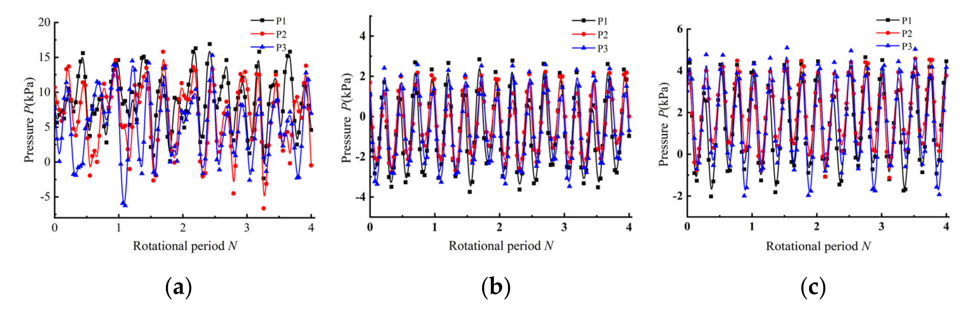
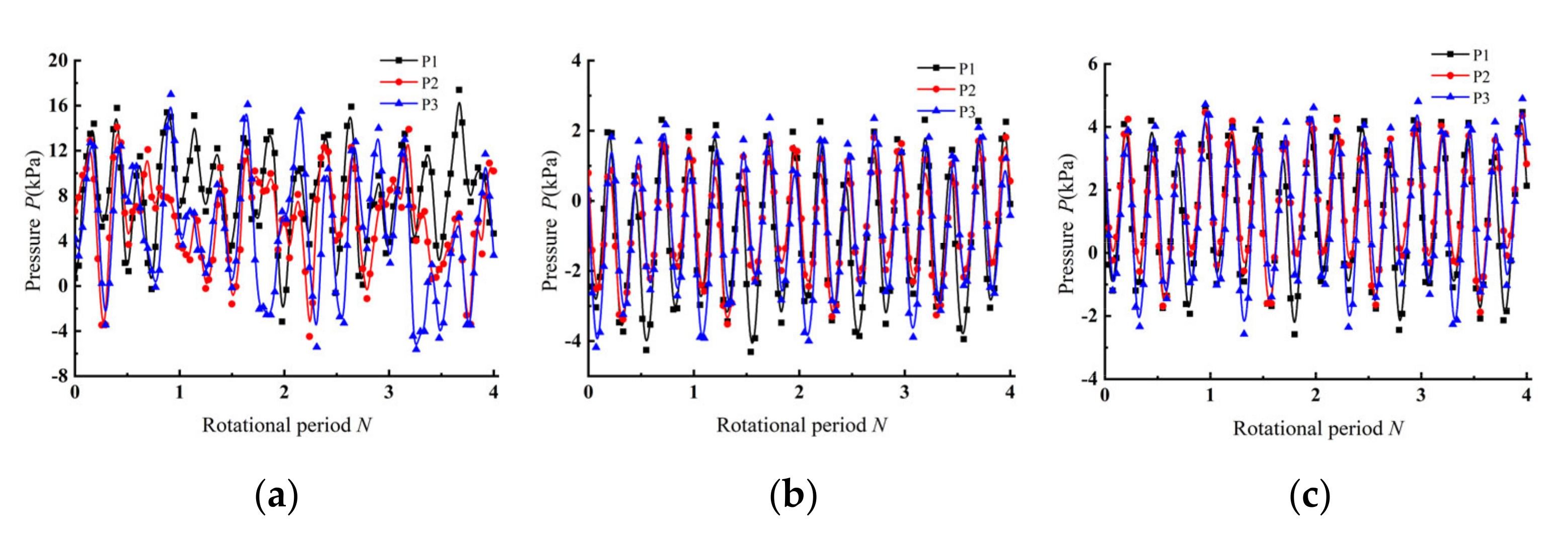
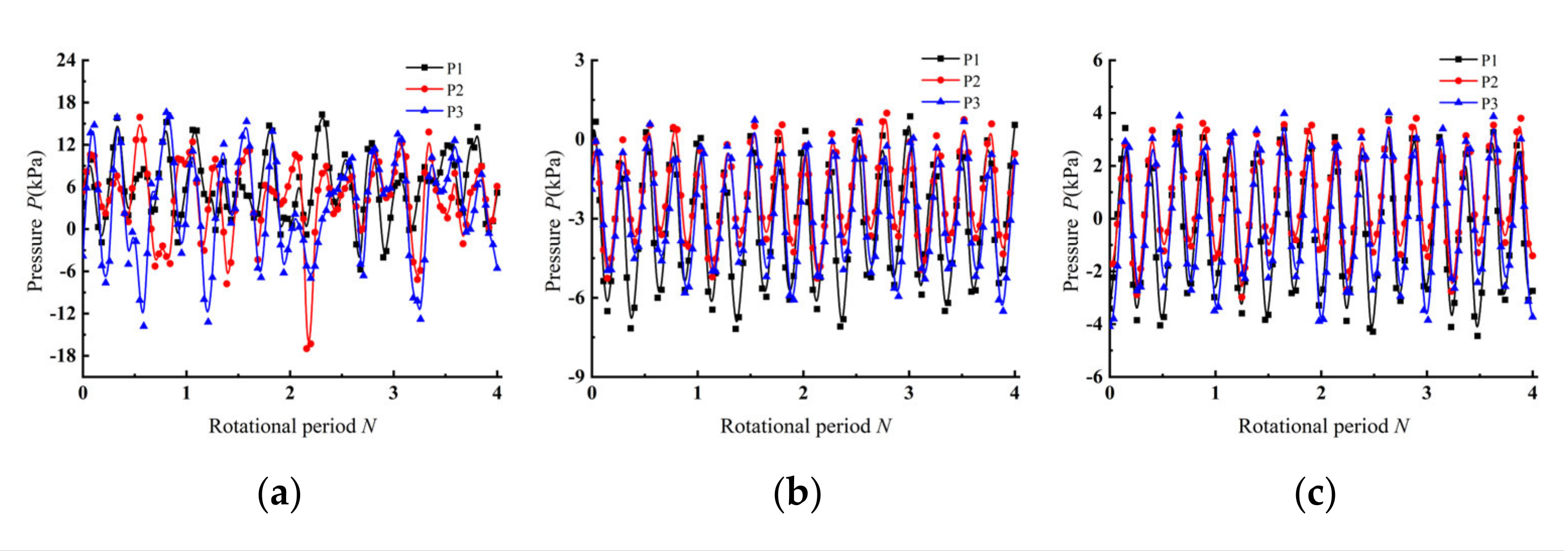
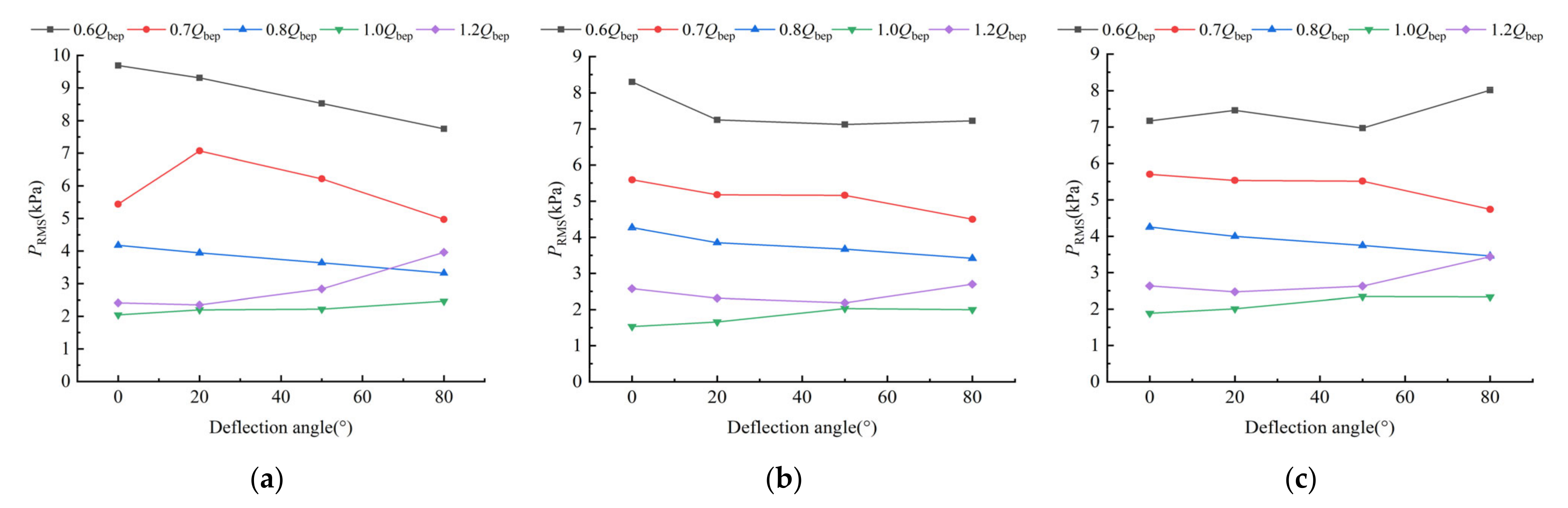
4.3. Time Domain Analysis of Pressure Pulsation at the Outlet Monitoring Point of the Inlet Passage

As is shown in Figure 18, Figure 19, Figure 20 and Figure 21, the time-domain data of the pressure pulsation in the inlet passage has obvious regularity. The pressure and time of the monitoring points are sinusoidal, and the pressure fluctuation is obvious, indicating that the disturbance of the blade on the flow has occurred before the flow enters the impeller. There are four wave crests and four wave troughs in one cycle of the impeller rotation, and the number of crests and troughs is equivalent to the number of impeller blades. Due to the influence of the limited number of blades, there is a large pressure gradient from the pressure surface to the suction surface of the impeller blades. During the rotation of the impeller, the pressure pulsation in front of the impeller alternates. In low-rate flow condition of 0.6 Q_bep, due to the strong irregular motion of turbulence in the pump and the tip vortex, the pressure fluctuation at the outlet monitoring point of the inlet appears the second peak phenomenon in some cycles, and there are multiple peaks in a sine wave shape. As the flow rate increases, the pulsation amplitude of each monitoring point decreases first and then increases, and the pressure pulsation amplitude is the minimum under optimal conditions. Compared with 0.6 Q_bep low flow condition, the secondary wave peaks in some periods disappear and the waveform is more periodic in 1.0 Q_bep and 1.2 Q_bep flow conditions. In a high-rate flow condition of 1.2 Q_bep, there is a local backflow phenomenon in the impeller inlet section and the pulsation amplitude shows an increasing trend.

Under the same working condition, with the increase of the deflection angle, the overall waveform of the time domain shifts to the negative pressure. The peak value of each monitoring point first decreases and then increases with the increase of the flow rate. Under the optimal working condition, the peak value is the minimum, and the time-domain waveform of each monitoring point has little different between the optimum working condition and the high-rate flow condition.

Figure 22 shows the root-mean-square pressure pulsation values of each monitoring point under different deflection angles. RMS is the root mean square value, which has a small degree of numerical dispersion and can better characterize the energy level of pressure pulsation. It is one of the main parameters of signal amplitude analysis. The root mean square P_RMS of the pulsation amplitude is calculated as follows:

$$P_{RMS}=\sqrt{\frac{P_1^2+P_2^2+\dots +P_n^2}{n}}$$

(10)

where $P_n$ is the n-th measurement of pressure, n is the number of collected data.

With the increase of flow rate, the RMS value of pressure pulsation at different monitoring points decreases first and then increases. The RMS value of pressure pulsation is maximum at 0.6 Q_bep low-rate flow condition and minimum at 1.0 Q_bep optimal flow rate condition. Under 0.6 Q_bep low-rate flow condition, the RMS values of pressure pulsation of monitoring points 1 and 2 decrease with the increase of the deflection angle, while the RMS values of pressure pulsation of monitoring point 3 increase with the increase of the deflection angle overall. There may exists a reflux area in the outlet section of the inlet passage under the low-rate flow condition, and the influence range of the reflux area is different, resulting in differences in the flow velocity and pressure fluctuation of flow in the same section. Under the flow conditions of 0.7 Q_bep and 0.8 Q_bep, the RMS value of pressure pulsation of the three monitoring points decreases with the increase of the deflection angle overall. Under the flow conditions of 1.0 Q_bep and 1.2 Q_bep, the RMS value of pressure pulsation of three monitoring points increases with the increase of the deflection angle. The variation trend of RMS value of pressure fluctuation at inlet passage outlet with the increase of deflection angle under different flow conditions is different, which may be related to the difference of internal flow pattern of inlet passage under different flow conditions.

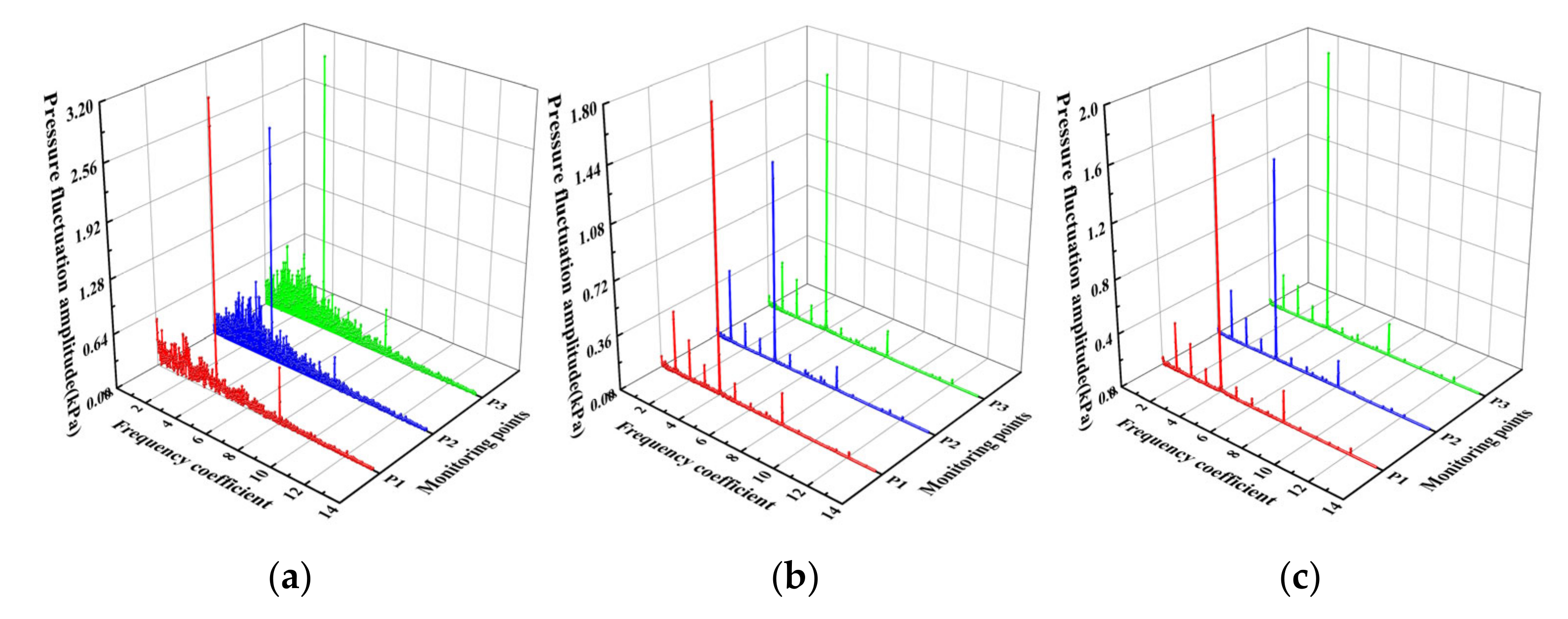
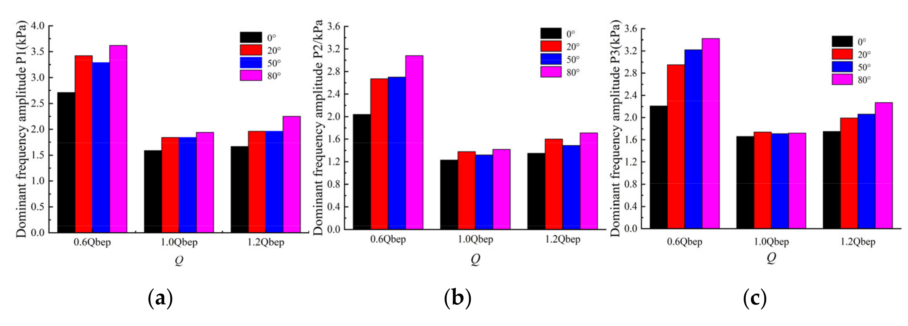
4.4. Frequency Domain Analysis of Pressure Pulsation at the Outlet Monitoring Point of the Inlet Passage

Figure 23, Figure 24, Figure 25 and Figure 26 shows the pulsation spectrum of the three monitoring points at the outlet section of the elbow inlet passage at different deflection angles. The frequency is expressed by the multiple frequency $N_F$, the calculation formula is as follows:

$$N_F=\frac{60F}{n}$$

(11)

where $F$ is the corresponding frequency value after short-time Fourier transform; $n$ is the rotating speed.

As shown in Figure 23, Figure 24, Figure 25 and Figure 26, the dominant pulsation frequencies of the three monitoring points at different deflection angles are all four times of the rotational frequency, and the frequency range corresponding to the larger amplitude is 0~8 times of the rotational frequency. Due to the difference in the layout of monitoring points, the influence of water flow on the dominant frequency amplitude of each monitoring point shows a certain regularity. Under different working conditions, the dominant frequency amplitude of the monitoring point from P1 to P3 first decreases and then increases, and the dominant frequency amplitude of the monitoring point P2 is the minimum. Under 0.6 Q_bep low-rate flow condition, due to the strong irregular movement of the turbulence in the pump, there are more low-frequency pulsation components below four times the rotational frequency under different deflection angles, which has a certain relationship with the irregular movement of turbulent flow in the pump under low-rate flow conditions. Under different deflection angles and different working conditions, the amplitude of frequency doubling and harmonic frequency corresponding to each monitoring point decreases from one to three times, and the amplitude increases to the maximum at four times, and the amplitude increases at eight times.

Figure 27 shows the dominant frequency amplitude diagram of each monitoring point at the outlet of the inlet passage with different deflection angles. The dominant frequency amplitude of three monitoring points at the outlet of inlet passage shows an overall increasing trend with the increase of the deflection angle under 0.6 Q_bep low-rate flow condition. The difference between the maximum dominant frequency amplitude and the minimum dominant frequency amplitude of monitoring points 1, 2 and 3 is 0.91 kPa, 1.04 kPa and 1.21 kPa, respectively. Under the optimal condition of 1.0 Q_bep, the dominant frequency amplitude of the three monitoring points changes little with the increase of the deflection angle, indicating that the variation of the deflection angle has little effect on the pulsation characteristic at the outlet of inlet passage under the optimal condition of 1.0 Q_bep. The difference between the maximum and minimum dominant frequency amplitudes of monitoring points 1, 2 and 3 is just 0.4 kPa, 0.19 kPa and 0.08 kPa, respectively. Under high-rate flow conditions, the dominant frequency amplitude of each monitoring point basically increases with the increase of deflection angle. The difference between the maximum dominant frequency amplitude and the minimum dominant frequency amplitude of monitoring points 1, 2 and 3 is 0.58 kPa, 0.36 kPa and 0.52 kPa, respectively. The variation of the dominant frequency amplitude of each monitoring point with the variation of the deflection angle is dominated by the 0.6 Q_bep low-rate flow condition, and the dominant frequency amplitude changes little under other flow conditions. The variation of deflection angle has the greatest effect on the dominant frequency amplitude of monitoring points under 0.6 Q_bep low-rate flow condition and the little effect under 1.0 Q_bep optimal flow condition.

In this paper, the authors studied the variation of the flow characteristics in the inlet passage of an axial flow pump device with variation of the deflection angle by arranging the deflector plates at the inlet of the inlet passage. The results of a numerical simulation and a model test were compared and verify the accuracy and reliability of numerical simulation. The numerical simulation method was used to analyze the flow velocity and flow pattern changes of different sections of inlet passage. By means of physical model test, the variation of time domain and frequency domain of pressure fluctuation at monitoring points at outlet of inlet passage with the change of flow rate and deflection angle was analyzed.

Due to the guiding effect of the deflector plates, the streamline in the inlet passage became chaotic with the increase of the deflection angle, and the scale and scope of the vortex in the inlet passage expanded with the increase of the deflection angle. Under the optimal flow condition of 1.0 Q_bep, the increase of the deflection angle had a negative impact on the flow pattern in the inlet passage. The maximum velocity was generated near the elbow and the minimum axial velocity was generated below the horn at different deflection angles. There was an obvious vortex band in the horn tube which was parallel to the axis of the inlet passage, and the vortex band expanded with the increase of the deflection angle.

The hydraulic loss of inlet passage increased with the increase of the deflection angle. Under the optimal flow condition of 1.0 Q_bep, the hydraulic loss of inlet passage at the deflection angle of 0° was six times that at the deflection angle of 80°. The flow velocity uniformity at the outlet of inlet passage first increased and then decreased with the increase of the deflection angle, while the variation with a small range.

The time-domain waveform of pressure fluctuation at outlet of inlet passage has obvious periodicity under different deflection angle. There were four peaks and four valleys in the pressure fluctuation during a period of impeller rotation, and the number of peaks and valleys is equal to the number of impeller blades. The effect of deflection angle on the dominant frequency amplitude at outlet of the inlet passage monitoring points was smaller under the optimal flow condition of 1.0 Q_bep than under 1.2 Q_bep flow condition and 0.6 Q_bep flow condition, which indicates that the variation of the deflection angle has a greater impact on the hydraulic performance of the inlet passage when the pump device deviates from the optimal flow condition.

References

1. Liu, C. The developments of axial flow pump system researches in China. In Proceedings of the Fluids Engineering Division Summer Meeting, Washington, DC, USA, 10–14 July 2016. [Google Scholar]
2. Yang, F.; Liu, C.; Tang, F.; Zhou, J.; Luo, C. Analysis of hydraulic performance for vertical axial-flow pumping system with cube-type inlet passage. Trans. Chin. Soc. Agric. Eng. 2014, 30, 62–69. [Google Scholar]
3. Jiao, W.; Cheng, L.; Zhang, D.; Zhang, B.; Su, Y.; Wang, C. Optimal design of inlet passage for waterjet propulsion system based on flow and geometric parameters. Adv. Mater. Sci. Eng. 2019, 2019, 2320981. [Google Scholar] [CrossRef] [Green Version]
4. Zhang, D.S.; Shi, W.D.; Bin, C.; Guan, X.F. Unsteady flow analysis and experimental investigation of axial-flow pump. J. Hydrodyn. 2010, 22, 35–43. [Google Scholar] [CrossRef]
5. Zhang, W.P.; Shi, L.J.; Tang, F.P.; Duan, X.H.; Liu, H.Y.; Sun, Z.Z. Analysis of inlet flow passage conditions and their influence on the performance of an axial-flow pump. Proc. Inst. Mech. Eng. Part A-J. Power Energy 2020, 235, 733–746. [Google Scholar] [CrossRef]
6. Liu, C.; Jin, Y. Numerical Simulation on three dimensional flow in two-way reversible pumping system. Trans. Chin. Soc. Agric. Eng. 2011, 42, 74–78. [Google Scholar]
7. Tokyay, T.E.; Constantinescu, S.G. Validation of a large-eddy simulation model to simulate flow in pump intakes of realistic geometry. J. Hydraul. Eng.-ASCE. 2006, 132, 1303–1315. [Google Scholar] [CrossRef]
8. Yang, F.; Xie, C.L.; Liu, C.; Yuan, Y.; Shi, L.J. Influence of axial-flow pumping system operating conditions on hydraulic performance of elbow inlet conduit. Trans. Chin. Soc. Agric. Eng. 2016, 47, 15–21. [Google Scholar]
9. Zhang, D.S.; Shi, W.D.; Pan, D.Z.; Dubuisson, M. Numerical and experimental investigation of tip leakage vortex cavitation patterns and mechanisms in an axial flow pump. J. Fluids Eng.-Trans. ASME 2015, 137, 121103. [Google Scholar] [CrossRef]
10. Xie, C.L.; Tang, F.P.; Zhang, R.T.; Zhou, W.; Zhang, W.P.; Yang, F. Numerical calculation of axial-flow pump’s pressure fluctuation and model test analysis. Adv. Mech. Eng. 2018, 10, 1687814018769775. [Google Scholar] [CrossRef]
11. Choi, Y.D.; Kurokawa, J.; Matsui, J. Performance and internal flow characteristics of a very low specific speed centrifugal pump. J. Fluids Eng.-Trans. ASME 2006, 128, 341–349. [Google Scholar] [CrossRef]
12. Kan, K.; Zheng, Y.; Chen, Y.J.; Xie, Z.S.; Yang, G.; Yang, C.X. Numerical study on the internal flow characteristics of an axial-flow pump under stall conditions. J. Mech. Sci. Technol. 2018, 32, 4683–4695. [Google Scholar] [CrossRef]
13. Mu, T.; Zhang, R.; Xu, H.; Zheng, Y.; Fei, Z.D.; Li, J.H. Study on improvement of hydraulic performance and internal flow pattern of the axial flow pump by groove flow control technology. Renew. Energy 2020, 160, 756–769. [Google Scholar] [CrossRef]
14. Wang, L.; Liu, H.L.; Wang, K.; Zhou, L.; Jiang, X.P.; Li, Y. Numerical Simulation of the Sound Field of a Five-Stage Centrifugal Pump with Different Turbulence Models. Water 2019, 11, 1777. [Google Scholar] [CrossRef] [Green Version]
15. Chen, E.Y.; Ma, Z.L.; Zhao, G.P.; Li, G.P.; Yang, A.L.; Nan, G.F. Numerical investigation on vibration and noise induced by unsteady flow in an axial-flow pump. J. Mech. Sci. Technol. 2016, 30, 5397–5404. [Google Scholar] [CrossRef]
16. Furukawa, A.; Shigemitsu, T.; Watanabe, S. Performance test and flow measurement of contra-rotating axial flow pump. J. Therm. Sci. 2007, 16, 7–13. [Google Scholar] [CrossRef]
17. Feng, J.J.; Luo, X.Q.; Guo, P.C.; Wu, G.K. Influence of tip clearance on pressure fluctuations in an axial flow pump. J. Mech. Sci. Technol. 2016, 30, 1603–1610. [Google Scholar] [CrossRef]
18. Zhang, W.P.; Tang, F.P.; Shi, L.J.; Hu, Q.J.; Zhou, Y. Effects of an inlet vortex on the performance of an axial-flow pump. Energies 2020, 13, 2854. [Google Scholar] [CrossRef]
19. Momosaki, S.; Usami, S.; Watanabe, S.; Furukawa, A. Numerical simulation of internal flow in a contra-rotating axial flow pump. In IOP Conference Series: Earth and Environmental Science, Volume 12, 25th IAHR Symposium on Hydraulic Machinery and Systems 20–24 September 2010 ‘Politehnica’ University of Timişoara, Timişoara, Romania; IOP Publishing Ltd.: Bristol, UK, 2010; Volume 12, p. 012046. [Google Scholar]
20. Shervani-Tabar, M.T.; Ettefagh, M.M.; Lotfan, S.; Safarzadeh, H. Cavitation intensity monitoring in an axial flow pump based on vibration signals using multi-class support vector machine. Proc. Inst. Mech. Eng. Part C-J. Eng. Mech. Eng. Sci. 2018, 232, 3013–3026. [Google Scholar] [CrossRef]
21. The People’s Republic of China Water Industry Standard. Code for Model Pump and Its Installation Acceptance Tests (SL140-2006); Publishing House of Electronics Industry: Beijing, China, 2006. [Google Scholar]
22. Cheng, Y.; Lien, F.S.; Yee, E.; Sinclair, R. A comparison of large eddy simulations with a standard k–ε Reynolds-averaged Navier–Stokes model for the prediction of a fully developed turbulent flow over a matrix of cubes. J. Wind Eng. Ind. Aerodyn. 2003, 91, 1301–1328. [Google Scholar] [CrossRef]
23. Li, X.H.; Zhang, S.J.; Zhu, B.L.; Hu, Q.B. The study of the k-ε turbulence model for numerical simulation of centrifugal pump. In Proceedings of the 2006 7th International Conference on Computer-Aided Industrial Design and Conceptual Design, Hangzhou, China, 17–19 November 2006; pp. 1–5. [Google Scholar]
24. Hou, Q.F.; Zou, Z.S. Comparison between standard and renormalization group k-ε models in numerical simulation of swirling flow tundish. ISIJ Int. 2005, 45, 325–330. [Google Scholar] [CrossRef] [Green Version]
25. Shaheed, R.; Mohammadian, A.; Gildeh, H.K. A comparison of standard k–ε and realizable k–ε turbulence models in curved and confluent channels. Environ. Fluid Mech. 2019, 19, 543–568. [Google Scholar] [CrossRef]
26. Balabel, A.; El-Askary, W.A. On the performance of linear and nonlinear k–ε turbulence models in various jet flow applications. Eur. J. Mech. B-Fluids 2011, 30, 325–340. [Google Scholar] [CrossRef]
27. Shi, L.J.; Tang, F.P.; Xie, R.S.; Zhang, W.P. Numerical and experimental investigation of tank-type axial-flow pump device. Adv. Mech. Eng. 2017, 9, 1687814017695681. [Google Scholar] [CrossRef] [Green Version]
28. Suh, J.W.; Kim, J.W.; Choi, Y.S.; Kim, J.H.; Joo, W.G.; Lee, K.Y. Multi-objective optimization of the hydrodynamic performance of the second stage of a multi-phase pump. Energies 2017, 10, 1334. [Google Scholar] [CrossRef] [Green Version]
29. Wang, F.J. Analysis Method of Water Pump and Pumping Station; China Water Conservancy and Hydropower Press: Beijing, China, 2020. [Google Scholar]
30. Ariff, M.; Salim, S.M.; Cheah, S.C. Wall y+ approach for dealing with turbulent flow over a surface mounted cube: Part 1—low Reynolds number. In Proceedings of the Seventh International Conference on CFD in the Minerals and Process Industries, Melbourne, Australia, 9–11 December 2009; pp. 1–6. [Google Scholar]
Figure 1. (a) Schematic diagram of vertical axial flow pump device test bench: 1. Pipeline pump 2. Electromagnetic Flowmeter 3. Pipeline 4. Soft takeover 5. Butterfly valve 6. Closed outlet tank 7. Vertical motor 8. Tested pump section 9. Closed inlet tank. (b) Photograph of the test bench of the vertical axial flow pump device.
Energies 14 05245 g001
Figure 2. Schematic diagrams: (a) Layout of deflector plates; (b) Definition of deflection angle.1–4. 4 deflector plates 5. Inlet section 6. Inlet passage.
Energies 14 05245 g002
Figure 3. The layout diagram of pressure fluctuation monitoring points from two perspectives: (a) Layout of monitoring points P1 & P2; (b) Layout of monitoring points P2 & P3.
Energies 14 05245 g003
Figure 4. Performance repeatability test of vertical axial flow pump device.
Energies 14 05245 g004
Figure 5. Residual error corresponding to dominant frequency amplitude of pressure pulsation repeatability test.
Energies 14 05245 g005
Figure 6. Three-dimensional model diagram of vertical axial flow pump device.
Energies 14 05245 g006
Figure 7. 3D-model of inlet passage with different deflection angles: (a) 0° deflection angle; (b) 20° deflection angle; (c) 50° deflection angle; (d) 80° deflection angle.
Energies 14 05245 g007
Figure 8. Meshing of pump device components: (a) Inlet passage; (b) Impeller; (c) Elbow pipe; (d) Inlet passage; (e) Outlet passage.
Energies 14 05245 g008
Figure 9. Influences of different grids on energy performance of pump system.
Energies 14 05245 g009
Figure 10. Comparison curve between numerical simulation and model test: (a) Flow-head curve comparison; (b) Flow-efficiency curve comparison.
Energies 14 05245 g010
Figure 11. Streamline of inlet passage under different deflection angles: (a) 0° deflection angle; (b) 20° deflection angle; (c) 50° deflection angle; (d) 80° deflection angle.
Energies 14 05245 g011
Figure 12. Characteristic sections position of inlet passage.
Energies 14 05245 g012
Figure 13. Streamline and velocity cloud of section 1-1 under different deflection angles: (a) 0° deflection angle; (b) 20° deflection angle; (c) 50° deflection angle; (d) 80° deflection angle.
Energies 14 05245 g013
Figure 14. Streamline and velocity cloud of section 2-2 under different deflection angles: (a) 0° deflection angle; (b) 20° deflection angle; (c) 50° deflection angle; (d) 80° deflection angle.
Energies 14 05245 g014
Figure 15. Streamline and velocity cloud of section 3-3 under different deflection angles: (a) 0° deflection angle; (b) 20° deflection angle; (c) 50° deflection angle; (d) 80° deflection angle.
Energies 14 05245 g015
Figure 16. Velocity uniformity in the outlet of inlet passage under different deflection angle.
Energies 14 05245 g016
Figure 17. Hydraulic loss of inlet passage under different deflection angles.
Energies 14 05245 g017
Figure 18. Time domain diagram of monitoring points at inlet passage outlet under different conditions of 0° deflection angle: (a) 0.6 Qbep; (b) 1.0 Qbep; (c) 1.2 Qbep.
Energies 14 05245 g018
Figure 19. Time domain diagram of monitoring points at inlet passage outlet under different conditions of 20° deflection angle: (a) 0.6 Qbep; (b) 1.0 Qbep; (c) 1.2 Qbep.
Energies 14 05245 g019
Figure 20. Time domain diagram of monitoring points at inlet passage outlet under different conditions of 50° deflection angle: (a) 0.6 Qbep; (b) 1.0 Qbep; (c) 1.2 Qbep.
Energies 14 05245 g020
Figure 21. Time domain diagram of monitoring points at inlet passage outlet under different conditions of 80° deflection angle: (a) 0.6 Qbep; (b) 1.0 Qbep; (c) 1.2 Qbep.
Energies 14 05245 g021
Figure 22. RMS value of pressure fluctuation of different monitoring points: (a) Monitoring point P1; (b) Monitoring point P2; (c) Monitoring point P3.
Energies 14 05245 g022
Figure 23. Pulsation Spectrum of Monitoring Points at outlet of inlet passage under different flow conditions with 0° deflection angle: (a) 0.6 Qbep; (b) 1.0 Qbep; (c) 1.2 Qbep.
Energies 14 05245 g023
Figure 24. Pulsation spectrum of monitoring points at outlet of inlet passage under different flow conditions with 20° deflection angle: (a) 0.6 Qbep; (b) 1.0 Qbep; (c) 1.2 Qbep.
Energies 14 05245 g024
Figure 25. Pulsation spectrum of monitoring points at outlet of inlet passage under different flow conditions with 50° deflection angle: (a) 0.6 Qbep; (b) 1.0 Qbep; (c) 1.2 Qbep.
Energies 14 05245 g025
Figure 26. Pulsation spectrum of monitoring points at outlet of inlet passage under different flow conditions with 80° deflection angle: (a) 0.6 Qbep; (b) 1.0 Qbep; (c) 1.2 Qbep.
Energies 14 05245 g026
Figure 27. Amplitude diagram of dominant frequency at outlet monitoring points of inlet passage with different deflection angles: (a) Monitoring point P1; (b) Monitoring point P2; (c) Monitoring point P3. 5. Conclusions.
Energies 14 05245 g027