Article

International Environmental Efficiency Trends and the Impact of the Paris Agreement

1
Department of Diplomacy, College of International Affairs, National Chengchi University, Taipei 11605, Taiwan
2
Department of International Business Administration, College of Business, Chinese Culture University, Taipei 111396, Taiwan
3
Loyola Institute of Business Administration, Loyola College, Chennai 600034, India
*
Author to whom correspondence should be addressed.
Energies 2021, 14(15), 4503; https://doi.org/10.3390/en14154503
Submission received: 21 June 2021 / Revised: 16 July 2021 / Accepted: 21 July 2021 / Published: 26 July 2021
(This article belongs to the Special Issue Green Energy Economies)

Abstract

:
This study estimates the environmental efficiency of 150 economies during the period of 2010–2017 to understand the environmental efficiency trend worldwide. This research adopts the meta-Malmquist approach to compare and capture the dynamic change in environmental efficiency among different income groups. The empirical results indicate that among the four income groups, only the low-income group suffers from regression in terms of environmental efficiency, while the high-income group achieves the greatest progress. For the high-income group, the source of improvement originates from the frontier shift rather than from efficiency change. By contrast, the improvement of the lower-income groups results from the catching-up effect. With regard to the effect of the Paris Agreement, only the lower middle-income group exhibits a statistical difference between the two periods, and environmental efficiency increases after the adoption of the Paris Agreement. The fight against global warming cannot succeed by relying only on specific countries. The whole world must cooperate and improve together, and thus, additional help must be devoted to the low-income group. The statistical results support that differences exist in terms of environmental efficiency among the four income groups. In particular, the low-income group is deteriorating.

1. Introduction

Climate change is a major threat to mankind in the 21st century [1]. According to the Intergovernmental Panel on Climate Change (IPCC), the world’s climate is changing at an unprecedented pace. If the global average surface temperature exceeds a 1.5 °C limit, devastating consequences will occur [2]. Therefore, reducing greenhouse gas (GHG) emissions by countries collectively are urgently needed.
In 1992, countries gathered at the “Rio Earth Summit” and signed the United Nations Framework Convention on Climate Change (UNFCCC) to combat global warming. The subsequent Kyoto Protocol is a milestone in taking the first step to secure the commitment of industrialized countries and economies in transition to limit their GHG emissions. The Paris Agreement adopted by 196 parties in 2015 is another landmark where all signatories are bound to take actions to combat climate change. The most significant departure of the Paris Agreement from the Kyoto Protocol is the so-called “nationally determined contributions” (NDCs) [3]. Unlike the Kyoto Protocol that assigned a set of emission reduction quantities to the Annex I (industrialized) countries only, the Paris Agreement involved all countries in the effort by requiring them to submit their own voluntary mitigation ambitions. Under the Paris Agreement, ‘Parties aim to reach global peaking of greenhouse gas emissions as soon as possible’, and all are asked to take on ‘ambitious efforts’ to achieve the target to limit the growth of global average temperature to below 2 °C by the end of the century [4].
However, countries need to pursue economic growth to eliminate poverty or maintain prosperity simultaneously. Economic growth is often accompanied by higher energy consumption and GHG emissions [5]. The reduction in energy use, especially fossil fuels such as coal and oil, would lead to a reduction in carbon dioxide (CO2) emissions, but countries are hesitant to do so because energy is a driving force for economic growth [6,7].
Achieving economic prosperity and mitigating global warming simultaneously is a complex problem. In this context, improving environmental efficiency became prominent. A decision-making unit (DMU) is more environmentally efficient if it can produce increased desirable outputs (gross domestic product (GDP)) and reduced undesirable outputs (such as CO2) using the same number of inputs [8]. Thus, environment efficiency measurement is useful in providing improvement suggestions for policymakers.
Different quantitative approaches have been proposed in environmental efficiency evaluation [9]. Data envelopment analysis (DEA) that incorporates all relevant indicators into an overall index is an effective approach for computing environmental performance [10]. Zhou et al. [11] also indicated that DEA has gained great popularity after they surveyed 100 studies regarding the application of DEA to energy and environmental studies published from 1983 to 2006. Therefore, this study employs DEA to compare the environmental efficiency performance of countries worldwide.
This study has two main purposes. The first goal is to explore the trend of environmental efficiency worldwide and identify the drivers of environmental efficiency performance. The second goal is to compare whether the environmental efficiency performance exhibited any difference before and after the implementation of the Paris Agreement. From the Kyoto Protocol to the Paris Agreement, a paradigm shift from a “top-down” to a “bottom-up” approach was observed [12]. However, limited research has investigated the effect of the paradigm shift on environmental efficiency. This study is organized as follows. Section 2 describes the methodology adopted. First, it discusses the rationale of the selection of a meta-Malmquist method. Then, it introduces the data sources and conducts statistical tests to validate the methodology. Finally, it presents the methodology used. Section 3 discusses the empirical results. Section 4 summarizes the conclusions.

2. Research Method

2.1. Method Selection

Many of the previous environmental efficiency studies focused on the Organization for Economic Cooperation and Development (OECD) member countries [13,14]. Zaim and Taskin [15] quantified the CO2 emission efficiency of OECD countries by using a hyperbolic efficiency measure. Rashidi et al. [16] evaluated the eco-efficiency of OECD countries incorporating non-discretionary factors. Iram et al. [17] examined the energy efficiency of OECD countries and the connection between energy efficiency and CO2 emissions and the environmental efficiency for several OECD countries.
The limitation of these studies lies in that they did not consider the possible technology heterogeneity. Countries around the world differ in their geographical locations and resource endowments that influence their production technologies. Countries at different developmental stages also face different pollution abatement costs [18,19]. The principle “common but differentiated responsibilities and respective capabilities (CBDR-RC)” (UNFCCC 1992, articles 3 and 4) established from international climate negotiations also reflects the concession and consensus in the international community. Industrialized countries and developing countries have diverged on environmental issues since the 1972 UN Conference on the Human Environment. Southern countries feared that international environmental regulations would endanger their economic growth, but several powerful developed countries, such as the United States, declined to reduce their GHG emissions unless poor countries did the same [20]. The CBDR-RC settled the north–south climate disputes by requesting the industrialized countries to reduce their carbon emissions first and provide financial and technical assistance to the developing countries to fulfill their mitigation responsibilities.
Environmental efficiency grounded on the unrealistic assumption that countries run under the same production boundary could lead to biased results [8,19]. Similarly, the experience of OECD countries does not necessarily apply to countries with different income levels [21]. Acknowledging the heterogeneities of different DMUs, recent literature employed the meta-frontier approach in assessing environmental efficiency [22]. Chiu et al. [8] measured the environmental efficiency in 90 countries during 2003–2007 by adopting a meta framework with directional distance function (DDF). Energy efficiency with CO2 emissions of 63 countries for the period of 1981–2005 was measured by Lin et al. [23], combining the meta-frontier and the DDF approach. Li and Lin [22] also measured the environmental efficiency of 30 provinces in China using the DDF meta-frontier approach.
Zhou et al. [24] pointed out that earlier studies about CO2 emission performance usually lacked a time-series analysis; therefore, they introduced a Malmquist CO2 emission performance index (MCPI) to study the world’s top 18 emitters’ MCPI over time. Chang [25] used the Malmquist index to measure energy efficiency and its decomposition of eight Southern Africa Development Community members over time. Lin et al. [19] employed a meta-frontier framework entrenched on the Malmquist productivity index to measure the environmental efficiency of 70 countries from 1981 to 2007.
Owing to the above considerations, this study utilizes a meta-frontier Malmquist index, which considers group heterogeneity to measure spirited changes in the environmental performance of countries from 2010 to 2017. The following section introduces the data first, and then conducts statistical tests to show the suitability of the model selection.

2.2. Data Collection

In this analysis, the data of 150 countries for 2010–2017 were collected to estimate international environmental efficiency. The inputs were three, namely, labor, capital, and energy use, one desirable output (GDP), and one undesirable output (CO2 emissions). The variables in this study are consistent with most of the environmental efficiency research [26]. The data were collected from the websites of the US Energy Information Administration [27] and Penn World Table (PWT), version 9.1 [28]. Information about the related variables is shown in Table 1.
A DMU should minimize inputs and maximize outputs to achieve efficiency. Reducing undesirable outcomes is preferred as undesirable outcomes contradict conventional outcomes. The application of DEA for performance measurement is not an exception, so researchers have to treat undesirable outputs specially. Reviewing the analyses on undesirable outputs, Song et al. [9] came out with three categories. The first category treated undesirable outputs as investments. The second category conducts data transformation with undesirable outputs first. Having done that, the environmental efficiency is evaluated in accordance with the traditional efficiency model based on transformed data. For example, Seiford and Zhu [29] converted all negative undesirable outputs as positive by multiplying the negative undesirable outputs by −1 and identifying a proper translation vector. The third category is the distance function method [30]. In addition, Cooper et al. [31] introduced an adjusted slacks-based measure of efficiency to deal with undesirable outputs. The slacks-based measure is non-radial and non-oriented, utilizing input and output slacks directly to measure efficiency. This study adopts the first category which takes CO2 emissions as inputs to estimate environmental efficiency.
The calculation of environmental efficiency in this study is based on a meta-frontier framework that countries do not operate under the same technology frontiers due to different characteristics, which places constraints on their feasible input–output combinations. Several researchers utilize geographical location to group countries [32,33,34]. Development level is a major factor that affects the technology level of a country [21]. Lin et al. [19] classified a sample of countries into developed countries and developing countries, whereas Lin et al. [23] divided 63 countries into four groups according to income level. Chiu et al. [8] used a more sophisticated method to cluster different groups. According to the combination of the technological competitiveness indicator provided by the World Economic Forum and the average annual per capita income, four groups were identified. In this analysis, the countries were divided into four groups based on their income level according to the World Bank [35]. The World Bank classified the world’s economies to four income groups, namely, low, lower middle, upper middle, and high, based on gross national income per capita in current US dollars and updated every year. All sample economies and their groups are illustrated in Table 2. In this analysis, 51 economies are in the high-income group (denoted as H), 42 are in the upper-middle-income group (denoted as UM), 31 are in the lower-middle-income group (denoted as LM), and 26 are in the low-income group (denoted as L).
The descriptive statistics of all the variables among different groups are shown in Table 3. On average, the high-income group has the most capital, whereas the lower-middle-income group has the greatest amount of labor. Generally, the high-income group relies on capital-intensive industries, whereas the lower-income group relies on labor-intensive industries. The high-income group consumes the most energy, but the upper-middle-income group contributes the most in terms of CO2 emissions. The upper-middle-income group shows a large deviation on all the input and output variables among all groups. As expected, the low-income group has the lowest value for all the variables.
Two statistical tests were conducted to test the validity of the methodology employed in this analysis. A unique feature of DEA is that it does not require variables to match the normal distribution. With non-normal distributed samples, median values better describe the central tendency [36], and this study conducted a normality test of all input and output variables. The results of the normality test (Kolmogorov–Smirnov test) are significant, showing that the sample variables are not normally distributed, and DEA is suitable for adoption in this study. In addition, the meta-frontier approach that assumes economies with different income levels operate under different production technology frontiers was used. To determine whether differences exist in different income groups, a non-parametric statistical analysis (Kruskal–Wallis test) is used to test the unknown distribution [37]. The results of the Kruskal–Wallis test of all variables among high, upper middle, lower middle, and low income economies are illustrated in Table 4. The p-values of all variables are smaller than 0.001, indicating differences among different income groups, and justifying the applicability of a meta-frontier framework.

2.3. Methodology

The theory of Malmquist productivity index (MPI) was first introduced by Malmquist [38]. An attractive feature of the MPI is that it can be decomposed [39]. Several researchers, such as Caves et al. [40], Färe et al. [41], and Orea [42], developed MPI in the non-parametric productivity structure.
MPI is a dynamic efficiency estimation indicator of the change in productivity of a DMU over time. If θ j t , t is the efficiency of DMU j at time t (subscript) relative to technology frontier t (superscript), the productivity change between period t and t + 1 is illustrated as θ j t + 1 , t + 1 / θ j t , t , and t frontier is the reference frontier. Given that the reference period can be time period t or t + 1, MPI is the geometric mean of the distance to t and t + 1 frontier [43,44], as Equation (1):
MPI j t , t + 1 = ( θ j t , t + 1 θ j t , t × θ j t + 1 , t + 1 θ j t + 1 , t ) 1 / 2 = θ j t + 1 , t + 1 θ j t , t × ( θ j t , t + 1 θ j t + 1 , t + 1 × θ j t , t θ j t + 1 , t ) 1 / 2 = ( c a t c h i n g u p   e f f e c t ) × ( f r o n t i e r s h i f t   e f f e c t ) ,
Equation (1) shows that MPI can be decomposed into two sub-indices, namely, efficiency change and frontier change (technical change). Productivity change originates from these two indices. Efficiency change indicates the catching-up effect, whereas technical change indicates the frontier-shift (innovation) effect. The catching-up term relates to the degree to which a DMU improves or worsens its efficiency, whereas the frontier-shift term reflects the change in the efficient frontiers between the two time periods [31].
The Malmquist index has been applied to various topics and industries, including the environmental field [26]. Wu et al. [45] utilized the DEA-based Malmquist index to evaluate the dynamic energy and environmental efficiency change of 30 regions in China. The Malmquist index is also used as an economic model to measure the change in the productivity of various industries, such as the non-ferrous metal industry [46] and power plants [47].
However, MPI only measures productivity changes across time, and the observation of different performances among DMUs with heterogeneities cannot be accomplished until the introduction of the meta-frontier concept [32]. Meta-production functions were popularized by [48] for the estimation of stochastic meta frontiers, and the latter was applied by [49] to compute a global Malmquist index.
The meta-frontier Malmquist performance index (MMPI) originated from the traditional MPI and can be further decomposed into three parts: efficiency change (EC), best practice gap change (BPGC), and technology gap ratio change (TGRC). Traditional MPI solves the cross-period measurement of productivity, but it does not address the problem that the DMUs have different production technologies. This study adopts the MMPI approach that considers overall and group productivity.
This study employs the MMPI approach based on Oh and Lee [33] to evaluate environmental efficiency changes of countries belonging to different income groups that are assumed to have different production technologies. The relevant distance measurement methods for MMPI, EC, BPGC, and TGRC are described as follows:
Assume the panel data consist of j = 1 , , n countries and t = 1 , , T periods, and every country uses an input vector u t R + m to generate output vector v t R + s in time t. The production technology of all countries around the world is grounded on production possibility set P = { ( u , v ) | v   is   obtained   from   u } with λ P = P ,   λ > 0 . In this analysis, countries are categorized into four groups according to their income level. Thus, the whole sample has four subgroups with different technological possibilities. To calculate the MMPI, Oh and Lee [33] introduced three technology sets of contemporaneous, inter temporal, and global benchmark technology.
The contemporaneous benchmark technology of subgroup c k ( k = 1 , , K ) is expressed as P k t = { ( u t , v t ) | v t   is   obtained   from   u t } with λ P t = P t ,   λ > 0 ,   t = 1 , , T . At each time period t, countries with contemporaneous best technology form a production set [49]. Supposing the similar subjects of nonnegative input and output vector under kth group technology possibilities, the inter-temporal benchmark technology is defined as P k I = c o n v ( P k 1 P k 2 P k T 1 P k T ) , and output distance function D i s t I ( u t , v t ) = inf { δ > 0 | ( u t , v t / δ ) P I } . For the specific subgroup c k , countries with inter-temporal best technology form a production set including all countries in this subgroup across the whole time period.
The best production possibility set of all countries across all subgroups at all times is defined as P G = c o n v ( P 1 I P 2 I P k 1 I P K I ) . This best production possibility is also noted as MMPI. The MMPI is expressed on P G as Equation (2):
MMPI ( u t , v t , u t + 1 , v t + 1 ) = D i s t G ( u t + 1 , v t + 1 ) / D i s t G ( u t , v t ) .
Output distance function D i s t G ( u t , v t ) = inf { δ > 0 | ( u t , v t / δ ) P G } is the best production possibility set and demonstrated as Equation (3):
MMPI ( u t , v t , u t + 1 , v t + 1 ) = D i s t G ( u t + 1 , v t + 1 ) D i s t G ( u t , v t ) = D i s t t + 1 ( u t + 1 , v t + 1 ) D i s t t ( u t , v t ) × { D i s t t ( u t , v t ) D i s t t + 1 ( u t + 1 , v t + 1 ) × D i s t I ( u t + 1 , v t + 1 ) D i s t I ( u t , v t ) } × { D i s t I ( u t , v t ) D i s t I ( u t + 1 , v t + 1 ) × D i s t G ( u t + 1 , v t + 1 ) D i s t G ( u t , v t ) } = TE t + 1 TE t × BPG I , t + 1 BPG I , t × TGR G , t + 1 TGR G , t = EC × BPGC × TGRC .
where TEz and BPG I , z z = t , t + 1 show the countries’ technical efficiency level and best practice gap (BPG), and BPRG shows the changes in best practice gap that also can be noted as technical change. The TGR G , z z = t , t + 1 shows the technology gap ratio (TGR) among the kth group’s technology relative to the overall best production possibility set (meta-frontier technology). TGR determines the distance between the kth group’s technology and the overall frontier technology. When TGR G , z = 1 , countries overlap with the meta frontier and have the potential for breakthrough innovation, making them global leaders in environmental efficiency. The technology level of the kth group is closer to the overall meta frontier when TGR G , z > 1 . TGRC shows the technology leadership change.
This study adopts linear programming to illustrate the output distance function as suggested by Färe et al. [43,49]. Equation (4) contends countries in the specific subgroup k. The productivity of the oth country of group c k across time period t and t + 1 can be calculated and decomposed by using Equation (4) as follows:
[ D i s t z ( u o z , v o z ) ] 1 = M a x   δ o z       z = t , t + 1 subject   to j c k λ j z v r j z δ o z v r o z ,     r = 1 , , s , j c k λ j z u i j z u r o z ,     i = 1 , , m , λ j z 0 .
where λ j z demonstrates the intensity of production activity.
Equation (5) contends the countries in the specific subgroup k across the entire research period. δ o z is the optimal solution from Equation (4). The inter temporal distance functions are calculated by utilizing Equation (5) as follows:
[ D i s t I ( u o z , v o z ) / D i s t z ( u o z , v o z ) ] 1 = M a x   δ o I     subject   to j c k , z τ λ j z v r j z δ o I δ o z v r o z ,   r = 1 , , s , j c k , z τ λ j z u i j z u i o z ,   i = 1 , , m , λ j z 0 ,   τ = { 1 , 2 , , T } .
Equation (6) contends all countries and subgroups over time. The δ o I is the optimal solution from Equation (5). The global distance functions are computed as follows:
[ D i s t G ( u o z , v o z / D i s t I ( u o z , v o z ) ) ] 1 = M a x   δ o G subject   to j G , z τ λ j z v r j z δ o G δ o I v r o z , r = 1 , , s , j G , z τ λ j z u i j z u i o z , i = 1 , , m , λ j z 0 ,   G = { c 1 c 2 c K } ,   τ = { 1 , 2 , , T } .

3. Empirical Analysis

3.1. Results of MMPI

MMPI measures the dynamic changes of environmental efficiency performance of countries around the world. When MMPI > 1, an improvement is observed in environmental performance. The larger the MMPI is, the better the improvement in environmental efficiency. MMPI = 1 indicates no change in environmental performance, and MMPI < 1 indicates performance degradation. The overall average MMPI during the study period is 1.004, indicating a progression in environmental efficiency worldwide.
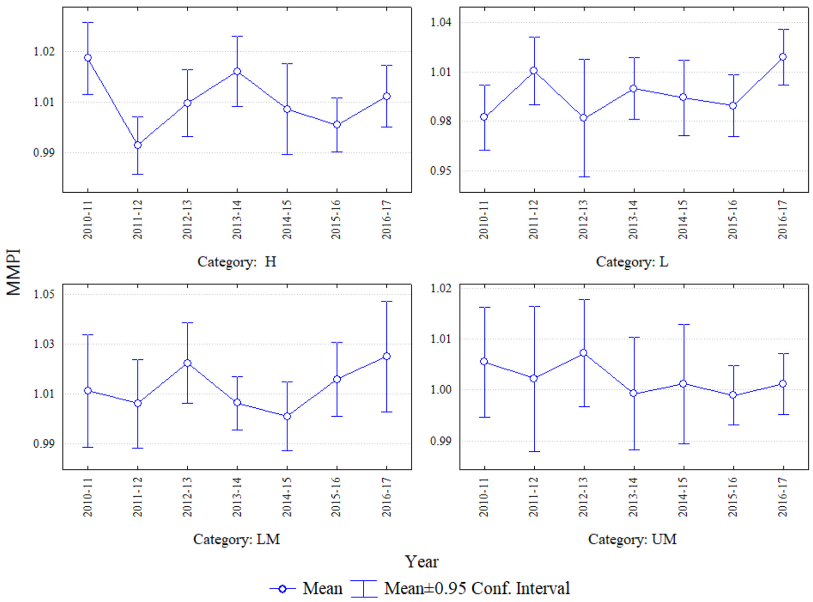
Figure 1 shows the average MMPI of four different income groups from 2010 to 2017. Unlike the three other income groups, most of the MMPIs are smaller than 1 for the low-income group. Only two periods, namely, 2010–2011 and 2016–2017, have MMPI values greater than 1. The average MMPI for the low-income group is 0.999, indicating a 0.1% regress annually in environmental efficiency. For the high-income group, the average annual MMPI is 1.007, and the values of MMPI are greater than 1 except for 2011–2012. The upper-middle and lower-middle-income groups also progressed during the research period. The average MMPI for the upper-middle group is 1.002. For the lower-middle-income group, the values of MMPI are greater than 1, except for 2014–2015. The annual improvement rate of the lower-middle-income group is 0.8%.
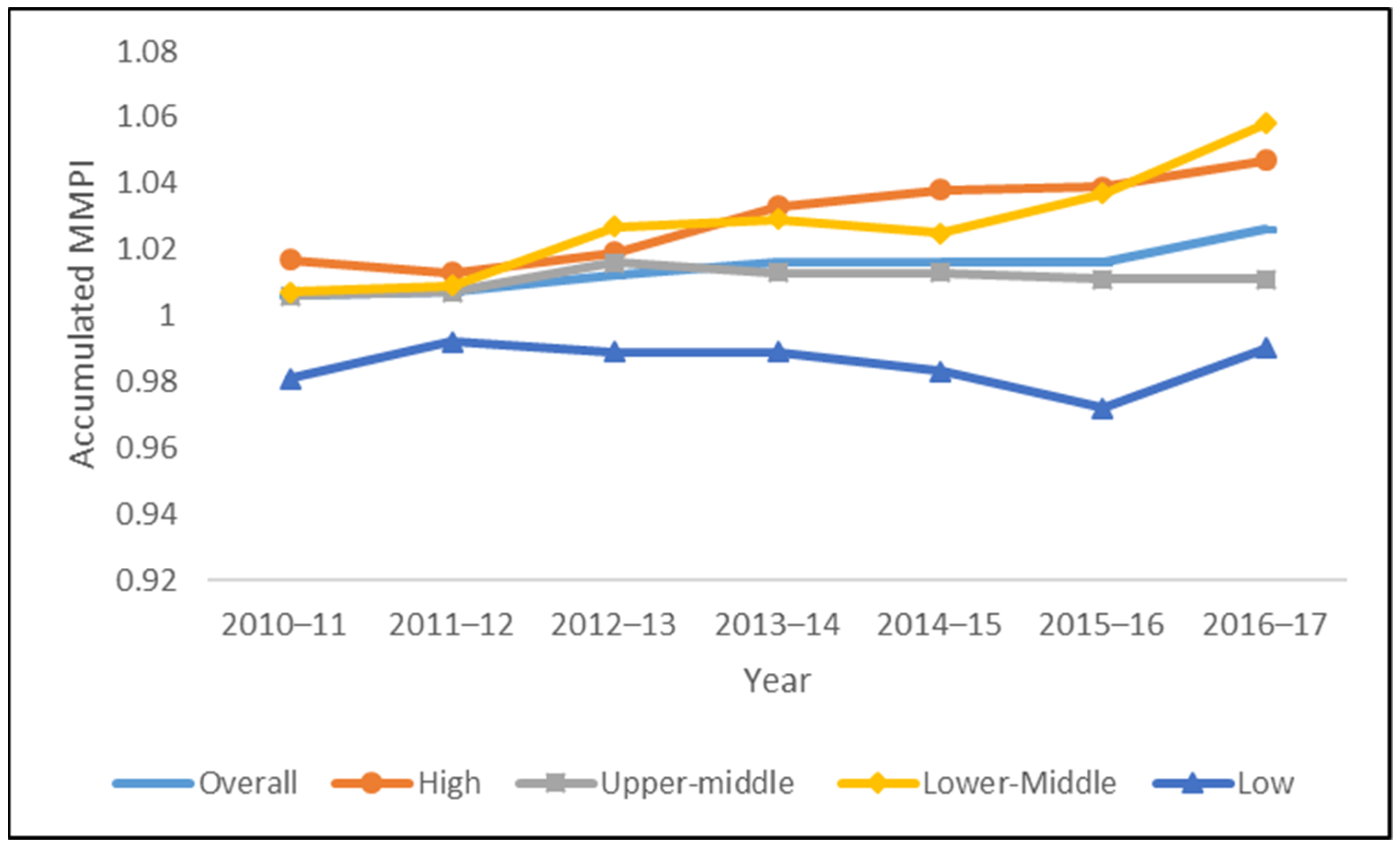
To investigate and compare the trend of MMPI among different groups further, the accumulated value of MMPI was calculated. Table 5 shows that the high-income group made the greatest progress because its accumulated value of MMPI is the largest. The low-income group suffered from regression in environmental efficiency. Figure 2 presents the trend of MMPI among different groups. The MMPI shows an upward trend for the high-income and lower-middle-income group. The trend for the upper-middle-income group is flatter, although the environmental efficiency is improving. Only the low-income group regressed, although the MMPI rose from 2016 to 2017. To understand the factors that influence the performance of different income groups, the next section decomposes the MMPI.

3.2. Decomposition of MMPI

The results of the Kruskal–Wallis test in Table 6 support differences among different income groups for MMPI. Further investigation will bring insights into the causes of improvement or degradation in environmental efficiency because MMPI can be decomposed into MMPI = EC*BPGC*TGRC.
The dynamic productivity change may stem from EC (catching-up) or BPGC (innovation). From the perspective of EC, only the high-income group shows a value lower than 1 (0.993). The values of EC for the upper-middle-income, lower-middle-income, and low-income groups are 1.010, 1.017, and 1.023, respectively. The room for maneuvering the input–output combination is very minimal for the high-income countries. By contrast, catching up is relatively easy for the three other groups [19].
For the high-income group, its BPGC is larger than 1, whereas its EC is less than 1. These results indicate that the improvement of environmental efficiency stems from frontier shifts rather than efficiency change, that is, the innovation effect contributes to the improvement of environmental efficiency, not the management capability, for high-income countries. These results echo the finding of [8,50] that the environmentally sensitive productivity growth of 26 OECD countries is mainly due to technical change. The lower-income countries (including lower-middle-income groups and low-income groups) have much less capability and capital to develop advanced, innovative environmental technology.
As to TGRC, among the four income groups, only the low-income group has a value less than 1, which means the low-income group lags behind the overall frontier. The upper-middle-income group (TGRC = 1.024) is moving toward the global frontier most rapidly, followed by the lower-middle-income group (TGRC = 1.003) and the high-income group (TGRC = 1.001). However, a higher TGRC does not guarantee the position of a global technology leader because TGRC is the change rate of the technology leadership [33]. More detailed information about TGR is needed to identify which group is the global technology leader in environmental efficiency.
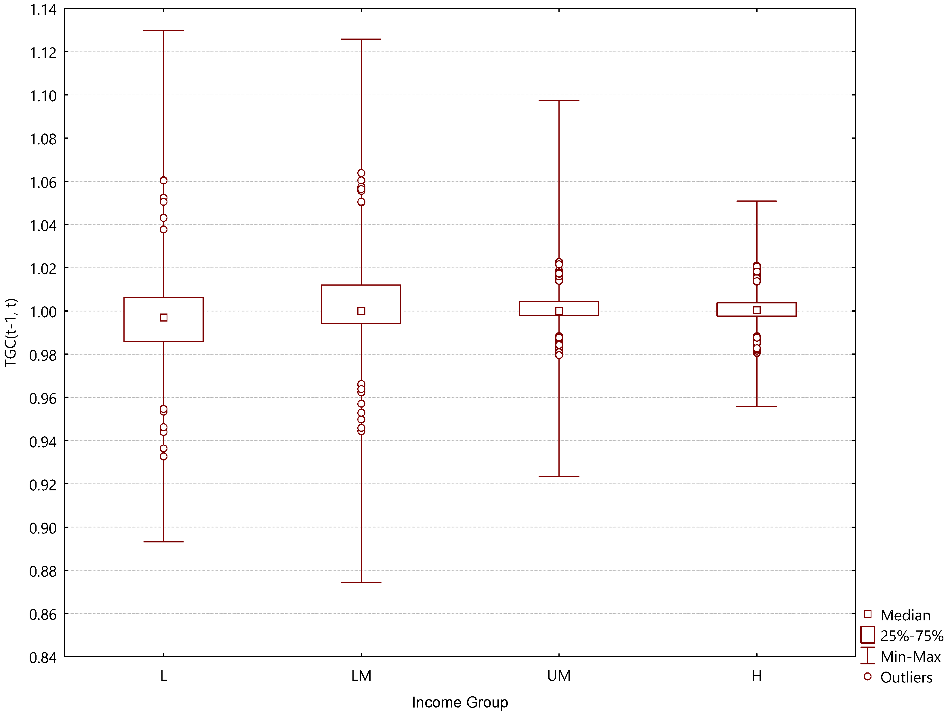
Figure 3 presents the boxplot of different income groups according to their median and variance. The lower-middle-income group has the largest variance among the four groups, whereas the high-income group has the least variance. Countries of low and lower-middle income have more extremes that either perform much better or worse than most other countries in their groups. Therefore, several of them are very far from the global frontier compared with their peers in the same group. By contrast, the high-income countries demonstrate homogeneity in terms of TGRC. In addition, the boxplot shows that more countries of the high- and upper-middle-income group are located at the global frontier.

3.3. Comparison of Environmental Efficiency before and after the Paris Agreement

Under the framework of the Kyoto Protocol, only the majority of the high-income group members have the responsibility to reduce GHG emissions, that is, compared with the three other groups (upper-middle-, lower-middle-, and low-income groups), the high-income group members have the incentive and pressure to increase their environmental efficiency. The empirical results also demonstrate that the high-income group makes progress in environmental efficiency.
The Paris Agreement has two distinctive features apart from the Kyoto Protocol. First, all signatories, not only industrialized countries, are obligated to contributions to mitigation. Second, all signatories determine their own contributions based on their own capabilities and conditions instead of being assigned by an international treaty. With the shift from the “top-down” to the “bottom-up” approach for the climate treaty, all countries, not only the industrialized countries, have to exert effort in mitigation since the adoption of the Paris Agreement. Therefore, any difference in environmental efficiency performance before and after the adoption of Paris Agreement must be determined for the three other income groups because they need to contribute to the mitigation after the adoption of the Paris Agreement. Table 7 shows that only the lower-middle-income group shows a statistical difference in terms of MMPI between the two periods. Its MMPI increases from an average value of 1.005 to 1.016.
However, the decomposition of MMPI reveals more insights. The BPGC of the high- income group deteriorates after the adoption of the Paris Agreement. In 2016, the newly elected US President Donald Trump posed potential threats to the implementation of the Paris Agreement because he has been skeptical about climate change and vowed to withdraw from the Paris Agreement during his campaign. Concerns were raised that other countries would follow the US lead in postponing their research and development of renewable energy [51,52]. The retreat of the US from the international climate governance may upset and cause the fluctuation of mitigation efforts for industrialized countries.
The EC of the upper-middle-income and lower-middle-income groups improved from the first period to the second period, indicating their enhanced capabilities to allocate resources. The picture of the low-income group is different. The value of EC for the low-income group worsened following the adoption of the Paris Agreement, whereas the value of BPGC increased, indicating a technology improvement for the low-income group.

4. Conclusions

Climate change is a major challenge to humankind, but eliminating poverty is also an arduous, important task for decision-makers or country leaders. Combating global warming and enhancing living standard simultaneously relies on environmental efficiency improvement. Thus, this study estimates the environmental efficiency of 150 economies during 2010–2017 to understand the worldwide trend. This research also intends to compare whether the environmental efficiency performance exhibited any difference before and after the implementation of the Paris Agreement.
This research adopts DEA and the Malmquist index to compare and capture the dynamic change of environmental efficiency among different income groups. Considering the heterogeneity of countries, a meta-frontier framework is also applied. The empirical results show that among the four income groups, only the low-income group suffered from regression in terms of environmental efficiency during the research period based on their average MMPI. The high-income group made the greatest progress because its accumulated value of MMPI is the largest. The improvement for the high-income group came from frontier shifts rather than efficiency change. By contrast, the improvement of the lower-income groups came from the catching-up effect. As to the impact of the Paris Agreement, only the lower-middle-income group showed a statistical difference between the two periods, and its environmental efficiency increased after the adoption of the Paris Agreement.
The results provide important policy implications. The statistical results support differences in terms of environmental efficiency among the four income groups, especially that the low-income group is in deterioration. Combatting global warming successfully cannot rely on specific countries. The world as a whole needs to cooperate and improve together, thus, more help needs to be devoted to the low-income group.
This study emphasizes the macro view about the differences among different groups, and the detailed discussion about specific countries is not the focus of this analysis. Moreover, the study period only covers two years after the Paris Agreement under the constraint of data availability, hence, a long-term trend cannot be observed. For future analysis, a longer-term comparison will provide more information about the effect of a bottom-up approach. An in-depth study to explore the benchmark country for each group will also be beneficial for poor performers to catch up.

Author Contributions

Conceptualization, W.-C.Y.; methodology, W.-M.L. and W.-C.Y.; software, W.-M.L.; validation, W.-C.Y. and W.-M.L.; formal analysis, W.-C.Y.; investigation, W.-C.Y.; resources, W.-C.Y. and W.-M.L.; data curation, W.-C.Y.; writing—original draft preparation, W.-C.Y.; writing—review and editing, W.-C.Y. and A.P.R.; visualization, W.-C.Y.; supervision, W.-C.Y.; project administration, W.-C.Y.; funding acquisition, W.-C.Y. and A.P.R. All authors have read and agreed to the published version of the manuscript.

Funding

This research received no external funding.

Institutional Review Board Statement

Not applicable.

Informed Consent Statement

Not applicable.

Data Availability Statement

All data will be available on reasonable request.

Acknowledgments

The authors thank three anonymous reviewers for their constructive comments. The first author is thankful for financial support from Taiwan’s Ministry of Science and Technology (MOST 108–2410–H–004–005).

Conflicts of Interest

The authors declare no conflict of interest.

References

  1. WEF. The Global Risks Report 2021; World Economic Forum: Cologny, Switzerland, 2021. [Google Scholar]
  2. IPCC. Special Report on Global Warming of 1.5 °C; The Intergovernmental Panel on Climate Change: Geneva, Switzerland, 2018. [Google Scholar]
  3. Falkner, R. The Paris Agreement and the new logic of international climate politics. Int. Aff. 2016, 92, 1107–1125. [Google Scholar] [CrossRef]
  4. UNFCCC. The Paris Agreement. Available online: https://unfccc.int/process-and-meetings/the-paris-agreement/the-paris-agreement (accessed on 16 February 2021).
  5. Zhang, N.; Wang, B.; Chen, Z. Carbon emissions reductions and technology gaps in the world’s factory, 1990–2012. Energy Policy 2016, 91, 28–37. [Google Scholar] [CrossRef]
  6. Feng, Y.; Liu, R.; Chiu, Y.-H.; Chang, T.-H. Dynamic Linkages Among Energy Consumption, Environment and Health Sustainability: Evidence from the Different Income Level Countries. Inq. J. Heal. Care Organ. Provis. Financ. 2020, 57, 1–18. [Google Scholar] [CrossRef]
  7. Kraft, J.; Kraft, A. On the Relationship between Energy and GNP. J. Energy Dev. 1978, 3, 401–403. [Google Scholar]
  8. Chiu, C.-R.; Liou, J.-L.; Wu, P.-I.; Fang, C.-L. Decomposition of the environmental inefficiency of the meta-frontier with undesirable output. Energy Econ. 2012, 34, 1392–1399. [Google Scholar] [CrossRef]
  9. Song, M.; An, Q.; Zhang, W.; Wang, Z.; Wu, J. Environmental efficiency evaluation based on data envelopment analysis: A review. Renew. Sustain. Energy Rev. 2012, 16, 4465–4469. [Google Scholar] [CrossRef]
  10. Ramanathan, R. Combining indicators of energy consumption and CO2 emissions: A cross-country comparison. Int. J. Glob. Energy Issues 2002, 17, 214–227. [Google Scholar] [CrossRef]
  11. Zhou, P.; Ang, B.; Poh, K. A survey of data envelopment analysis in energy and environmental studies. Eur. J. Oper. Res. 2008, 189, 1–18. [Google Scholar] [CrossRef]
  12. Castro, P. Past and future of burden sharing in the climate regime: Positions and ambition from a top-down to a bottom-up governance system. Int. Environ. Agreem. Politics Law Econ. 2020, 20, 41–60. [Google Scholar] [CrossRef]
  13. Arcelus, F.J.; Arocena, P. Productivity differences across OECD countries in the presence of environmental constraints. J. Oper. Res. Soc. 2005, 56, 1352–1362. [Google Scholar] [CrossRef]
  14. Färe, R.; Grosskopf, S.; Hernandez-Sancho, F. Environmental performance: An index number approach. Resour. Energy Econ. 2004, 26, 343–352. [Google Scholar] [CrossRef]
  15. Zaim, O.; Taskin, F. A Kuznets Curve in Environmental Efficiency: An Application on OECD Countries. Environ. Resour. Econ. 2000, 17, 21–36. [Google Scholar] [CrossRef]
  16. Rashidi, K.; Shabani, A.; Saen, R.F. Using data envelopment analysis for estimating energy saving and undesirable output abatement: A case study in the Organization for Economic Co-Operation and Development (OECD) countries. J. Clean. Prod. 2015, 105, 241–252. [Google Scholar] [CrossRef]
  17. Iram, R.; Zhang, J.; Erdogan, S.; Abbas, Q.; Mohsin, M. Economics of energy and environmental efficiency: Evidence from OECD countries. Environ. Sci. Pollut. Res. 2020, 27, 3858–3870. [Google Scholar] [CrossRef] [PubMed]
  18. Kumar, S.; Khanna, M. Measurement of environmental efficiency and productivity: A cross-country analysis. Environ. Dev. Econ. 2009, 14, 473–495. [Google Scholar] [CrossRef] [Green Version]
  19. Lin, E.Y.-Y.; Chen, P.-Y.; Chen, C.-C. Measuring green productivity of country: A generalized metafrontier Malmquist productivity index approach. Energy 2013, 55, 340–353. [Google Scholar] [CrossRef]
  20. Parks, B.C.; Roberts, J.T. Inequality and the global climate regime: Breaking the north-south impasse. Camb. Rev. Int. Aff. 2008, 21, 621–648. [Google Scholar] [CrossRef]
  21. Li, M.; Wang, Q. International environmental efficiency differences and their determinants. Energy 2014, 78, 411–420. [Google Scholar] [CrossRef]
  22. Li, K.; Lin, B. Metafroniter energy efficiency with CO2 emissions and its convergence analysis for China. Energy Econ. 2015, 48, 230–241. [Google Scholar] [CrossRef]
  23. Lin, E.Y.-Y.; Chen, P.-Y.; Chen, C.-C. Measuring the environmental efficiency of countries: A directional distance function metafrontier approach. J. Environ. Manag. 2013, 119, 134–142. [Google Scholar] [CrossRef]
  24. Zhou, P.; Ang, B.; Han, J. Total factor carbon emission performance: A Malmquist index analysis. Energy Econ. 2010, 32, 194–201. [Google Scholar] [CrossRef]
  25. Chang, M.-C. Applying the energy productivity index that considers maximized energy reduction on SADC (Southern Africa Development Community) members. Energy 2016, 95, 313–323. [Google Scholar] [CrossRef]
  26. Chang, M.-C.; Hu, J.-L.; Chang, H.-C. Resource Efficiency and Productivity Changes in the G7 and BRICS Nations. Pol. J. Environ. Stud. 2018, 27, 2463–2474. [Google Scholar] [CrossRef]
  27. EIA. International Energy Data. Available online: https://www.eia.gov/international/overview/world (accessed on 15 August 2020).
  28. Feenstra, R.C.; Inklaar, R.; Timmer, M.P. The Next Generation of the Penn World Table. Am. Econ. Rev. 2015, 105, 3150–3182. [Google Scholar] [CrossRef] [Green Version]
  29. Seiford, L.M.; Zhu, J. Modeling undesirable factors in efficiency evaluation. Eur. J. Oper. Res. 2002, 142, 16–20. [Google Scholar] [CrossRef]
  30. Chung, Y.H.; Färe, R.; Grosskopf, S. Productivity and Undesirable Outputs: A Directional Distance Function Approach. J. Environ. Manag. 1997, 51, 229–240. [Google Scholar] [CrossRef] [Green Version]
  31. Cooper, W.W.; Seiford, L.M.; Tone, K. Data Envelopment Analysis: A Comprehensive Text with Models, Applications, Reference and DEA-Solver Software, 2nd ed.; Springer Science Business Media: New York, NY, USA, 2007. [Google Scholar]
  32. O’Donnell, C.J.; Rao, D.S.P.; Battese, G.E. Metafrontier frameworks for the study of firm-level efficiencies and technology ratios. Empir. Econ. 2008, 34, 231–255. [Google Scholar] [CrossRef]
  33. Oh, D.-H.; Lee, J.-D. A metafrontier approach for measuring Malmquist productivity index. Empir. Econ. 2010, 38, 47–64. [Google Scholar] [CrossRef]
  34. Battese, G.E.; Rao, D.P. Technology Gap, Efficiency, and a Stochastic Metafrontier Function. Int. J. Bus. Econ. 2002, 1, 87–93. [Google Scholar]
  35. World Bank. How Are the Income Group Thresholds Determined. Available online: https://datahelpdesk.worldbank.org/knowledgebase/articles/378833-how-are-the-income-group-thresholds-determined (accessed on 3 September 2020).
  36. Farnum, N.R. Using Johnson curves to describe non-normal process data. Qual. Eng. 1996, 9, 329–336. [Google Scholar] [CrossRef]
  37. Brockett, P.L.; Golany, B. Using Rank Statistics for Determining Programmatic Efficiency Differences in Data Envelopment Analysis. Manag. Sci. 1996, 42, 466–472. [Google Scholar] [CrossRef]
  38. Malmquist, S. Index numbers and indifference surfaces. Trab. Estad. 1953, 4, 209–242. [Google Scholar] [CrossRef]
  39. Färe, R.; Grosskopf, S.; Lovell, C.A.K.; Grifell-Tatjé, E. Biased Technical Change and the Malmquist Productivity Index. Scand. J. Econ. 1997, 99, 119–127. [Google Scholar] [CrossRef]
  40. Caves, D.W.; Christensen, L.R.; Diewert, W.E. The Economic Theory of Index Numbers and the Measurement of Input, Output, and Productivity. Econometrica 1982, 50, 1393. [Google Scholar] [CrossRef]
  41. Färe, R.; Grosskopf, S.; Lindgren, B.; Roos, P. Productivity Developments in Swedish Hospitals: A Malmquist Output Index Approach. In Data Envelopment Analysis: Theory, Methodology and Applications; Charnes, A., Cooper, W.W., Lewin, A.Y., Seiford, L.M., Eds.; Kluwer Academic Publishers: Boston, MA, USA, 1994; pp. 254–272. [Google Scholar] [CrossRef]
  42. Orea, L. Parametric Decomposition of a Generalized Malmquist Productivity Index. J. Prod. Anal. 2002, 18, 5–22. [Google Scholar] [CrossRef]
  43. Färe, R.; Grosskopf, S.; Norris, M.; Zhang, Z. Productivity Growth, Technical Progress, and Efficiency Change in Industrialized Countries. Am. Econ. Rev. 1994, 84, 66–83. [Google Scholar]
  44. Portela, M.; Thanassoulis, E.; Horncastle, A.; Maugg, T. Productivity change in the water industry in England and Wales: Application of the meta-Malmquist index. J. Oper. Res. Soc. 2011, 62, 2173–2188. [Google Scholar] [CrossRef]
  45. Wu, J.; Zhu, Q.; Yin, P.; Song, M. Measuring energy and environmental performance for regions in China by using DEA-based Malmquist indices. Oper. Res. 2015, 17, 715–735. [Google Scholar] [CrossRef]
  46. Lin, B.; Chen, X. Evaluating the CO2 performance of China’s non-ferrous metals Industry: A total factor meta-frontier Malmquist index perspective. J. Clean. Prod. 2019, 209, 1061–1077. [Google Scholar] [CrossRef]
  47. Munisamy, S.; Arabi, B. Eco-efficiency change in power plants: Using a slacks-based measure for the meta-frontier Malmquist–Luenberger productivity index. J. Clean. Prod. 2015, 105, 218–232. [Google Scholar] [CrossRef]
  48. Hayami, Y.; Ruttan, V.W. Agricultural Productivity Differences among Countries. Am. Econ. Rev. 1970, 60, 895–911. [Google Scholar]
  49. Pastor, J.T.; Lovell, C.A.K. A global Malmquist productivity index. Econ. Lett. 2005, 88, 266–271. [Google Scholar] [CrossRef]
  50. Oh, D.-H. A global Malmquist-Luenberger productivity index. J. Prod. Anal. 2010, 34, 183–197. [Google Scholar] [CrossRef]
  51. Zhang, H.-B.; Dai, H.-C.; Lai, H.-X.; Wang, W.-T. U.S. withdrawal from the Paris Agreement: Reasons, impacts, and China’s response. Adv. Clim. Chang. Res. 2017, 8, 220–225. [Google Scholar] [CrossRef]
  52. Sanderson, B.M.; Knutti, R. Delays in US mitigation could rule out Paris targets. Nat. Clim. Chang. 2017, 7, 92–94. [Google Scholar] [CrossRef]
Figure 1. Mean Plot of MMPI of Different Income Groups. Note: This figure depicts the average meta-frontier Malmquist performance index for four different income groups: the high-income group (denoted as H), the upper-middle-income group (denoted as UM), the lower-middle-income group (denoted as LM), and the low-income group (denoted as L).
Energies 14 04503 g001
Figure 2. Accumulated MMPI of Different Income Groups. Note: This figure presents the trend of environmental efficiency of different income groups from 2010 to 2017 based on their estimated accumulated meta-frontier Malmquist performance index.
Energies 14 04503 g002
Figure 3. Boxplot of TGRC of different income groups. Note: This figure demonstrates the boxplot of different income groups based on their average technology gap ratio change from 2010 to 2017. This figure also shows the median and variance of each income group for comparison.
Energies 14 04503 g003
Table 1. Input and Output Variables to Estimate Environmental Efficiency.
VariableDefinitionUnitSource
x1Labor forceMillion peoplePenn World Table
Inputx2Energy consumptionPJUS EIA
x3Capital stockBillion 2017 US dollarsPenn World Table
Desirable Outputy1GDPBillion 2017 US dollarsPenn World Table
Undesirable outputy2CO2 emissionsMillion metric tonesUS EIA
Table 2. Data Set of 150 Economies.
GroupAnnex IList of Countries in the Group
High-incomeYesAustralia, Austria, Belgium, Canada, Croatia, Cyprus, Czech Republic, Denmark, Estonia, Finland, France, Germany, Greece, Hungary, Iceland, Ireland, Italy, Japan, Latvia, Lithuania, Luxembourg, Malta, Netherlands, New Zealand, Norway, Poland, Portugal, Slovakia, Slovenia, Spain, Sweden, Switzerland, United Kingdom, United States
NoArgentina, Aruba, Bahrain, Barbados, Chile, Israel, Kuwait, Oman, Panama, Qatar, Saudi Arabia, Seychelles, Singapore, Taiwan, Trinidad and Tobago, United Arab Emirates, Uruguay
Upper-middle incomeYesBelarus, Bulgaria, Romania, Turkey
NoAlbania, Algeria, Armenia, Azerbaijan, Belize, Bosnia and Herzegovina, Botswana, Brazil, China, Colombia, Costa Rica, Dominican Republic, Ecuador, Equatorial Guinea, Fiji, Gabon, Grenada, Guatemala, Iraq, Jamaica, Jordan, Kazakhstan, Lebanon, Malaysia, Maldives, Mauritius, Mexico, Montenegro, Namibia, North Macedonia, Paraguay, Peru, Saint Lucia, Serbia, South Africa, Suriname, Thailand
Lower-middle incomeNoAngola, Bangladesh, Bhutan, Cabo Verde, Cambodia, Cameroon, Djibouti, Egypt, El Salvador, Eswatini, Georgia, Ghana, Honduras, India, Indonesia, Kenya, Kyrgyzstan, Lesotho, Mauritania, Mongolia, Morocco, Nicaragua, Nigeria, Pakistan, Philippines, Sri Lanka, Sudan, Tunisia, Ukraine, Uzbekistan, Zambia
Low-incomeNoBenin, Burkina Faso, Burundi, Central African Republic, Chad, Comoros, Ethiopia, Guinea, Guinea-Bissau, Haiti, Liberia, Madagascar, Malawi, Mali, Mozambique, Nepal, Niger, Rwanda, Sao Tome and Principe, Senegal, Sierra Leone, Tajikistan, Togo, Uganda, Yemen, Zimbabwe
Annex I countries are categorized by the UNFCCC which are obliged for higher commitment for mitigation.
Table 3. Descriptive statistics for all input and output factors by different income groups.
GroupVariableMeanMedianMinMaxS. D.VarianceTest of Normality
Hx110.5843.3910.043154.44022.862523.000<0.01 ***
x25.1061.2840.013103.68114.480209.658<0.01 ***
x33757.1191194.54911.92456,215.3108323.28569,277,075.000<0.01 ***
y1938.487267.5431.81017,711.0202394.2245,732,311.000<0.01 ***
y2267.16256.5570.9085585.600757.408573,667.000<0.01 ***
UMx127.6592.8840.053792.580120.02014,406.000<0.01 ***
x24.7670.3620.004147.10421.048443.038<0.01 ***
x32802.006282.3054.61694,903.73011,005.070121,111,472.000<0.01 ***
y1702.69987.5071.08618,978.5002507.3206,286,667.000<0.01 ***
y2327.82721.0410.27110,801.7701560.6102,435,496.000<0.01 ***
LMx132.5007.6060.175537.83090.9588273.000<0.01 ***
x21.8490.2600.01032.1535.04925.493<0.01 ***
x31764.667310.1447.29329,931.0704761.90522,675,741.000<0.01 ***
y1506.796112.1471.9358769.1801301.8381,694,782.000<0.01 ***
y2118.97914.1790.4002312.060359.703129,386.000<0.01 ***
Lx16.8014.5370.04847.9198.32769.345<0.01 ***
x20.0760.0420.0020.3690.0870.008<0.01 ***
x387.94450.0303.286625.93396.3199277.300<0.01 ***
y129.43021.4550.588188.20631.481991.077<0.01 ***
y23.6512.4830.10024.3404.25518.106<0.01 ***
H: the high-income group; UM: the upper-middle-income group; LM: the lower-middle-income group; L: the low-income group. x1: labor force; x2: energy consumption; x3: capital stock; y1: GDP; y2: CO2 emissions. The asterisks *** indicate significance levels of 1%.
Table 4. Kruskal–Wallis test of all variables in four income groups.
LaborEnergyCapitalGDPCO2
Kruskal–Wallis test37.155363.766312.975253.743353.961
p-value0.000 ***0.000 ***0.000 ***0.000 ***0.000 ***
1 The asterisks *** indicate significance levels of 10%, 5%, and 1% or better, respectively.
Table 5. Average and Accumulated MMPI of Different Income Groups.
GroupOverallHighUpper MiddleLower MiddleLow
YearAve. MMPIAccu. MMPIAve. MMPIAccu. MMPIAve. MMPIAccu. MMPIAve. MMPIAccu. MMPIAve. MMPIAccu. MMPI
2010–20111.0061.0061.0171.0171.0061.0061.0071.0070.9810.981
2011–20121.0011.0070.9961.0131.0011.0071.0021.0091.0100.992
2012–20131.0051.0121.0061.0191.0081.0161.0181.0270.9980.989
2013–20141.0041.0161.0141.0330.9981.0131.0021.0290.9990.989
2014–20151.0001.0161.0051.0381.0001.0130.9971.0250.9940.983
2015–20161.0001.0161.0011.0390.9971.0111.0111.0370.9890.972
2016–20171.0101.0261.0081.0471.0001.0111.0211.0581.0190.990
Ave.1.0041.0141.0071.0301.0021.0111.0081.0270.9990.985
Ave. MMPI is the average MMPI value; Accu. MMPI is the accumulated MMPI value. Accumulated MMPI is calculated as follows: deduct the numerical value 1 (value 1 represents neutrality in efficiency) from the average MMPI and add the resulting value to the previous year’s accumulated MMPI value.
Table 6. Difference test of environmental efficiency among different income groups.
2010–2017Income LevelAverageStandard DeviationKruskal–Wallis Test (p-Value)
MMPIHigh1.0070.0310.017 **
Upper-Middle1.0020.044
Lower-Middle1.0080.048
Low0.9960.058
ECHigh0.9930.0470.000 ***
Upper-Middle1.0100.064
Lower-Middle1.0170.057
Low1.0230.073
BPGCHigh1.0140.0480.000 ***
Upper-Middle1.0170.057
Lower-Middle0.9900.043
Low0.9810.057
The asterisks **, and *** indicate significance levels of 10%, 5%, and 1% or better, respectively.
Table 7. Comparison of Environmental Efficiency Pre- and Post-Paris Agreement.
GroupEfficiency2010–20152015–2017Kruskal-Wallis Test (p-Value)
HighMMPI1.0081.0040.484
EC0.9891.0030.051
BPGC1.0191.001 0.004 ***
TGRC1.0011.0010.505
Upper-MiddleMMPI1.0030.9990.583
EC1.0071.017 0.036 **
BPGC0.9960.982 0.004 ***
TGRC1.0011.0010.435
Lower-MiddleMMPI1.0051.016 0.043 **
EC1.0151.023 0.012 **
BPGC0.9900.9890.243
TGRC1.0021.0040.983
LowMMPI0.9931.0040.159
EC1.0311.005 0.024 **
BPGC0.9721.004 0.001 ***
TGRC0.9940.9960.550
The asterisks **, and *** indicate significance levels of 10%, 5%, and 1% or better, respectively.
Publisher’s Note: MDPI stays neutral with regard to jurisdictional claims in published maps and institutional affiliations.